TAD-YOLO11n: A Lightweight Network with Multiscale Feature Enhancement for Steel Surface Defect Inspection

Abstract

Reliable and fast detection of steel surface defects is essential for quality control in intelligent manufacturing. In practical inspection scenarios, lightweight detectors still face challenges associated with low-contrast defect textures, the loss of fine edge information during downsampling, and insufficient interaction among features at different scales. To improve detection accuracy and computational efficiency, this study proposes TAD-YOLO11n, a lightweight multiscale feature-enhancement detector based on YOLO11n. In the backbone, C3k2-TFE-EMA is introduced to enhance the representation of weak textures and elongated defects by combining local texture enhancement, frequency-domain modeling, and EMA attention. ED-ADown is employed during downsampling to preserve edge details while reducing the parameter count and computational cost. In the neck, DynamicScalSeq+ASF is incorporated to promote adaptive interaction among P3, P4, and P5 features. Experiments on the NEU-DET dataset showed that TAD-YOLO11n achieved an mAP50 of 79.0%, exceeding the YOLO11n baseline by 4.8 percentage points. Meanwhile, the number of parameters decreased from 2.583 M to 2.106 M, and the computational cost decreased from 6.3 to 5.3 GFLOPs, while the inference speed reached 175.5 FPS. These results demonstrate that the proposed model improves detection performance under lightweight constraints and provides a practical solution for real-time steel surface defect inspection.

1. Introduction

Steel is widely used in equipment manufacturing, transportation, energy systems, and civil construction [1,2]. During rolling, cooling, handling, and storage, surface quality can be affected by equipment wear, temperature fluctuations, inclusions in the material, and external impacts. These factors may lead to surface defects such as crazing, inclusions, patches, pitted surfaces, rolled-in scale, and scratches. Such defects can degrade the mechanical properties, corrosion resistance, and service reliability of steel products. Therefore, accurate and efficient surface inspection is essential for product quality control and production safety.

Conventional steel surface inspection mainly relies on manual visual inspection or machine-vision methods based on handcrafted features. Manual inspection is inefficient and susceptible to variations in operator experience and fatigue. Handcrafted-feature-based methods generally rely on texture, edge, and grayscale descriptors, but their robustness decreases when defect appearances are complex, scale variations are large, or contrast is low. In recent years, deep learning has become a major approach to industrial defect inspection. Nevertheless, small defects, scale variation, background interference, and the trade-off between detection accuracy and inference speed remain major challenges. Therefore, lightweight network design and multiscale feature fusion are important for practical deployment [3,4].

Driven by the development of deep convolutional networks, object detection algorithms have been widely applied to industrial surface inspection. Current detectors can generally be divided into two-stage and one-stage frameworks. Two-stage detectors, represented by Faster R-CNN, usually provide high localization accuracy, but their multi-step inference process leads to a higher computational cost. One-stage detectors, including the YOLO series, perform classification and localization in a single forward pass and thus offer simpler architectures and faster inference. These characteristics make YOLO-type detectors more suitable for online steel surface defect inspection [5,6,7,8,9,10,11].

Recent studies have attempted to improve steel surface defect detection by introducing attention mechanisms, lightweight networks, and multiscale fusion strategies [12,13,14]. However, steel defects often exhibit low contrast, indistinct textures, small spatial extent, and substantial variations in shape. For example, crazing and rolled-in scale can be easily confused with rolling textures because of their low contrast and indistinct appearance, making it difficult to distinguish defect regions from the background. Scratches and pitted surfaces often occupy small regions and have blurred boundaries, making their features vulnerable to loss during feature-map downsampling. In addition, defect categories differ considerably in size and morphology, which limits the ability of fixed-path feature fusion to select useful scale information. Under lightweight constraints, simultaneously enhancing weak-texture representation, preserving fine details, and improving cross-scale feature interaction remains challenging.

To address the above challenges, this study develops TAD-YOLO11n, a lightweight multiscale feature enhancement network for steel surface defect inspection based on YOLO11n. The network follows a progressive feature-processing strategy. C3k2-TFE-EMA is embedded in the backbone to enhance weak-texture responses, ED-ADown is applied during resolution reduction to preserve edge and fine-structure information, and DynamicScalSeq+ASF is introduced into the neck to strengthen cross-scale feature interaction. This stage-wise arrangement improves the representation of low-contrast, elongated, and multiscale defects while maintaining a compact model structure. The methodological contribution lies in organizing these mechanisms according to the feature degradation process of steel surface defects, allowing weak-texture enhancement, detail preservation, and cross-scale interaction to be addressed sequentially within a compact detector.

The main contributions of this study are summarized as follows:

(1)

A C3k2-TFE-EMA weak-texture enhancement module is designed. It integrates local texture modeling, frequency-domain difference extraction, and EMA attention to improve the representation of low-contrast and slender defects.

(2)

An ED-ADown edge-detail-aware downsampling module is introduced. By combining convolutional learning with pooling-based saliency retention, this module reduces model complexity and alleviates the loss of small-defect details.

(3)

A DynamicScalSeq+ASF dynamic multiscale attention fusion structure is proposed. It aligns, aggregates, and filters P3, P4, and P5 features to strengthen information exchange across defect scales.

(4)

Ablation studies, comparative experiments, repeated trials, robustness evaluations, and cross-dataset experiments are conducted on the NEU-DET, GC10-DET, and Severstal Steel Defect datasets. The proposed method is evaluated in terms of detection accuracy, model complexity, training stability, robustness to image degradation, and cross-dataset adaptability.

2. Related Work

2.1. Research on Enhancing Features of Defects with Weak Textures and Complex Shapes

In steel surface defect inspection, defective regions often exhibit weak textures, low gray-level contrast, indistinct boundaries, and irregular shapes. Unlike common objects in natural images, these defects usually do not contain rich semantic cues. As a result, the detector must extract more information from local texture, boundary details, and grayscale differences. Improving the feature representation of weak-textured and irregularly shaped defects has therefore become an important research topic in this field.

Many early YOLO-based studies improved defect inspection mainly by strengthening feature extraction. Zhao et al. [15] developed RDD-YOLO by adding a Res2Net module and a dual-feature pyramid network, which improved multiscale defect representation. Lu et al. [16] proposed WSS-YOLO, where dynamic serpentine convolution was adopted to better capture elongated and irregular defects, and Slim-Neck was used to reduce the computational burden. These methods are useful for scale variation and shape irregularity. However, most feature enhancement is still performed in the spatial domain, which may be insufficient for distinguishing subtle texture differences between low-contrast defects and the steel background.

2.2. Research on Lightweight Detection and Detail Preservation

For industrial applications, steel defect detectors should maintain satisfactory detection accuracy while using fewer parameters and lower computational cost. Existing studies on lightweight detection generally improve deployment efficiency by reducing structural redundancy, adopting efficient convolutions, compressing networks, or simplifying feature fusion.

To obtain a trade-off between accuracy and complexity, Xie et al. [17] proposed a YOLOv8-based lightweight multiscale feature fusion model that improves feature expression through efficient convolution and attention. Liu et al. [18] further reduced redundant features by introducing lightweight structures such as ScConv and GSConv, thereby lowering computational load. Lu et al. [19] optimized the YOLOv7 architecture to improve detection performance with reduced model complexity. These studies demonstrate that lightweight components can effectively reduce the parameter count and computational cost, facilitating the industrial deployment of steel surface defect detection models.

Lightweight design involves more than simply compressing a model; it should also prevent critical defect details from being weakened during downsampling. Crazing, scratches, and pitted surfaces often occupy small regions and exhibit weak boundaries and fine textures. Repeated strided convolutions or pooling operations reduce feature-map resolution and may suppress these subtle cues. However, existing lightweight methods often place insufficient emphasis on detail preservation during downsampling. Therefore, an effective lightweight module should reduce computational redundancy while retaining local salient responses and sufficient feature representation capability, thereby avoiding excessive information loss for small and weak defects.

2.3. Research on Multiscale Feature Fusion and Cross-Scale Interaction

Steel surface defects differ markedly in size, shape, and texture distribution. Features from shallow layers contain richer edge and texture information and are helpful for locating fine defects, whereas deep features provide stronger semantic cues and are more suitable for recognizing large-area defects. Thus, multiscale feature fusion is an essential strategy for improving steel surface defect detection.

To cope with scale variation and background interference, Gao et al. [20] combined an attention mechanism with weighted BiFPN in YOLOv5 to improve cross-scale information propagation. Zhang et al. [21] integrated multiscale fusion with an attention residual module to improve classification and localization of hot-rolled steel defects. Yu et al. [22] proposed CRGF-YOLO by optimizing the feature fusion path of YOLOv5 and improving information exchange among defect features at different scales. Ni et al. [23] introduced lightweight feature extraction, multiscale fusion, and receptive-field attention into YOLOv8n for small-defect detection. Li et al. [24] built a multilayer fusion network by combining RepBi-PAN, DenseNet, and NAM attention in YOLOv5 to enhance defect recognition in complex backgrounds.

Although previous studies have advanced weak-texture representation, lightweight design, and multiscale feature fusion, most address these issues separately. Steel surface defect detection, however, requires them to be considered jointly because low-contrast textures, fine structures, and large-scale variations often occur simultaneously. To address this limitation, TAD-YOLO11n introduces a three-stage design that integrates texture enhancement, detail-preserving downsampling, and multiscale feature fusion within a compact YOLO11n framework. By addressing these aspects at different stages of the detector, TAD-YOLO11n provides a more balanced lightweight solution for steel surface defect detection than methods centered on a single structural modification.

3. TAD-YOLO11n Algorithm

3.1. Optimization of YOLO11n

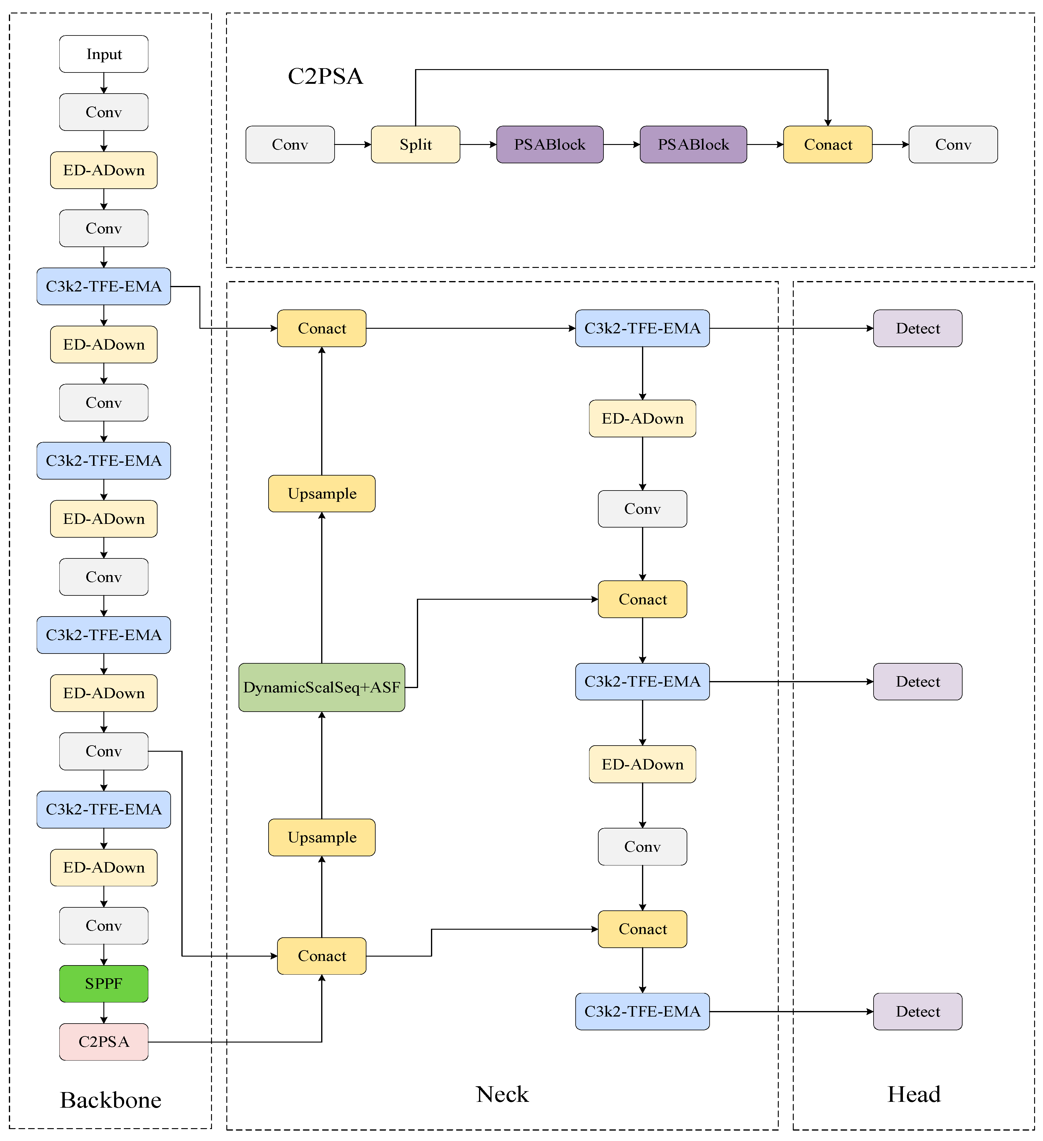
Based on YOLO11n, the proposed TAD-YOLO11n model introduces targeted improvements in the backbone, downsampling path, and neck. First, C3k2-TFE-EMA is inserted into the backbone to improve the extraction of low-contrast textures through local texture enhancement, frequency-domain difference modeling, and EMA attention. Second, ED-ADown replaces part of the original convolutional downsampling structure to reduce the loss of small-object and weak-edge information. Its convolution branch maintains learnable feature extraction, while its pooling branch retains local saliency responses. Third, DynamicScalSeq+ASF is placed in the neck to align, dynamically aggregate, and filter P3, P4, and P5 features. This arrangement enables the weak-texture responses enhanced in the backbone to be retained during downsampling and subsequently integrated across multiple scales in the neck, forming a continuous feature-enhancement process throughout the detector. The overall architecture of TAD-YOLO11n is shown in Figure 1.

Figure 1 shows that TAD-YOLO11n is composed of a backbone, neck, and head. In the backbone, C3k2-TFE-EMA and ED-ADown are alternately introduced to improve weak-texture feature extraction, reduce detail loss, and decrease computation. SPPF and C2PSA are retained at the end of the backbone to strengthen high-level semantic representation. In the neck, multiscale information is refined by upsampling, concatenation, and C3k2-TFE-EMA, and the DynamicScalSeq+ASF module is used to fuse P3, P4, and P5 features adaptively. The head uses the detect layer for multiscale classification and localization. This architecture aims to improve detection accuracy while keeping the network lightweight.

3.2. C3k2-TFE-EMA

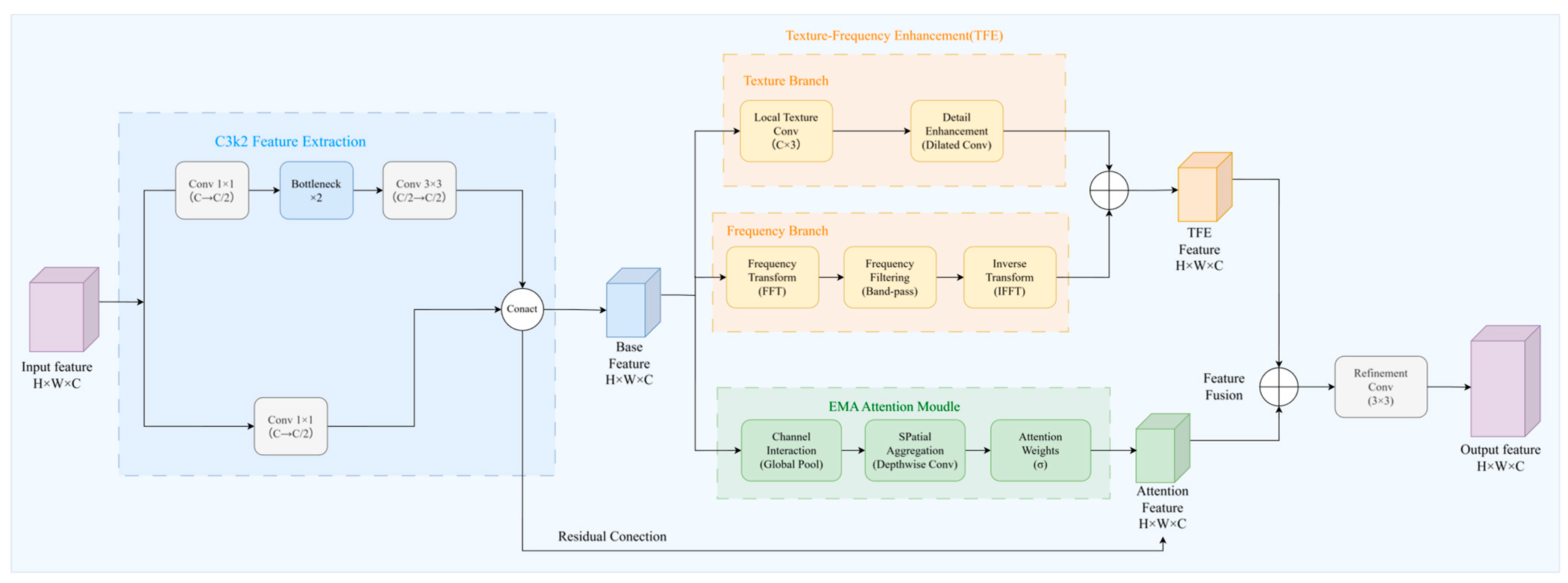
To improve the representation of low-contrast textures, slender defects, and complex backgrounds, C3k2-TFE-EMA is developed by integrating texture enhancement, frequency-domain filtering, and EMA attention into C3k2 [25]. After C3k2 extracts the base feature $F_{\mathrm{c}}$, the texture branch strengthens local gradients, edges, and fine structures, which benefits the detection of elongated defects such as crazing and scratches. The frequency-domain branch transforms $F_{\mathrm{c}}$ into the spectral domain. Low-frequency components mainly describe slowly varying illumination and global surface structures, whereas relatively high-frequency components contain local intensity transitions, edges, and fine textures. Steel surface defects often appear as weak and sparse disturbances superimposed on repetitive background textures. Their spectral responses can therefore provide complementary information that may be weakened by repeated spatial convolution and downsampling. The frequency-domain filtering weights selectively adjust different spectral components before inverse transformation. The EMA branch further recalibrates channel and spatial responses to suppress irrelevant background activations and emphasize defect-related regions. Finally, the enhanced features from the three branches are fused using learnable weights and combined with the input through a residual connection. The computation is formulated as follows:

$$F_{\mathrm{t}}=\delta \left(W_{\mathrm{t}}\times F_{\mathrm{c}}+b_{\mathrm{t}}\right)$$

(1)

$$F_{\mathrm{f}}=F^{-1}\left(M\odot F\left(F_{\mathrm{c}}\right)\right)$$

(2)

$$Y=X+W_{\mathrm{o}}\times \left(\alpha F_{\mathrm{t}}+\beta F_{\mathrm{f}}+\gamma F_{\mathrm{a}}\right)+b_{\mathrm{o}}$$

(3)

In the equation, $X$ is the input feature map; $F_c$ represents the base features extracted by C3k2; $F_{\mathrm{t}}$, $F_{\mathrm{f}}$, and $F_{\mathrm{a}}$ represent the texture-enhanced, frequency-domain-enhanced, and EMA-enhanced features, respectively; and $F\left(·\right)$ and $F^{-1}\left(·\right)$ denote the Fourier transform and inverse Fourier transform. $M$ denotes a learnable frequency-domain weighting matrix that is jointly optimized with the other network parameters through backpropagation. No static or manually defined frequency threshold is used. During training, $M$ adaptively reweights different spectral components, and the weighted spectrum is transformed back into the spatial domain to obtain $F_{\mathrm{f}}$. The operator $\odot$ denotes element-wise multiplication. In addition, $\delta \left(·\right)$ represents the nonlinear activation function; $W_{\mathrm{t}}$ and $W_{\mathrm{o}}$ represent learnable weights; $b_{\mathrm{t}}$ and $b_{\mathrm{o}}$ are bias terms; $\alpha$, $\beta$, and $\gamma$ represent the fusion weights for different branches; and $Y$ represents the module’s output features. The structural diagram of the C3k2-TFE-EMA module is shown in Figure 2.

Figure 2 presents the internal feature flow of C3k2-TFE-EMA. The input is first processed by the C3k2 unit to obtain the base feature $F_{\mathrm{c}}$, which is then delivered to the TFE and EMA branches. In TFE, the texture and frequency-domain branches operate in parallel to extract local structural details and spectral information. EMA generates channel–spatial attention responses from the base feature. The TFE-enhanced features, EMA-enhanced features, and residual information are subsequently aggregated and refined by convolution. This design preserves the input–output dimensions while jointly modeling local details, spectral variations, and attention responses.

3.3. ED-ADown Downsampling

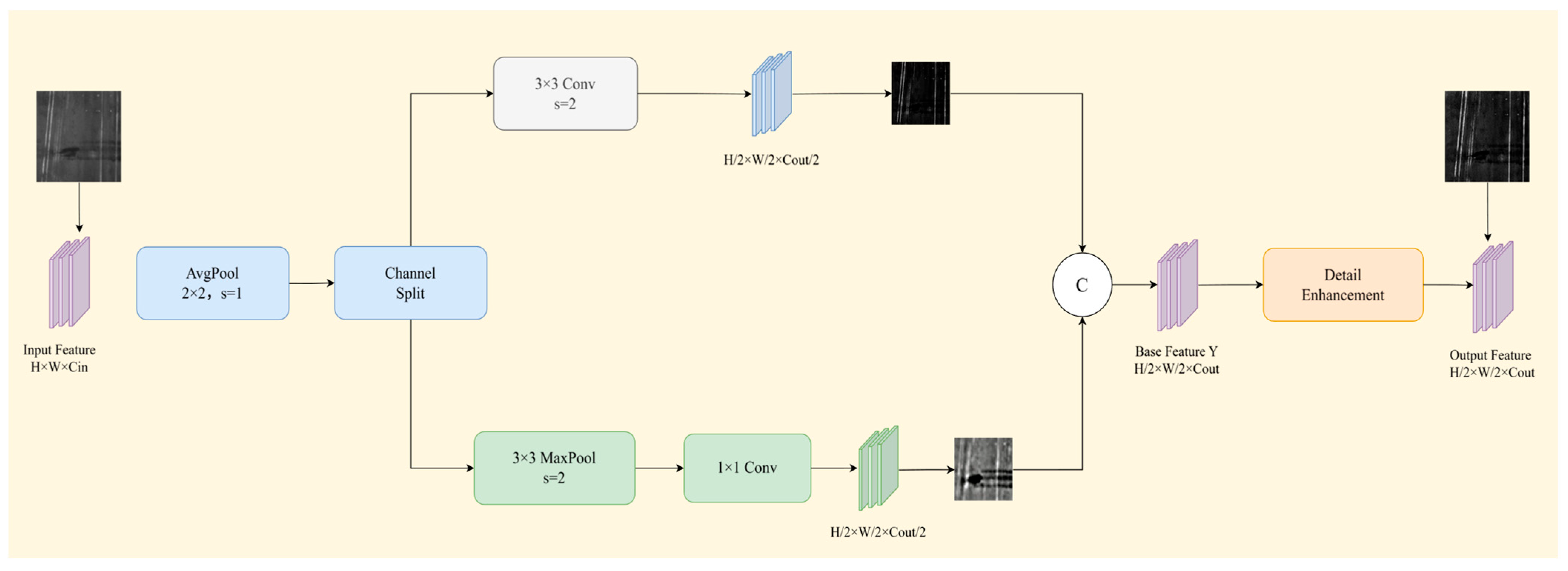
Common detectors often use pooling or strided convolution to reduce feature-map resolution and enlarge the receptive field. Pooling is computationally simple but contains no learnable parameters, whereas strided convolution provides learnable feature extraction but may weaken small-defect, weak-edge, and slender-texture information during downsampling. To address these limitations for steel surfaces, ED-ADown is introduced as a lightweight downsampling module [26]. The module contains a convolution branch and a pooling branch. The former extracts discriminative information with learnable convolutions, and the latter retains local saliency responses. After fusion, the module balances feature learning and fine-detail preservation while limiting the parameter count and computational cost. The input feature first passes through 2 × 2 average pooling for local smoothing, as expressed below:

$$X_{\mathrm{a}}\left(i,j,c\right)={\displaystyle \frac{1}{4}}{\displaystyle \sum _{m=0}^1{\displaystyle \sum _{n=0}^{1}X\left(i+m,j+n,c\right)}}$$

(4)

The average-pooled feature $X_{\mathrm{a}}$ is then divided along the channel dimension into two streams, $X_1$ and $X_2$, which are sent to the convolution branch and the pooling branch, respectively. The convolution branch applies a 3 × 3 convolution with a stride of 2 to $X_1$, thereby extracting local discriminative information from defect regions. This operation is defined as follows:

$$Y_1\left(p,q,k\right)=\delta \left({\displaystyle \sum _c{\displaystyle \sum _{m=-1}^1{\displaystyle \sum _{n=-1}^1{W}_{k,c,m,n}^{\left(1\right)}{X}_1\left(2p+m,2q+n,c\right)+b_k^{\left(1\right)}}}}\right)$$

(5)

In the pooling branch, $X_2$ is first downsampled by a 3 × 3 max-pooling operation with stride 2 to retain salient local responses. A 1 × 1 convolution is then used to adjust the channel dimension, producing the branch output:

$$Y_2\left(p,q,k\right)=\delta \left({\displaystyle \sum _c{W}_{k,c}^{\left(2\right)}Z\left(p,q,c\right)+b_k^{\left(2\right)}}\right)$$

(6)

The two branch outputs are finally concatenated along the channel dimension, and the fused feature is further processed by the detail enhancement unit:

$$Y=\mathrm{Conact}\left(Y_1,Y_2\right)$$

(7)

$$Y_{\mathrm{out}}=F_{\mathrm{DE}}\left(Y\right)$$

(8)

where $X$ denotes the input feature map, $X_{\mathrm{a}}$ denotes the features after average pooling, $X_1$ and $X_2$ are the two feature streams split along the channel dimension, $p$ and $q$ denote the spatial position indices of the output feature maps, $k$ denotes the output channel index, $c$ denotes the input channel index, and $m$ and $n$ denote the spatial offsets of the 3 × 3 convolution kernel, with values ranging from (−1, 0, 1). $W_{k,c,m,n}^{\left(1\right)}$ and $b_k^{\left(1\right)}$ represent the weights and biases of the 3 × 3 convolutional layers, respectively, while $W_{k,c}^{\left(2\right)}$ and $b_k^{\left(2\right)}$ represent the weights and biases of the 1 × 1 convolutional layers, respectively; $\delta \left(·\right)$ denotes a nonlinear activation function. $Z\left(p,q,c\right)$ denotes the feature response obtained from $X_2$ after 3 × 3 max-pooling with a stride of 2. $Y_1$ represents the output feature of the branch obtained by applying a 3 × 3 convolution with a stride of 2 to $X_1$, $Y_2$ denotes the output of the max-pooling and 1 × 1 convolution branches, $Y$ denotes the base downsampled features after merging the two branches, $\mathrm{Conact}\left(·\right)$ denotes concatenation along the channel dimension, $F_{\mathrm{DE}}\left(·\right)$ denotes the detail enhancement unit, and $Y_{\mathrm{out}}$ is the final output feature of the ED-ADown module. Figure 3 shows the structural diagram of the ED-ADown lightweight downsampling module.

As illustrated in Figure 3, ED-ADown completes downsampling through parallel convolutional and pooling branches. The convolution branch retains the learnable feature extraction ability of stride convolution, whereas the pooling branch preserves salient responses around defect regions. After the two streams are concatenated, the spatial size of the feature map is reduced, while small-defect and weak-edge information is better preserved. Therefore, ED-ADown decreases computational cost and improves the retention of fine defects, particularly for crazing and scratches.

3.4. DynamicScalSeq+ASF Module

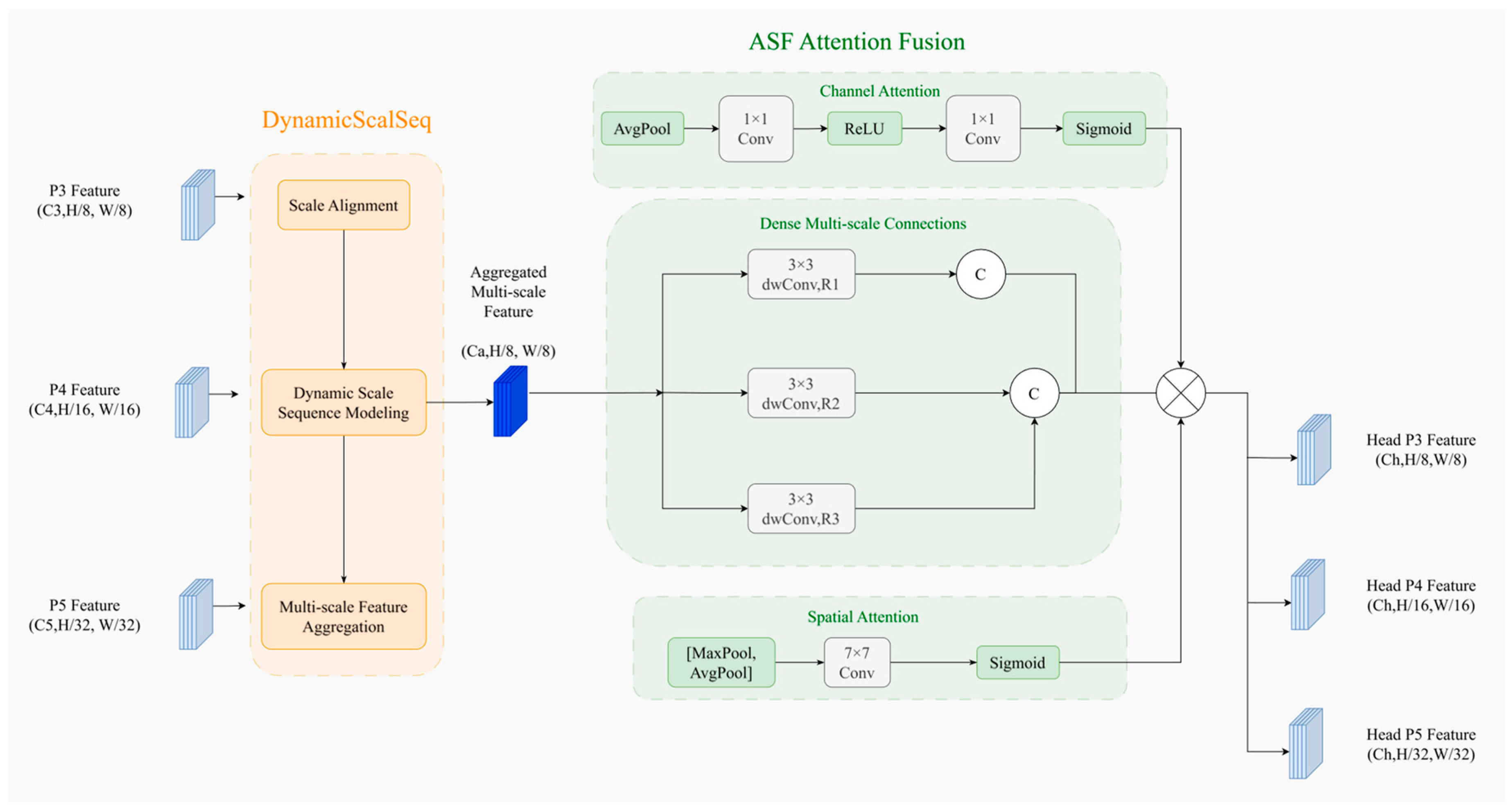
Steel defects vary considerably in scale, morphology, and texture. Shallow features provide detailed edge and texture cues that are useful for locating fine defects such as crazing and scratches, whereas deep features contain stronger semantic information and are better suited to large-area defects such as patches and rolled-in scale. Conventional neck structures often fuse features through fixed routes, making it difficult to adapt to changes in defect size and shape. To overcome this problem, DynamicScalSeq+ASF is introduced as a dynamic multiscale attention fusion module [27,28]. DynamicScalSeq aligns and aggregates P3, P4, and P5 features in a scale-aware manner and assigns adaptive weights to different levels. ASF further strengthens defect-related responses through channel and spatial attention while suppressing background texture interference. The combination of these two components strengthens the interaction between shallow detail cues and deep semantic information, improving the model’s adaptability to multiscale defects with diverse morphologies. The computational process is expressed as follows:

$${\overline{F}}_i=U_i\left(W_i\times F_i\right),i=3,4,5$$

(9)

$$F_{\mathrm{d}}={\displaystyle \sum _{i=3}^5{\omega }_i{\overline{F}}_i}$$

(10)

$$Y=F_{\mathrm{d}}+A_{\mathrm{c}}·F_{\mathrm{d}}+A_{\mathrm{s}}·F_{\mathrm{d}}$$

(11)

where ${\overline{F}}_i$ represents the input features from the i-th scale, (i = 3, 4, 5) corresponding to P3, P4, and P5 features, respectively; $F_i$ represents the scale-aligned features; $U_i\left(·\right)$ represents the upsampling or scale transformation operation; $W_i$ are the learnable weights used for channel adjustment; ${\omega }_i$ are the dynamic fusion weights for the i-th scale features; $F_{\mathrm{d}}$ denotes the multi-scale features aggregated by DynamicScalSeq; $A_{\mathrm{c}}$ represents the channel attention weights; $A_{\mathrm{s}}$ denotes the spatial attention weights; and $Y$ denotes the enhanced features output by the DynamicScalSeq+ASF module. The structural diagram of the DynamicScalSeq+ASF module is shown in Figure 4.

Figure 4 shows that DynamicScalSeq+ASF first performs scale normalization and dynamic aggregation on P3, P4, and P5. The aggregated feature is then refined by the ASF attention fusion structure. By combining shallow detail information with deep semantic cues, the module alleviates the limitations of fixed fusion paths under varying defect scales. For steel surface inspection, this design improves the recognition of small-scale, weak-textured, and morphologically diverse defects.

4. Experiments and Results

4.1. Dataset

The NEU-DET steel surface defect dataset released by Northeastern University was used as the main experimental dataset. It contains 1800 grayscale images covering six defect categories: crazing (Cr), inclusions (In), patches (Pa), pitted surfaces (Ps), rolled-in scale (Rs), and scratches (Sc), with 300 images in each category. Since the public release of NEU-DET does not provide plate, batch, or acquisition-sequence identifiers, a strict source-level partition could not be performed. Therefore, stratified image-level sampling was used to divide the dataset into training, validation, and test sets at a ratio of 8:1:1, yielding 1440, 180, and 180 images, respectively. The class distribution was kept consistent across the three subsets, and the same partition was used for all model comparisons. To evaluate cross-dataset adaptability, the GC10-DET dataset from Tianjin University and the Severstal Steel Defect dataset are also used in the generalization experiments. GC10-DET is divided into 1900 training images and 380 validation images. Since the annotations of the official Severstal test set are unavailable, its 12,568 annotated images are divided into 10,054 training images, 1257 validation images, and 1257 test images. These datasets help evaluate the model under more complex textures, different defect distributions, and varying imaging conditions.

4.2. Experimental Setup

All experiments were conducted on Windows 11 using an NVIDIA GeForce RTX 3060 GPU with 6 GB VRAM and an Intel Core i9-12900H CPU, with CUDA 11.8 and PyTorch 2.7.1. The models were initialized with YOLO11n pretrained weights and trained for 200 epochs at 512 × 512 resolution with a batch size of 16. AdamW was adopted with an initial learning rate of 0.0004, a weight decay of 0.002, a five-epoch warm-up, cosine scheduling, and an early-stopping patience of 50 epochs. Mosaic, horizontal flipping, and vertical flipping were applied with probabilities of 0.35, 0.5, and 0.3, respectively. Five random seeds (0, 1, 2, 3, and 4) were used for repeated experiments. During evaluation, the confidence and NMS IoU thresholds were set to 0.25 and 0.7. The default YOLO11 loss gains for box regression, classification, and DFL were 7.5, 0.5, and 1.5. Inference was performed in FP32 with a batch size of 1 and without test-time augmentation.

4.3. Evaluation Metrics

Model performance is evaluated using Precision, Recall, mAP50, mAP50–95, Params, GFLOPs, and FPS. The corresponding calculation formulas are given below.

$$\mathrm{Precision}={\displaystyle \frac{T_{\mathrm{p}}}{T_{\mathrm{p}}+F_{\mathrm{p}}}}$$

(12)

$$\mathrm{Recall}={\displaystyle \frac{T_{\mathrm{p}}}{T_{\mathrm{p}}+F_{\mathrm{n}}}}$$

(13)

$$\mathrm{AP}={\displaystyle {\int }_0^1\mathrm{Precision}}\left(\mathrm{Recall}\right)d\left(\mathrm{Recall}\right)$$

(14)

$$\mathrm{mAP}={\displaystyle \frac{1}{n}}{\displaystyle \sum _{i=0}^n\mathrm{AP}\left(i\right)}$$

(15)

$$\mathrm{FPS}={\displaystyle \frac{\mathrm{Framenum}}{\mathrm{Elapsedtime}}}$$

(16)

In the formula, $T_{\mathrm{p}}$ represents the number of correctly detected defect targets, $F_{\mathrm{p}}$ represents the number of false positives, $F_{\mathrm{n}}$ represents the number of false negatives, $\mathrm{Precision}$ represents the proportion of true defects among targets predicted to be defects, and $\mathrm{Recall}$ represents the proportion of true defects that were correctly detected. $\mathrm{Framenum}$ is the total number of images to be inspected, and $\mathrm{Elapsedtime}$ is the time required to inspect all images.

4.4. Ablation Experiments

To evaluate the influence of the proposed components, ablation experiments were carried out on the NEU-DET dataset [29]. The experiments consisted of two parts. The first part examined different parameter settings and analyzed their influence on accuracy and computational efficiency. The second part added the modules step by step to measure their respective contributions to the final network. All experiments used the same dataset split, input size, training protocol, and evaluation metrics to ensure fair comparison.

4.4.1. Parameter Ablation Experiment for the C3k2-TFE-EMA Module

C3k2-TFE-EMA is designed to improve the ability of the backbone to extract texture-related defect features. Through the texture frequency-domain enhancement branch and EMA attention, the module increases the response to low-contrast regions. Because the weight of the texture frequency-domain branch controls how strongly the model attends to local details and background textures, different enhancement weights are tested in the parameter ablation study. Given an input feature, the output of the C3k2-TFE-EMA module is formulated as:

$$Y=F_{\mathrm{base}}\left(X\right)+\lambda F_{\mathrm{tfe}}\left(X\right)$$

(17)

$$F_{\mathrm{base}}\left(X\right)=F_{\mathrm{C}3\mathrm{k}2}\left(X\right)+F_{\mathrm{ema}}\left(X\right)$$

(18)

where $F_{\mathrm{C}3\mathrm{k}2}\left(X\right)$ represents the output feature of the C3k2 main branch, $F_{\mathrm{tfe}}\left(X\right)$ represents the output feature of the texture frequency-domain enhancement branch, $F_{\mathrm{ema}}\left(X\right)$ represents the EMA attention-enhanced feature, $F_{\mathrm{base}}\left(X\right)$ denotes the base enhanced features obtained by fusing the C3k2 main branch with the EMA attention branch, and $\lambda$ is the fusion weight of the texture frequency-domain branch. A small $\lambda$ limits the use of frequency-domain texture information, whereas an excessively large $\lambda$ may amplify local texture fluctuation and background noise. Therefore, the best-performing value among the tested settings was determined experimentally. The parameter ablation results for C3k2-TFE-EMA are given in

Table 1. Results of the C3k2-TFE-EMA module parameter ablation experiment.

Model	λ	P%	R%	mAP50%	Params/M	GFLOPs	FPS
YOLO11n	-	69.7	73.3	74.2	2.583	6.3	164.8
+C3k2-TFE-EMA	0.25	70.8	72.5	76.2	2.585	6.4	161.9
+C3k2-TFE-EMA	0.50	71.5	74.2	77.5	2.585	6.4	161.6
+C3k2-TFE-EMA	0.75	72.0	74.6	78.3	2.585	6.4	161.4

.

Table 1 shows the influence of λ on the performance of C3k2-TFE-EMA. At λ = 0.25, Precision and mAP50 increase to 70.8% and 76.2%, respectively, whereas Recall decreases from 73.3% to 72.5%, indicating that a relatively small frequency-domain contribution provides limited benefit for reducing missed detections. Increasing λ to 0.50 raises Recall and mAP50 to 74.2% and 77.5%. Among the tested settings, λ = 0.75 achieves the highest Precision, Recall, and mAP50 of 72.0%, 74.6%, and 78.3%, respectively. Compared with YOLO11n, Recall increases by 1.3 percentage points and mAP50 by 4.1 percentage points, while the parameters and GFLOPs increase only slightly from 2.583 M and 6.3 to 2.585 M and 6.4. The FPS decreases slightly from 164.8 to 161.4. Since missed defects may have more serious consequences than false alarms in industrial inspection, λ = 0.75 was selected as a recall-aware balance between defect coverage, detection accuracy, and computational efficiency.

4.4.2. Parameter Ablation Experiment for the DynamicScalSeq+ASF Module

DynamicScalSeq+ASF is used in the neck to improve multiscale feature fusion. DynamicScalSeq performs scale alignment and dynamic sequence modeling on the P3, P4, and P5 features. ASF then refines the fused feature through channel attention, spatial attention, and dense multiscale connections. The number of fusion channels affects both feature representation and computational cost, so parameter ablation is conducted for this setting. Given the multiscale input features $F_3$, $F_4$, and $F_5$, the output of DynamicScalSeq can be expressed as:

$$Y_{\mathrm{asf}}=\mathrm{ASF}\left(\mathrm{DSS}\left(F_3,F_4,F_5;C_f\right)\right)$$

(19)

where $Y_{\mathrm{asf}}$ represents the output features after dynamic multiscale attention fusion; $F_3$, $F_4$, and $F_5$ represent the input features from layers P3, P4, and P5, respectively; $\mathrm{DSS}\left(·\right)$ denotes the DynamicScalSeq dynamic scale sequence modeling operation, which is used to perform multiscale feature alignment and correlation modeling; and $\mathrm{DSS}\left(·\right)$ denotes the adaptive spatial feature fusion operation, which is used to further enhance the channel and spatial expressiveness of the fused features. $C_f$ denotes the number of fused channels. A smaller value of $C_f$ reduces computational complexity but may limit multiscale feature representation; a larger value of $C_f$ enhances feature representation but increases computational complexity. The results of the parameter ablation experiments for the DynamicScalSeq+ASF module are shown in

Table 2. Results of the DynamicScalSeq+ASF module parameter ablation experiments.

Model	Cf	P%	R%	mAP50%	Params/M	GFLOPs	FPS
YOLO11n+C3k2-TFE-EMA+ED-ADown	-	71.3	76.7	78.1	2.088	5.1	181.6
+DynamicScalSeq+ASF	128	76.6	73.2	78.5	2.096	5.2	178.3
+DynamicScalSeq+ASF	256	78.3	73.6	79.0	2.106	5.3	175.5
+DynamicScalSeq+ASF	512	76.8	74.0	78.7	2.137	5.6	168.9

.

According to Table 2, adding DynamicScalSeq+ASF to the C3k2-TFE-EMA and ED-ADown model further improves mAP50. When $C_f$ is set to 128, Precision and mAP50 reach 76.6% and 78.5, respectively, which are higher than the results obtained without this module. This confirms that DynamicScalSeq+ASF strengthens communication among features at different scales. With $C_f$ = 256, the model obtains the best overall performance, achieving 78.3% Precision, 73.6% Recall, and 79.0% mAP50, while using only 2.106 M parameters and 5.3 GFLOPs with 175.5 FPS. When $C_f$ increases to 512, Recall rises to 74.0%, but mAP50 drops to 78.7%, and the parameters and GFLOPs increase to 2.137 M and 5.6, respectively. These results suggest that too many fusion channels introduce redundant information and extra computation. Therefore, $C_f$ = 256 is used as the default configuration.

4.4.3. Progressive Ablation Experiments

To further verify the contribution of each component, seven groups of ablation experiments were conducted on the NEU-DET dataset. Starting from YOLO11n, T-YOLO11n is obtained by adding only C3k2-TFE-EMA, A-YOLO11n by adding only ED-ADown, and D-YOLO11n by adding only DynamicScalSeq+ASF. TA-YOLO11n combines C3k2-TFE-EMA and ED-ADown, TD-YOLO11n combines C3k2-TFE-EMA and DynamicScalSeq+ASF, and AD-YOLO11n combines ED-ADown and DynamicScalSeq+ASF. Finally, all three modules are integrated to form TAD-YOLO11n. The results are shown in

Table 3. Results of the progressive ablation experiments.

Model	P%	R%	mAP50%	mAP50–95/%	Params/M	GFLOPs	FPS
YOLO11n	69.7	73.3	74.2	43.1	2.583	6.3	164.8
T-YOLO11n	72.0	74.6	78.3	45.2	2.585	6.4	161.4
A-YOLO11n	70.5	75.7	76.1	43.6	2.086	5.1	183.3
D-YOLO11n	73.1	73.9	77.4	43.8	2.594	6.4	160.7
TA-YOLO11n	71.3	76.7	78.1	44.2	2.088	5.1	181.6
TD-YOLO11n	76.1	74.5	78.6	45.1	2.596	6.5	157.9
AD-YOLO11n	75.9	74.4	77.8	44.5	2.104	5.2	177.3
TAD-YOLO11n	78.3	73.6	79.0	45.3	2.106	5.3	175.5

.

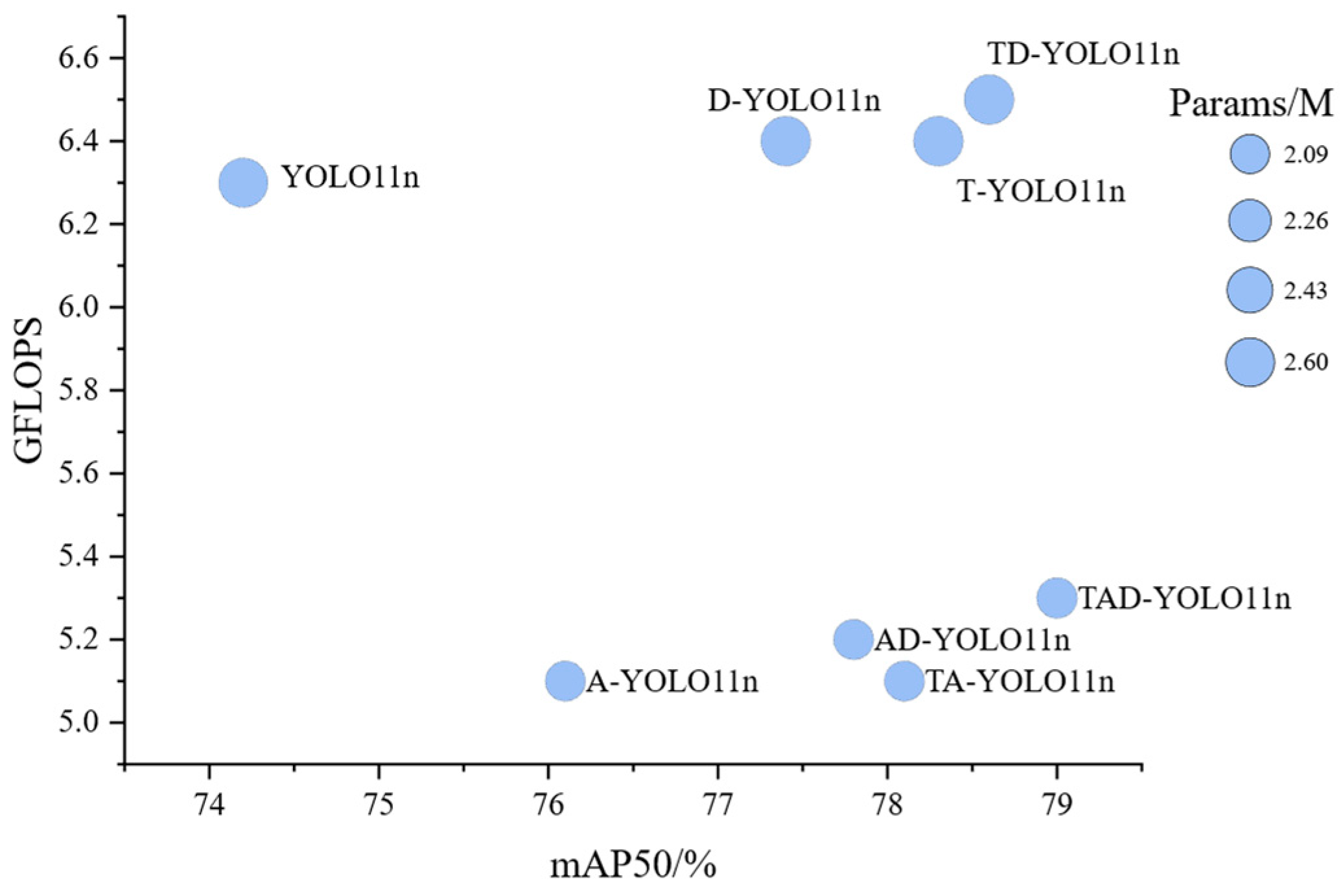
The results in Table 3 demonstrate the effectiveness of the proposed modules. After introducing C3k2-TFE-EMA, T-YOLO11n improves mAP50 and mAP50–95 from 74.2% and 43.1% to 78.3% and 45.2%, respectively, indicating stronger representation of weak-texture and low-contrast defects. The module introduces only limited computational overhead, as reflected by the slight decrease in FPS from 164.8 for YOLO11n to 161.4 for T-YOLO11n. After ED-ADown is introduced, A-YOLO11n reduces the number of parameters from 2.583 M to 2.086 M and the computational cost from 6.3 to 5.1 GFLOPs while increasing FPS to 183.3. This result shows that ED-ADown effectively reduces redundant computation during downsampling. Adding DynamicScalSeq+ASF alone increases the mAP50 of D-YOLO11n to 77.4%, demonstrating improved cross-scale feature interaction. Among the combined configurations, TA-YOLO11n achieves the highest Recall of 76.7%, indicating that texture enhancement and detail-preserving downsampling complement each other in detecting defect targets. TD-YOLO11n achieves an mAP50 of 78.6%, although its parameters and computational cost increase to 2.596 M and 6.5 GFLOPs, respectively. The complete TAD-YOLO11n achieves the highest Precision, mAP50, and mAP50–95, reaching 78.3%, 79.0%, and 45.3%, respectively. Compared with YOLO11n, its mAP50 and mAP50–95 increase by 4.8 and 2.2 percentage points, while the parameters and computational cost decrease to 2.106 M and 5.3 GFLOPs. The model also achieves an inference speed of 175.5 FPS. Therefore, the additional cost of the frequency-domain operation is offset by the computational reduction introduced by the lightweight downsampling path, allowing TAD-YOLO11n to improve detection accuracy without sacrificing inference efficiency. Figure 5 presents the corresponding accuracy complexity analysis.

Figure 5 indicates that T-YOLO11n, D-YOLO11n, and TD-YOLO11n obtain higher mAP50 than YOLO11n, although their GFLOPs are also increased. In contrast, A-YOLO11n, TA-YOLO11n, and AD-YOLO11n reduce GFLOPs, confirming the computational advantage of ED-ADown. TAD-YOLO11n achieves 79.0% mAP50 with 5.3 GFLOPs, indicating that the proposed model improves accuracy while reducing computational cost compared with the baseline.

4.5. Repeated Experiments and Statistical Stability

To reduce the influence of random initialization, data shuffling, and stochastic augmentation, the YOLO11n baseline and TAD-YOLO11n were independently trained using five random seeds: 0, 1, 2, 3, and 4. The same dataset split, hyperparameters, and hardware environment were used in all repeated experiments. The repeated experimental results of YOLO11n and TAD-YOLO11n under the five random seeds are shown in

Table 4. Repeated experimental results of YOLO11n and TAD-YOLO11n under five random seeds.

Model	P%	R%	mAP50%	mAP50–95/%
YOLO11n	69.7 ± 0.5	73.1 ± 0.7	74.1 ± 0.4	43.1 ± 0.3
TAD-YOLO11n	78.2 ± 0.4	73.8 ± 0.5	79.0 ± 0.2	45.3 ± 0.3

.

As shown in Table 4, TAD-YOLO11n achieved an average mAP50 of 79.0% ± 0.2%, compared with 74.1% ± 0.4% for YOLO11n. The improvement was consistently observed across the five runs, indicating that the reported performance gain was not caused by a favorable random initialization. In addition, the relatively small standard deviation demonstrates the training stability of the proposed model.

4.6. Evaluation Under Different Random Dataset Splits

To reduce the dependence of the results on a single dataset partition, five stratified random splits of NEU-DET were generated using split seeds of 0, 1, 2, 3, and 4. For each split, the dataset was divided into training, validation, and test sets at a ratio of 8:1:1. YOLO11n and TAD-YOLO11n were trained and evaluated using the same partition in each run, while the training seed and all other experimental settings were kept fixed. The averaged results are presented in

Table 5. Results of YOLO11n and TAD-YOLO11n over five stratified random splits of NEU-DET.

Model	P%	R%	mAP50%	mAP50–95/%
YOLO11n	69.3 ± 0.8	72.7 ± 1.0	73.8 ± 0.7	42.8 ± 0.6
TAD-YOLO11n	77.9 ± 0.7	73.4 ± 0.8	78.6 ± 0.6	45.0 ± 0.5

.

As shown in Table 5, TAD-YOLO11n achieves better average performance than YOLO11n over the five stratified random splits. Its average mAP50 and mAP50–95 reach 78.6% ± 0.6% and 45.0% ± 0.5%, respectively, compared with 73.8% ± 0.7% and 42.8% ± 0.6% for YOLO11n. The proposed model maintains its performance advantage under different dataset partitions, indicating that the improvement is not dependent on a particular train–validation–test split.

4.7. Comparative Experiments

To verify the advantages of TAD-YOLO11n, the proposed model was compared with several representative detectors under the same experimental conditions, including YOLO11n, YOLO26n, D-FINE, YOLO11n, and RT-DETR-R18. For a fair comparison, all models used the same NEU-DET training, validation, and test split. The input size, training epochs, batch size, evaluation metrics, and hardware platform were also kept consistent. Models with available pretrained weights were initialized with the corresponding official weights, whereas models without the same pretrained setting followed their default configurations. Except for architectural differences, augmentation strategies, optimizers, and major hyperparameters were kept as consistent as possible to reduce the influence of non-architectural factors. The comparison results are presented in

Table 6. Comparative experiments of various common object detection algorithms.

Model	P%	R%	mAP50%	mAP50–95/%	Params/M	GFLOPs	FPS
YOLO11n	69.7	73.3	74.2	43.1	2.583	6.3	164.8
YOLO26n	68.1	71.6	74.1	42.1	2.387	5.2	178.3
DFINE	70.4	67.0	73.5	42.7	3.865	7.4	132.5
YOLOv10n	70.8	72.6	73.7	42.9	2.574	6.2	165.1
RT-DETR-R18	74.5	70.5	72.6	41.5	20.54	61.8	63.7
TAD-YOLO11n	78.3	73.6	79.0	45.3	2.106	5.3	175.5

[30].

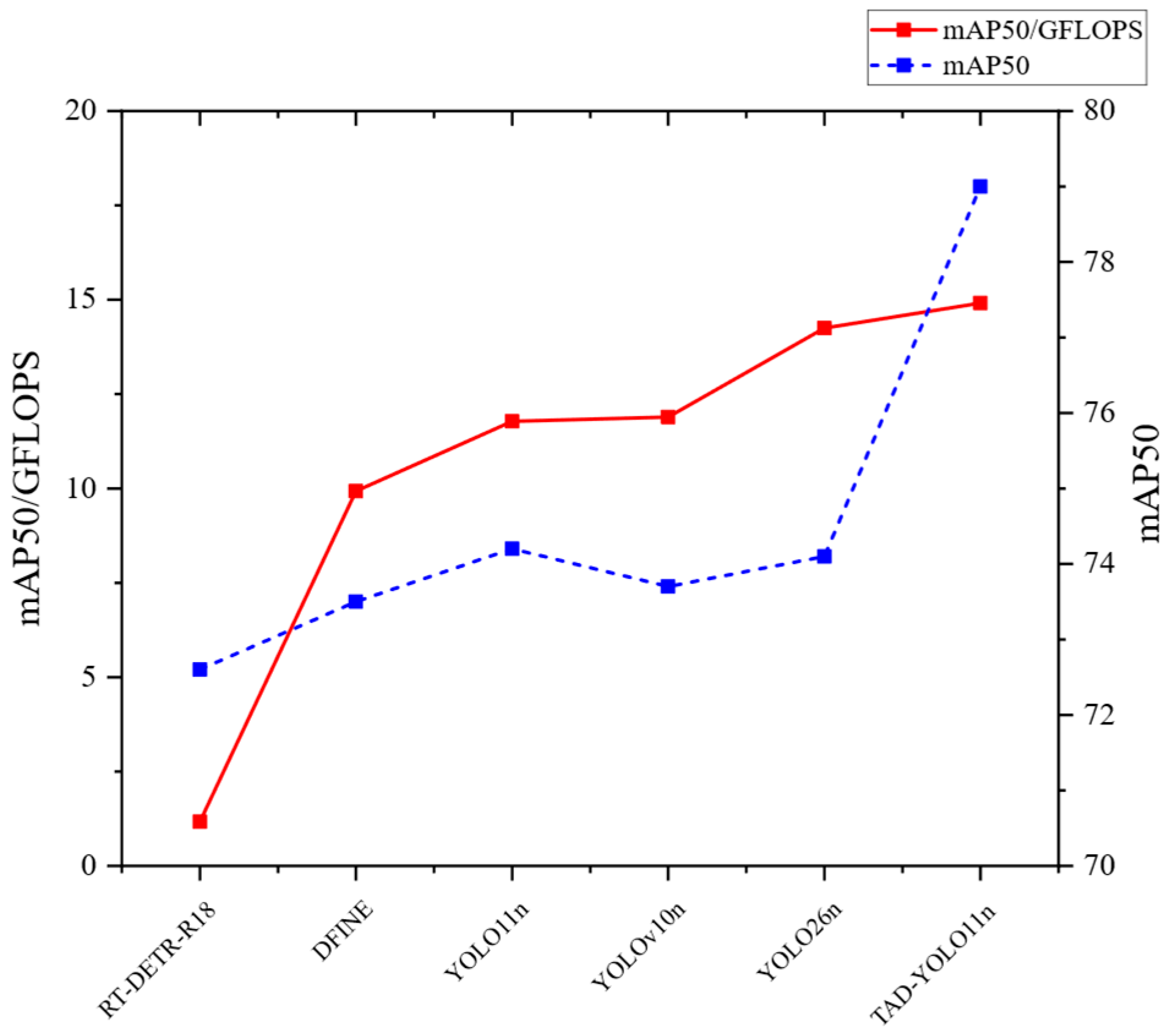
As shown in Table 6, TAD-YOLO11n achieves the best overall detection performance among the compared models, with Precision, Recall, mAP50, and mAP50–95 reaching 78.3%, 73.6%, 79.0%, and 45.3%, respectively. Compared with YOLO11n, TAD-YOLO11n improves mAP50 and mAP50–95 by 4.8 and 2.2 percentage points while reducing the number of parameters from 2.583 M to 2.106 M and GFLOPs from 6.3 to 5.3. Its inference speed also increases from 164.8 to 175.5 FPS. Compared with YOLOv10n, TAD-YOLO11n improves Precision, Recall, mAP50, and mAP50–95 by 7.5, 1.0, 5.3, and 2.4 percentage points, respectively, with fewer parameters and lower computational cost. Compared with RT-DETR-R18, the proposed model increases mAP50 and mAP50–95 by 6.4 and 3.8 percentage points while reducing the parameters from 20.54 M to 2.106 M and GFLOPs from 61.8 to 5.3. Its FPS is also substantially higher than the 63.7 FPS of RT-DETR-R18. These results show that TAD-YOLO11n provides a favorable balance among detection accuracy, model complexity, and inference speed. Figure 6 further compares the accuracy computation ratio of different models.

Figure 6 further illustrates the relationship between detection accuracy and computational cost. TAD-YOLO11n achieves the highest mAP50/GFLOPs ratio of 14.91, together with the best mAP50 of 79.0%, indicating that its accuracy improvement is obtained without increasing computational burden. Although YOLO26n also shows a relatively high efficiency ratio, its detection accuracy remains lower than that of TAD-YOLO11n. By contrast, RT-DETR-R18 requires substantially more computation, resulting in a much lower accuracy–efficiency ratio. Overall, TAD-YOLO11n provides a more favorable trade-off between detection performance and model complexity. The category-level detection results are presented in

Table 7. Class-wise AP50 comparison of different object detectors on the NEU-DET dataset.

Model	AP50%
	Cr	In	Pa	Ps	Rs	Sc
YOLO11n	33.2	78.2	93.1	92.2	55.7	92.9
YOLO26n	35.3	75.8	91.6	89.3	56.4	91.5
DFINE	39.4	76.3	90.7	87.4	54.7	87.7
YOLOv10n	44.5	72.6	89.2	86.7	60.8	88.4
RT-DETR-R18	40.2	73.5	87.8	89.4	58.1	86.5
TAD-YOLO11n	43.1	81.7	94.3	91.5	66.4	96.7

.

Table 7 shows that TAD-YOLO11n improves the AP50 of most defect categories compared with YOLO11n. For crazing (Cr), the AP50 increases from 33.2% to 43.1%. Despite this improvement, its performance remains lower than that of the other categories, mainly because crazing defects are often thin, discontinuous, and low in contrast, making them difficult to distinguish from background textures and scratches. For scratches (Sc), the AP50 increases from 92.9% to 96.7%, suggesting that ED-ADown preserves fine elongated features during downsampling. The model also achieves the highest mAP50 for inclusions, patches, rolled-in scale, and scratches, confirming the effectiveness of multiscale feature fusion.

4.8. Visualization Analysis

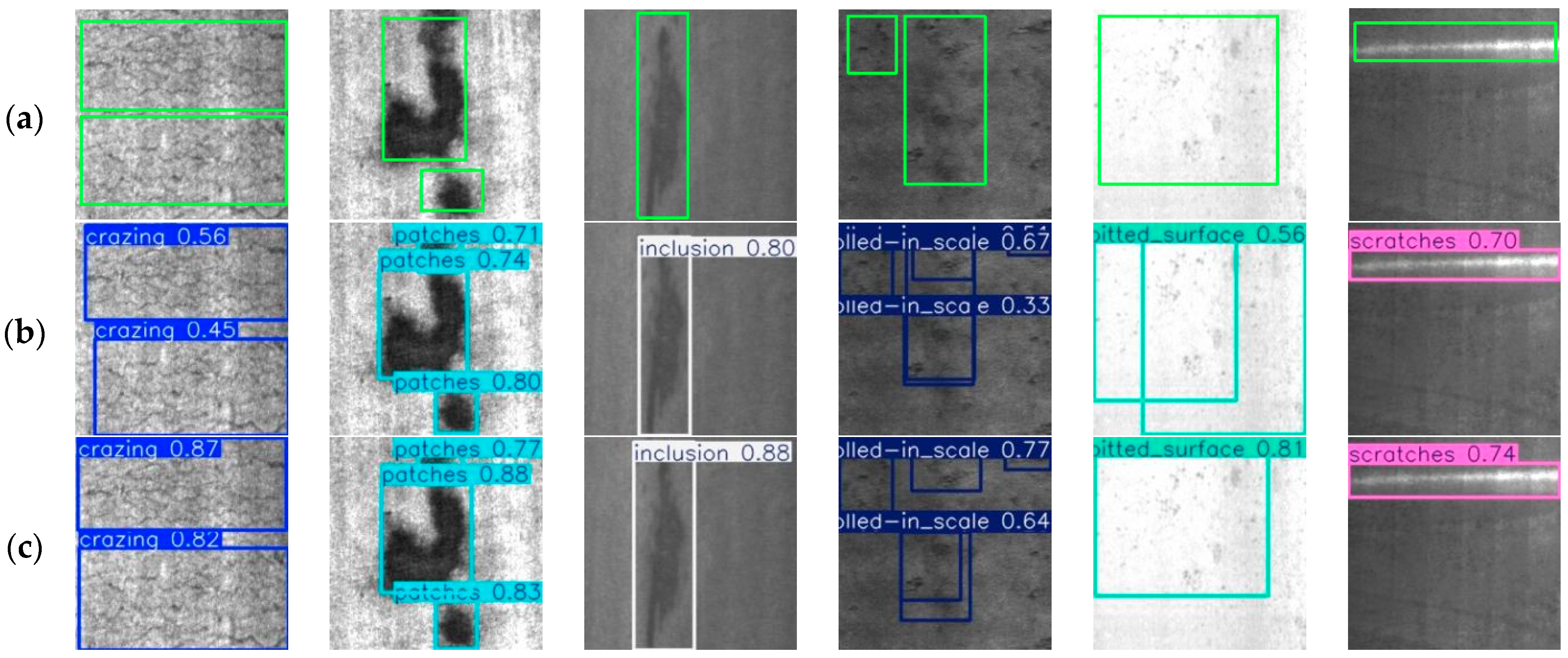
To provide an intuitive comparison between the proposed detector and YOLO11n, detection results on the NEU-DET dataset are visualized in Figure 7.

Figure 7 shows that YOLO11n can detect most steel surface defects, but it produces relatively low confidence scores for weak-textured or blurred-boundary categories, such as crazing, rolled-in scale, and pitted surfaces. In comparison, TAD-YOLO11n improves the detection confidence for several defect categories. For crazing defects, the confidence scores increase from 0.56 and 0.45 to 0.87 and 0.82, respectively. For rolled-in scale, they increase from 0.67 and 0.33 to 0.77 and 0.64. For pitted surfaces, the confidence score increases from 0.56 to 0.81, while that of inclusions increases from 0.80 to 0.88. These results indicate that the proposed model captures texture, edge, and multiscale information more effectively, thereby improving the recognition of low-contrast and complex-textured defects.

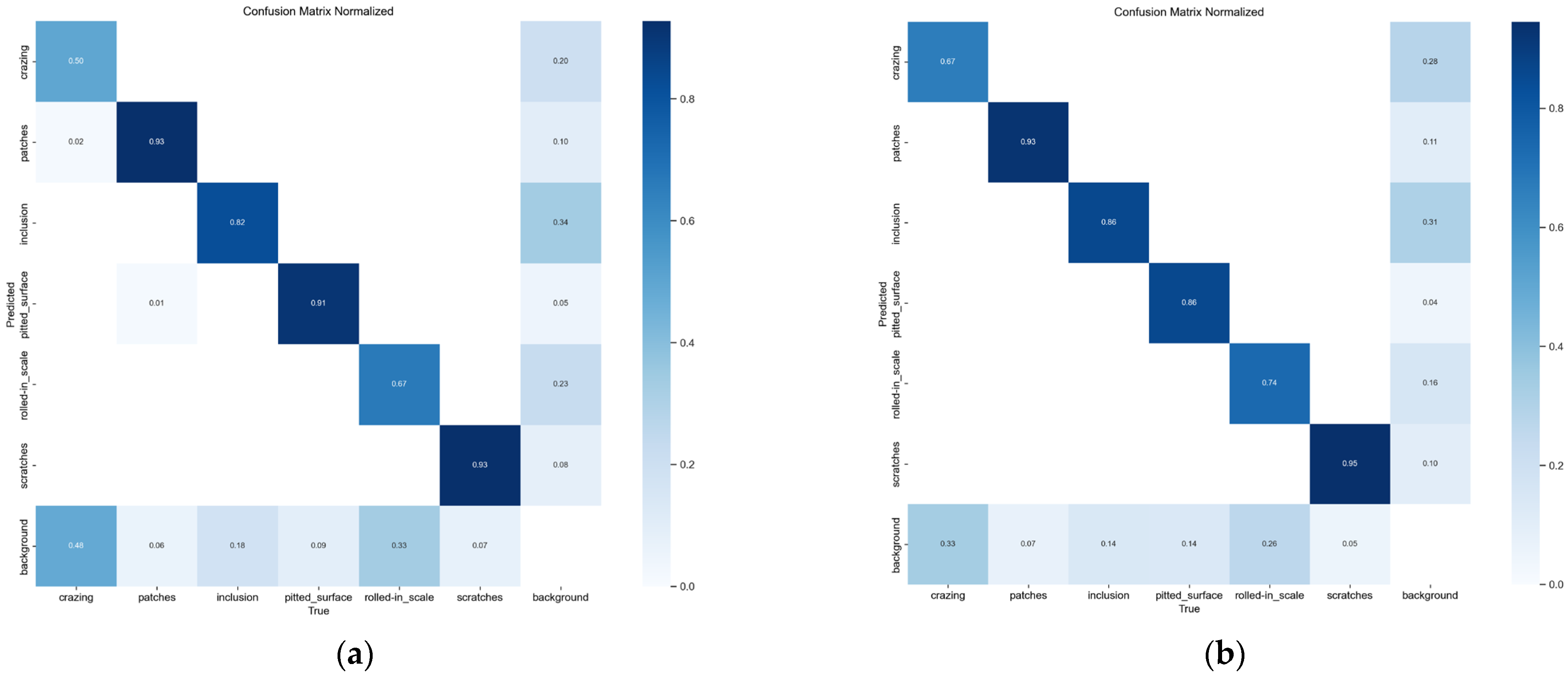
To provide a quantitative analysis of class-wise recognition and background-related errors, the normalized confusion matrices of YOLO11n and TAD-YOLO11n are further presented in Figure 8.

As shown in Figure 8, TAD-YOLO11n improves the normalized diagonal values for most defect categories compared with YOLO11n. The recognition rates of crazing, inclusions, rolled-in scale, and scratches increase from 0.50, 0.82, 0.67, and 0.93 to 0.67, 0.86, 0.74, and 0.95, respectively. In particular, the proportion of crazing and rolled-in scale defects classified as background decreases from 0.48 and 0.33 to 0.33 and 0.26, indicating fewer missed detections of weak-textured defects. The recognition rate of patches remains unchanged at 0.93, whereas that of pitted surface decreases slightly from 0.91 to 0.86. Overall, TAD-YOLO11n improves the recognition of most defect categories, although the degree of improvement varies across classes. The experimental training curves before and after the improvements are shown in Figure 9.

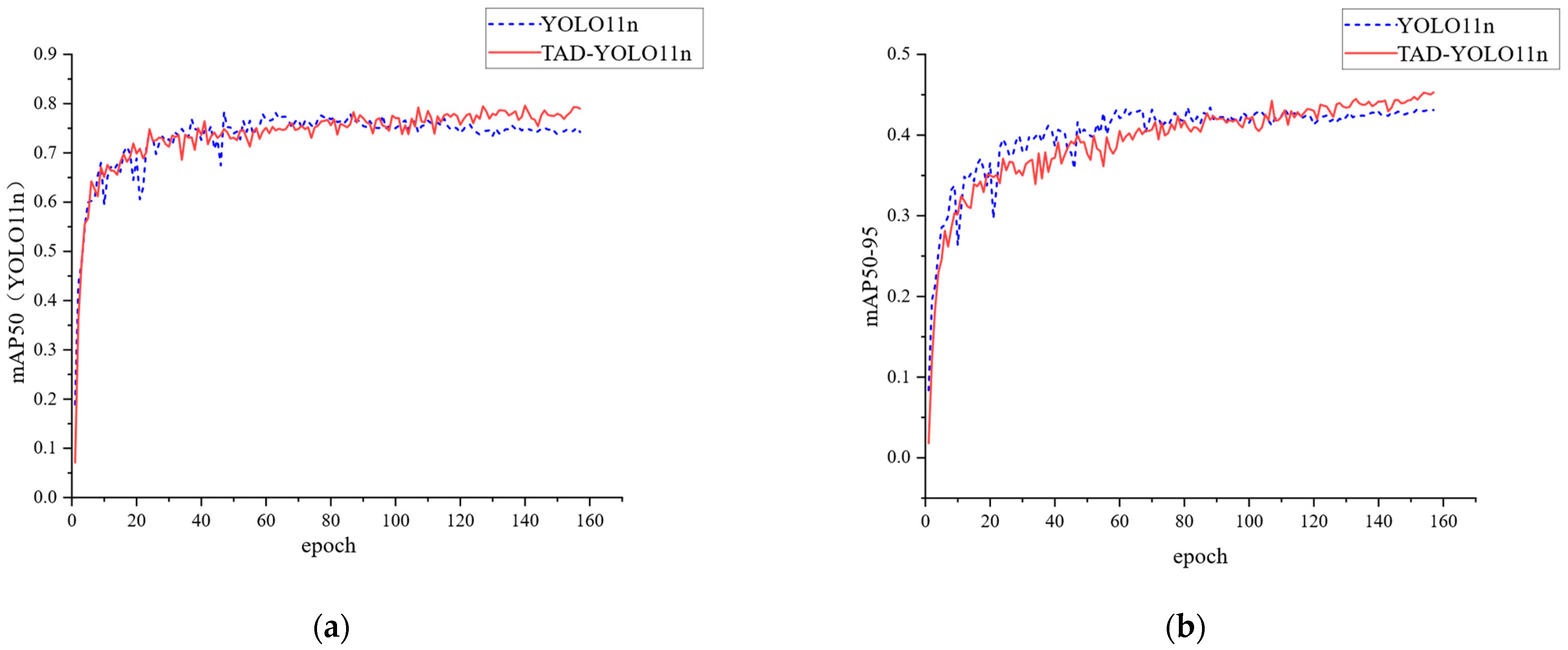
Figure 9 demonstrates that the mAP50 and mAP50–95 curves of both YOLO11n and TAD-YOLO11n rise quickly in the early training stage and then gradually become stable. TAD-YOLO11n remains at a higher level during the later training stage. Its final mAP50 reaches 79.0%, compared with 74.2% for YOLO11n, and its mAP50–95 reaches 45.3%, compared with 43.1% for YOLO11n. This indicates that the improved network enhances both defect detection accuracy and localization ability while maintaining stable convergence.

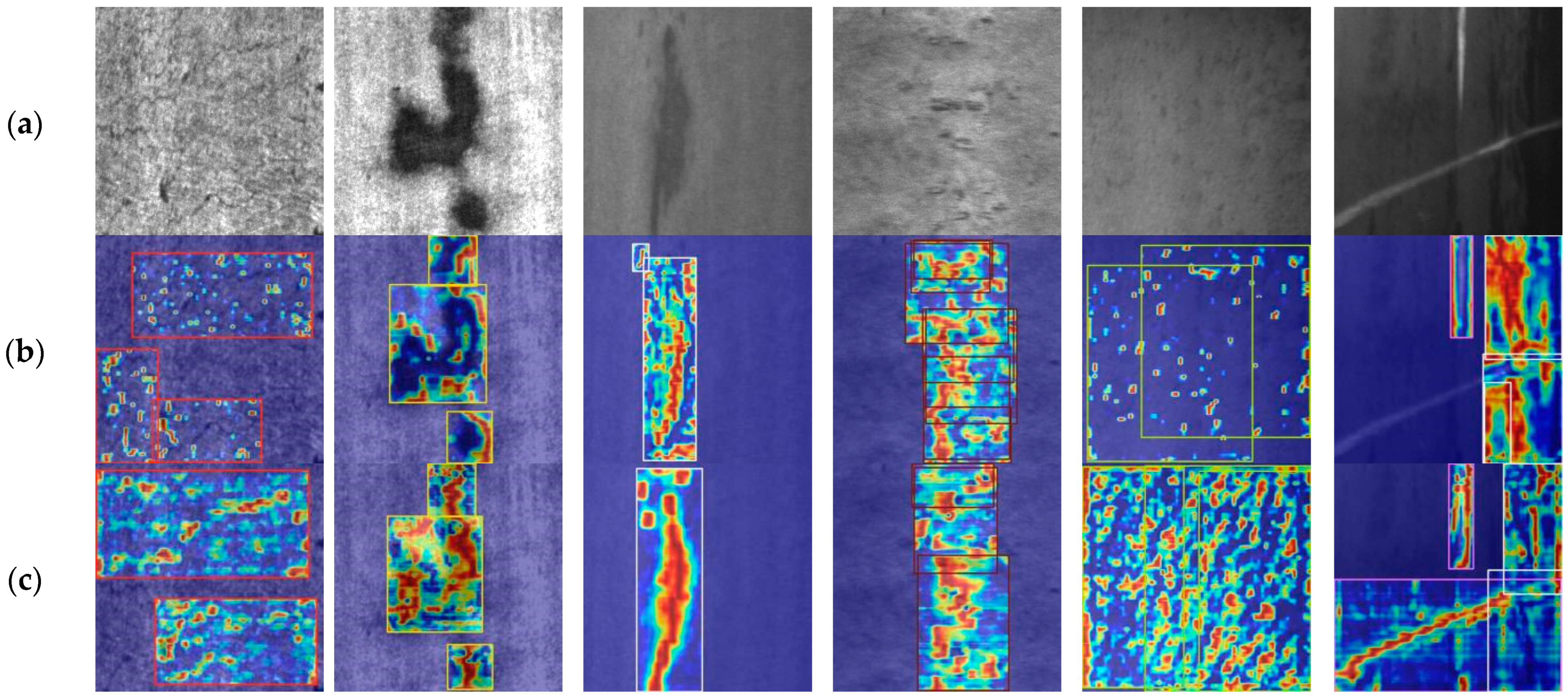
Grad-CAM is further used to analyze how different models respond to defect regions, and the visualization results are shown in Figure 10.

As presented in Figure 10, the heatmap responses of YOLO11n are relatively scattered, and some high-response areas deviate from the real defect positions. This suggests that the baseline model does not focus sufficiently on key defect cues. In comparison, TAD-YOLO11n produces more concentrated responses around the main defect areas and shows less interference from the background. The visualization results indicate that the proposed improvements enhance feature extraction in defect regions and improve localization stability.

4.9. Generalization Experiments

To further evaluate the adaptability of TAD-YOLO11n across different industrial defect datasets, additional experiments were conducted on GC10-DET and the Severstal Steel Defect dataset. These datasets differ from NEU-DET in defect categories, image characteristics, and data distributions. YOLO11n and TAD-YOLO11n were separately trained and evaluated on each dataset using the same data split and training settings. The experiments examined whether the proposed improvements remained effective under different industrial inspection conditions.

4.9.1. Evaluation on GC10-DET

GC10-DET contains more diverse defect categories and more complex background textures than NEU-DET. All models were retrained using the GC10-DET training set, while the main training settings were kept consistent with those used on NEU-DET. The comparative results are presented in

Table 8. Performance comparison of different object detectors on the GC10-DET dataset.

Model	P%	R%	mAP50%	mAP50–95/%	Params/M	GFLOPs	FPS
YOLO11n	65.8	68.9	70.4	39.2	2.587	6.4	162.6
YOLO26n	66.5	66.8	69.6	38.4	2.391	5.3	175.1
DFINE	69.2	62.7	70.9	39.0	3.872	7.5	130.9
YOLOv10n	67.8	67.2	70.7	39.4	2.329	6.7	158.4
RT-DETR-R18	71.0	58.7	70.6	38.8	20.03	57.2	49.6
TAD-YOLO11n	73.6	70.1	74.8	41.6	2.110	5.4	173.2

.

As shown in Table 8, TAD-YOLO11n maintains its performance advantage on GC10-DET. Compared with YOLO11n, its Precision, Recall, mAP50, and mAP50–95 increase by 7.8, 1.2, 4.4, and 2.4 percentage points, respectively. TAD-YOLO11n also uses fewer parameters and lower computational cost while achieving a higher inference speed. These results indicate that the proposed improvements remain effective for defect categories and background textures different from those in NEU-DET.

4.9.2. Evaluation on the Severstal Steel Defect Dataset

The Severstal Steel Defect dataset was further introduced to evaluate the adaptability of the proposed model to steel images collected under different imaging conditions. The original pixel-level annotations were converted into bounding boxes for object detection. YOLO11n and TAD-YOLO11n were trained and evaluated using the same dataset split and experimental settings. The results are shown in

Table 9. Detection results of YOLO11n and TAD-YOLO11n on the Severstal Steel Defect dataset.

Model	P%	R%	mAP50%	mAP50–95/%	Params/M	GFLOPs	FPS
YOLO11n	59.2	53.8	50.1	26.9	2.581	6.3	165.2
TAD-YOLO11n	62.7	56.4	54.2	29.7	2.104	5.3	176.4

.

As shown in Table 9, TAD-YOLO11n achieves higher Precision, Recall, mAP50, and mAP50–95 than YOLO11n on the Severstal Steel Defect dataset, with improvements of 3.5, 2.6, 4.1, and 2.8 percentage points, respectively. The consistent performance gains on Severstal further demonstrate that the proposed texture enhancement, detail-preserving downsampling, and multiscale feature fusion strategies are not limited to NEU-DET or GC10-DET.

Overall, TAD-YOLO11n consistently outperforms the YOLO11n baseline on NEU-DET, GC10-DET, and the Severstal Steel Defect dataset. Although the performance gains vary across datasets, the proposed model maintains a favorable accuracy–complexity balance under different defect categories and image distributions, demonstrating its adaptability to diverse steel surface inspection scenarios.

4.10. Robustness Evaluation Under Image Degradation

To evaluate the robustness of the proposed model under common image degradation conditions, Gaussian noise, lighting shifts, and Gaussian blur were applied to the original NEU-DET test set without changing the annotations. Three severity levels were considered for each degradation type. Gaussian noise was generated with standard deviations of 10, 20, and 30. Lighting variations of ±20%, ±40%, and ±60% were applied, and the results obtained under darker and brighter conditions were averaged at each level. Gaussian blur was introduced using kernel sizes of 3 × 3, 5 × 5, and 7 × 7. The trained models were evaluated directly on the degraded test sets without further training, using the same evaluation settings as for the original test set. The experimental results are shown in

Table 10. Robustness comparison under different image degradation conditions.

Degradation	Level	YOLO11n mAP50/%	YOLO11n mAP50–95/%	TAD-YOLO11n mAP50/%	TAD-YOLO11n mAP50–95/%
Clean	-	74.2	43.1	79.0	45.3
Gaussian noise	Mild	70.5	40.3	75.8	42.8
Gaussian noise	Moderate	61.7	34.6	67.1	37.4
Gaussian noise	Severe	50.8	27.1	56.5	30.1
Lighting shift	Mild	71.2	41.4	76.3	43.2
Lighting shift	Moderate	66.3	37.5	71.5	40.1
Lighting shift	Severe	58.7	31.8	64.3	34.7
Gaussian blur	Mild	69.8	39.6	74.9	42.5
Gaussian blur	Moderate	62.4	34.3	67.8	37.2
Gaussian blur	Severe	52.6	27.6	58.4	30.8

.

As shown in Table 10, the detection performance of both models decreases as the severity of image degradation increases. Nevertheless, TAD-YOLO11n consistently maintains higher mAP50 and mAP50–95 values than YOLO11n under Gaussian noise, lighting shifts, and Gaussian blur. Under severe degradation, the mAP50 of TAD-YOLO11n decreases by 22.5, 14.7, and 20.6 percentage points under Gaussian noise, lighting shifts, and Gaussian blur, respectively, compared with decreases of 23.4, 15.5, and 21.6 percentage points for YOLO11n. These smaller performance losses indicate that the weak-texture enhancement, edge-detail-aware downsampling, and dynamic multiscale feature fusion modules improve the model’s robustness to noise, illumination changes, and image blur.

4.11. Limitations and Failure Cases

Although TAD-YOLO11n improves the overall detection accuracy and model efficiency, several limitations remain. Its mAP50 for crazing is 43.1%, which is notably lower than that of the other defect categories. Crazing defects are usually thin, discontinuous, and low in contrast, and their visual characteristics may be confused with background textures or scratches, resulting in missed detections and classification errors. The robustness experiments also show that the detection accuracy decreases noticeably under severe noise, illumination variation, and image blur, indicating that the model still depends on visible texture and edge information. In addition, extremely small, densely distributed, partially overlapping defects and defects located in regions with strong reflection or uneven illumination may remain difficult to detect. Although the overall model complexity is reduced, the frequency-domain branch introduces additional Fourier-transform operations, and its practical efficiency on resource-constrained edge devices requires further verification. Future work will focus on improving the representation of extremely weak defects, enhancing adaptation to complex industrial environments, and optimizing the model for edge deployment.

5. Conclusions

This study developed TAD-YOLO11n to address three major challenges in steel surface defect detection: insufficient representation of low-contrast textures, loss of fine defect information during downsampling, and inadequate interaction among multiscale features. The model improved YOLO11n through backbone feature extraction, downsampling, and neck feature fusion. C3k2-TFE-EMA enhanced the representation of weak textures, low-contrast regions, and slender defects. ED-ADown reduced the loss of small-defect and weak-edge information during downsampling while lowering model complexity. DynamicScalSeq+ASF strengthened information exchange among features at different scales.

The experimental results demonstrated the effectiveness of TAD-YOLO11n. Ablation experiments showed that the three modules contribute to texture enhancement, detail preservation, and multiscale fusion, respectively. Comparative experiments demonstrated that the proposed model improves accuracy and localization ability while retaining a lightweight structure. Visualization results showed that TAD-YOLO11n focuses more accurately on defect regions and alleviates the baseline model’s limitations in low-contrast and complex-texture cases. Generalization experiments on GC10-DET and the Severstal Steel Defect dataset, together with robustness evaluations under image degradation, further demonstrated the adaptability of the proposed model under different data distributions and imaging conditions.

Overall, TAD-YOLO11n achieves a favorable balance between accuracy and complexity, making it suitable for lightweight steel surface defect inspection. Nevertheless, the current method still has limitations when defects have extremely low contrast, when background interference is strong, or when different defect categories show similar visual appearances. Future work will focus on more robust weak-defect feature enhancement, improved cross-scenario generalization, and efficient deployment on real industrial inspection equipment.

References

1. Yang, L.; Huang, X.; Ren, Y.; Huang, Y. Steel plate surface defect detection based on dataset enhancement and lightweight convolution neural network. Machines 2022, 10, 523. [Google Scholar] [CrossRef] [Scilit]
2. Sun, W.; Meng, N.; Chen, L.; Yang, S.; Li, Y.; Tian, S. CTL-YOLO: A Surface Defect Detection Algorithm for Lightweight Hot-Rolled Strip Steel under Complex Backgrounds. Machines 2025, 13, 301. [Google Scholar] [CrossRef] [Scilit]
3. Zhu, S.; Zhou, Y. MRP-YOLO: An improved YOLOv8 algorithm for steel surface defects. Machines 2024, 12, 917. [Google Scholar] [CrossRef] [Scilit]
4. Tian, R.; Jia, M. DCC-CenterNet: A rapid detection method for steel surface defects. Measurement 2022, 187, 110211. [Google Scholar] [CrossRef] [Scilit]
5. Zou, Z.; Chen, K.; Shi, Z.; Guo, Y.; Ye, J. Object detection in 20 years: A survey. Proc. IEEE 2023, 111, 257–276. [Google Scholar] [CrossRef] [Scilit]
6. Mittal, P. A comprehensive survey of deep learning-based lightweight object detection models for edge devices. Artif. Intell. Rev. 2024, 57, 1. [Google Scholar] [CrossRef] [Scilit]
7. Edozie, E.; Shuaibu, A.N.; John, U.K.; Sadiq, B.O. Comprehensive review of recent developments in visual object detection based on deep learning. Artif. Intell. Rev. 2025, 58, 277. [Google Scholar] [CrossRef] [Scilit]
8. Tang, B.; Song, Z.; Sun, W.; Wang, X. An end-to-end steel surface defect detection approach via Swin Transformer. IET Image Process. 2023, 17, 1334–1345. [Google Scholar]
9. Li, S.; Kong, F.; Wang, R.; Luo, T.; Shi, Z. EFD-YOLOv4: A steel surface defect detection network with an encoder-decoder residual block and a feature alignment module. Measurement 2023, 220, 113359. [Google Scholar] [CrossRef] [Scilit]
10. Liu, R.; Huang, M.; Gao, Z.; Cao, Z.; Cao, P. MSC-DNet: An efficient detector with multi-scale context for defect detection on strip steel surfaces. Measurement 2023, 209, 112467. [Google Scholar] [CrossRef] [Scilit]
11. Gao, S.; Chu, M.; Zhang, L. A detection network for small defects on steel surfaces based on YOLOv7. Digit. Signal Process. 2024, 149, 104484. [Google Scholar] [CrossRef] [Scilit]
12. Wu, C.; He, T. Efficient minor defects detection on steel surface via res-attention and position encoding. Vis. Comput. 2025, 41, 2171. [Google Scholar]
13. Chen, H.; Du, Y.; Fu, Y.; Zhu, J.; Zeng, H. DCAM-Net: A rapid detection network for strip steel surface defects based on deformable convolution and attention mechanism. IEEE Trans. Instrum. Meas. 2023, 72, 1–12. [Google Scholar] [CrossRef] [Scilit]
14. Kang, M.; Ting, C.M.; Ting, F.F.; Phan, R.C.-W. ASF-YOLO: A novel YOLO model with attentional scale sequence fusion for cell instance segmentation. Image Vis. Comput. 2024, 147, 105057. [Google Scholar] [CrossRef] [Scilit]
15. Zhao, C.; Shu, X.; Yan, X.; Zuo, X.; Zhu, F. RDD-YOLO: A modified YOLO for the detection of steel surface defects. Measurement 2023, 214, 112776. [Google Scholar] [CrossRef] [Scilit]
16. Lu, M.; Sheng, W.; Zou, Y.; Chen, Y.; Chen, Z. WSS-YOLO: An improved industrial defect detection network for steel surface defects. Measurement 2024, 236, 115060. [Google Scholar] [CrossRef] [Scilit]
17. Xie, W.; Sun, X.; Ma, W. A lightweight multi-scale feature fusion steel surface defect detection model based on YOLOv8. Meas. Sci. Technol. 2024, 35, 055017. [Google Scholar] [CrossRef] [Scilit]
18. Liu, L.J.; Zhang, Y.; Karimi, H.R. Resilient machine learning for steel surface defect detection based on lightweight convolution. Int. J. Adv. Manuf. Technol. 2024, 134, 4639–4650. [Google Scholar] [CrossRef] [Scilit]
19. Lu, J.; Yu, M.M.; Liu, J. Lightweight strip steel defect detection algorithm based on improved YOLOv7. Sci. Rep. 2024, 14, 13267. [Google Scholar] [CrossRef] [Scilit] [PubMed]
20. Gao, Y.; Lv, G.; Xiao, D.; Han, X.; Sun, T.; Li, Z. Research on a steel surface defect classification method based on deep learning. Sci. Rep. 2024, 14, 8254. [Google Scholar] [CrossRef] [Scilit] [PubMed]
21. Zhang, H.; Li, S.; Miao, Q.; Fang, R.; Xue, S.; Hu, Q.; Hu, J.; Chan, S. Surface defect detection of hot-rolled steel based on multi-scale feature fusion and an attention mechanism residual block. Sci. Rep. 2024, 14, 7671. [Google Scholar] [CrossRef] [Scilit] [PubMed]
22. Yu, T.; Luo, X.; Li, Q.; Li, L. CRGF-YOLO: An optimized multi-scale feature fusion model based on YOLOv5 for the detection of steel surface defects. Int. J. Comput. Intell. Syst. 2024, 17, 154. [Google Scholar] [CrossRef] [Scilit]
23. Ni, Y.; Wu, Q.; Zhang, X. FMR-YOLO: An improved YOLOv8 algorithm for steel surface defect detection. IET Image Process. 2025, 19, e70009. [Google Scholar] [CrossRef] [Scilit]
24. Li, H.; Liu, M.; Yin, Y.; Sun, W. Steel surface defect detection based on multi-layer fusion networks. Sci. Rep. 2025, 15, 10371. [Google Scholar] [CrossRef] [Scilit] [PubMed]
25. Luo, S.; Xu, Y.; Zhang, C.; Jin, J.; Kong, C.; Xu, Z.; Guo, B.; Tang, D.; Cao, Y. LIDD-YOLO: A lightweight industrial defect detection network. Meas. Sci. Technol. 2025, 36, 0161b5. [Google Scholar]
26. Lu, S.; Liang, Y.; Ren, Z.; Yu, X.; Wang, X. FEP-YOLO: A Lightweight Steel Surface Defect Detection Method for Resource-Constrained Devices. Meas. Sci. Technol. 2025, 36, 076016. [Google Scholar] [CrossRef] [Scilit]
27. Wei, C.; Bao, Y.; Zheng, C.; Ji, Z. AMFNet: An aggregated multi-level feature interaction fusion network for defect detection on steel surfaces. J. Intell. Manuf. 2026, 37, 1615–1632. [Google Scholar] [CrossRef] [Scilit]
28. Song, C.; Chen, J.; Lu, Z.; Li, F.; Liu, Y. Steel surface defect detection via deformable convolution and background suppression. IEEE Trans. Instrum. Meas. 2023, 72, 1–9. [Google Scholar] [CrossRef] [Scilit]
29. Zhao, B.T.; Chen, Y.R.; Jia, X.F.; Ma, T.B. Steel surface defect detection algorithm in complex background scenarios. Measurement 2024, 237, 115189. [Google Scholar] [CrossRef] [Scilit]
30. Zhang, Y.; Wang, W.; Li, Z.; Shu, S.; Lang, X.; Zhang, T.; Dong, J. Development of a cross-scale weighted feature fusion network for hot-rolled steel surface defect detection. Eng. Appl. Artif. Intell. 2023, 117, 105628. [Google Scholar] [CrossRef] [Scilit]
Figure 1. TAD-YOLO11n Network Architecture.
Machines 14 00845 g001
Figure 2. Structural Diagram of the C3k2-TFE-EMA Module.
Machines 14 00845 g002
Figure 3. Structural diagram of the ED-ADown lightweight downsampling module.
Machines 14 00845 g003
Figure 4. Structural diagram of the DynamicScalSeq+ASF module.
Machines 14 00845 g004
Figure 5. Accuracy–complexity trade-off analysis for different ablation models.
Machines 14 00845 g005
Figure 6. Analysis of the accuracy–computational cost ratio for different models.
Machines 14 00845 g006
Figure 7. Detection results for six types of defects. (a) Ground truth. (b) YOLO11n. (c) TAD-YOLO.
Machines 14 00845 g007
Figure 8. Normalized confusion matrices on the NEU-DET test set. (a) YOLO11n. (b) TAD-YOLO.
Machines 14 00845 g008
Figure 9. Training convergence curves of YOLO11n and TAD-YOLO11n. (a) mAP50. (b) mAP50–95.
Machines 14 00845 g009
Figure 10. Grad-CAM visualization results for different models. (a) Original image. (b) YOLO11n. (c) TAD-YOLO11n.
Machines 14 00845 g010