Research into Tool Wear Monitoring Using Multi-Signal Fusion Based on an Integrated Machine Learning Model

Abstract

Accurate tool wear monitoring can effectively improve machining quality and reduce tool costs. In this paper, tool wear monitoring was studied using multi-signal fusion based on an integrated machine learning model. Firstly, tool holder strain, acceleration, and AE signals are selected as tool wear monitoring signals based on different types of physical quantities and acceptable installation convenience. Tool wear experiments are conducted to synchronously acquire these signals. After the signal denoising process, 102 features from these signals are extracted, which include time domain, frequency domain, and wavelet packet time-frequency domain features. Then, 15 key features are selected using the minimum redundancy maximum relevance (mRMR) method to realize multi-signal fusion at the feature level. Subsequently, an integrated machine learning model is proposed for tool wear monitoring. Three complementary models, extra trees, random forest, and ridge regression, are selected to construct the integrated model. The results indicate that this strategy achieves a tool wear state classification accuracy of 96.77%, exhibiting higher accuracy than single models.

1. Introduction

During the machining process, tools are subjected to cutting forces, friction, and thermal stresses, making them susceptible to failure modes such as wear and edge chipping [1,2]. The tool wear process not only severely affects machining accuracy and production efficiency but also substantially increases manufacturing costs [3,4,5]. Statistics indicate that over 20% of machine tool downtime is caused by tool failure, and workpiece rejection rates due to tool wear can reach 10–15%. This problem is even more pronounced in the machining of difficult-to-cut materials, such as stainless steel, which places higher demands on tool wear monitoring.

The commonly used signals for tool wear monitoring include temperature, force, vibration, acoustic emission (AE), and current/power. These signals originate from different physical phenomena in the cutting process, such as thermal, mechanical, and displacement phenomena [6,7,8]. Pan et al. [9] developed a method for tool wear monitoring based on milling force coefficients; the results showed that it can effectively identify the transition point of tools from normal wear to the severe wear stage. Liu et al. [10] developed a nonlinear cutting force model for tool wear monitoring in micro-milling, and the experimental results verified that the proposed model significantly improved tool wear monitoring accuracy. Liu et al. [11] developed an indirect tool wear monitoring system based on online measured cutting force and cutting temperature; the face milling experiment results showed that it exhibited low error and good robustness. Wang et al. [12] developed a tool wear monitoring method based on power signals; the results showed that this method has good performance for monitoring normal and abnormal tool wear status. Yang et al. [13] proposed a new method for tool wear monitoring by online recognition of the damping behavior of cutting vibrations. It was found that the mean damping ratio of machining vibration rises with tool wear, which offers an effective monitoring indicator for tool wear monitoring.

With the development of artificial intelligence, machine learning and multi-signal fusion have been widely applied to tool wear monitoring [14,15,16]. By constructing the intrinsic relationship between multi-sensor signals and tool wear state, many data-driven intelligent models have been constructed to achieve real-time and accurate early warnings of tool wear conditions. Yang et al. [17] developed a novel multivariate cutting-force-based tool wear monitoring method using a one-dimensional convolutional neural network; the results verified that the proposed method has broad prospects in tool wear monitoring. Wang et al. [18] studied a tool wear monitoring method using a fusion model based on recursive feature elimination–Bayesian optimization–extreme gradient boosting, and micro-milling experiments verified that this method can effectively identify different tool wear stages. Hu et al. [19] applied time and frequency domain features of force and AE signals for tool wear prediction based on a support vector machine, and the results showed a prediction accuracy of 98.9%. Cheng et al. [20] developed a novel framework based on feature normalization, attention mechanism, and deep learning algorithms for tool wear monitoring under variable working conditions; the results showed great advantages in efficiency and robustness. Herrera-Granados et al. [21] studied the relationship between multi-signals and tool wear progression, including force, vibration, and current signals, to classify tool wear into three states; the study reported great improvement in tool wear prediction.

In this work, a new type of signal is proposed and verified for tool wear monitoring to substitute the force signal, namely the strain signal measured on the tool holder surface. Then, this strain signal type is applied to multi-signal fusion-based tool wear monitoring with vibration and AE signals. The tool wear experiments are performed to acquire these tool wear monitoring signals, and their signal features are extracted, including time domain, frequency domain, and time-frequency domain. After the fusion and selection of these features, the complementary models are selected to establish an integrated machine learning model with which tool wear state classification accuracy is tested.

2. Experimental Setup and Procedure

Table 1. Comparison of the advantages of different tool wear monitoring signals.

Signal Type	Force	Temperature	Vibration	AE	Strain Signal	Current/Power
Physical dimension	Mechanics	Thermodynamics	Kinematics	Dimensionless	Mechanics	Electricity
Cost	High	Medium	Medium	Medium	Low	Low
Installation	Inflexible	Inflexible	Medium	Medium	Flexibility	Flexibility
Cutting area	Medium	Medium	Medium	Medium	Close	Far
Accuracy	High	Low	Medium	Medium	Medium	Medium
Anti-interference	High	Low	Medium	Medium	Medium	Low

lists a comparison of commonly used tool wear monitoring signals. Among these signals, the force signal and the strain signal can be converted into each other and subsequently transformed into the vibration signal. Stable measurement of the cutting temperature is challenging because current/power signals are usually acquired far from the cutting zone, and force sensors are expensive and lack installation flexibility. Considering the conversion relationships among the different signals and measurement convenience, the strain, vibration, and AE signals are selected for multi-signal fusion-based tool wear monitoring. Specifically, the strain signal is a mechanical quantity that can substitute for the force signal, vibration is a kinematic quantity, and AE is a dimensionless quantity. These three signals belong to distinct types of physical quantities, and all can be conveniently installed at measurement positions close to the cutting zone. This configuration enables complementary advantages and improves tool wear monitoring accuracy.

After three signal types were selected, the tool wear experiments were conducted, as shown in Figure 1. During the experiment, a lathe (CAK6150, Shenyang Machine Tool Co., Ltd., Shenyang, China) was used, which can offer the highest rotating speed of 2200 rpm. A coated, cemented carbide tool (CNMG12008-SM GM3225, Golden Egret Special Alloy Co., Ltd., Xiamen, China) with a rake angle of 15° and flank angle of 0° was used to machine the workpieces with dimensions of ∅100 × 300 mm, which were made of 316 stainless steel. The coating type AlCrN was applied to this tool. The strain signal on the tool holder was measured by a surface strain sensor (9232A, Kistler, Winterthur, Switzerland) and validated by a force sensor (9257B, Kistler, Winterthur, Switzerland). Vibration signals were acquired with a triaxial accelerometer (Z22314A250, Kistler, Winterthur, Switzerland), which features an extremely wide frequency response range and an excellent signal-to-noise ratio, and enables the precise capture of subtle vibration responses during the cutting process. AE signals were obtained using a measurement system that consists of an AE sensor (8852A, Kistler, Winterthur, Switzerland) and a dedicated signal conditioner. The conditioner can effectively filter and amplify raw high-frequency acoustic waves, thereby suppressing interference from ambient mechanical noise while preserving the core frequency-band information that reflects the cutting process. These sensors were simultaneously mounted at positions close to the cutting zone and connected to the same DAQ system (5697A1, Kistler, Winterthur, Switzerland) to minimize signal interference and realize high-speed synchronous data acquisition. This DAQ system features independent multi-channel A/D conversion and enables the hardware-level alignment of strain, acceleration, and AE signals on a millisecond scale. This effectively avoids the time-domain phase deviation in multi-signal fusion. In the signal acquisition process, the sampling frequency of surface strain signals is 15 kHz, while the sampling frequencies of AE and vibration signals are 51.2 kHz.

In the tool wear experiments, four new tools and workpieces were used; the machining parameters were fixed to a cutting speed of 140 m/min, a feed rate of 0.2 mm/r, and a depth of cut of 1.5 mm. A dry cutting experiment was adopted to avoid interference caused by the cutting fluid impact in the signal acquisition. The flank wear width VB was adopted as the quantitative indicator for tool wear evaluation, which was measured by a microscope (VHX-1000, Keyence, Osaka, Japan) at every cutting distance interval of 250 mm. Figure 2 presents the typical tool wear value VB variation of one of four tools with increasing cutting distance. As shown in the figure, the tool wear process can be clearly divided into three stages: initial wear, normal wear, and severe wear. The cutting distance from 0 to 250 mm corresponds to the initial wear stage, during which the wear curve exhibits a relatively steep slope. This is primarily attributed to the relatively rough surface of the new tool, which may also contain a small number of microdefects, resulting in a small actual contact area between the tool and the workpiece. Consequently, the stress acting on the tool surface is comparatively high, accelerating the tool wear rate. After 250 mm of cutting distance, the tool wear value VB reaches 0.071 mm. The cutting distance from 250 to 1750 mm constitutes the normal wear stage, where the tool wear curve is fairly steady with a smaller slope and a much longer duration, indicating a relatively low wear rate. After the initial wear stage, the original rough surface is smoothed by rubbing, leading to a larger contact area between the tool and the workpiece. The stress on the tool surface decreases slightly, thereby reducing the tool wear rate and yielding a stable cutting process. After 1750 mm of cutting distance, the tool wear value VB reaches 0.263 mm. When the cutting distance exceeds 1750 mm, the cutting process enters the severe wear stage. As tool wear accumulates to a certain level, the adhesive wear induces micro-chipping on the cutting edge, the tool coating begins to peel off or delaminate, and the tool substrate is exposed to the cutting process. Under these factors, both the cutting force and cutting temperature further increase, resulting in a rapid wear rate and severe tool wear. After 2500 mm of cutting, the tool wear value VB reaches 0.499 mm.

Figure 3 presents a comparison between the strain signal and the force signal under the same cutting duration. As can be observed, the variation trends of the strain signal and the force signal are entirely consistent throughout the cutting process. This result confirms the feasibility of substituting the force signal with the strain signal to monitor the tool wear process and is consistent with previous research [22]. Moreover, strain sensors offer the advantages of lower cost and greater convenience of installation compared with force sensors. From the results, it was also found that the raw signals acquired in the cutting process contain clearly invalid segments at the cut-in and cut-out stages. At the cut-in and cut-out stages, the cutting cross-sectional area undergoes an abrupt step change, inducing severe impact loads. This leads to overshoot oscillations in the low-frequency signals and burst-type pulses in the high-frequency signals. In particular, during the cut-out stage, the raw signals are frequently contaminated by rubbing interference between the tool and the machined surface. Consequently, the raw signals collected during tool idling and the cut-in and cut-out stages cannot faithfully represent the normal cutting interaction between the tool and workpiece, nor can they accurately characterize the extent of tool wear. To reduce the interference caused by these invalid signal segments in tool wear monitoring, they were removed.

As shown in Figure 4a, after removing the invalid segments from the raw signals, the signals are generally capable of meeting the requirements for signal analysis in tool wear monitoring. However, because of the harsh environment of the cutting process and the performance limitations of the signal acquisition system, the cutting signals still contain a substantial amount of noise components. These noise components can distort the true characteristics of the raw signals and affect the accuracy of subsequent signal feature extraction and tool wear monitoring. It was therefore necessary to further apply denoising treatment to the acquired signals.

The commonly used signal denoising methods mainly include time domain filtering, frequency domain filtering, and wavelet threshold denoising. In this study, wavelet threshold denoising was adopted to denoise the acquired signals, and the soft thresholding method was employed for wavelet coefficient selection. The mathematical expression of the soft thresholding function is given in Equation (1). This method can effectively avoid distinct jump points during signal reconstruction, thereby ensuring the continuity and smoothness of the reconstructed signal.

$$\overline{w_{j,k}}=\left\{\begin{array}{c}\mathrm{s}\mathrm{i}\mathrm{g}\mathrm{n}\left(w_{j,k}\right)\times (\left|w_{j,k}\right|-\left|\lambda \right|) \left|w_{j,k}\right|\ge \lambda \\ 0 \left|w_{j,k}\right|<\lambda \end{array}\right\}$$

(1)

where λ represents the threshold, and $\overline{w_{j,k}}$ represents the selected wavelet coefficients.

Since the acquired signals in this study are predominantly concentrated in the low-frequency band and contain only a small proportion of high-frequency noise, a fixed threshold estimation method was adopted to determine the denoising threshold λ. The estimation process for the fixed threshold λ is as follows: First, the raw signal is subjected to wavelet decomposition to obtain wavelet coefficients. Then, the median of the absolute values of the coefficients from the final decomposition node is taken as the noise standard deviation. The denoising threshold is then calculated using Equation (2):

$$\lambda =\sigma \sqrt{2\ln N}$$

(2)

In this study, the db3 wavelet basis function was selected to perform a three-level wavelet decomposition on the acquired signals, and the signal denoising process was carried out by combining the soft thresholding function with the fixed threshold estimation method. Figure 4b presents a comparison of the strain signal before and after denoising. It can be observed that the denoised signal accurately reproduces the variation trend of the raw signal, with notably improved smoothness. Meanwhile, the critical characteristic information within the original signal is effectively preserved, which can satisfy the requirements for subsequent feature extraction and tool wear state identification.

3. Results and Discussion

3.1. Feature Extraction of Multi-Signals for Tool Wear Monitoring

After the signal denoising process, the raw signals required further feature extraction to derive feature parameters that are sensitive to tool wear. In this study, feature extraction was performed on the raw signal dataset from three dimensions—time domain, frequency domain, and time-frequency domain—thereby providing a reliable dataset for feature selection.

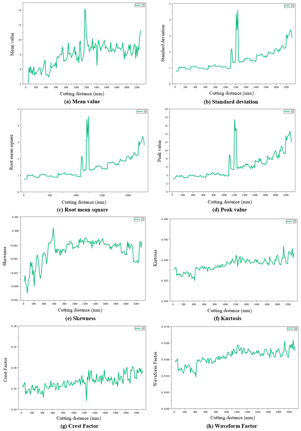
The time domain captures the original waveform of the signal as it evolves over time. Tool wear is a gradual process that can be directly reflected in the amplitude variation of the cutting signals. In this paper, eight time domain features, namely the mean, standard deviation, root mean square (RMS), peak value, skewness, kurtosis, crest factor, and waveform factor, were calculated to analyze the energy consumption and impact characteristics in the cutting signal induced by the tool wear process. These features, which are particularly sensitive to the severe tool wear stage of tool life, can be applied as intuitive wear severity indicators for the recognition model.

The calculated time domain features from the strain signal are illustrated in Figure 5. From the results, the time domain features of the strain signal evolve systematically with increasing cutting distance. The mean, standard deviation, RMS, and peak value all exhibit an overall upward trend with increasing cutting distance. They indicate a gradually increasing energy consumption in the cutting process. The skewness and kurtosis also increase, indicating growing asymmetry and impulsiveness in the signal distribution. Correspondingly, the crest factor and form factor rise, further confirming amplified impact components. These variations demonstrate that the extracted features in the time domain are sensitive to the gradual tool wear process and can serve as intuitive indicators for tool wear severity, especially for the severe wear stage.

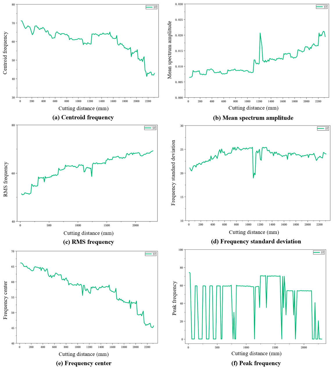
The sole time domain features in tool wear monitoring are insufficient. Feature extractions from additional domains were necessary to ensure the accuracy of tool wear monitoring. In this study, fast Fourier transform (FFT) was used to obtain the frequency domain features of the raw signal. Specifically, centroid frequency, mean amplitude, RMS frequency, standard deviation frequency, and peak frequency were extracted from the frequency spectrum to analyze their relationships with the tool wear process.

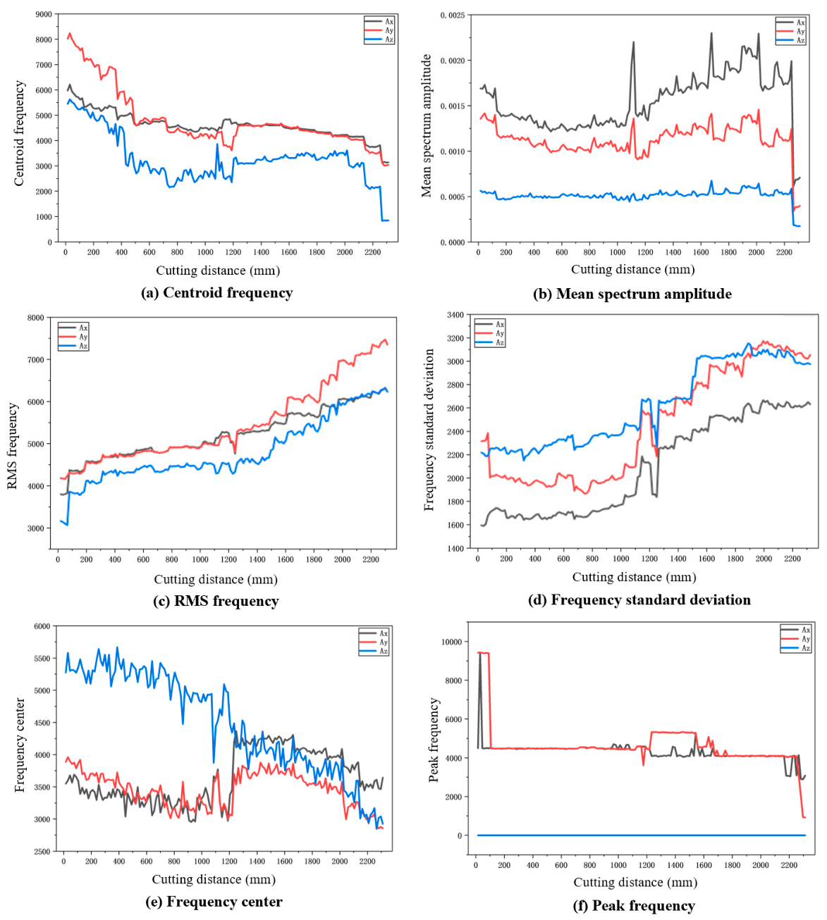
The calculated frequency features from the strain signal are shown in Figure 6. From the results, the frequency domain features of the strain signal exhibit pronounced trends with increasing cutting distance, revealing systematic spectral shifts driven by the tool wear process. Centroid frequency, frequency center, and peak frequency display an overall downward trend, indicating that spectral energy progressively concentrates toward lower frequency bands. Meanwhile, the mean spectrum amplitude, RMS, and standard deviation steadily rise, reflecting the intensified vibrational energy generated during the cutting process. Collectively, these frequency feature indicators also demonstrate clear sensitivity to the tool wear state, confirming the validity of frequency domain features for tool wear monitoring.

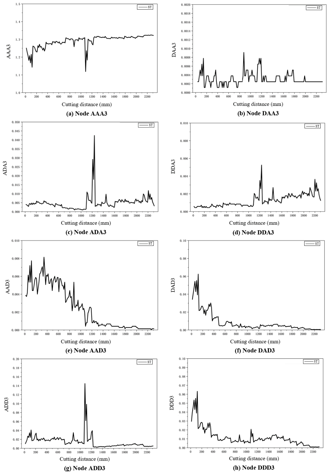
The tool wear process is complex and nonlinear and is further compounded by interference factors such as vibration and environmental noise. As a result, the acquired cutting signals are predominantly noisy and non-stationary, differing significantly from ideal stationary and continuous signals. Time domain and frequency domain analyses are inherently single-dimensional feature extraction methods; the features obtained can only reflect the local signal features in either the time or frequency domain. They are difficult to comprehensively capture the evolution of the tool wear process. Therefore, to enhance the accuracy of tool wear monitoring, time-frequency domain feature analysis must be performed on the cutting signals. Wavelet analysis can simultaneously acquire both time domain and frequency domain features and effectively captures the transient variations and non-stationary features of the cutting signal during the tool wear process. In this study, the db3 wavelet basis function was adopted to perform a three-level wavelet packet decomposition on the cutting signals.

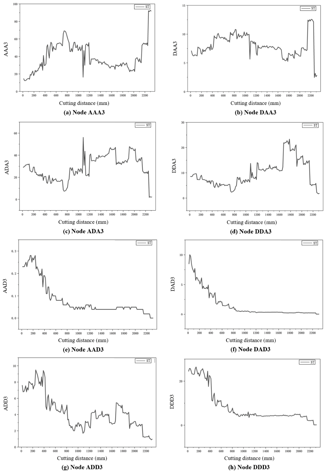
Figure 7 presents the wavelet packet decomposition results of the strain signal. From the results, the energy of the strain signal during the cutting process is predominantly concentrated in the low-frequency nodes, which represent spindle rotation and macroscopic loading. As the cutting distance increases and the tool dulls, the cutting force gradually rises, and the low-frequency nodes in the strain signal exhibit a steady upward trend throughout the tool life. Thus, they can serve as a core indicator for evaluating the tool wear process. In contrast, although the energy of mid- and high-frequency nodes such as the DAD3 and DDD3 decreases by orders of magnitude overall, they exhibit violent fluctuations in the initial wear stage. This accurately reflects the severe friction and micro-chipping that occurs in new tools in the running-in stage. Notably, at a cutting distance of approximately 1200 mm, the low-frequency nodes undergo a cliff-like drop, while synchronous sharp peaks appear in the mid- and high-frequency nodes such as ADA3 and ADD3. This pronounced inter-band energy transfer precisely captures an abrupt physical anomaly, which can be suspected to be local micro-chipping or impact with a hard phase in the workpiece material. Evidently, the temporal evolution of strain signals across different frequency bands comprehensively maps the physical progression of tool life from the initial running-in and normal wear stages to sudden failure. This demonstrates that the multi-band energy features extracted from the strain signal via wavelet packet decomposition are also effective in tool wear monitoring.

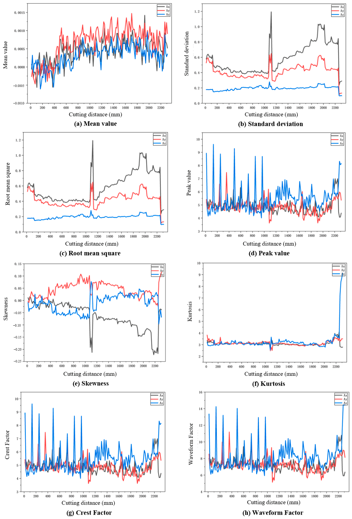
Figure 8 presents the calculated time domain features from the acceleration signals. From the results, the mean, standard deviation, RMS, and peak value of the acceleration signal exhibit a gradual increasing trend with cutting distance. They demonstrate a relatively high correlation with the tool wear process. This is because the increased tool wear value leads to a higher cutting force, which in turn intensifies vibration in the cutting system and consequently enhances the overall amplitude of the acceleration signal. The skewness of the acceleration signal is close to zero at the initial wear stage. With the tool wear process, skewness in the X and Z directions changes more notably, whereas skewness in the Y direction shows only minor variation. Kurtosis remains relatively small during the initial wear stage and increases significantly upon entering the severe wear stage, indicating the emergence of more impulsive components in the cutting process. The crest factor and form factor are relatively stable in the initial wear stage and rise somewhat in the severe wear stage, suggesting an increase in transient peak components and a weakening of periodicity in the cutting signal. Relatively, some features in the time domain exhibit a low correlation with the tool wear process and need to be eliminated through subsequent feature selection.

Figure 9 presents the frequency domain features of the acceleration signals. From the results, with the tool wear process, centroid frequency, frequency center, and peak frequency exhibit a decreasing trend with increasing tool wear, indicating a migration of signal energy toward the lower frequency band. This overall variation is consistent with that observed in the strain signal. With the tool wear process, the friction between the tool and the workpiece intensifies, which reduces system stiffness and increases the low-frequency vibration components. In the frequency domain, the mean amplitude, RMS, and standard deviation of the acceleration signal increase monotonically with tool wear, in agreement with the trends observed in the time domain.

Figure 10 presents the wavelet packet decomposition of the acceleration signals. Analysis of the signal amplitudes and energy distributions across the wavelet packet nodes reveals that during the initial wear stage, the high-frequency nodes such as DDD3 and ADD3 carry a relatively high proportion of energy, corresponding to high-frequency vibration components generated when the cutting edge of a new tool is sharp. With the tool wear process, the signal amplitudes at the low-frequency nodes such as AAA3 increase markedly, while energy at the high-frequency nodes gradually decreases. This also confirms energy migration toward lower frequencies. Meanwhile, some intermediate frequency nodes such as the DAA3 and ADA3 exhibit energy fluctuations in the middle and late stages of tool life.

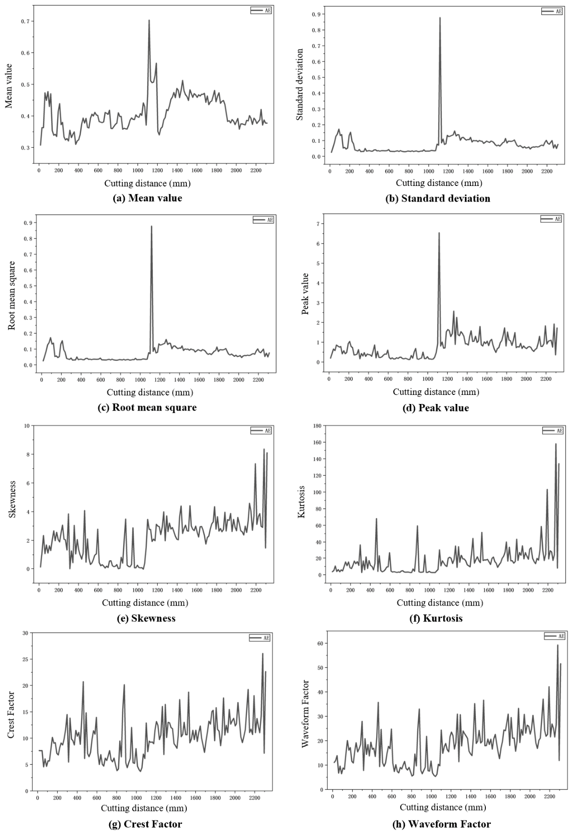
The time domain features calculated for the AE signal are presented in Figure 11. From the results, it can be observed that with increasing cutting distance, the time domain features of the AE signals exhibit trends that are highly correlated with the tool wear process. The mean value remains at a low level, which is consistent with the random fluctuation feature of the AE signals. The standard deviation, RMS, and peak value show a distinct upward trend with the tool wear process. They directly reflect the gradual increase in energy consumption by material plastic/elastic deformation and friction action in the cutting process, thereby demonstrating a strong correlation with the tool wear process. The skewness and kurtosis of the AE signals display pronounced nonlinear fluctuations. It indicates that the signal distribution gradually deviates from a normal distribution with the tool wear process, accompanied by an increasing number of impact components and abrupt features. The crest factor and form factor exhibit an overall upward trend, effectively characterizing the impact intensity and waveform distortion of the AE signals, and they respond well to the tool wear state.

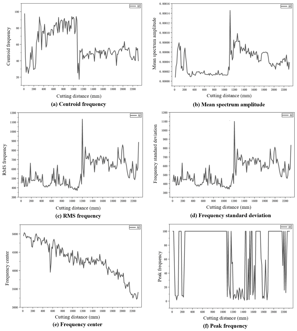
Figure 12 presents the frequency features calculated from the AE signals. Overall, with the tool wear process, the centroid frequency exhibits a gradually decreasing trend, indicating the migration of energy toward lower frequency bands. The mean amplitude increases with the tool wear process, which is consistent with the trend of the RMS value in the time domain. It further corroborates the conclusion that the tool wear process leads to an enhancement in signal energy. The standard deviation frequency remains relatively stable during the initial wear stage but undergoes a distinct shift upon entering the severe wear stage. It indicates that the shape and dispersion of the frequency distribution are reorganized during the severe wear stage. From these results, it can be inferred that some frequency domain features of the AE signal can effectively capture the dynamic variations in the cutting system caused by tool wear and can thus serve as effective indicators for tool wear monitoring.

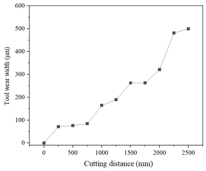
In this study, the tool wear experiments were repeated four times using four new cutting tools and workpieces. In the tool wear experiments of each tool, 160 sets of signal feature samples were extracted at equal cutting distance intervals. And a total of 640 sets of signal feature samples were extracted from the four used tools, which constitute the final feature dataset. These signal feature samples were divided into two parts: the training set which is composed of three tools, and the test set, which is composed of one tool. As shown in Figure 2, the tool wear process can be divided into three stages, namely the initial wear stage, the normal wear stage, and the severe wear stage. Then, the extracted feature dataset was labeled into three classes: the signal feature in the initial wear stage was labeled 0, the signal feature in the normal wear stage was labeled 1, and the severe wear stage was labeled 2. A total of 480 sets of the labeled training set are detailed in

Table 2. The tool wear signal feature data set.

NO	Peak Frequency of AE Signal	Peak Frequency of Strain Signal	Node DAA3 of Strain Signal	…	Mean Value of AE Signal in the X Direction	Label
1	7.62939	7.74326	0.15	...	0.00027	0
2	7.62939	7.74326	0.17	...	0.00005	0
3	7.62939	7.74326	0.17	...	0.00016	0
...	...	...	...	...	...	...
148	0.95367	6.83229	0.15	...	0.00043	2
149	1.43051	7.74326	0.19	...	0.00028	2
150	1.19209	0.91097	0.25	...	0.00022	2
...	...	...	...	...	...	...
237	6.91414	6719.78851	0.06	...	0.00073	1
238	8.58307	6678.33926	0.07	...	0.00080	1
239	7.86781	6696.78645	0.09	...	0.00063	1
...	...	...	...	...	...	...
478	12.87460	7.74326	0.08	...	0.00071	2
479	8.58306	15.48653	0.07	...	0.00113	2
480	17.16613	15.48653	0.07	...	0.00049	2

. This dataset is theoretically sufficient to verify the machine learning model, and more tool wear signal data can be further collected for model training to improve model robustness and generalization capability for industrial applications.

3.2. Feature Selection and Fusion for Tool Wear Monitoring

Through feature extraction of the strain, acceleration, and AE signals acquired during tool wear progression, a total of 102 sets of features were obtained. These signal features belonged to different physical quantities; they needed to be normalized before multi-signal fusion. Multi-signal fusion at the feature level established feature vectors, which were then used as input for the machine learning model to carry out the tool wear status prediction. Additionally, due to the excessive number of 102 feature signals, which affected computational efficiency, it was necessary to filter the feature signals to obtain the key features that are highly correlated with tool wear, thereby reducing the dimension of the feature vectors and improving model training efficiency.

Due to significant differences in the sensitivity of different signals to the tool wear process, as well as variations in tool quality and their initial installation states, there were non-stationarity and individual differences in the acquired signals. Hence, before signal feature normalization, according to the chronological order of the machining process, sliding window local normalization was performed on the established feature vectors to eliminate local scale differences. And an online cumulative self-calibration time correction method was also performed to correct the systematic offsets caused by temperature drift, operational condition changes, etc. This strategy can realize the adaptive drift compensation of the signal features. It converts the current feature values into drift-compensated feature values without introducing information from future samples, thereby providing more reliable feature inputs for the tool wear prediction model.

The acquired strain, acceleration, and AE signals in the tool wear experiments belong to different physical quantities. The strain signal is a mechanical, physical quantity; vibration is a kinematic, physical quantity; and the AE signal is an unmeasurable physical quantity. In feature normalization of multi-signals, the traditional Z-score normalization method is relatively dependent on the stability of data distribution. However, various abnormal situations often occur during the tool wear process. When abnormal values in monitoring signals are detected, it is prone to cause the problem of data scale deviation. Hence, the steady scaling method was applied to standardize the multi-signal features. The mean value was replaced by the median of each signal feature as the central position, and the standard deviation was replaced by the interquartile range as the scale measurement. The median value and the interquartile range belong to steady statistics and are not sensitive to abnormal situations. Therefore, in the presence of sensor noise interference or when the data distribution is skewed, this method exhibits greater stability. The calculation formula for signal feature normalization based on the steady scaling method is as follows:

$$x^{*}={\displaystyle \frac{x-{\mathrm{Q}}_{0.5}\left(\mathrm{X}\right)}{{\mathrm{Q}}_{0.75}\left(\mathrm{X}\right)-{\mathrm{Q}}_{0.25}\left(\mathrm{X}\right)}}$$

(3)

where $x^{*}$ represents the standardized value after normalization, X represents the set of feature samples, ${\mathrm{Q}}_{0.25}\left(\mathrm{X}\right)$, ${\mathrm{Q}}_{0.5}\left(\mathrm{X}\right)$, and ${\mathrm{Q}}_{0.75}\left(\mathrm{X}\right)$ respectively represent the lower quartile, median, and upper quartile of signal features, and ${\mathrm{Q}}_{0.75}\left(\mathrm{X}\right)-{\mathrm{Q}}_{0.25}\left(\mathrm{X}\right)$ represents the interquartile range. In this work, the signal feature dataset in Table 2 was divided into the training set and test set with a fixed proportion, and the steady scaling method was conducted for the training set. Through this signal feature normalization method, the scale bias problems caused by missing features, abnormal value, and dimensional differences can be effectively alleviated. It can provide more reliable normalized input features for the tool wear prediction model.

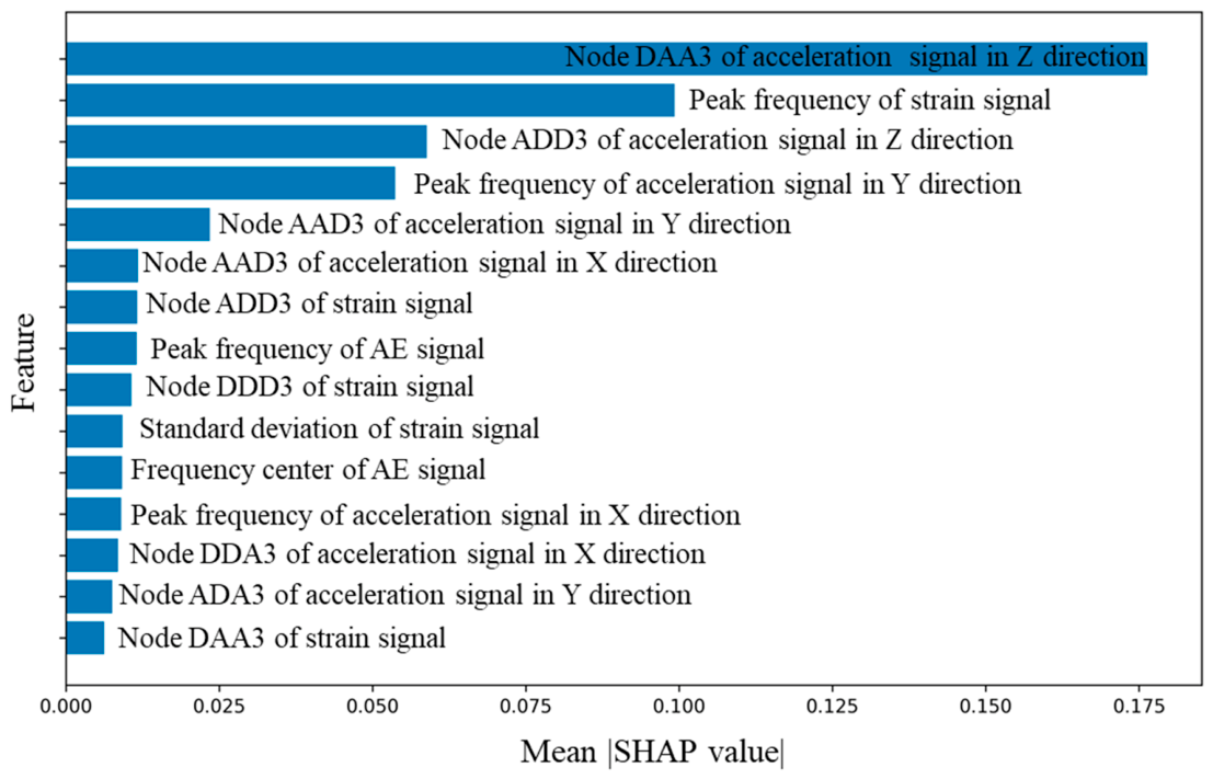
Subsequently, the minimum redundancy and maximum relevance (mRMR) feature selection method was used to select signal features. The candidate signal features were subjected to deduplication and denoising, then ranked in decreasing order by their importance scores. Adaptive selection was subsequently performed through a K-value constraint, selecting a low-redundancy, high-sensitivity optimal feature subset that can serve as input for the subsequent tool wear monitoring model. In feature selection by mRMR, Shapley Additive Explanations (SHAP) values were further used to assess the importance of each feature’s contribution to the tool wear prediction model. Finally, the 15 most important features with the highest contribution scores to the tool wear prediction model were selected, as shown in Figure 13. It can be observed that these features already comprehensively capture the main multi-signal information closely related to tool wear prediction. This feature subset helps reduce the computational burden and overfitting risk associated with redundant features and provides a direct basis for determining the input features of the subsequent model.

Based on classification statistics for these selected features, it was found that two features belong to the AE signal, five belong to the strain signal, and eight belong to the acceleration signals. They cover all sensors and can achieve complementary multi-information fusion. With respect to feature type, one is a time domain feature, five are frequency domain features, and nine are time-frequency domain features. This distribution indicates that the tool wear process is a typical non-stationary dynamic process. The time-frequency domain features, which can simultaneously capture instantaneous signal variation and frequency distribution patterns, possess a stronger characterization capability for tool wear progression than the time domain features. This result is consistent with the non-stationary nature of the force, vibration, and AE signals induced by the tool wear process in actual machining. These selected key features were used to construct the feature vectors for multi-signal fusion, which serve as the input for the tool wear monitoring model.

3.3. Tool Wear Monitoring Based on an Integrated Model

The commonly used machine learning models struggle to balance accuracy with generalization in tool wear monitoring based on multi-signal feature fusion due to nonlinear coupling, distribution discrepancies, and noise interference. To address these issues, a weighted integrated model is proposed in this paper. Six classical machine learning models that are suitable for tool wear monitoring were compared, and the models that can adapt to multi-signal feature fusion and possess excellent generalization performance were selected to establish the weighted integrated model. The six classical machine learning models are as follows:

(1) Ridge regression model. It is an improved version of linear regression that incorporates an L₂ regularization term. The objective function is expressed as follows:

$$L\left(B\right)={\displaystyle \sum _{i=1}^N}{\left(y_i-x_i^T\beta \right)}^2+\alpha {‖\beta ‖}_2^2$$

(4)

where $y_i$ represents the true flank wear value VB of the i-th sample, the second term is the L₂ regularization term, and α is the regularization strength coefficient.

(2) K-nearest neighbors regression model (KNN). The KNN model is a typical non-parametric machine learning approach. It does not require a pre-specified explicit functional form and performs regression prediction by leveraging local sample information. The model is expressed as follows:

$${\widehat{y}}_q={\displaystyle \frac{1}{k}}\sum _{i\in N_k\left(x_q\right)}{y}_i$$

(5)

where ${\widehat{y}}_q$ is the predicted tool wear value for the query sample $x_q$, $N_k\left(x_q\right)$ denotes the set of k-nearest neighbors of the query sample $x_q$, and $y_i$ is the target value of the i-th sample within this neighbor set.

(3) Random forest model. This model is a classic learning model based on the Bagging integrated strategy. It can independently construct multiple decision trees and average their outputs, thereby significantly reducing the prediction variance of an individual decision tree. This effectively improves the overall stability and generalization capability of the model. The model is expressed as follows:

$$\widehat{y}={\displaystyle \frac{1}{B}}{\displaystyle \sum _B^1}{T}_b\left(x\right)$$

(6)

where $\widehat{y}$ is the predicted tool wear value, B is the number of decision trees, and $T_b\left(x\right)$ is the output of the b-th decision tree.

(4) Extreme random tree model (extra trees). It is an improved learning method developed from the random forest model. It can reduce correlation among base learners by introducing greater randomness, thereby optimizing ensemble performance. The final prediction output of this model is the ensemble average of the predictions from all decision trees. The model is expressed as follows:

$$\widehat{y}={\displaystyle \frac{1}{B}}{\displaystyle \sum _{b=1}^B}{T}_b^{test}\left(x\right)$$

(7)

where B is the number of decision trees, and $T_b^{test}\left(x\right)$ represents the prediction output of the b-th tree.

(5) Histogram-based gradient boosting regression model (HistGBR). This model is an engineering implementation of the gradient boosting decision tree (GBDT) model. By applying histogram binning to continuous features, it discretizes feature values into a finite number of intervals to substantially reduce the computational cost of node splitting and significantly improve model training efficiency. The model is expressed as follows:

$$f\left(x\right)={\displaystyle \sum _{m=1}^M}c{h}_m\left(x\right)$$

(8)

where $h_m\left(x\right)$ is the m-th regression tree, and c is the learning rate that governs the update magnitude of each individual tree on the overall model.

(6) TabPFN regression model. This model is a foundational model based on Transformer architecture that is specifically designed for tabular data. By pre-training on large-scale synthetic data tasks, it acquires the capability of rapid adaptation to unseen tasks. The model is expressed as follows:

$$\widehat{y}=f_{PEN}\left(x|D_{train}\right)$$

(9)

where $D_{train}$ denotes the set of training samples.

A progressive modeling strategy was adopted to establish the weighted integrated model in this study; detailed steps include within-group cross-validation, model selection, and weighted ensemble. Through within-group cross-validation, base models with high prediction accuracy and complementary outputs were selected from six candidate models, and the integrated model was subsequently constructed by the weighted method to enhance the overall accuracy and stability of tool wear prediction.

According to the tool wear standard and the tool wear experiment results in Figure 2, thresholds based on the flank wear width VB for the three tool wear stages were defined: initial wear with flank wear width VB is less than 0.1 mm, normal wear with flank wear width VB is 0.1–0.3 mm, and severe wear with flank wear width VB is larger than 0.3 mm, as follows:

$$\mathrm{Tool} \mathrm{wear} \mathrm{state} \left\{\begin{array}{c}\mathrm{I}\mathrm{n}\mathrm{i}\mathrm{t}\mathrm{i}\mathrm{a}\mathrm{l} \mathrm{w}\mathrm{e}\mathrm{a}\mathrm{r} \mathrm{s}\mathrm{t}\mathrm{a}\mathrm{g}\mathrm{e}, VB<100 \mathsf{\mu }\mathrm{m}\\ \mathrm{N}\mathrm{o}\mathrm{r}\mathrm{m}\mathrm{a}\mathrm{l} \mathrm{w}\mathrm{e}\mathrm{a}\mathrm{r} \mathrm{s}\mathrm{t}\mathrm{a}\mathrm{g}\mathrm{e}, 100<VB<300 \mathsf{\mu }\mathrm{m}\\ \mathrm{S}\mathrm{e}\mathrm{v}\mathrm{e}\mathrm{r}\mathrm{e} \mathrm{w}\mathrm{e}\mathrm{a}\mathrm{r} \mathrm{s}\mathrm{t}\mathrm{a}\mathrm{g}\mathrm{e}, VB\ge 300 \mathsf{\mu }\mathrm{m}\end{array}\right.$$

(10)

Firstly, 480 multi-signal feature samples from the training set presented in Table 2 were preprocessed. Then, candidate model training and evaluation were carried out using five-fold within-group cross-validation. Based on the tool wear prediction values output by the candidate model, tool wear state was determined according to the aforementioned threshold in Equation (10).

In this work, regression algorithms were first adopted to predict the continuous tool wear value and then realize wear state classification based on the predicted results. And then the average value of root mean square error (RMSE) was used to quantitatively assess the performance of extra trees, random forest, and ridge regression in base model selection, which is a widely used regression evaluation metric and can be calculated by the following equation:

$$RMSE=\sqrt{{\displaystyle \frac{1}{N}}{\displaystyle \sum _{i=1}^N}{\left(y_i-{\widehat{y}}_i\right)}^2}$$

(11)

where $y_i$ represents the measured tool wear value, and ${\widehat{y}}_i$ represents the predicted tool wear value by the model.

Table 3. RMSE results of candidate models.

No	Candidate Model	RMSE
1	Extra trees	234.309791
2	Ridge regression	238.651449
3	Random forest	239.433112
4	TabPFN	241.377299
5	HisGBR	245.527223
6	KNN	318.634271

presents the calculated RMSE results of the six candidate models. The smaller the RMSE is, the smaller the regression prediction error of the model for the actual tool wear will be, and thus the better the prediction performance and generalization ability of the model will be. From the results, the RMSE of the extreme random tree model, ridge regression model, and random forest model are relatively smaller than those of other models. Therefore, these three models were selected as the base model for further model integration because they exhibit strong complementarity. The extreme random tree model introduces a stronger randomization mechanism, thus offering superior generalization ability. The ridge regression model is capable of stably extracting the overall linear trend of tool wear evolution under conditions of high-dimensional and strongly correlated features. By contrast, the random forest model provides higher stability and greater robustness against noise. Moreover, both the extreme random tree model and random forest model can effectively characterize the complex nonlinear relationships and high-order interactions between multi-signal features and the tool wear process.

In model integration, the selected models were normalized and weighted based on the reciprocal of the square of the RMSE results. This method can allocate integration weights based on the prediction errors of each model on the validation set and can ensure the model with smaller prediction errors will obtain a greater weight in the final integrated model. It means that the smaller the prediction error, the greater the candidate model weight. The candidate model weight can be expressed as:

$$w_m={\displaystyle \frac{1/{RMSE}_m^2}{{\sum }_{j=1}^M{1/RMSE}_j^2}}$$

(12)

where $w_m$ represents the weight for the m-th candidate model, ${RMSE}_m$ represents the RMSE result for the m-th candidate model, and M represents the total number of candidate models.

Based on this method, the calculated weight values are respectively 0.3423, 0.3299, and 0.3278 for the extreme random tree model, ridge regression model, and random forest model. The output of the final integrated model is the weighted sum of the prediction results from each model, as shown in the following equation:

$$\widehat{y}={\displaystyle \sum _{m=1}^M}{w}_m{\widehat{y}}_m$$

(13)

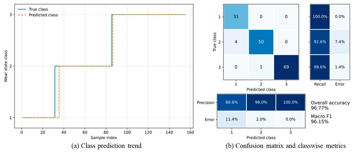
After calculating the weights of the integrated model, 160 sets of signal feature samples from the test set not involved in the model training were introduced into the integrated model to predict the corresponding tool wear state classification. The tool wear prediction classification results on the tool wear dataset of the test set are presented in Figure 14. The results indicate that the integrated model did not make any misjudgments in the initial wear stage, with an identification accuracy rate of 100%. In the normal wear stage, a total of four samples were misjudged, with an accuracy rate of 92.6%, and in the severe wear stage, only one sample was identified incorrectly, with an accuracy rate of 98.6%. Overall, the comprehensive identification accuracy of the integrated model reached 96.77%. This verifies the effectiveness and reliability of the proposed integrated model for tool wear monitoring.

As shown in

Table 4. Prediction accuracy rate of candidate models.

No	Model	Prediction Accuracy Rate
1	Integrated model	96.77%
2	Extra Trees	88.39%
3	Ridge Regression	88.06%
4	Random Forest	68.39%

, a comparison of prediction accuracy rates between the integrated model and single models on the test set is presented. From the results, the comprehensive prediction accuracy rates of the three single models were 88.39%, 88.06%, and 68.39%, respectively. After the weighted integration of the three single models, the prediction accuracy rate increased to 96.77%, which is significantly higher than the accuracy rate of the single models, indicating that the integrated model can more accurately identify tool wear states compared with the single model.

4. Conclusions

In this paper, a study on tool wear monitoring by multi-signal fusion based on an integrated machine learning model is conducted. From the results, the following conclusions can be drawn:

• Different signals are compared, and surface strain, acceleration, and AE signals are selected as tool wear monitoring signals based on distinct types of physical quantities and installation convenience. Then, synchronous multi-signal acquisition is carried out through tool wear experiments. After signal denoising, a feature set including time domain, frequency domain, and wavelet packet time-frequency domain features is constructed, from which a total of 102 features are extracted.
• The mRMR method is employed to select the key features from the 102 extracted features, and 15 key features that are highly correlated with the tool wear process while exhibiting low redundancy are selected. By this method, feature dimensionality is reduced from 102 to 15. These selected key features are used to construct the feature vectors for multi-signal fusion, which serve as input for the tool wear monitoring model.
• An integrated model is proposed for tool wear monitoring. By comparing six typical machine learning models, three complementary models, namely the extreme random tree model, ridge regression model, and random forest model, are selected to construct the integrated prediction model. The results indicate that the integrated model obtains an overall tool wear state classification accuracy of 96.77%. The results confirm the effectiveness and reliability of the proposed integrated model.