Active Suspension Performance Modeling: Domain Shift and Road-Class Transferability Across ISO 8608 Road Profiles

Abstract

Data-driven active-suspension models are often judged by aggregate prediction accuracy. For road-adaptive control and diagnostics, however, a model is useful only if its predictions remain reliable when road severity changes. This study asks how far an active-suspension response model trained under one set of ISO 8608 road classes can be transferred to another. A Quanser-based benchmark dataset containing ISO classes A–E is used to evaluate predictability, explainability, and transferability in the same workflow. Sample-level body and tyre displacement models are tested with leave-one-road-class-out validation, while window-level body/tyre RMS and peak indicators are tested through adjacent, graded, and A–D to E transfer scenarios. Transfer loss is quantified with a relative transferability ratio (RTR), defined as the ratio between transfer $R^2$ and in-domain $R^2$. Sample-level tyre displacement transfers more consistently than body displacement, with RTR values of 0.887–0.984 for tyre response and 0.376–0.982 for body response. By contrast, window-level transfer to class E fails for body RMS and peak response and remains weak for tyre RMS, showing that accurate displacement reconstruction does not necessarily translate into transferable engineering indicators. PCA centroid and Wasserstein distances are strongly negatively correlated with RMS RTR, linking transfer degradation to road-feature domain shift. Frequency-band analysis shows that class E produces disproportionate body and tyre response-energy increases in selected low- and mid-frequency bands. SHAP analysis indicates that road RMS dominates tyre–RMS transfer, whereas body–RMS transfer depends mainly on road peak and road RMS. A secondary SOF-controlled dataset is kept separate as a control-effort consistency check. The resulting contribution is an interpretable predictability–explainability–transferability assessment for active-suspension benchmark data, not a new controller, road classifier, or system-identification method.

1. Introduction

Vehicle suspension systems must attenuate road-induced vibration while maintaining tyre-road contact and keeping suspension travel and actuator demand within acceptable limits. These requirements are coupled rather than independent, so ride comfort, road holding, suspension working space, and control effort are normally assessed together [1,2]. Switching and mode-dependent formulations also show that the balance among these objectives changes with operating condition [3]. Active suspension systems enlarge the design space by adding controlled actuation between the sprung and unsprung masses, but this benefit also makes performance more dependent on the road domain in which the controller or model is evaluated.

The active-suspension literature reflects this breadth of objectives. Robust and sliding-mode methods remain central to controller design [4,5]. Finite-time control and explicit MPC formulations address convergence, constraints, and operating-region dependence [6,7]. Preview MPC uses road information before the disturbance reaches the suspension, while fuzzy-LQR designs embed rule-based or optimal-control structure in the controller [8,9]. FLQG/LQG designs extend the same idea through fuzzy and linear-quadratic control concepts [10]. Data-driven control co-design has also been studied through reinforcement learning and digital-twin concepts [11]. Recent work further covers time-delay compensation and static-output-feedback implementation [12,13]. Safety constraints and fixed-time fuzzy control have also been treated explicitly [14,15]. Reinforcement-learning studies on active and semi-active suspensions point to growing interest in adaptation under changing conditions [16,17]. Experimental work gives the same question a practical grounding: quarter-car and passivity-based studies show that implementation conditions matter when judging performance [18,19]. Hydraulic and double-wishbone active-suspension experiments provide complementary implementation contexts [20,21].

These research directions answer related but different questions. Controller-oriented studies mainly ask whether a selected controller improves closed-loop response under prescribed disturbances. Road-classification and identification studies ask whether the road class or the input–output dynamics can be inferred from measured signals. Data-driven diagnostics raise a more specific reliability question: if a response model is trained under one road-severity domain, how much of its predictive value remains when it is deployed under another road class?

The present study addresses this gap using two independent Quanser-based active suspension datasets. The first dataset is the Mendeley Data record associated with robust ${\mathcal{H}}_{\infty }$ control with $\mathcal{D}$-stability via static output feedback (SOF) for nonlinear active suspension systems [22]. It includes road displacement, sprung-mass displacement, unsprung-mass displacement, system states, and control force during open-loop and closed-loop experimental intervals. The corresponding controller study provides the SOF design context [23]. The second dataset is the Zenodo benchmark vehicle-suspension dataset based on ISO 8608 road profiles [24]. Related Quanser suspension measurements have previously been used for road classification and resonant-system identification [25,26]. The road-class terminology follows the ISO 8608 road-profile reporting standard [27].

This paper concentrates on joint predictability, explainability, and transferability assessment rather than on a new controller or road-classification algorithm. The ISO 8608 dataset forms the core of the study because it permits controlled leave-one-road-class-out and A–D to E transfer tests. The SOF-controlled dataset is retained only as a secondary control-effort consistency check.

The main contributions are:

• A leave-one-road-class-out evaluation of sample-level body and tyre displacement transfer across ISO 8608 classes A–E.
• A relative transferability ratio comparing cross-class transfer accuracy with in-domain prediction accuracy.
• Adjacent, graded, and broad window-level performance-index transfer tests across ISO road classes.
• Domain-distance, SHAP, PCA, and frequency-band analyses linking transfer degradation to road-feature shift.
• A secondary SOF control-effort consistency check, kept separate from the ISO transferability claims.

2. Related Work

Robust SOF control for nonlinear active suspension systems has been studied with Takagi–Sugeno fuzzy modeling, $\mathcal{D}$-stability constraints, and ${\mathcal{H}}_{\infty }$ disturbance attenuation [23]. Static-output-feedback designs are particularly relevant when full-state measurement is unavailable or undesirable in implementation [13]. Broader robust and nonlinear control studies have treated actuator faults and input quantization [4,28]. Time-delay actuation and adaptive finite-time convergence form a parallel concern [12,29]. Constraints on displacement, safety, and convergence have also been addressed through fixed-time fuzzy and sliding-mode formulations [14,15]. Together, these studies establish controller feasibility under uncertainty and implementation limits. Their evaluations, however, are usually organized around prescribed disturbances, model uncertainty, actuator behavior, or experimental validation; they do not directly measure whether a learned response or performance-index model remains reliable when it is moved from one ISO road-class domain to another.

Optimal, preview, fuzzy, and data-driven control studies provide a second line of context. Regionless explicit MPC and road-preview MPC have been used to reduce body acceleration and exploit previewed road information [7,8]. ANN-based semi-active suspension and fuzzy-LQR designs show how learning or rule-based elements can be embedded in suspension control architectures [9,30]. FLQG/LQG designs extend this direction by combining fuzzy logic with linear-quadratic control concepts [10]. Road-recognition-based fuzzy PID control connects estimated road information directly to controller adaptation [31], and adaptive neuro-fuzzy active-suspension control has likewise been used to switch performance-oriented control behavior across road-profile conditions [32]. Linear-quadratic finite-state control and magnetorheological-damper adaptive control both treat changes in operating condition as central to performance assessment [33,34]. Adaptive optimal semi-active control gives the same role to exogenous road disturbance [35]. Reinforcement-learning studies make the point from a data-driven perspective, including online actor-critic and PPO formulations [36,37]. Deep reinforcement learning and ISO-comfort-oriented reinforcement learning provide further examples [16,17]. Digital-twin-enabled reinforcement-learning co-design extends this trend to full-vehicle active suspension systems [11]. Experimental studies also keep the evaluation problem grounded in implementation: quarter-car and passivity-based experiments show that controller behavior should be judged under practical constraints as well as in simulation [18,19]. Active hydraulic and double-wishbone suspension experiments provide complementary validation contexts [20,21].

The ISO 8608 benchmark dataset has been used for two distinct purposes. Tan et al. [25] proposed a built-in self-scaling Bayesian regression method for ISO road-class classification using frequency-response magnitude patterns, showing strong classification performance under passive and active suspension conditions. Road excitation and roughness recognition studies similarly show that measurable suspension or tyre responses can support road classification for adaptive suspension use, including deep-neural-network classification from sprung and unsprung responses and intelligent-tyre-based road classification for real-time semi-active control [38,39,40]. Tan and Foo [26] later used related Quanser suspension measurements for kernel design in resonant-system impulse-response estimation, showing that incremental Kautz-kernel designs can capture multiple resonances in experimental data.

These studies establish the value of the available data, but they also define the remaining gap. Road-recognition and adaptive-control methods use road information to improve or tune suspension behavior [31,32,36]. PPO and deep reinforcement-learning studies likewise exploit data-driven adaptation for suspension control [16,37]. Other reinforcement-learning work evaluates active-suspension control with comfort-oriented criteria [17]. In a related pavement-monitoring context, transfer learning has been used to reconcile vehicle-response data with standard roughness indices, with generalization reported to depend on the coverage of rougher road profiles [41]. What remains less explicit is the degradation of a learned response or performance-index model when the target road class is outside the training domain. The present study does not repeat ISO road classification, built-in self-scaling Bayesian regression, road-roughness recognition, Hammerstein–Wiener identification, subspace identification, or Kautz-kernel impulse-response estimation. It reframes the benchmark from classification or identification toward model reliability under road-severity shift.

3. Materials and Methods

3.1. Dataset Description

Two datasets are used. Dataset 1 is the robust SOF active-suspension dataset archived on Mendeley Data by Yamanaka et al. [22]. It contains 40,001 samples at a sampling interval of $0.0010$ s. The main variables are road displacement $z_r$, sprung-mass displacement $z_s$, unsprung-mass displacement $z_{us}$, control force $F_c$, and state variables. The original experiment contains an open-loop interval from 0 to 6.0000 s, after which the SOF controller is activated. This dataset is methodologically aligned with SOF active-suspension work, where measured outputs rather than full-state feedback are used for controller realization [13,23]. The platform context is consistent with the Quanser laboratory-scale active-suspension system documentation (Quanser Inc., Markham, ON, Canada) [42].

Dataset 2 is the ISO 8608 benchmark dataset archived on Zenodo by Foo and Tan [24]. It contains road profiles for classes A–E, with non-harmonic-suppressed and harmonic-suppressed variants. Together with Dataset 1, its acquisition characteristics and analytical role are summarized in

Table 1. Summary of the two datasets considered in this study.

Property	Dataset 1: SOF Experiment	Dataset 2: ISO 8608 Benchmark
Platform family	Quanser active suspension	Quanser active suspension
Main excitation	Square-wave road input	ISO 8608 multisine road classes A–E
Samples	40,001	100,000 input; 400,000 response
Sampling interval	$0.0010$ s	$0.0010$ s
Recorded responses	$z_r$, $z_s$, $z_{us}$, $F_c$, states	Road, body displacement, tyre displacement
Control information	Available through SOF gain and measured $F_c$	Control-force signal not available
Primary role in this study	Secondary control-effort check	Primary transferability analysis

. The experimental system belongs to the same Quanser laboratory-scale vehicle-suspension platform family and is commonly represented as a resonant quarter-car suspension with road displacement input and body/tyre displacement outputs [26,42]. The road inputs contain 100,000 samples, and the corresponding body and tyre displacement responses contain 400,000 samples because the input period is repeated four times during measurement. Dataset 2 does not include control-force measurements, which is why it is used for road-class transferability rather than control-effort reconstruction.

3.2. Performance Indicators

The following indicators are computed where the required signals are available:

$$\begin{array}{cc}\hfill \mathrm{RMS}\left(x\right)& =\sqrt{{\displaystyle \frac{1}{N}}\sum _{k=1}^N{x}_k^2},\hfill \end{array}$$

(1)

$$\begin{array}{cc}\hfill x_{\mathrm{peak}}& =\underset{k}{max}\left|x_k\right|,\hfill \end{array}$$

(2)

$$\begin{array}{cc}\hfill z_{\mathrm{sws}}& =z_s-z_{us},\hfill \end{array}$$

(3)

$$\begin{array}{cc}\hfill z_{\mathrm{tire}}& =z_{us}-z_r,\hfill \end{array}$$

(4)

$$\begin{array}{cc}\hfill J_F& ={\int }_{t_1}^{t_2}{F}_c^2\left(t\right)dt.\hfill \end{array}$$

(5)

Ride comfort is evaluated using the sprung-mass response and, where appropriate filtering is applied, approximate sprung-mass acceleration. Road holding is evaluated using unsprung-mass response and tyre-deflection proxy $z_{us}-z_r$. Suspension working space is evaluated using $z_s-z_{us}$. These indicators are consistent with the comfort, handling, suspension-travel, and actuator-effort criteria commonly used in active-suspension performance assessment [1,2]. Experimental studies use related criteria when assessing active-suspension behavior under practical implementation constraints [18,19]. SOF and learning-based suspension studies also use comparable response and effort measures when evaluating controller performance [13,16]. Control effort is evaluated only for Dataset 1 because Dataset 2 does not include $F_c$.

3.3. Transferability Assessment

The data-driven layer is intended to assess model reliability, not to classify road profiles. The core analysis is performed on Dataset 2. For sample-level transfer, road displacement is used to predict body or tyre displacement from lagged road features. Extra Trees regression is used for these sample-level models because it can represent nonlinear lagged input–output relationships without requiring a parametric suspension model. Each target is evaluated with a leave-one-road-class-out protocol: four ISO road classes are used for training, and the remaining class is held out for testing. This split asks whether a model trained in one road-severity domain keeps its explanatory power in another.

For window-level transfer, one-second road windows are summarized by road RMS, peak value, standard deviation, peak-to-peak value, and band-power features. These features are then used to predict body/tyre RMS and peak indicators using Random Forest regression. The same model family is used for the adjacent, graded, and broad-transfer scenarios so that changes in RTR reflect road-domain transfer difficulty rather than a change in model architecture. The broadest transfer test trains on ISO classes A–D and tests on class E, the roughest road class in the dataset. This setting is more demanding than sample-level displacement prediction because RMS and peak indicators are closer to the quantities used in suspension design and monitoring.

Relative transferability is quantified using

$$\mathrm{RTR}={\displaystyle \frac{R_{\mathrm{transfer}}^2}{R_{\mathrm{in}-\mathrm{domain}}^2}},$$

(6)

where $R_{\mathrm{transfer}}^2$ is the score obtained on an unseen road class and $R_{\mathrm{in}-\mathrm{domain}}^2$ is the score obtained when training and testing within the same road class using a blocked split. Values close to 1 indicate that cross-class deployment approaches in-domain performance. Values near zero or negative indicate weak or failed transfer. Negative values are retained rather than clipped because they indicate transfer performance below a mean-prediction baseline. When the in-domain $R^2$ of the target class is non-positive, RTR is not reported, because the denominator no longer represents a meaningful positive reference performance.

Explainability is assessed using SHAP values for the window-level transfer models from classes A–D to class E. PCA maps the road-feature domain and provides centroid distances between training and target road domains. Mahalanobis distance and mean one-dimensional Wasserstein distance are also computed in the standardized road-feature space. These distances are correlated with RTR across adjacent and graded transfer scenarios to test whether poorer transfer is associated with measurable domain shift. Two-sided p-values are reported for Pearson and Spearman correlations, and paired bootstrap resampling with 10,000 resamples is used to estimate the 95% confidence interval of Pearson’s r. UMAP was not used, because PCA is deterministic, directly interpretable, and sufficient for the low-dimensional engineered feature set used here.

For Dataset 1, the target is the measured control force $F_c$, and the predictors are current and delayed values of $z_r$, $z_s$, $z_{us}$, $z_s-z_{us}$, and $z_{us}-z_r$. This SOF analysis is treated as a secondary consistency check because the measured control force is expected to be strongly reconstructable from measured outputs under a static-output-feedback control law [13,23].

3.4. Evaluation Strategy

The two datasets are not treated as interchangeable records. They differ in excitation type, protocol length, available variables, and control information. For that reason, the comparison is made at the level of normalized indicators and response-prediction behavior, rather than by merging all samples into a single training set.

The evaluation proceeds through:

• Computing ISO response scaling across road classes A–E;
• Evaluating sample-level leave-one-road-class-out prediction;
• Computing the relative transferability ratio for body and tyre displacement;
• Evaluating adjacent, graded, and A–D to E window-level transfer scenarios;
• Relating domain-distance metrics to RTR;
• Explaining transfer models with SHAP and visualizing road-feature domains with PCA;
• Computing frequency-band energy shifts across road, body, and tyre signals;
• Reporting SOF control-effort reconstruction as a secondary consistency check.

All numerical analyses were performed with Python 3.14.5. The analysis scripts used NumPy 2.4.6, pandas 3.0.3, SciPy 1.17.1, scikit-learn 1.8.0, Matplotlib 3.10.9, and SHAP 0.52.0. SciPy was used for reading MATLAB data files and signal processing, scikit-learn for Extra Trees regression, Random Forest regression, PCA, standardization, and performance metrics, Matplotlib for figure generation, and SHAP for tree-model explainability.

4. Results and Discussion

4.1. Road-Class Response Scaling

The ISO 8608 benchmark dataset provides a broader road-severity range than the SOF square-wave experiment.

Table 2. ISO 8608 non-suppressed road-class response indicators computed over the first steady-state response period.

Class	Road RMS [m]	Body RMS [m]	Tyre RMS [m]	Body/Road	Tyre/Road
A	0.000317	0.000490	0.000234	1.546	0.740
B	0.000573	0.000701	0.000488	1.224	0.852
C	0.001035	0.000752	0.000864	0.726	0.835
D	0.001871	0.001781	0.001711	0.952	0.914
E	0.003383	0.003584	0.003361	1.059	0.993

reports the non-harmonic-suppressed road profiles, which are sufficient to show the main response-scaling trend. The harmonic-suppressed variant was retained in the analysis files but is omitted here to keep the manuscript focused.

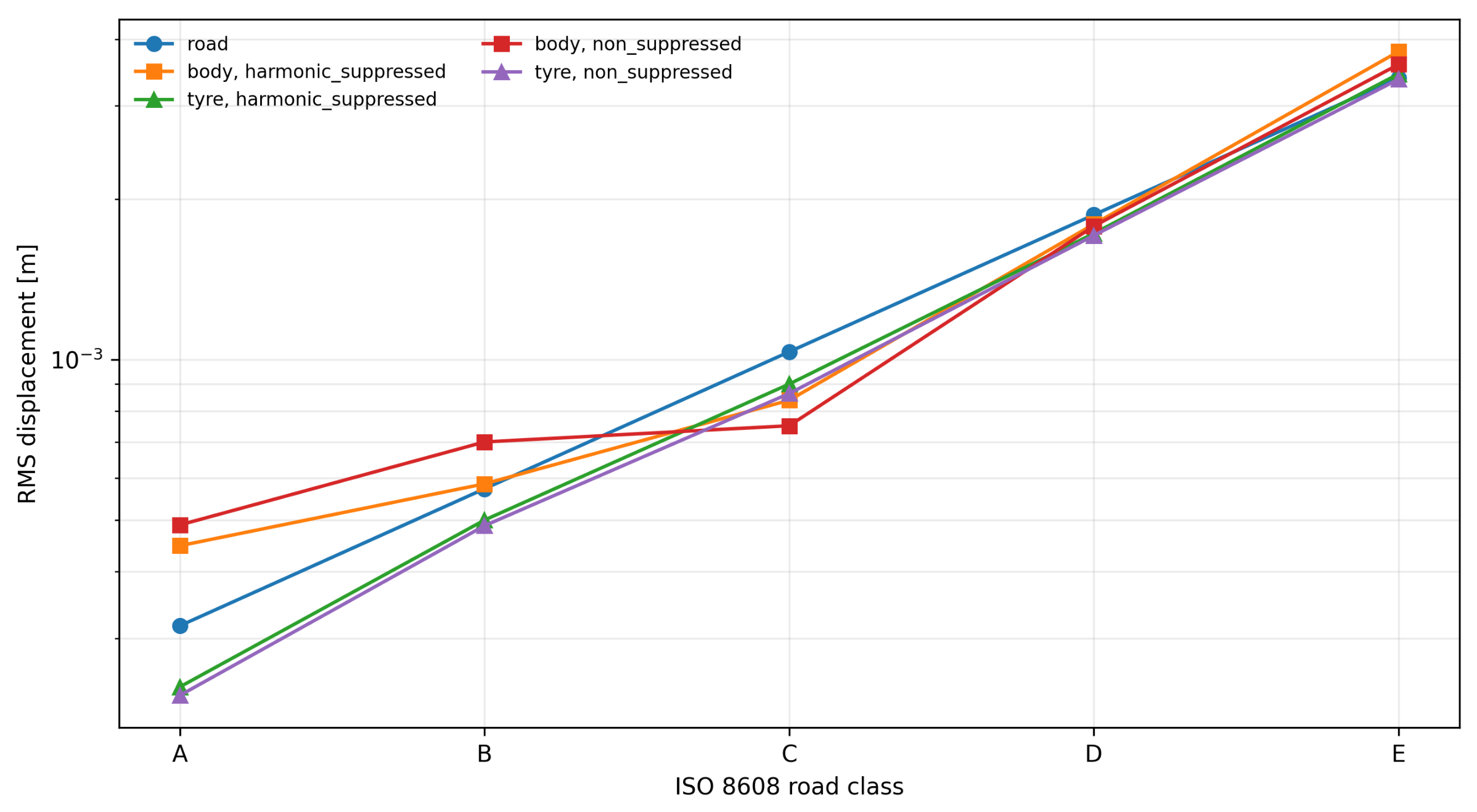
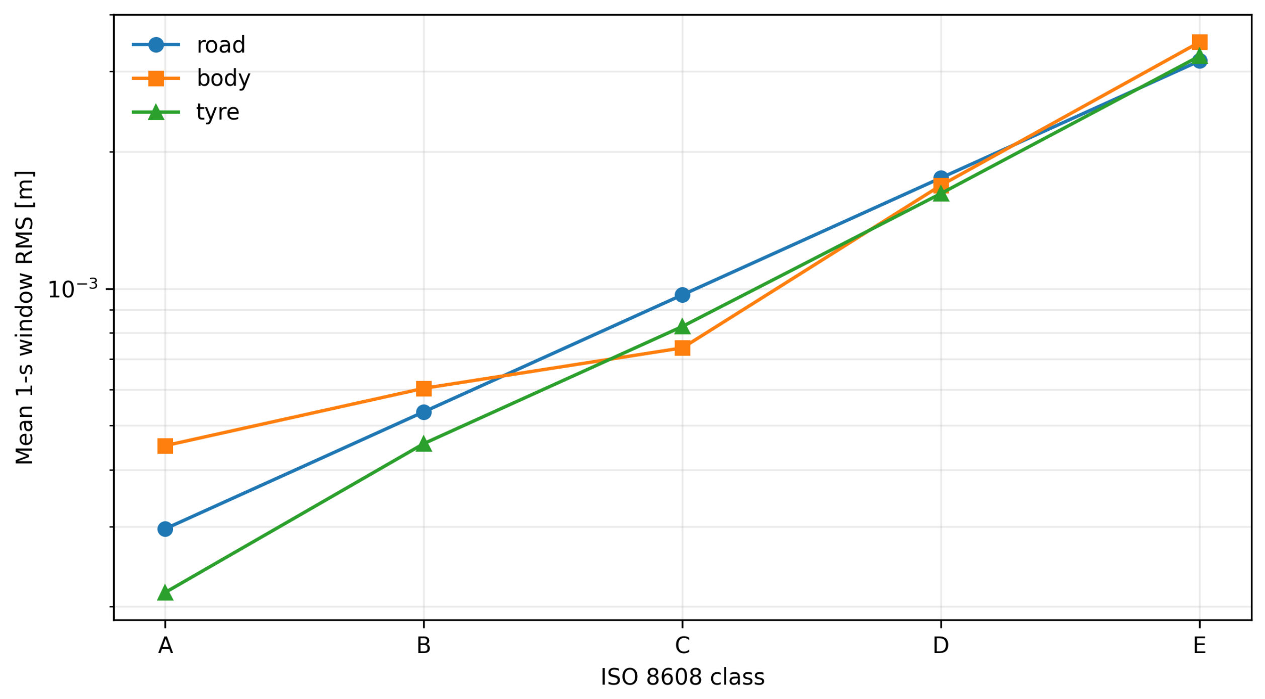
The same road, body, and tyre RMS progression is shown graphically in Figure 1, which makes the class-wise response scaling easier to compare before the transfer analysis.

Road RMS increases monotonically from class A to class E, and the body and tyre RMS responses broadly follow that trend. The response ratios, however, are not constant across road classes. The suspension cannot be treated as a fixed linear amplifier of road-input RMS, which makes Dataset 2 useful for testing transfer under changing road severity rather than merely for increasing the sample count.

4.2. PCA-Based Performance Map

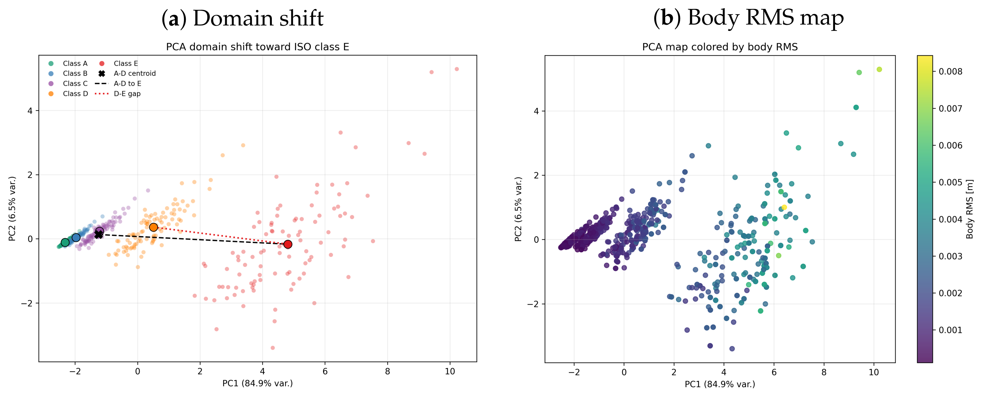
The one-second road-feature windows were projected onto two principal components to examine whether transfer failure is associated with measurable road-feature shift. The PCA map is used as a geometric diagnostic for the A–D to E transfer experiment, not only as a visual summary. Figure 2a shows an ordered road-severity structure: rougher classes move progressively away from smoother classes in the principal-component domain.

The centroid distances in

Table 3. PCA centroid distances between ISO road-feature domains. Distances are computed using non-suppressed one-second road-feature windows.

Comparison	PCA Centroid Distance
A–B	0.385
B–C	0.779
C–D	1.728
D–E	4.334
A–D centroid to E	6.067

quantify this separation. The A–B, B–C, and C–D distances are 0.385, 0.779, and 1.728 PCA units, respectively, whereas the D–E distance increases to 4.334 PCA units. The distance from the A–D training-domain centroid to class E is still larger, at 6.067 PCA units. Class E is not simply the next point on a smooth road-severity sequence; it is a substantially displaced target domain. This geometry is consistent with the later window-level transfer results, where A–D to E RTR becomes negative for body RMS, body peak, and tyre peak, and remains close to zero for tyre RMS.

The PCA distances in Table 3 provide the numerical counterpart of the feature-space map. The next figure is therefore used to show where these distances arise in the projected road-feature domain and how the same space relates to body-response magnitude.

The body-RMS overlay in Figure 2b shows that the displaced class-E region also contains the highest body-response magnitudes. In this sense, the PCA result produces an interpretable transfer result: the poor A–D to E performance is consistent with a road-feature domain-shift problem, not just with a weak regression model.

4.3. Domain Distance and Transferability

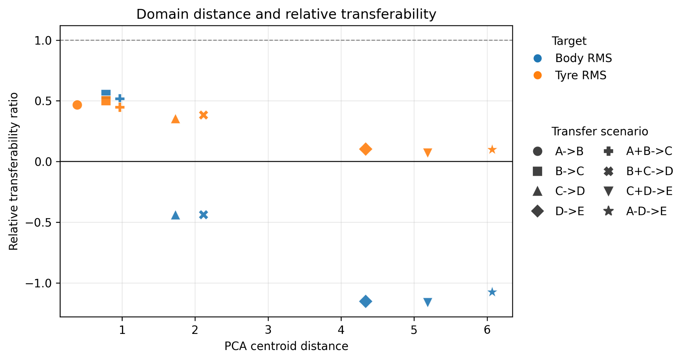
The PCA observation was tested more directly by relating domain-distance metrics to RTR across adjacent, graded, and broad transfer scenarios.

Table 4. Correlation between road-feature domain distance and RMS relative transferability ratio across window-level transfer scenarios.

Target	Distance Metric	Pearson r	95% CI	${\mathit{p}}_{\mathit{r}}$	Spearman $\mathit{\rho }$	${\mathit{p}}_{\mathit{\rho }}$	n
Body RMS	PCA centroid	−0.903	[−0.990, −0.830]	0.005	−0.857	0.014	7
Body RMS	Mahalanobis	0.098	[−0.723, 0.841]	0.835	−0.286	0.535	7
Body RMS	Mean Wasserstein	−0.904	[−0.990, −0.838]	0.005	−0.857	0.014	7
Tyre RMS	PCA centroid	−0.969	[−0.995, −0.915]	<$0.001$	−0.929	<$0.001$	8
Tyre RMS	Mahalanobis	0.262	[−0.509, 0.829]	0.531	0.000	1.000	8
Tyre RMS	Mean Wasserstein	−0.970	[−0.995, −0.925]	<$0.001$	−0.929	<$0.001$	8

reports the correlations for the RMS targets together with two-sided p-values and bootstrap confidence intervals. For both body RMS and tyre RMS, PCA centroid distance and mean Wasserstein distance show strong negative association with RTR. Mahalanobis distance is much less informative in this dataset. Because the number of transfer scenarios is small ($n=7$–8), these statistics should be read as diagnostic evidence rather than as a population-level inferential claim. Even so, the PCA and Wasserstein results consistently suggest that mean feature-domain separation is more relevant than covariance-normalized distance for this transfer problem.

Figure 3 shows the same relationship graphically. The class-E transfers occupy the high-distance and low-RTR region, especially for the window-level RMS targets. RTR is useful as a practical transfer diagnostic because performance loss is not randomly distributed across scenarios; it increases as the target road domain moves away from the training domain in feature space.

4.4. Sample-Level Transferability

Road-severity generalization was first evaluated with a leave-one-class-out protocol. For each ISO class, the model was trained on the remaining classes and tested on the held-out class. This is stricter than random sample splitting because it evaluates interpolation or extrapolation across road-severity conditions.

Table 5. Leave-one-road-class-out response prediction and relative transferability ratio (RTR).

Target	A		B		C		D		E
	${\mathit{R}}_{\mathrm{tr}}^{\mathbf{2}}$	RTR	${\mathit{R}}_{\mathrm{tr}}^{\mathbf{2}}$	RTR	${\mathit{R}}_{\mathrm{tr}}^{\mathbf{2}}$	RTR	${\mathit{R}}_{\mathrm{tr}}^{\mathbf{2}}$	RTR	${\mathit{R}}_{\mathrm{tr}}^{\mathbf{2}}$	RTR
Body displacement	0.608	0.655	0.358	0.376	0.533	0.554	0.860	0.977	0.736	0.982
Tyre displacement	0.833	0.887	0.944	0.972	0.939	0.956	0.939	0.984	0.818	0.959

shows that tyre displacement is more consistently transferable than body displacement. Tyre response has RTR values between 0.887 and 0.984, whereas body response drops to 0.376 for class B and 0.554 for class C. This difference is physically plausible. Tyre displacement lies closer to the road-input path and is more directly constrained by the measured excitation. Body displacement, in contrast, is filtered through sprung-mass motion, suspension compliance, damping, and frequency-dependent amplification or attenuation. It is therefore more sensitive to road-class-dependent changes in the dynamic response, while tyre displacement retains a stronger local relationship with the road signal. A model can consequently look accurate within individual road domains but lose a substantial fraction of its in-domain explanatory power when transferred. This is the central point of the study: aggregate prediction accuracy is incomplete unless road-class transfer is measured explicitly.

4.5. Window-Level Transferability

The next test moves from displacement samples to performance indices. One-second road windows were summarized using RMS, peak, standard deviation, peak-to-peak value, and road-band-power features. The evaluated scenarios were adjacent transfers, graded two-class transfers, and the broad transfer from classes A–D to class E.

Table 6. Adjacent, graded, and broad RMS transfer scenarios. RTR is not reported when the in-domain $R^2$ of the target class is non-positive.

Scenario	Body RMS		Tyre RMS
	${\mathit{R}}_{\mathrm{tr}}^{\mathbf{2}}$	RTR	${\mathit{R}}_{\mathrm{tr}}^{\mathbf{2}}$	RTR
A→B	−0.514	${\text{n.a.}}^{*}$	0.073	0.467
B→C	0.365	0.553	0.459	0.500
C→D	−0.322	−0.437	0.344	0.356
D→E	−0.364	−1.151	0.088	0.104
A + B→C	0.341	0.516	0.410	0.447
B + C→D	−0.322	−0.437	0.372	0.385
C + D→E	−0.367	−1.162	0.061	0.071
A–D→E	−0.340	−1.075	0.084	0.098

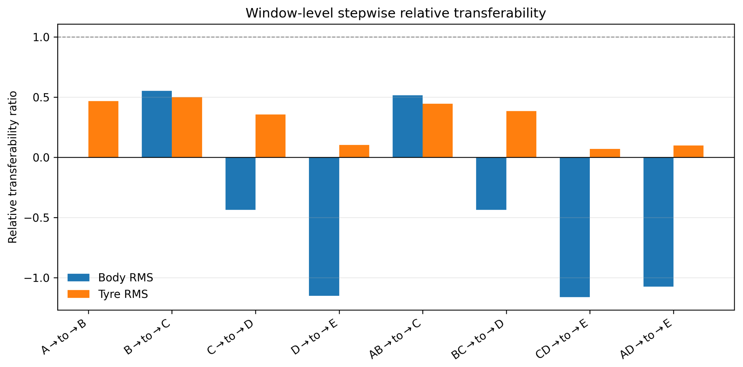
^* Not applicable because the in-domain $R^2$ of the target class was non-positive.

shows a clear weakening as the target class approaches E. The $D\to E$, $C+D\to E$, and A–D$\to E$ cases all yield negative or near-zero RTR for RMS targets, whereas $B\to C$ and $A+B\to C$ retain moderate positive RTR. The class-E failure is therefore not an artifact of using all A–D classes as training data; it is already visible in the adjacent $D\to E$ transfer. In the $A\to B$ body-RMS case, RTR is not reported, because the in-domain reference performance for the target class is non-positive. This behavior may be associated with the limited target variance of smooth-road conditions, where signal-to-noise ratio, measurement resolution, and quantization effects become relatively more influential.

The scenario-level values in Table 6 are easier to compare when plotted against transfer direction and target class. Figure 4 therefore emphasizes the same deterioration pattern visually before the broad class-E transfer case is isolated.

The broad A–D→E setting is reported separately because it corresponds to the most practical extrapolation question: whether a model trained on smoother and moderately rough roads remains reliable on the roughest class.

The weak and negative transfer $R^2$ values in

Table 7. Window-level broad transfer from ISO classes A–D to class E.

Target	${\mathit{R}}_{\mathbf{in}}^2$	${\mathit{R}}_{\mathbf{tr}}^2$	RTR	RMSE	NRMSE/RMS
Body RMS	0.316	−0.340	−1.075	0.001401	0.380
Tyre RMS	0.852	0.084	0.098	0.000970	0.285
Body peak	0.323	−0.694	−2.149	0.002922	0.405
Tyre peak	0.693	−0.808	−1.166	0.002675	0.364

are retained because they carry the main engineering message. Sample-level response prediction and window-level performance-index transfer are not equivalent. A model may reproduce displacement traces under leave-one-class-out testing while still failing to transfer aggregate RMS or peak indicators to a more severe road class. In other words, temporal fidelity in displacement reconstruction does not necessarily imply amplitude fidelity in window-level engineering indicators. This distinction matters for active-suspension diagnostics because design and monitoring decisions usually rely on RMS, peak, tyre-response, and comfort-related indices rather than on individual time samples. The class-E results therefore show that road-severity transfer must be assessed at the level of the engineering quantities that would actually support monitoring or control decisions.

Figure 5 summarizes the mean one-second window RMS values across ISO road classes and provides the response-amplitude context for the subsequent frequency-band analysis.

4.6. Frequency-Band Energy Analysis

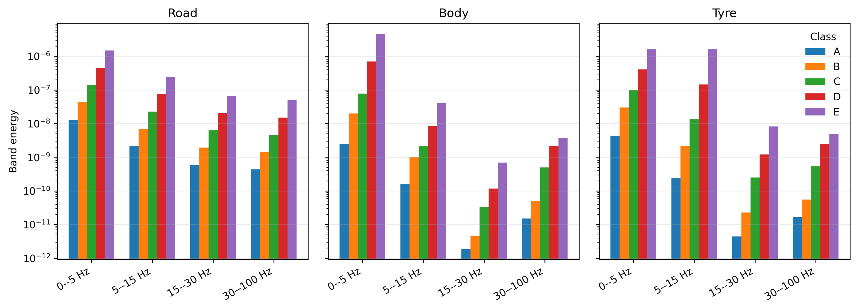
To interpret why class E is a difficult transfer target, road, body, and tyre responses were decomposed into four frequency bands.

Table 8. Class-E to class-D frequency-band energy ratios for non-suppressed signals.

Signal	0–5 Hz	5–15 Hz	15–30 Hz	30–100 Hz
Road	3.27	3.27	3.27	3.27
Body	6.57	4.80	5.84	1.75
Tyre	3.95	11.09	6.80	1.96

reports the E/D energy ratio. Road-input energy increases uniformly by a factor of 3.27 across the investigated bands, but response energy does not scale uniformly. Body response increases most strongly in the 0–5 Hz and 15–30 Hz bands, whereas tyre response shows a pronounced increase in the 5–15 Hz band. The E-class transfer problem is not only a larger input-amplitude problem; the response energy is redistributed across suspension-relevant bands.

The ratios in Table 8 summarize the class-E amplification relative to class D. Figure 6 then expands this comparison across all ISO classes, making clear that the class-E behavior is part of a broader but nonuniform energy-scaling pattern.

The different body and tyre energy shifts also explain why sample-level tyre displacement can remain more transferable than body displacement, while window-level tyre RMS transfer to E remains weak. The tyre signal is locally predictable from the road input, but its aggregate energy in the 5–15 Hz band changes sharply in class E. This distinction reinforces the need to evaluate both sample-level predictability and window-level performance transfer.

4.7. SHAP-Based Model Interpretation

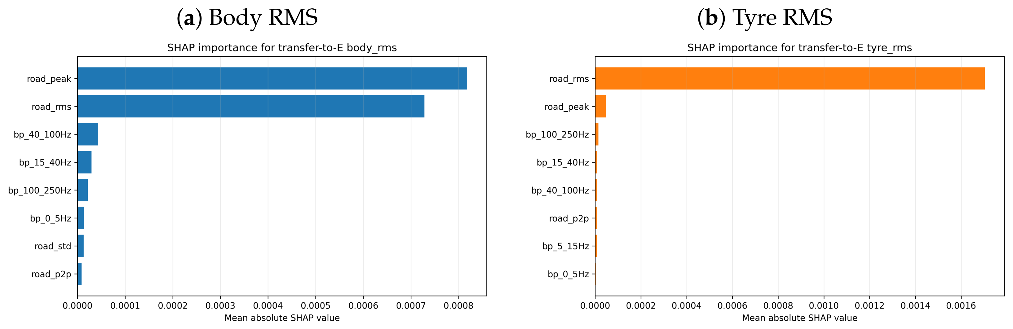
SHAP analysis was applied to the window-level models trained on classes A–D and evaluated on class E. For body RMS, the largest mean absolute SHAP values are associated with road peak and road RMS. For tyre RMS, road RMS dominates the explanation. The transfer models rely mainly on low-order road-amplitude descriptors rather than on a distributed frequency-band representation.

Table 9. Dominant SHAP features for A–D to E window-level RMS transfer.

Target	Feature	Mean Absolute SHAP Value
Body RMS	Road peak	0.000818
Body RMS	Road RMS	0.000728
Body RMS	40–100 Hz band power	0.0000436
Tyre RMS	Road RMS	0.001704
Tyre RMS	Road peak	0.0000466
Tyre RMS	100–250 Hz band power	0.0000143

identifies the dominant features by mean absolute SHAP value. The corresponding plots in Figure 7 show the relative feature contributions for the two RMS targets and help distinguish body-response and tyre-response dependence on road-amplitude descriptors. This does not contradict the frequency-band result in Table 8. The band-energy analysis describes how the physical response energy changes across road classes, whereas SHAP describes how the fitted transfer model distributes importance across the engineered input features. The low SHAP ranking of band-power features may therefore reflect the correlation with road RMS and road peak, or the dominance of those amplitude descriptors in the selected model, rather than proving that frequency-band changes are physically unimportant.

4.8. SOF Control-Effort Reconstruction

The SOF-controlled dataset was retained as a secondary check because it includes the measured control force, which is absent from the ISO benchmark. Under a blocked closed-loop split, $F_c$ was reconstructed from measured road and response variables with $R^2=0.99995$ using ridge regression and $R^2=0.99775$ using Extra Trees. This is consistent with the static-output-feedback nature of the controller and is not treated as the principal novelty of the paper. Its role is narrower: it shows that the control signal behaves as a structured and measurable response rather than as an unmodeled disturbance.

5. Limitations

The two datasets are not identical experimental records. They come from related Quanser active-suspension platform contexts but differ in excitation protocol, recorded variables, and available control information. The study avoids direct claims that one controller is superior to another across datasets. The SOF dataset is used only as a secondary control-effort consistency check because it does not contain the same ISO road-class structure as Dataset 2. In addition, Dataset 2 has already been used for road classification and resonant-system identification, and the present study deliberately avoids reproducing those contributions. Any acceleration-based comfort indicator computed from displacement signals would require filtering and sensitivity checks because numerical differentiation can amplify measurement noise. RTR is intentionally simple and should be interpreted as a comparative diagnostic ratio, not as a new universal index or as a replacement for full closed-loop validation under newly measured road profiles. Negative RTR values should be read as diagnostic evidence that transfer performance has fallen below the mean-prediction baseline, not as numerical errors. Conversely, when in-domain $R^2$ is non-positive, RTR is deliberately not reported, because the reference model does not provide a positive explanatory baseline. Such cases may be more likely under smooth-road, low-variance target conditions, where signal-to-noise ratio, measurement resolution, and quantization effects can become relatively more influential.

6. Conclusions

This study reframed Quanser-based active-suspension benchmark data around road-class generalization. Instead of treating high aggregate prediction accuracy as sufficient, it evaluated predictability, explainability, and transferability across ISO 8608 classes A–E. The ISO results show that tyre displacement transfers more consistently across unseen road classes than body displacement, while window-level RMS and peak indicators transfer poorly as the target domain approaches class E. RTR makes this degradation explicit: sample-level tyre-displacement models retain most of their in-domain performance, whereas class-E performance-index transfer can become weak or negative. Domain-distance analysis further shows that PCA centroid and Wasserstein distances are strongly negatively associated with RMS relative transferability, supporting the interpretation that class-E failure is a road-feature domain-shift problem. Frequency-band analysis indicates that class E does not merely scale the input uniformly; it produces disproportionate body and tyre response-energy increases in selected low- and mid-frequency bands. SHAP analysis complements this result by showing that road RMS and road peak dominate the A–D to E RMS transfer models. The SOF analysis remains a secondary check, showing that measured control force can be reconstructed with high accuracy under a static-output-feedback experiment. Overall, the contribution is an interpretable performance-assessment framework for road-severity transfer, not a new controller, road classifier, or system-identification method.