Effects of Uncertain Parameters on the Dynamic Response of a Wind Turbine Gearbox

Abstract

Producing reliable gear systems for wind turbines involves accounting for multiple uncertain parameters. To ensure operational vibrations remain controlled, it is essential to analyze the system’s sensitivity to these uncertainties. This study investigates the dynamic response of a two-stage wind turbine gear system, considering variations in many system variables. The goal is to evaluate the system’s reliability through bearing displacement analysis. A 12-DOF concentrated-parameter model is proposed to account for uncertainties in gear mass, damping, and the inertias of the pinion, gear, and input shaft. The dynamic response is examined using the Polynomial Chaos (PC) method across different orders and standard deviations, with results validated through the Monte Carlo (MC) method using 100,000 samples.

1. Introduction

Wind turbines vary in size depending on the desired energy production capacity. These systems generate electrical current for power stations or for self-consumption. Currently, a wind turbine is composed of three main parts: a horizontal-axis rotor, a nacelle, and a tower. Vibrations in one of these parts are propagated to the other through relative movements between mechanical parts such as shafts, gears, pinions, etc. [1]. In fact, gear transmission mechanisms are widely used for the connection and transfer of power in wind power generation. Due to heavy loads and harsh operating conditions, gear transmission mechanisms are likely to be subjected to severe vibrations. Therefore, along with advancements in industrial technology, the vibration characteristics of gear drive mechanisms must meet stringent performance requirements.

In-depth investigations into their dynamic responses offer valuable theoretical foundations for failure detection, performance optimization, and dependability assessment of gear-based power transmission systems [2,3]. Due to production and machining errors, material imperfections, degradation over time, environmental conditions, and several additional influences, certain mechanical properties such as weight, rigidity, and rotational resistance tend to exhibit variability [4,5,6]. To accurately assess the system’s dynamic performance, it is crucial to analyze the motion behavior of gear mechanisms under uncertain conditions. Various methods exist in the literature, among which Monte Carlo Simulation (MCS) is a widely used technique. MCS can provide the total probability density function of all the system variables, but it is generally considered to be costly because many samples are required to reach acceptable accuracy. Parallel simulation [7] and appropriate orthogonal decomposition [8] represent some solutions that have been considered to overcome the drawbacks associated with the MCS calculation. These techniques consist of solving the deterministic problem repeatedly for random parameter values and extracting the closest solution to this problem. The MCS technique is widely used in this field, but remains generally excessively expensive, as a significant number of samples is necessary to obtain satisfactory results.

To achieve information about the uncertainty in terms of first and second statistical moments quickly enough, the perturbation method is effective [9]. In this case, the statistical moments are determined by expanding the stochastic quantities around their mean via a Taylor series expansion. However, its use is limited to small perturbations. Alternatively, the Polynomial Chaos (PC) method [10,11] has proven effective in dealing with challenges associated with uncertainty. It is a development in orthogonal polynomials based on random variables, aimed at approximating the overall distribution of output uncertainty. The main homogeneous Polynomial Chaos method is founded on Wiener’s homogeneous chaos theory. It utilizes Hermite polynomials in conjunction with Gaussian random variables. The effectiveness of this approach has been demonstrated in various application fields, particularly in managing uncertainties in environmental and biological phenomena [12,13] and multi-body dynamical systems [14,15,16,17], the solution of ordinary and partial differential equations, and parameter estimation.

Many studies have investigated the reliability of vibrating structures while considering uncertainties. Guerine and El Hami [1] examined the nonlinear dynamic behavior of a mechanical torque limiter designed to safeguard drivetrain components such as helical transmission gears against overload. In a previous study, Guerine et al. (2017) [18] analyzed the dynamic response of wind turbine gear systems with uncertain yet bounded parameters, employing the interval analysis method. They also studied the stability of an eight-degree-of-freedom spur gear according to the coefficient of friction value. Wang et al. (2021) [19] studied an uncertain transient response of the dual disk rotor system using a non-probabilistic Chebyshev convex method (CCM). Zhou et al. (2018) [20] have studied a nonlinear coupled lateral-torsional dynamic model with 16 degrees of freedom for the gear-rotor-bearing system. They have considered nonlinear characteristics such as variable gear stiffness, backlash, transmission error, and friction force. Their research focused on the effects of the friction coefficient and mean load, revealing the complex influence of these factors on the behavior of the gear system. Giannella (2021) [21] presented a stochastic model, which considers various sources of uncertainty, to define the probability distribution of the residual fatigue life of a defective railway axle. Garoli and Castro (2019) [22] considered the consequences of temperature uncertainty on the dynamic coefficient of the bearing using the PC to solve the problem of the vortex instability of the oil film of the rotor-bearing system. To address the issue of reliability, specifically the estimation of very low exceedance probabilities, Wang and Zhang (2021) [23] analyzed the effect of stochastic interval variables such as meshing rigidity, driving moment, kinematic inaccuracy, and backlash on the oscillatory velocity spectrum and operational dependability of gear train mechanisms. In their research, the dynamic system incorporating interval uncertainties was resolved through the integration of the Chebyshev enclosure function technique and the Runge–Kutta numerical integration algorithm.

In addition, it should be noted that the literature has not thoroughly investigated the dynamic behavior of a two-stage gearbox used in wind turbines, particularly with the presence of uncertain parameters. Furthermore, most studies have only focused on analyzing a few uncertain parameters, such as the input torque or the mesh stiffness. However, to the best of our knowledge, there is a lack of research that considers the simultaneous effects of multiple uncertain parameters. In this study, we have considered many uncertain parameters that have a significant impact on the dynamic response of the gearbox. Therefore, this research contributes to addressing this gap in the literature by providing a comprehensive analysis of the dynamic behavior of a two-stage gearbox under uncertainty, considering multiple uncertain parameters. In addition, the literature offers several approaches to addressing uncertainty, typically classified into four main categories. The first category is the deterministic MCS approach, which is commonly used as a reference due to its ability to produce reliable results that are close to reality. However, the MCS can be computationally intensive, limiting its applicability. To minimize the computational cost of simulations with uncertainties, other probabilistic approaches have been developed, such as the perturbation method, PC method, and the meta-model method. These methods provide efficient ways to generate accurate results. Finally, the literature also includes a possibilistic approach, such as the interval computing method. These methods provide an alternative framework for addressing uncertainty and offer valuable insight into various fields of study.

This study presents a proposed approach to model the dynamic behavior of a two-stage gearbox used in a horizontal wind turbine while accounting for uncertainties related to the mass, the moment of inertia, the bearing’s bending stiffness, the traction-compression stiffness, the damping coefficient, and the wind speeds. The main innovation of this study lies in its ambitious approach to include as many parameters as possible that could potentially contribute to the random vibrations of the system and to set it apart from the existing literature. By comprehensively analyzing this large number of variables and considering three different standard deviations, our aim is to obtain a more realistic understanding of the behavior and operation of the studied system in the face of varying uncertainty conditions. Furthermore, by studying the effects of multiple sources of uncertainty on the system’s random vibrations with different standard deviations, we can define their influence on the dynamic response and identify the critical thresholds where the system’s behavior could be most sensitive to uncertainty variations. In this way, this approach provides a better understanding of the standard deviation thresholds that affect system robustness and stability under real operating conditions and directs our efforts towards improving the design to minimize the negative effects of undesirable standard deviations on system performance.

2. Overview of Mechanical Architecture

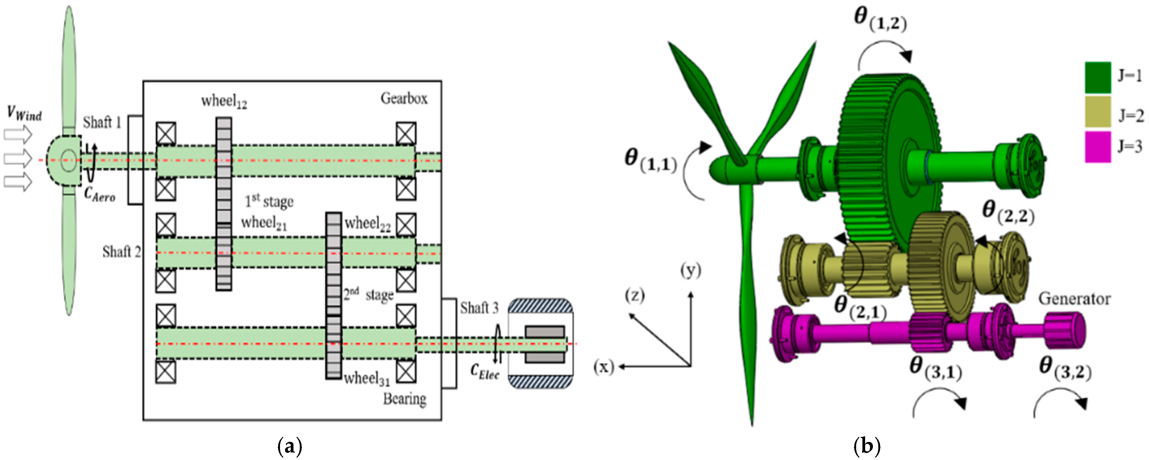
A wind energy conversion system is a rotary apparatus that extracts kinetic energy from a fluid medium (i.e., atmospheric airflow) via aerodynamic airfoils and transduces it into utilizable mechanical power [24]. Figure 1 illustrates the nonlinear dynamic representation of the analyzed horizontal-axis wind turbine (HAWT). The rotor assembly typically consists of a tri-blade configuration affixed to a central hub, which is mechanically coupled to a speed-increasing gearbox through a transmission shaft supported by an initial compliant bearing element.

The comprehensive dynamic formulation is composed of three subsystems $\left(\mathrm{j} = 1, \dots , 3\right)$, each supported by a compliant bearing assembly. For the first subsystem, the lateral (bending) stiffness of the bearing is denoted by ${\mathrm{k}}_1^{\mathrm{x}}$, and the axial (traction-compression) stiffness is designated as ${\mathrm{k}}_1^{\mathrm{y}}$. Analogously, for the second subsystem, the stiffness parameters are ${\mathrm{k}}_2^{\mathrm{x}}$ and ${\mathrm{k}}_2^{\mathrm{y}}$. Meanwhile, for the third subsystem, they are represented as ${\mathrm{k}}_3^{\mathrm{x}}$ and ${\mathrm{k}}_3^{\mathrm{y}}$. The interconnecting shafts among these blocks exhibit torsional rigidity, quantified by ${\mathrm{k}}_1^{\mathsf{\theta }}$, ${\mathrm{k}}_2^{\mathsf{\theta }}$ and ${\mathrm{k}}_3^{\mathsf{\theta }}$. It is assumed that the intermediate flexible couplings possess negligible inertial mass relative to that of the gearbox assembly. The angular displacements associated with each rotational component are denoted respectively as ${\mathsf{\theta }}_{\left(11\right)}$, ${\mathsf{\theta }}_{\left(1,2\right)}$, ${\mathsf{\theta }}_{\left(2,1\right)}{\mathsf{\theta }}_{\left(2,2\right)}$, ${\mathsf{\theta }}_{\left(3,1\right)}$ and ${\mathsf{\theta }}_{\left(3,2\right)}$. Moreover, the translational displacements of the bearing supports, in the plane orthogonal to the axis of rotation, are expressed as ${\mathrm{x}}_1$ and ${\mathrm{y}}_1$ for the first subsystem, ${\mathrm{x}}_2$ and ${\mathrm{y}}_2$ for the second, ${\mathrm{x}}_3$ and ${\mathrm{y}}_3$ for the third.

3. Equations of Motion

The dynamic behavior of the investigated system (Figure 1) is governed by the equations of motion formulated via the Lagrangian approach. These equations are represented in the canonical matrix format as follows:

$$\left[\mathrm{M}\right]\left\{\ddot{\mathrm{q}}\right\}+\left[\mathrm{C}\right]\left\{\dot{\mathrm{q}}\right\}+\left(\left[{\mathrm{K}}_{\mathrm{S}}\right]+\left[\mathrm{K}\left(\mathrm{t}\right)\right]\right)\left\{\mathrm{q}\right\}=\left\{{\mathrm{F}}_{\mathrm{e}\mathrm{x}\mathrm{t}}\right\}$$

(1)

where

$$\left\{\mathrm{q}\left(\mathrm{t}\right)\right\}={\left\{{\mathrm{x}}_1,{\mathrm{y}}_1,{\mathrm{x}}_2,{\mathrm{y}}_2,{\mathrm{x}}_3,{\mathrm{y}}_3,{\mathsf{\theta }}_{11},{\mathsf{\theta }}_{12},{\mathsf{\theta }}_{21},{\mathsf{\theta }}_{22},{\mathsf{\theta }}_{31},{\mathsf{\theta }}_{32}\right\}}^{\mathrm{T}}$$

(2)

$⟨{\mathrm{L}}_{\mathsf{\delta }\mathrm{n}}⟩$ is a function of the n-level.

$$⟨{\mathrm{L}}_{\mathsf{\delta }1}⟩=\left[-\sin \left({\mathsf{\alpha }}_1\right),\cos \left({\mathsf{\alpha }}_1\right),\sin \left({\mathsf{\alpha }}_1\right),-\cos \left({\mathsf{\alpha }}_1\right),\mathrm{0,0},0,{\mathrm{r}}_{12}^{\mathrm{b}},{\mathrm{r}}_{21}^{\mathrm{b}},\mathrm{0,0},0\right]$$

(3)

$$⟨{\mathrm{L}}_{\mathsf{\delta }2}⟩=\left[-\sin \left({\mathsf{\alpha }}_2\right),\cos \left({\mathsf{\alpha }}_2\right),\sin \left({\mathsf{\alpha }}_2\right),-\cos \left({\mathsf{\alpha }}_2\right),\mathrm{0,0},0,{\mathrm{r}}_{22}^{\mathrm{b}},{\mathrm{r}}_{31}^{\mathrm{b}},\mathrm{0,0},0\right]$$

(4)

The parameters ${\mathrm{r}}_{12}^{\mathrm{b}}$ and ${\mathrm{r}}_{21}^{\mathrm{b}}$ denote the base radii of gears (12) and (21), respectively. Similarly, ${\mathrm{r}}_{22}^{\mathrm{b}}$ and ${\mathrm{r}}_{31}^{\mathrm{b}}$ correspond to the base radii of gears (22) and (31), respectively. The pressure angles associated with the first and second gear stages are represented by ${\mathsf{\alpha }}_1$ and ${\mathsf{\alpha }}_2$, respectively.

The global mass matrix of the mechanical system is expressed in the following block matrix form:

$$\left[{\mathrm{M}}_{\mathrm{G}}\right]=\left[\begin{array}{cc}{\mathrm{M}}_{\mathrm{L}}& 0\\ 0& {\mathrm{M}}_{\mathrm{A}}\end{array}\right]$$

(5)

Here, $\left[{\mathrm{M}}_{\mathrm{L}}\right]$ denotes the mass matrix associated with the rotating components (wheels), and is defined as:

$$\left[{\mathrm{M}}_{\mathrm{L}}\right]=\mathrm{d}\mathrm{i}\mathrm{a}\mathrm{g}\left({\mathrm{m}}_1,{\mathrm{m}}_1,{\mathrm{m}}_{2,}{\mathrm{m}}_2,{\mathrm{m}}_3,{\mathrm{m}}_3\right)$$

(6)

${\mathrm{m}}_{\mathrm{j}}$ is the mass of the bloc j.

$\left[{\mathrm{M}}_{\mathrm{A}}\right]$ is the matrix of inertia and is written as follows:

$$\left[{\mathrm{M}}_{\mathrm{A}}\right]=\mathrm{d}\mathrm{i}\mathrm{a}\mathrm{g}\left({\mathrm{I}}_{11},{\mathrm{I}}_{12},{\mathrm{I}}_{21},{\mathrm{I}}_{22},{\mathrm{I}}_{31},{\mathrm{I}}_{32}\right)$$

(7)

${\mathrm{I}}_{\mathrm{ji}}$ are the polar inertia of the Wheel (ji) relative to the axis of rotation.

To attenuate the vibratory response of the system, a proportional damping matrix $\left[\mathrm{C}\right]$ was implemented, following the methodology outlined in [24,25].

$$\left[\mathrm{C}\right]=\mathsf{\eta }\left[\mathrm{M}\right]+\mathsf{\mu }\left(\left[{\mathrm{K}}_{\mathrm{S}}+\left[{\mathrm{K}}_{\mathrm{c}}\right]\right]\right)$$

(8)

where $\left[{\mathrm{K}}_{\mathrm{c}}\right]$ is the mean component of mesh stiffness.

With: $\mathsf{\eta }$ and $\mathsf{\mu }$ are the damping constants defined by: $\mathsf{\eta }=10^{-2};\mathsf{\mu }=10^{-5}$ [25].

The global stiffness matrix $\left[{\mathrm{K}}_{\mathrm{s}}\right]$ is constructed from the superposition of the mean structural stiffness matrix, the torsional rigidity matrix $\left[{\mathrm{K}}_{\mathsf{\theta }}\right]$ of the interconnecting shafts, and the elastic stiffness matrix of the bearing $\left[{\mathrm{K}}_{\mathrm{p}}\right]$ assemblies [25].

$$\left[{\mathrm{K}}_{\mathrm{s}}\right]=\left[\begin{array}{cc}{\mathrm{K}}_{\mathrm{p}}& 0\\ 0& {\mathrm{K}}_{\mathsf{\theta }}\end{array}\right]$$

(9)

The gear-mesh stiffness matrix $\left[\mathrm{K}\left(\mathrm{t}\right)\right]$ is expressed by:

$$\left[\mathrm{K}\left(\mathrm{t}\right)\right]=\left[\begin{array}{cc}\left[{\mathrm{K}}_1\left(\mathrm{t}\right)\right]& \left[{\mathrm{K}}_{12}\left(\mathrm{t}\right)\right]\\ \left[{\mathrm{K}}_{12}^{\mathrm{T}}\left(\mathrm{t}\right)\right]& \left[{\mathrm{K}}_2\left(\mathrm{t}\right)\right]\end{array}\right]$$

(10)

With

$$\left[{\mathrm{K}}_1\left(\mathrm{t}\right)\right]=\left[\begin{array}{cccccc}{\mathrm{k}}_1{\mathrm{x}}_1^2& -{\mathrm{k}}_1\dot{\mathrm{x}}& -{\mathrm{k}}_1{\mathrm{x}}_1^2& {\mathrm{k}}_1\dot{\mathrm{x}}& 0& 0\\ {\mathrm{k}}_1\dot{\mathrm{x}}& {\mathrm{k}}_1{\dot{\mathrm{y}}}^2& {\mathrm{k}}_1\dot{\mathrm{x}}& -{\mathrm{k}}_1{\dot{\mathrm{x}}}^2& 0& 0\\ -{\mathrm{k}}_1{\mathrm{x}}_1^2& {\mathrm{k}}_1\dot{\mathrm{x}}& {\mathrm{k}}_1{\mathrm{x}}_1^2+{\mathrm{k}}_2{\mathrm{x}}_2^2& -{\mathrm{k}}_1\dot{\mathrm{x}}-{\mathrm{k}}_2\ddot{\mathrm{x}}& -{\mathrm{k}}_2{\mathrm{x}}_2^2& {\mathrm{k}}_2\ddot{\mathrm{x}}\\ {\mathrm{k}}_1\dot{\mathrm{x}}& {\mathrm{k}}_1{\dot{\mathrm{y}}}^2& -{\mathrm{k}}_1\dot{\mathrm{x}}-{\mathrm{k}}_2\ddot{\mathrm{x}}& {\mathrm{k}}_1{\dot{\mathrm{y}}}^2+{\mathrm{k}}_2{\dot{\mathrm{y}}}^2& {\mathrm{k}}_2\ddot{\mathrm{x}}& {\mathrm{k}}_2{\ddot{\mathrm{y}}}^2\\ 0& 0& -{\mathrm{k}}_2{\mathrm{x}}_2^2& {\mathrm{k}}_2\ddot{\mathrm{x}}& {\mathrm{k}}_2{\mathrm{x}}_2^2& -{\mathrm{k}}_2\ddot{\mathrm{x}}\\ 0& 0& {\mathrm{k}}_2\ddot{\mathrm{x}}& {\mathrm{k}}_2{\ddot{\mathrm{y}}}^2& {\mathrm{k}}_2\ddot{\mathrm{x}}& {\mathrm{k}}_2{\ddot{\mathrm{y}}}^2\end{array}\right]$$

(11)

$$\left[{\mathrm{K}}_{12}\left(\mathrm{t}\right)\right]=\left[\begin{array}{cccccc}0& {\mathrm{k}}_1{\mathrm{r}}_{12}^{\mathrm{b}}{\mathrm{x}}_1& {\mathrm{k}}_1{\mathrm{r}}_{21}^{\mathrm{b}}{\mathrm{x}}_1& 0& 0& 0\\ 0& {\mathrm{k}}_1{\mathrm{r}}_{12}^{\mathrm{b}}\dot{\mathrm{y}}& {\mathrm{k}}_1{\mathrm{r}}_{21}^{\mathrm{b}}\dot{\mathrm{y}}& 0& 0& 0\\ 0& {\mathrm{k}}_1{\mathrm{r}}_{21}^{\mathrm{b}}{\mathrm{x}}_1& {\mathrm{k}}_1{\mathrm{r}}_{12}^{\mathrm{b}}{\mathrm{x}}_1& {\mathrm{k}}_2{\mathrm{r}}_{22}^{\mathrm{b}}{\mathrm{x}}_2& {\mathrm{k}}_2{\mathrm{r}}_{31}^{\mathrm{b}}{\mathrm{x}}_2& 0\\ 0& -{\mathrm{k}}_1{\mathrm{r}}_{12}^{\mathrm{b}}\dot{\mathrm{y}}& -{\mathrm{k}}_1{\mathrm{r}}_{21}^{\mathrm{b}}\dot{\mathrm{y}}& -{\mathrm{k}}_2{\mathrm{r}}_{22}^{\mathrm{b}}\ddot{\mathrm{y}}& -{\mathrm{k}}_2{\mathrm{r}}_{31}^{\mathrm{b}}\ddot{\mathrm{y}}& 0\\ 0& 0& 0& -{\mathrm{k}}_2{\mathrm{r}}_{22}^{\mathrm{b}}{\mathrm{x}}_2& -{\mathrm{k}}_2{\mathrm{r}}_{31}^{\mathrm{b}}{\mathrm{x}}_2& 0\\ 0& 0& 0& {\mathrm{k}}_2{\mathrm{r}}_{22}^{\mathrm{b}}\ddot{\mathrm{y}}& {\mathrm{k}}_2{\mathrm{r}}_{31}^{\mathrm{b}}\ddot{\mathrm{y}}& 0\end{array}\right]$$

(12)

$$\left[{\mathrm{K}}_2\left(\mathrm{t}\right)\right]=\left[\begin{array}{cccccc}0& 0& 0& 0& 0& 0\\ 0& {\mathrm{k}}_1{\mathrm{r}}_{12}^{\mathrm{b}}& {\mathrm{k}}_1{\mathrm{r}}_{12}^{\mathrm{b}}{\mathrm{r}}_{21}^{\mathrm{b}}& 0& 0& 0\\ 0& {\mathrm{k}}_1{\mathrm{r}}_{12}^{\mathrm{b}}{\mathrm{r}}_{21}^{\mathrm{b}}& {\mathrm{k}}_1{\mathrm{r}}_{21}^{\mathrm{b}}& 0& 0& 0\\ 0& 0& 0& {\mathrm{k}}_2{\mathrm{r}}_{22}^{\mathrm{b}}& {\mathrm{k}}_2{\mathrm{r}}_{22}^{\mathrm{b}}{\mathrm{r}}_{31}^{\mathrm{b}}& 0\\ 0& 0& 0& {\mathrm{k}}_2{\mathrm{r}}_{22}^{\mathrm{b}}{\mathrm{r}}_{31}^{\mathrm{b}}& {\mathrm{k}}_2{\mathrm{r}}_{31}^{\mathrm{b}}& 0\\ 0& 0& 0& 0& 0& 0\end{array}\right]$$

(13)

where

$\left[{\mathrm{K}}_1\left(\mathrm{t}\right)\right]$ is the first-time varying stiffness.

$\left[{\mathrm{K}}_2\left(\mathrm{t}\right)\right]$ is the second-time varying stiffness.

$${\mathrm{x}}_1=\sin \left({\mathsf{\alpha }}_1\right),{\mathrm{x}}_2=\sin \left({\mathsf{\alpha }}_2\right),\dot{\mathrm{x}}=\left(\sin \left({\mathsf{\alpha }}_1\right)\cos \left({\mathsf{\alpha }}_1\right)\right),\ddot{\mathrm{x}}=\left(\sin \left({\mathsf{\alpha }}_2\right)\cos \left({\mathsf{\alpha }}_2\right)\right),\dot{\mathrm{y}}=\cos \left({\mathsf{\alpha }}_1\right),\ddot{\mathrm{y}}=\cos \left({\mathsf{\alpha }}_2\right)$$

The external vector force is defined by:

$$\left\{{\mathrm{F}}_{\mathrm{e}\mathrm{x}\mathrm{t}}\right\}={\left\{\mathrm{0,0},\mathrm{0,0},\mathrm{0,0},{\mathrm{C}}_{\mathrm{a}\mathrm{e}\mathrm{r}}\left(\mathrm{t}\right),\mathrm{0,0},\mathrm{0,0},{\mathrm{C}}_{\mathrm{g}\mathrm{e}\mathrm{n}}\left(\mathrm{t}\right)\right\}}^{\mathrm{T}}$$

(14)

where ${\mathrm{C}}_{\mathrm{a}\mathrm{e}\mathrm{r}}\left(\mathrm{t}\right)$ is the aerodynamic torque and ${\mathrm{C}}_{\mathrm{g}\mathrm{e}\mathrm{n}}\left(\mathrm{t}\right)$ is the generator torque.

Under ideal operational conditions, the system is subjected to both external and internal excitation sources. The primary contributors to these dynamic excitations include the stochastic variability of the wind energy input and the time-dependent fluctuation of the gear meshing stiffness [25]. In the current investigation, only aerodynamic excitation due to wind variability is considered [26]. Therefore, the wind turbine speed ${\mathsf{\Omega }}_{\mathrm{w}\left(\mathrm{t}\right)}$ is considered a fixed value for an average level of wind magnitude.

The wind velocity is expressed as follows [25].

$${\mathrm{V}}_{\mathrm{w}\mathrm{i}\mathrm{n}}\left(\mathrm{t}\right)={\mathrm{V}}_{\mathrm{m}\mathrm{o}\mathrm{y}}$$

(15)

where $({\mathsf{\omega }}_1 = \mathsf{\pi })$ and $({\mathsf{\omega }}_2 = 2\mathsf{\pi })$ represent the angular frequencies (rad/s).

Under these operating conditions, the instantaneous aerodynamic torque is defined as follows:

$${\mathrm{C}}_{\mathrm{a}\mathrm{e}\mathrm{r}}(\mathrm{t})={\displaystyle \frac{1}{2{\mathsf{\Omega }}_{\mathrm{w}\left(\mathrm{t}\right)}}}\mathsf{\pi }{\mathsf{\rho }}_{\mathrm{a}\mathrm{i}\mathrm{r}}{\mathrm{R}}^2{\mathrm{V}}_{\mathrm{w}\mathrm{i}\mathrm{n}\left(\mathrm{t}\right)}^3{\mathrm{C}}_{\mathrm{p}}$$

(16)

where

${\mathrm{C}}_{\mathrm{p}}$, $R$ and ${\mathsf{\rho }}_{\mathrm{air}}$ represent, respectively, the power coefficient, the rotor radius, and the air density.

The generator torque ${\mathrm{C}}_{\mathrm{g}\mathrm{e}\mathrm{n}}\left(\mathrm{t}\right)$ is dependent on the aerodynamic torque ${\mathrm{C}}_{\mathrm{a}\mathrm{e}\mathrm{r}}\left(\mathrm{t}\right)$ and the gearbox ratio. It is defined by:

$${\mathrm{C}}_{\mathrm{g}\mathrm{e}\mathrm{n}}(\mathrm{t})={\displaystyle \frac{-{\mathrm{C}}_{\mathrm{a}\mathrm{e}\mathrm{r}}\left(\mathrm{t}\right)}{{\mathsf{\eta }}_{\mathrm{g}\mathrm{e}\mathrm{a}\mathrm{r}}}}$$

(17)

where ${\mathsf{\eta }}_{\mathrm{g}\mathrm{e}\mathrm{a}\mathrm{r}}$ represent the gear ratio and is calculated as follows:

$${\mathsf{\eta }}_{\mathrm{g}\mathrm{e}\mathrm{a}\mathrm{r}}={\displaystyle \frac{{\mathrm{Z}}_{12}{\mathrm{Z}}_{21}}{{\mathrm{Z}}_{22}{\mathrm{Z}}_{31}}}$$

(18)

With

${\mathrm{Z}}_{12}$, ${\mathrm{Z}}_{21}$, ${\mathrm{Z}}_{22}$ and ${\mathrm{Z}}_{31}$ are the teeth number of n gear stage.

The motion of the wind turbine blocks, which involve both linear and torsional displacements, can be mathematically described by a system of differential equations, as presented below.

$$|\begin{array}{l}m{\ddot{\mathrm{x}}}_1-{\mathrm{c}}^{\mathrm{x}}{\dot{\mathrm{x}}}_1+\sin \left({\mathsf{\alpha }}_1\right){\mathrm{c}}_1{\mathsf{\delta }}_1\left(\mathrm{t}\right)+{\mathrm{k}}^{\mathrm{x}}{\mathrm{x}}_1-{\mathrm{k}}_1{\mathsf{\delta }}_1\left(\mathrm{t}\right)\sin \left({\mathsf{\alpha }}_1\right)=0\\ m{\ddot{\mathrm{y}}}_1-{\mathrm{c}}^{\mathrm{y}}{\dot{\mathrm{y}}}_1+\cos ({\mathsf{\alpha }}_1\left){\mathrm{c}}_1\right(t\left){\mathsf{\delta }}_1\right(t)+{\mathrm{k}}^{\mathrm{y}}{\mathrm{y}}_1+{\mathrm{k}}_1(t\left){\mathsf{\delta }}_1\right(t\left)\cos ({\mathsf{\alpha }}_1\right)=0\\ m{\ddot{\mathrm{x}}}_2+{\mathrm{c}}^{\mathrm{x}}{\dot{\mathrm{x}}}_2-\sin ({\mathsf{\alpha }}_1\left){\mathrm{c}}_1\right(t\left){\mathsf{\delta }}_1\right(t)+\sin ({\mathsf{\alpha }}_2){\mathrm{c}}_2\left(t\right){\mathsf{\delta }}_2\left(t\right)+{\mathrm{k}}^{\mathrm{x}}{\mathrm{x}}_2-{\mathrm{k}}_1\left(t\right)\sin ({\mathsf{\alpha }}_1)+{\mathrm{k}}_2(t\left)\sin ({\mathsf{\alpha }}_2\right){\mathsf{\delta }}_2\left(t\right)=0\\ m{\ddot{\mathrm{y}}}_2+{\mathrm{c}}^{\mathrm{y}}{\dot{\mathrm{y}}}_2-{\mathrm{k}}_1\left(t\right){\mathsf{\delta }}_1\left(t\right)\cos ({\mathsf{\alpha }}_1)+\cos ({\mathsf{\alpha }}_2){\mathrm{c}}_2\left(t\right){\mathsf{\delta }}_2\left(t\right)+{\mathrm{k}}^{\mathrm{y}}{\mathrm{y}}_2-{\mathrm{k}}_1\left(t\right)\cos ({\mathsf{\alpha }}_1\left){\mathsf{\delta }}_1\right(t)+{\mathrm{k}}_2(t\left){\mathsf{\delta }}_2\right(t\left)\cos ({\mathsf{\alpha }}_2\right)=0\\ m{\ddot{\mathrm{x}}}_3-{\mathrm{c}}^{\mathrm{x}}{\dot{\mathrm{x}}}_3-\sin ({\mathsf{\alpha }}_2\left){\mathrm{c}}_2\right(t\left){\mathsf{\delta }}_2\right(t)+{\mathrm{k}}^{\mathrm{x}}{\mathrm{x}}_3-{\mathrm{k}}_2(t\left){\mathsf{\delta }}_2\sin ({\mathsf{\alpha }}_2\right)=0\\ m{\ddot{\mathrm{y}}}_3-{\mathrm{c}}^{\mathrm{y}}{\dot{\mathrm{y}}}_3-\cos ({\mathsf{\alpha }}_2\left){\mathrm{c}}_2\right(t\left){\mathsf{\delta }}_2\right(t)+{\mathrm{k}}^{\mathrm{y}}{\mathrm{y}}_3-{\mathrm{k}}_2(t\left){\mathsf{\delta }}_2\cos ({\mathsf{\alpha }}_2\right)=0\end{array}$$

(19)

$$|\begin{array}{l}{\mathrm{I}}_{\mathrm{b}}{\ddot{\mathsf{\theta }}}_{\left(\mathrm{1,1}\right)}+{\mathrm{k}}^{\mathsf{\theta }}({\mathsf{\theta }}_{\left(\mathrm{1,1}\right)}-{\mathsf{\theta }}_{\left(\mathrm{1,2}\right)})={\mathrm{C}}_{\mathrm{a}\mathrm{é}\mathrm{r}\mathrm{o}}\left(t\right)\\ {\mathrm{I}}_{\left(\mathrm{1,2}\right)}{\ddot{\mathsf{\theta }}}_{\left(\mathrm{1,2}\right)}+{\mathrm{r}}_{\left(\mathrm{1,2}\right)}^{\mathrm{b}}{\mathrm{c}}_1\left(t\right){\mathsf{\delta }}_1\left(t\right)-{\mathrm{k}}^{\mathsf{\theta }}({\mathsf{\theta }}_{\left(\mathrm{1,1}\right)}-{\mathsf{\theta }}_{\left(\mathrm{1,2}\right)})+{\mathrm{k}}_1\left(t\right){\mathrm{r}}_{\left(\mathrm{1,2}\right)}^{\mathrm{b}}{\mathsf{\delta }}_1\left(t\right)=0\\ {\mathrm{I}}_{\left(\mathrm{2,1}\right)}{\ddot{\mathsf{\theta }}}_{\left(\mathrm{2,1}\right)}+{\mathrm{r}}_{\left(\mathrm{2,1}\right)}^{\mathrm{b}}{\mathrm{c}}_1\left(t\right){\mathsf{\delta }}_1\left(t\right)-{\mathrm{k}}^{\mathsf{\theta }}({\mathsf{\theta }}_{\left(\mathrm{2,1}\right)}-{\mathsf{\theta }}_{\left(\mathrm{2,2}\right)})+{\mathrm{k}}_1\left(t\right){\mathrm{r}}_{\left(\mathrm{2,1}\right)}^{\mathrm{b}}{\mathsf{\delta }}_1\left(t\right)=0\\ {\mathrm{I}}_{\left(\mathrm{2,2}\right)}{\ddot{\mathsf{\theta }}}_{\left(\mathrm{2,2}\right)}+{\mathrm{r}}_{\left(\mathrm{2,2}\right)}^{\mathrm{b}}{\mathrm{c}}_2\left(t\right){\mathsf{\delta }}_2\left(t\right)-{\mathrm{k}}^{\mathsf{\theta }}({\mathsf{\theta }}_{\left(\mathrm{2,1}\right)}-{\mathsf{\theta }}_{\left(\mathrm{2,2}\right)})+{\mathrm{k}}_2\left(t\right){\mathrm{r}}_{\left(\mathrm{2,2}\right)}^{\mathrm{b}}{\mathsf{\delta }}_2\left(t\right)=0\\ {\mathrm{I}}_{\left(\mathrm{3,1}\right)}{\ddot{\mathsf{\theta }}}_{\left(\mathrm{3,1}\right)}+{\mathrm{r}}_{\left(\mathrm{3,1}\right)}^{\mathrm{b}}{\mathrm{c}}_2\left(t\right){\mathsf{\delta }}_2\left(t\right)-{\mathrm{k}}^{\mathsf{\theta }}({\mathsf{\theta }}_{\left(\mathrm{2,2}\right)}-{\mathsf{\theta }}_{\left(\mathrm{3,1}\right)})+{\mathrm{k}}_2\left(t\right){\mathrm{r}}_{\left(\mathrm{3,1}\right)}^{\mathrm{b}}{\mathsf{\delta }}_2\left(t\right)=0\\ {\mathrm{I}}_{\mathrm{b}}{\ddot{\mathsf{\theta }}}_{\left(\mathrm{3,2}\right)}+{\mathrm{k}}^{\mathsf{\theta }}({\mathsf{\theta }}_{\left(\mathrm{3,1}\right)}-{\mathsf{\theta }}_{\left(\mathrm{3,2}\right)})=-{\mathrm{C}}_{\mathrm{r}}\left(t\right)\end{array}$$

(20)

4. Uncertainty Methods

4.1. Monte Carlo Simulation

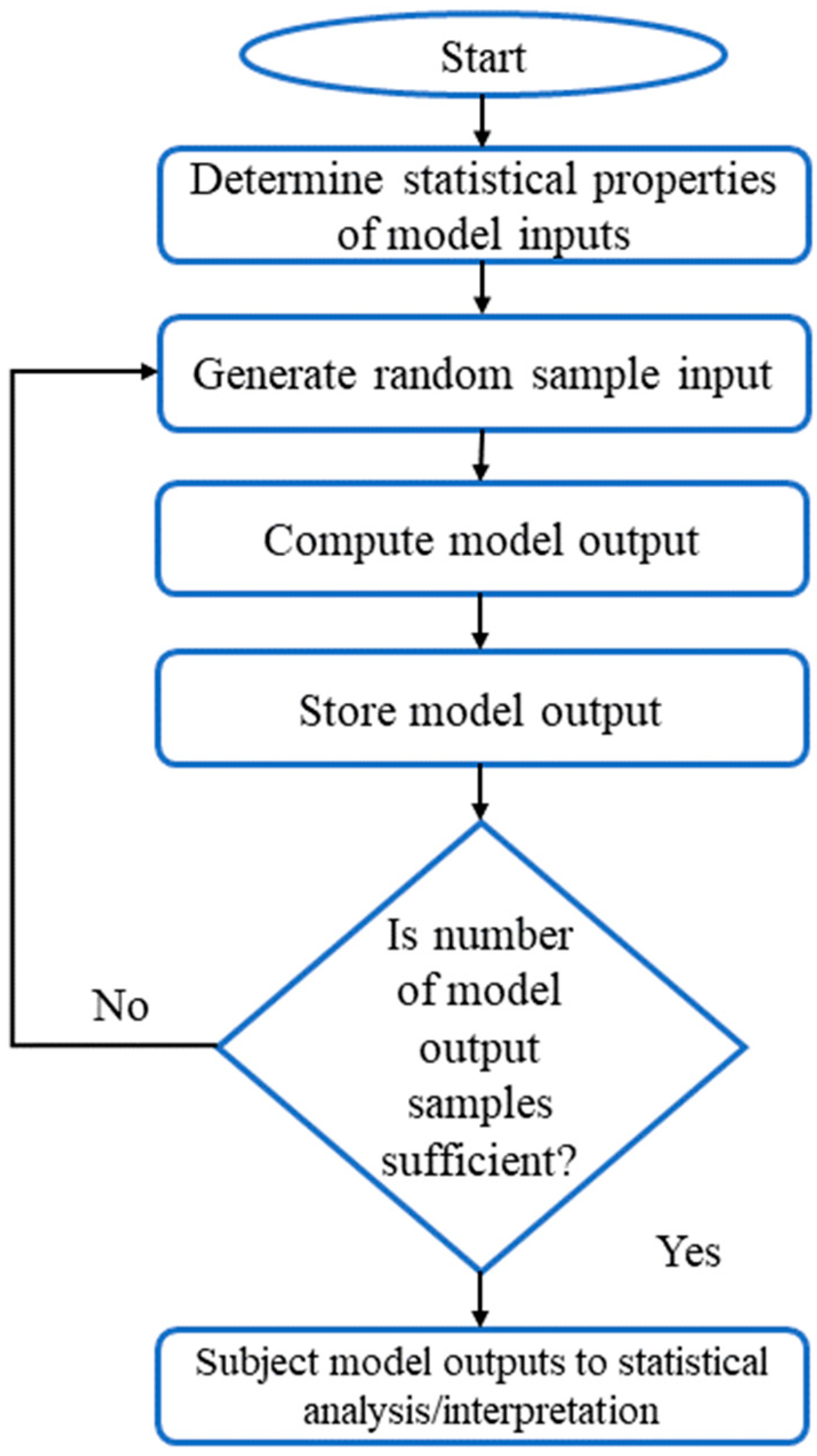
The MCS technique, formally introduced in 1949 [27], is the most widely used technique for determining the progression of uncertainties in random parameters. Indeed, this method can be used for any model. Moreover, the statistical results of MCS are realistic, so it is always used as a reference method. MCS is based on drawing N random samples from the probability density function of the random variables. Each realization constitutes a deterministic problem that must be solved through a deterministic method. To achieve good accuracy, the MCS technique requires many samples. Therefore, if the processing time of a single sample is very high, the methodology will become very expensive in terms of computational time. Consequently, its use in complex problems is avoided [27].

In this work, simulations by MCS have been performed following the description (Figure 2). It started with the identification of the uncertain parameters, then the random generation of these parameters in the model, and the calculation of their responses. Finally, the calculation of their mean value and standard deviation was performed. The execution of the simulation involving 100,000 Monte Carlo samples required approximately 48 h of computational time. The resulting dataset is utilized as a benchmark solution for validating the outcomes obtained via the Polynomial Chaos Expansion (PCE) technique. It is important to note that the Monte Carlo Simulation (MCS) method is characterized by slow convergence behavior and typically necessitates many realizations to achieve statistically significant results, with 100,000 samples being a common requirement.

4.2. Polynomial Chaos

This segment introduces a contemporary procedural framework grounded in the projection of principal components. The technique involves projecting targeted stochastic resolutions utilizing orthogonal polynomial functions with orthonormal Gaussian variables [28]. The foundational polynomial characteristics are leveraged to derive a linear equation system via solution projection, resulting in a polynomial basis expansion for the resolution. This expansion facilitates the computation of the probabilistic solution’s statistical moments. By implementing this methodology, the dynamic response of the mechanical system is numerically evaluated.

The generalization of the Polynomial Chaos method can be resolved into a series of convergent polynomial functions as follows:

$${\mathrm{V}}_{\mathrm{i}}\left(\mathrm{x},\mathsf{\xi }\right)={\sum }_{\mathrm{j}=0}^{\mathrm{\infty }}{\overline{\mathsf{\nu }}}_{\mathrm{ij}}{\mathsf{\varphi }}_{\mathrm{j}}\left(\mathsf{\xi }\right),\mathsf{\xi }=\left({\mathsf{\xi }}_1,{\mathsf{\xi }}_2, ...\right)$$

(21)

where x is the nodal displacement vector.

In which ${\mathsf{\varphi }}_{\mathrm{j}}\left(\mathsf{\xi }\right)$ denote an orthogonal polynomial within independent random factors $\mathsf{\xi }$ with a given random density of probability $\mathrm{W}\left(\mathsf{\xi }\right)$.

$$⟨{\mathsf{\varphi }}_{\mathrm{i}},{\mathsf{\varphi }}_{\mathrm{j}}⟩=\int {\mathsf{\varphi }}_{\mathrm{i}}{\mathsf{\varphi }}_{\mathrm{j}}\mathrm{W}\left(\mathsf{\xi }\right)\mathrm{d}\left(\mathsf{\xi }\right)=\left\{\begin{array}{c}0\\ ⟨{\mathsf{\varphi }}_{\mathrm{i}},{\mathsf{\varphi }}_{\mathrm{j}}⟩\end{array}\begin{array}{c}\mathrm{i}\mathrm{f} \mathrm{i}\ne j\\ \mathrm{i}\mathrm{f} \mathrm{i}=\mathrm{j}\end{array}\right.$$

(22)

According to Askey’s scheme, Legendre polynomials are the most relevant for treating uncertainties. The order of the Polynomial Chaos method is given by:

$${\mathrm{N}}_{\mathrm{p}}={\displaystyle \frac{\left(\mathrm{p}+\mathrm{r}\right)!}{\mathrm{P}!\mathrm{r}!}}-1$$

(23)

To determine the coefficients ${\overline{\mathrm{V}}}_{\mathrm{ij}}$, the non-intrusive approach was used. This approach is particularly efficient, since it only requires simulations performed on specific models of the random variables [29]. It consists of reducing the minimum of the gap $\epsilon$ produced through the solution of the random model and its approximation in the generalized Polynomial Chaos basis.

$$\mathsf{\epsilon }={\sum }_{\mathrm{k}=1}^{\mathrm{Q}}\left[{\mathrm{V}}_{\mathrm{i}}\left(\mathrm{x},{\mathsf{\xi }}^{\left(\mathrm{k}\right)}\right)-{\sum }_{\mathrm{j}=0}^{\mathrm{N}\mathrm{p}}{\overline{\mathrm{V}}}_{\mathrm{i}\mathrm{j}}\left(\mathrm{x}\right){\mathrm{f}}_{\mathrm{j}}\left({\mathsf{\xi }}^{\left(\mathrm{k}\right)}\right)\right]$$

(24)

In efforts to minimize vibrational amplitudes within the transmission mechanism, prior studies have demonstrated that the dynamic response of the system is influenced by a multitude of mechano-geometric parameters. These factors introduce variability that can stem from various sources, including inherent design and manufacturing tolerances, as well as external perturbations arising from environmental interactions. Moreover, during the system design phase, many parameters must be assigned uncertainty intervals to account for stochastic variations. This raises critical questions regarding the system’s dynamic displacement, dimensional stability, and operational longevity, as well as the validity of the defined uncertainty bounds. Specifically, it remains an open challenge whether a single uncertainty interval can sufficiently capture the dynamic behavior of a system governed by multiple interdependent uncertain parameters.

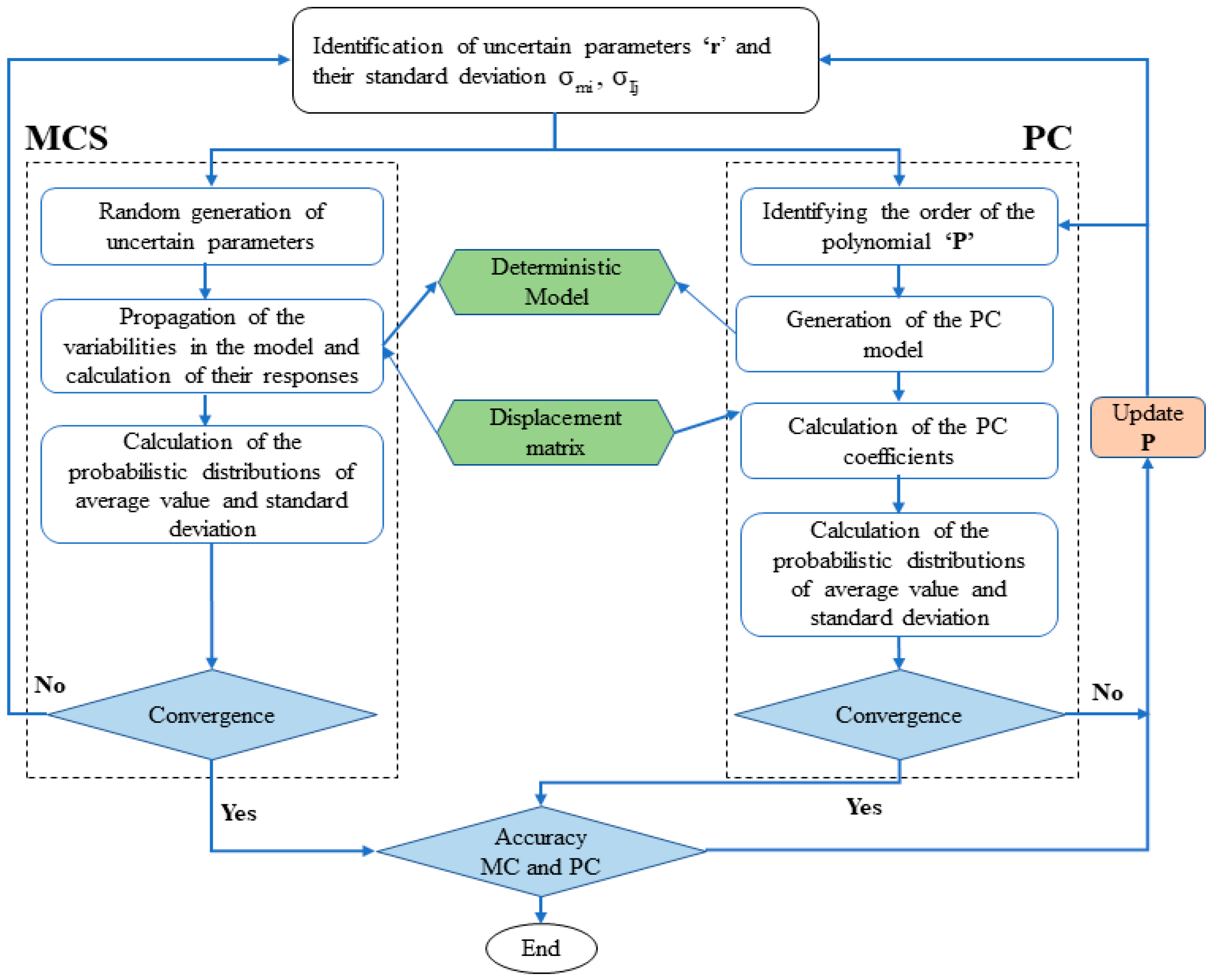
In the coming section, the physical parameters of mass, moment of inertia, the bearing’s bending stiffness, the traction-compression stiffness, the damping coefficient, and the wind speeds for the two-stage gearbox will be defined as random variables using Monte Carlo and Polynomial Chaos methods according to a procedure described in the flowchart of the numerical model in Figure 3. This study will allow us to examine the standard deviation of these parameters considering multivariate uncertainty.

5. Numerical Simulation

The numerical simulation process in MATLAB R2025b initiates with the assembly of displacement matrices corresponding to the degrees of freedom defined in Equation (21). To account for parametric uncertainties, variations in mass, moment of inertia, bearing bending stiffness, traction-compression stiffness, damping coefficients, and wind speeds are incorporated into the model. These stochastic parameters are then processed using the Polynomial Chaos Expansion (PCE) methodology, which reconstructs the matrices by leveraging their mean values and prescribed standard deviations. This approach enables a probabilistic representation of the system’s response, ensuring robustness against the inherent variability of the input parameters.

The numerical simulation in this study is a combination of two approaches, which are presented in a coupled form (Figure 3). The simulation begins with identifying the uncertain parameters and their standard deviation. The MCS is then performed in three main steps: randomly generating uncertain parameters, propagating them through the model to calculate responses using a deterministic model, and finally calculating their mean value and standard deviation. Once the MCS is complete, the PC calculation begins with three main steps: generating the model, calculating the polynomial coefficients of the chaos, and calculating the probabilistic distribution of the mean values and standard deviations. The two approaches converge, and the results are compared.

As part of this study, the different system parameters used in the simulation are presented in

Table 1. System parameters used in the simulation.

Torque	100 N.m
Bearing stiffness	$k_j^x$ = 5 × 108 N/m  $k_j^y$ = 5 × 108 N/m
Shaft torsional stiffness	$k_j^{\theta }$ = 106 Nm/rad
Number of teeth of the first gear	${\mathrm{Z}}_{12}=63,{\mathrm{Z}}_{21}=20$
Number of teeth of the second gear	${\mathrm{Z}}_{22}=65,{\mathrm{Z}}_{31}=12$
Teeth modulus	${\mathrm{m}}_1={\mathrm{m}}_2=14.10^{-3} \mathrm{m}$
Contact ratio	${\mathsf{\epsilon }}_{\mathsf{\alpha }1}=1.734,{\mathsf{\epsilon }}_{\mathsf{\alpha }2}=1.733$
Pressure angle	${\mathsf{\alpha }}_1={\mathsf{\alpha }}_2=20 °$
Moment inertia of the rotor	$2587 \mathrm{k}\mathrm{g}·{\mathrm{m}}^2$
Generator velocity	$1500 \mathrm{r}\mathrm{p}\mathrm{m}$
Teeth width	${\mathrm{b}}_1={\mathrm{b}}_2=0.1 \mathrm{m}$
Power coefficient	${\mathrm{C}}_{\mathrm{p}}=44\%$
Air density	$\mathsf{\rho }=1.225 \mathrm{k}\mathrm{g}/{\mathrm{m}}^3$
Rotor radius	$\mathrm{R}=6 \mathrm{m}$
Basic radius of wheels	${\mathrm{r}}_{12}^b=0.8 \mathrm{m},r_{21}^b=0.2 \mathrm{m},r_{22}^b=0.5 \mathrm{m},r_{31}^b=0.1 \mathrm{m}$

.

In the following simulations, uncertainty approaches are implemented to analyze the dynamic behavior of the system in the presence of uncertainties in the design parameters. A case study of coupled forms was analyzed to evaluate the effect of such uncertainty on the dynamic response of a two-stage gear transmission using the mentioned approaches (Figure 3). The dynamic response of the first bearing is studied along both the x and y axes. The simulation parameters used are shown in Table 1. The numerical results obtained through the PC methodology are evaluated and validated against an MCS comparison comprising up to 100,000 simulations.

The random variables considered below are: the mass of the gear wheels ${\mathrm{m}}_{\mathrm{g}}$, the damping coefficients $\mathsf{\eta }=10^{-2}$, $\mathsf{\mu }=10^{-5}$, the inertia of the wheel ${\mathrm{I}}_{\mathrm{w}}$, the inertia of the pinion ${\mathrm{I}}_{\mathrm{p}}$, and the driving inertia ${\mathrm{I}}_{\mathrm{m}}$.

$${\mathrm{m}}_{\mathrm{g}}={\mathrm{m}}_{\mathrm{g},0}+{\mathsf{\sigma }}_{{\mathrm{m}}_{\mathrm{g}}}\mathsf{\xi }$$

(25)

$$\mathsf{\eta }={\mathsf{\eta }}_0+{\mathsf{\sigma }}_{\mathsf{\eta }}\mathsf{\xi }$$

(26)

$$\mathsf{\mu }={\mathsf{\mu }}_0+{\mathsf{\sigma }}_{\mathsf{\mu }}\mathsf{\xi }$$

(27)

$${\mathrm{I}}_{\mathrm{w}}={\mathrm{I}}_{\mathrm{w},0}+{\mathsf{\sigma }}_{{\mathrm{I}}_{\mathrm{w}}}\mathsf{\xi }$$

(28)

$${\mathrm{I}}_{\mathrm{P}}={\mathrm{I}}_{\mathrm{P},0}+{\mathsf{\sigma }}_{{\mathrm{I}}_{\mathrm{P}}}\mathsf{\xi }$$

(29)

$${\mathrm{I}}_{\mathrm{d}}={\mathrm{I}}_{\mathrm{d}}+{\mathsf{\sigma }}_{{\mathrm{I}}_{\mathrm{d}}}\mathsf{\xi }$$

(30)

where $\mathsf{\xi }$ represents the Gaussian random variable with zero mean; ${\mathrm{m}}_{\mathrm{g},0}$, ${\mathrm{I}}_{\mathrm{w},0}$, ${\mathrm{I}}_{\mathrm{P},0}$, ${\mathsf{\eta }}_0$, ${\mathsf{\mu }}_0$, ${\mathrm{I}}_{\mathrm{d},0}$ denotes the mean value, respectively. ${\mathsf{\sigma }}_{{\mathrm{m}}_{\mathrm{g}}}$, ${\mathsf{\sigma }}_{{\mathrm{I}}_{\mathrm{d}}}$, ${\mathsf{\sigma }}_{\mathsf{\eta }}$, ${\mathsf{\sigma }}_{\mathsf{\mu }}$, ${\mathsf{\sigma }}_{{\mathrm{I}}_{\mathrm{p}}}$, ${\mathsf{\sigma }}_{{\mathrm{I}}_{\mathrm{w}}}$ are the standard deviations of these parameters.

To evaluate the effect of the standard deviation and the dynamic response of the studied system, the standard deviations used in the simulations are $\mathsf{\sigma } = 2\%$.

6. Results

6.1. Impact of Uncertain Gear Mass

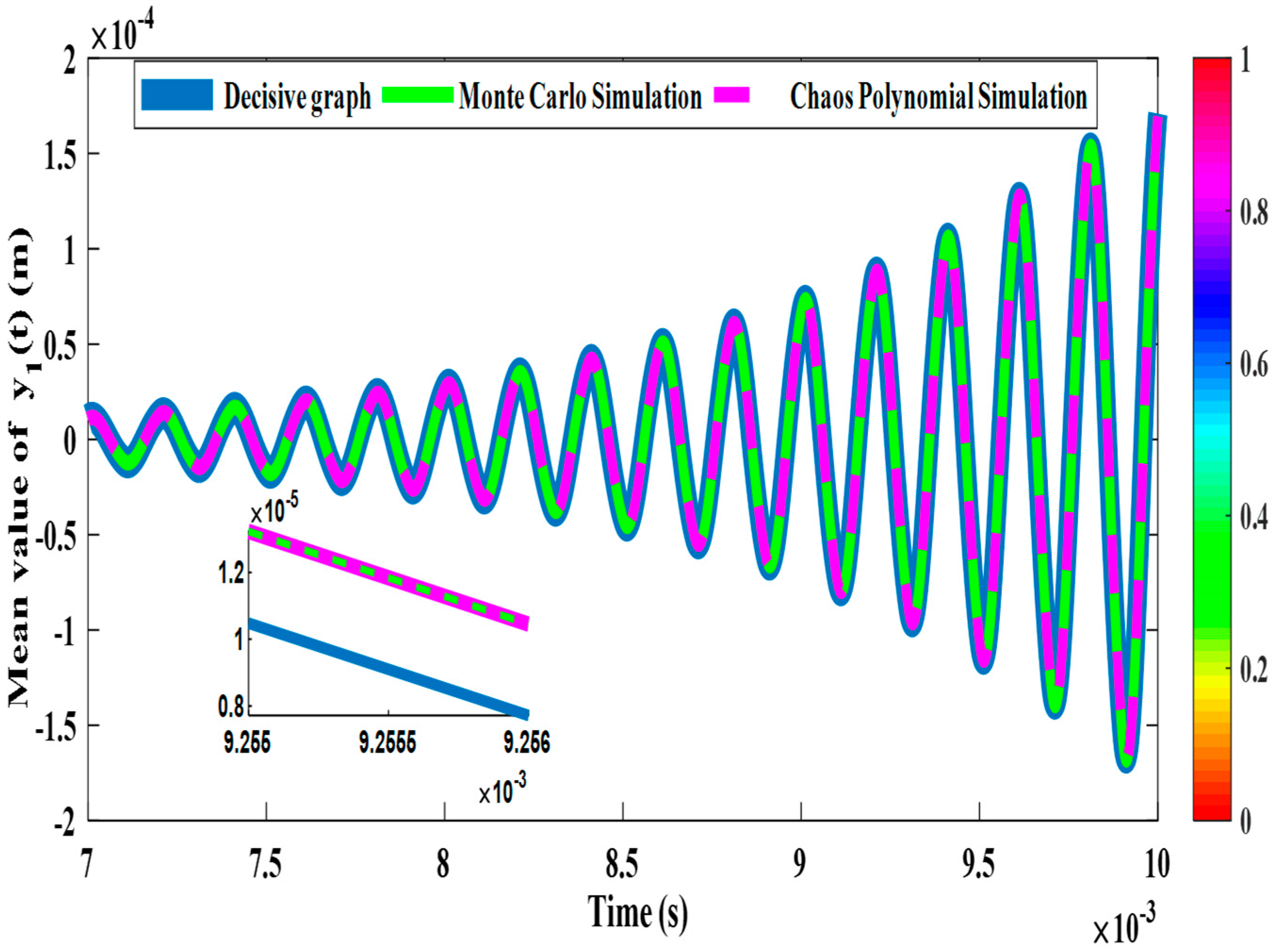
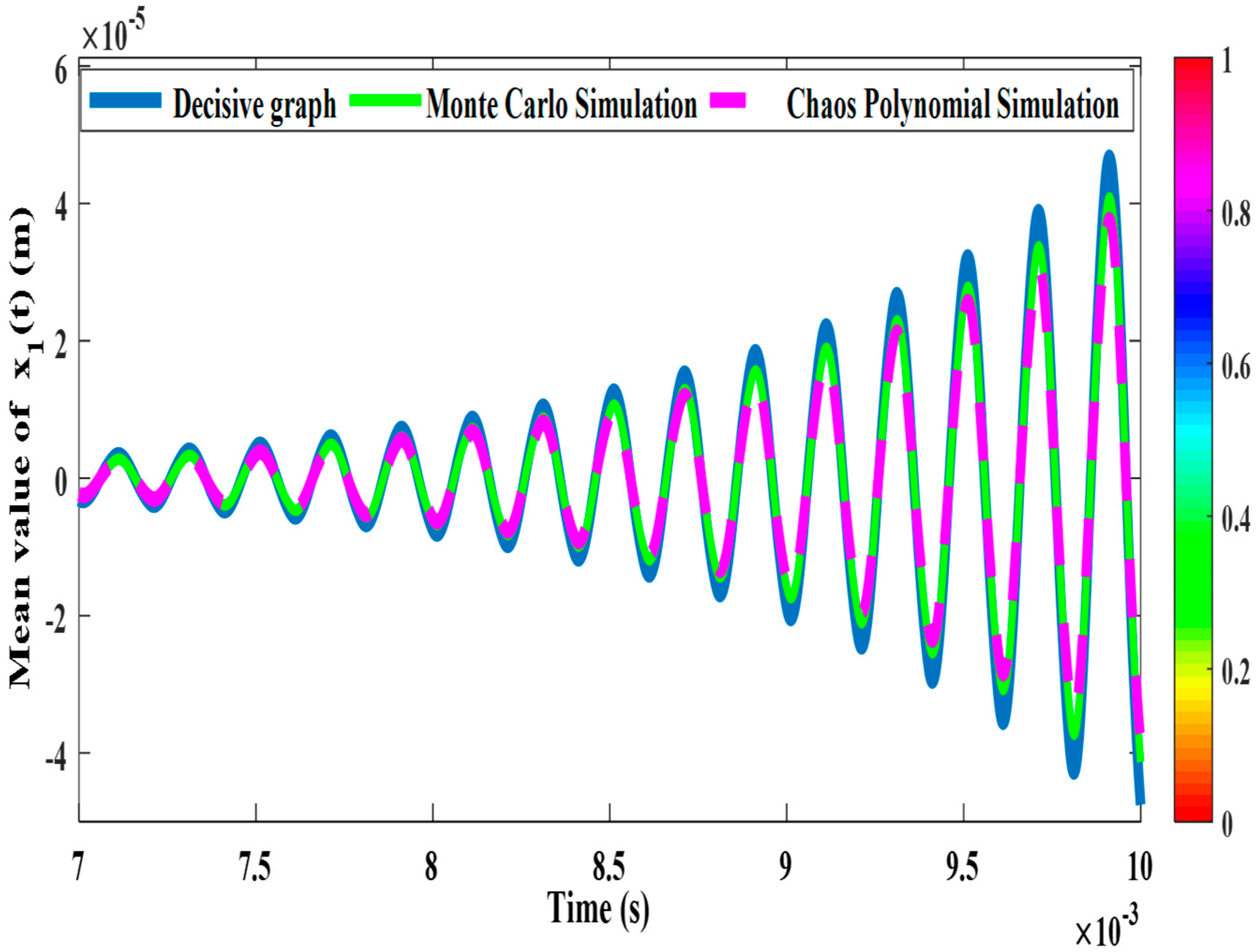
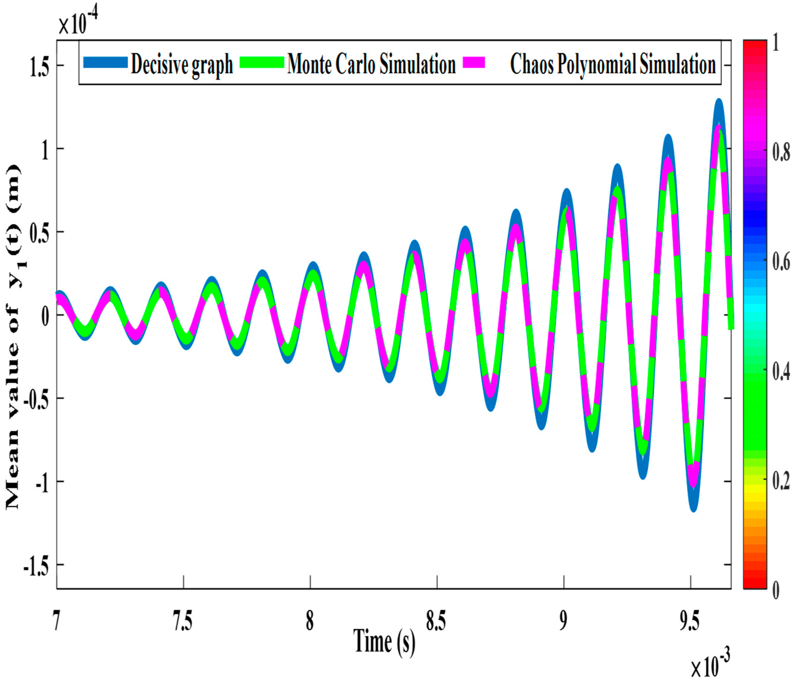
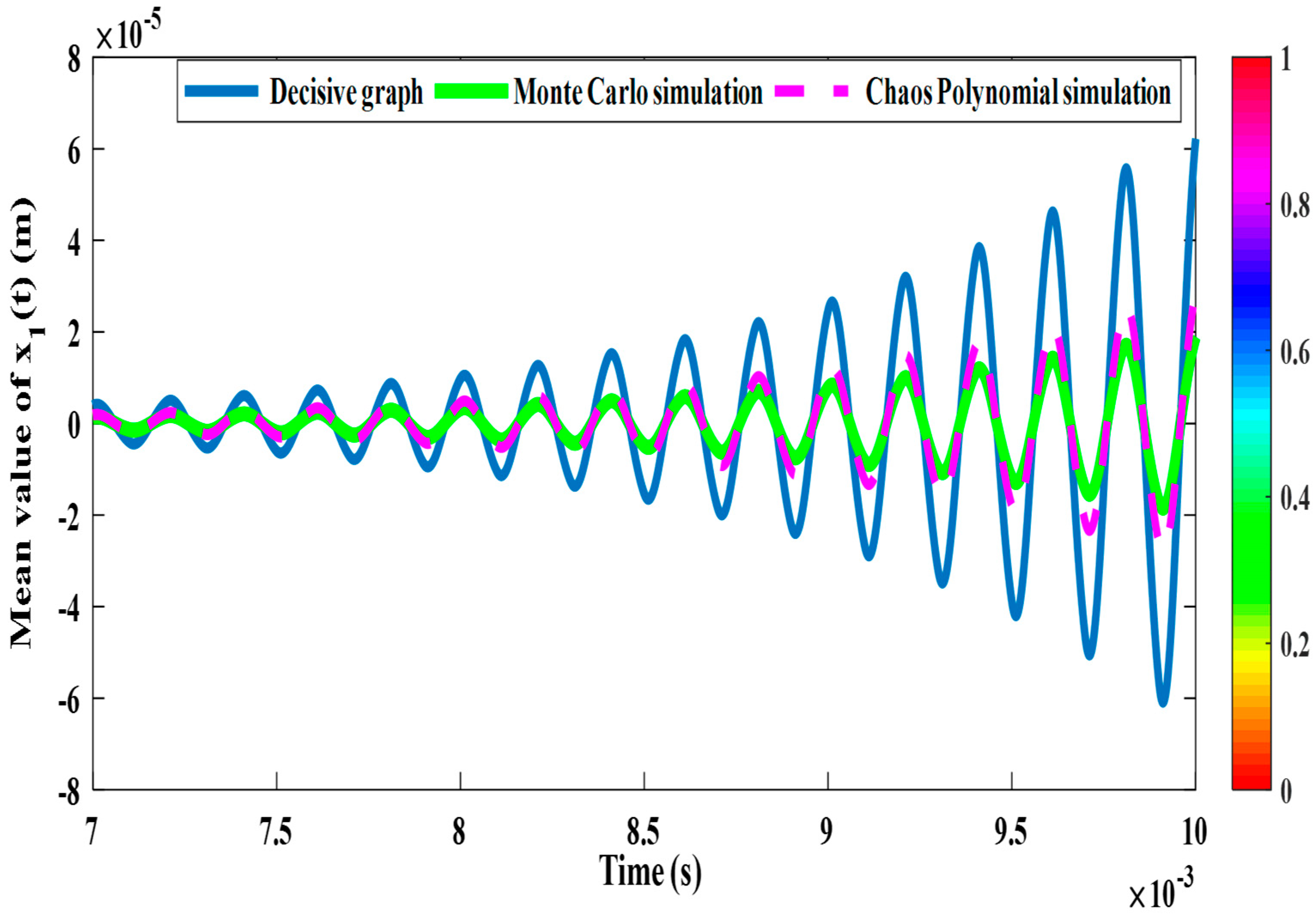
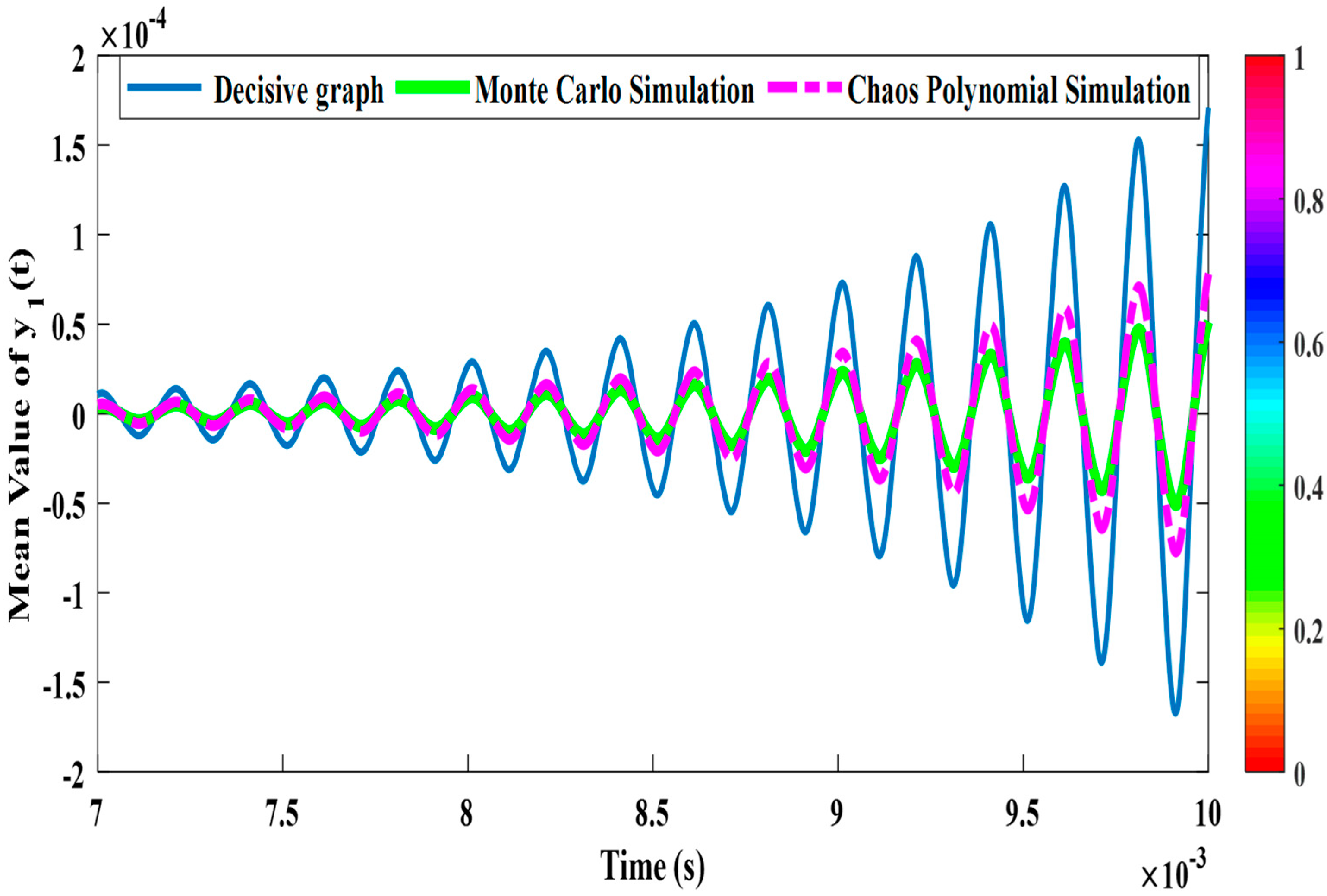
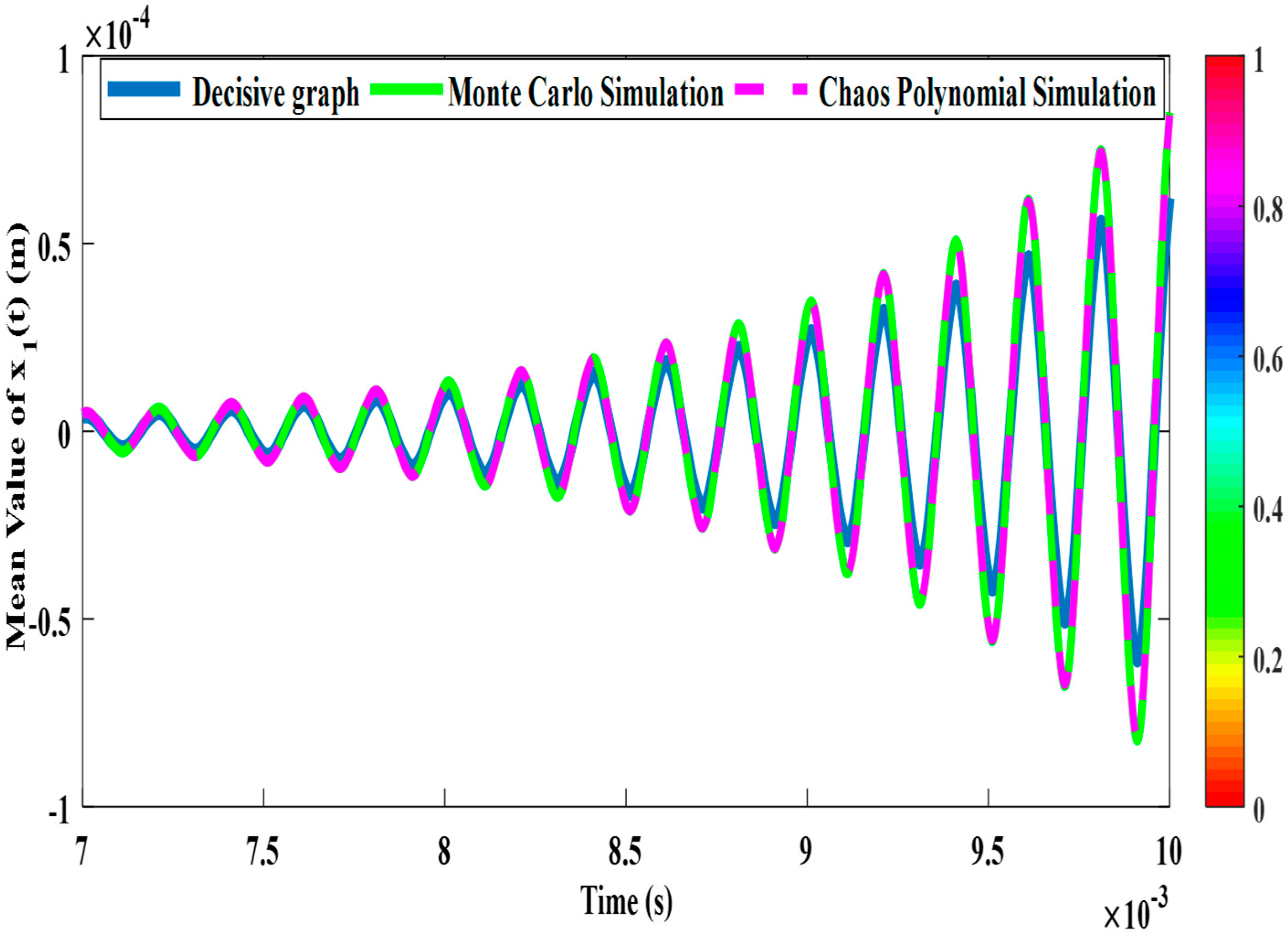
Figure 4 and Figure 5 show the mean values of the linear displacement along the x and y axes, represented by three curves: the deterministic graph, the MCS response, and the mean value of the PC simulation. When incorporating mass uncertainty into the simulation, it should be noted that the average values of ${\mathrm{x}}_1\left(\mathrm{t}\right)$ and ${\mathrm{y}}_1\left(\mathrm{t}\right)$ remain relatively stable, with the MCS and PC curves closely following the deterministic solution, suggesting a limited influence of uncertainties on the mean value.

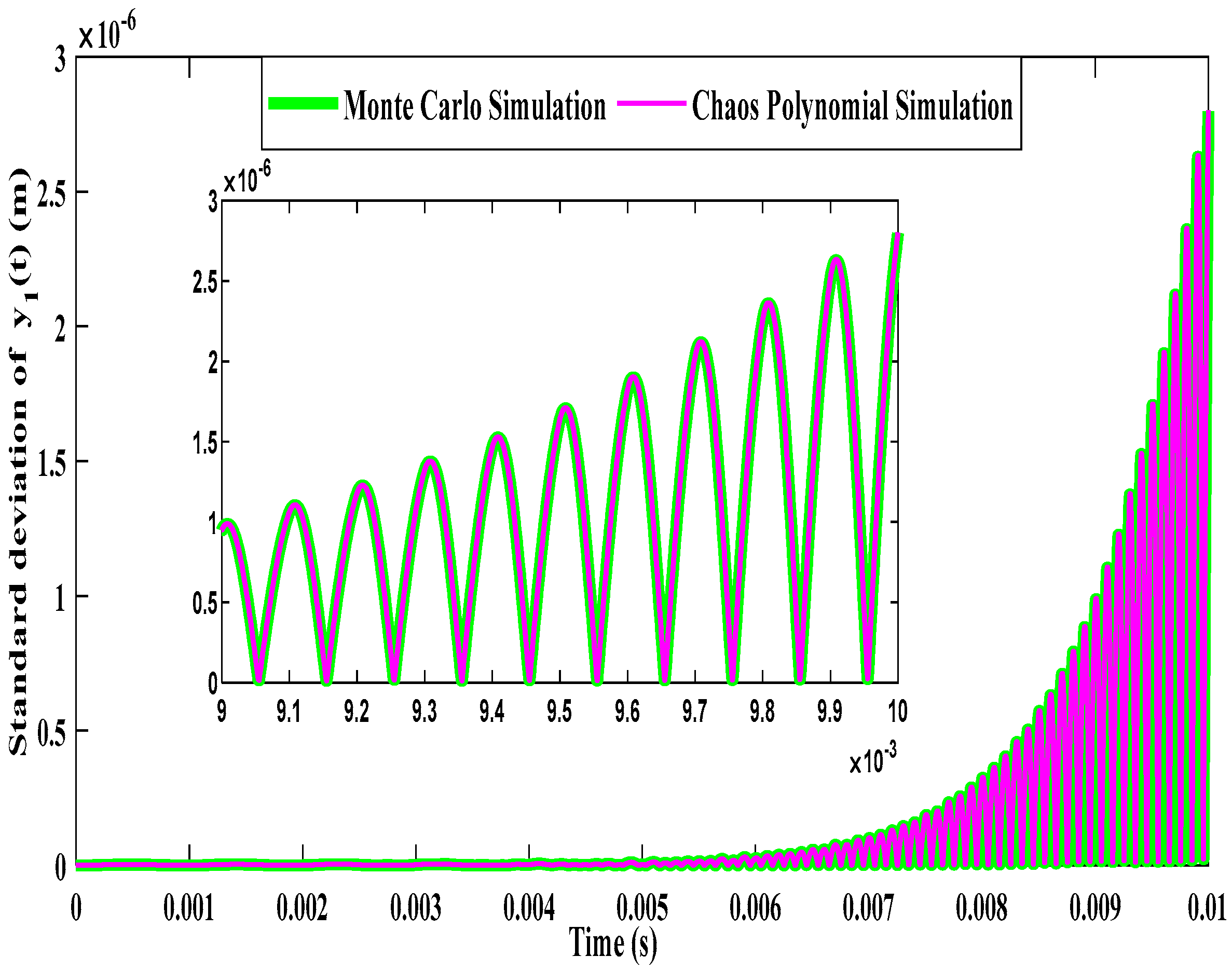
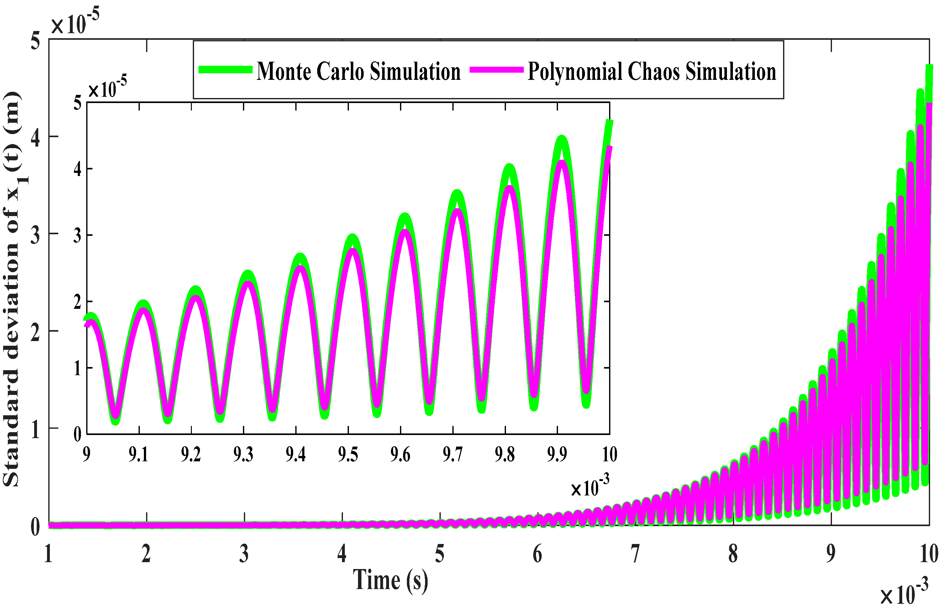
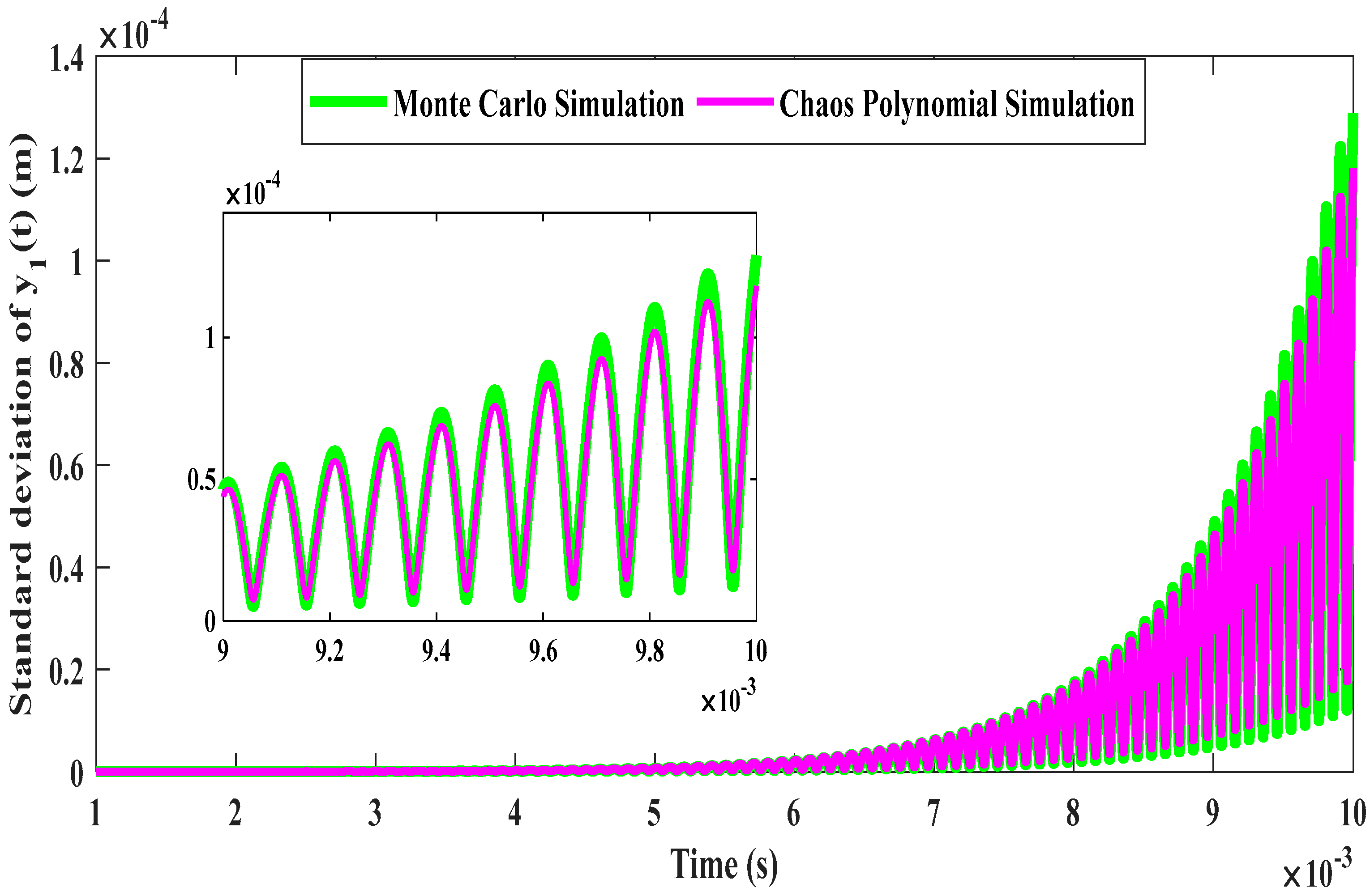
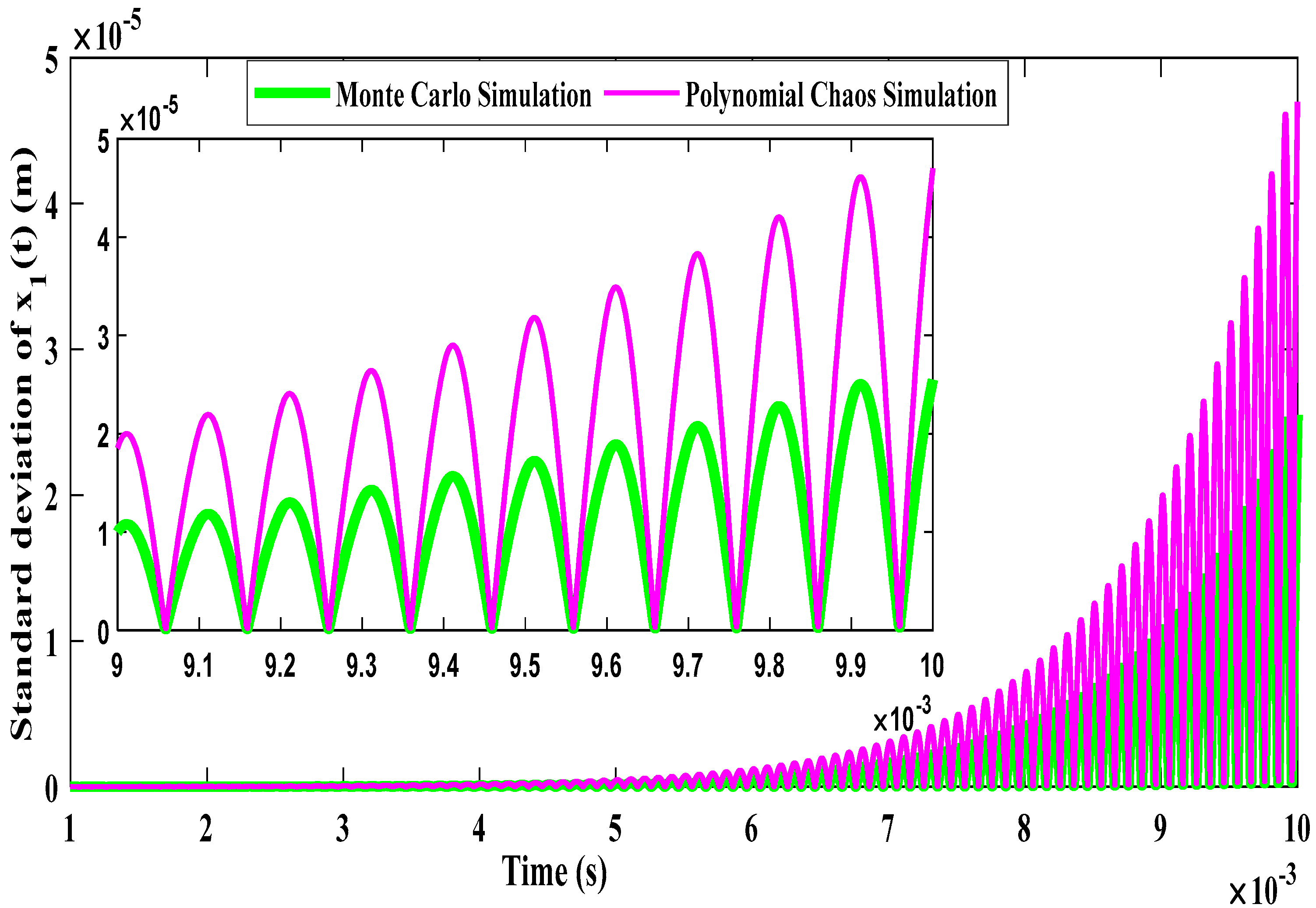
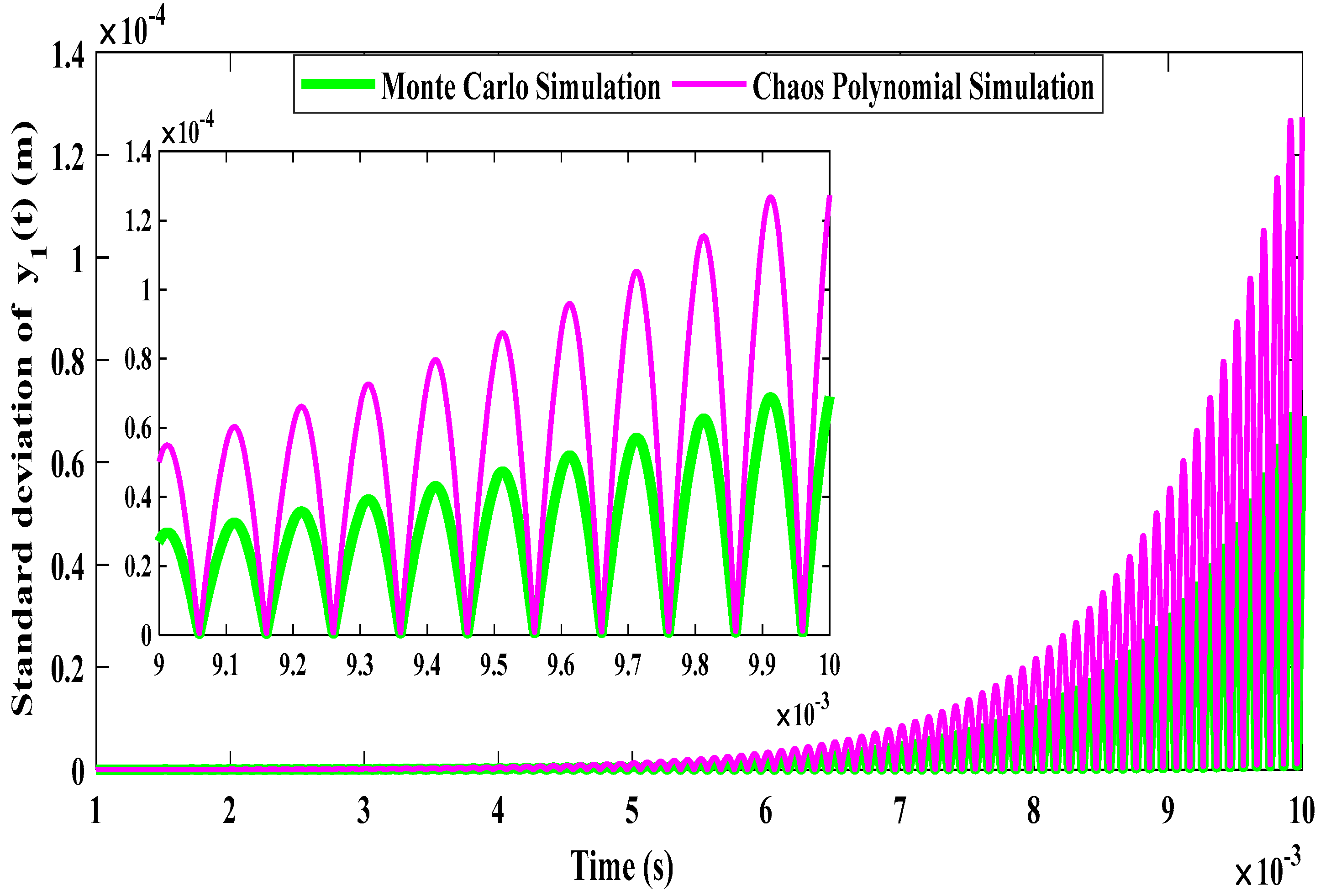
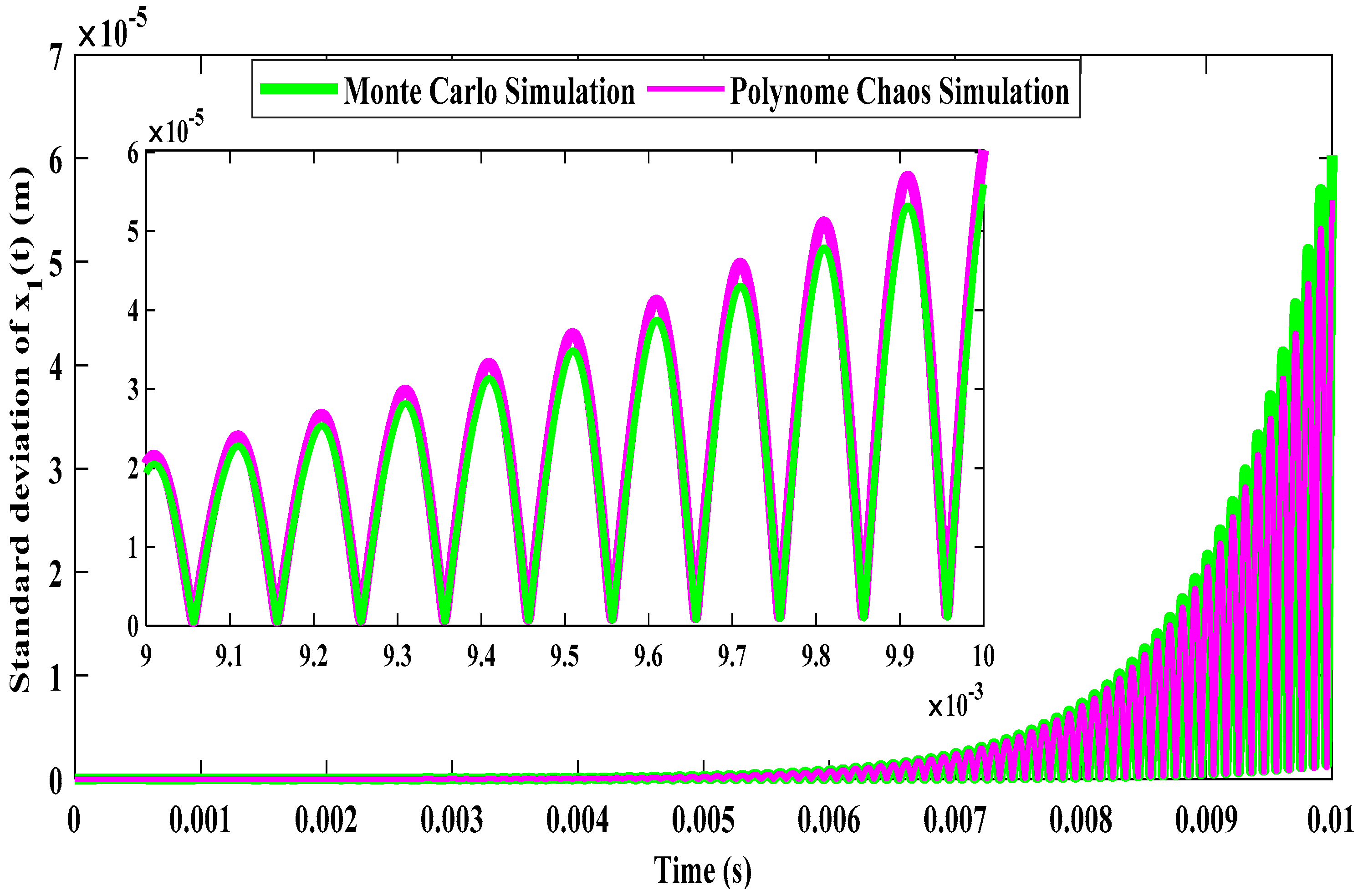
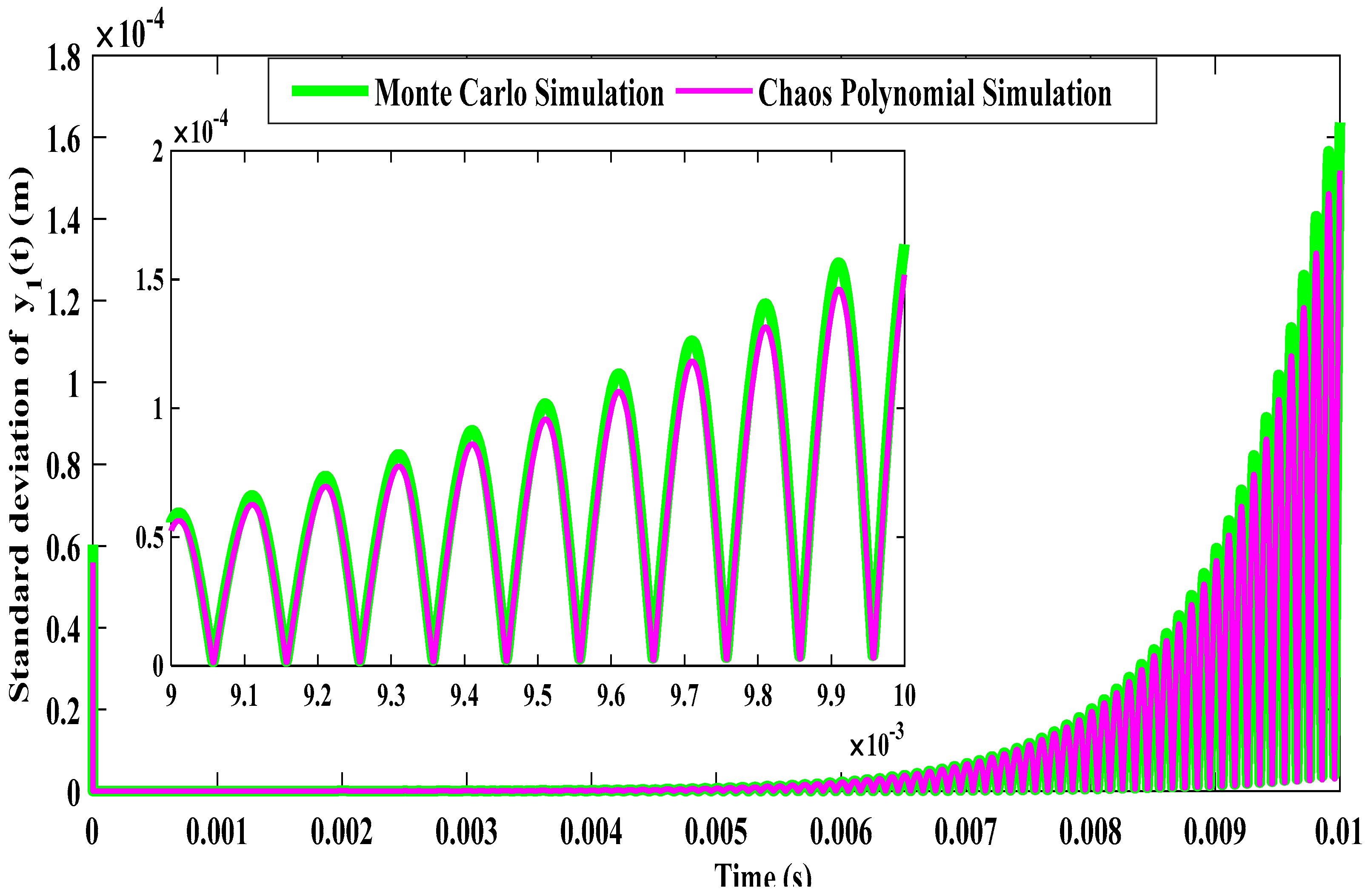
According to the values given by the standard deviation (Figure 6 and Figure 7), the influence of the uncertain variable is more pronounced on ${\mathrm{y}}_1\left(\mathrm{t}\right)$ than on ${\mathrm{x}}_1\left(\mathrm{t}\right)$. For ${\mathrm{x}}_1\left(\mathrm{t}\right)$, the standard deviation gradually increases to about $5\times {10}^{-5}$, indicating moderate variability due to uncertainties. In contrast, for ${\mathrm{y}}_1\left(\mathrm{t}\right)$, the standard deviation reaches approximately $1.4\times {10}^{-5}$, showing much greater variability and a more significant influence of uncertainties.

6.2. Impact of Damping Coefficient

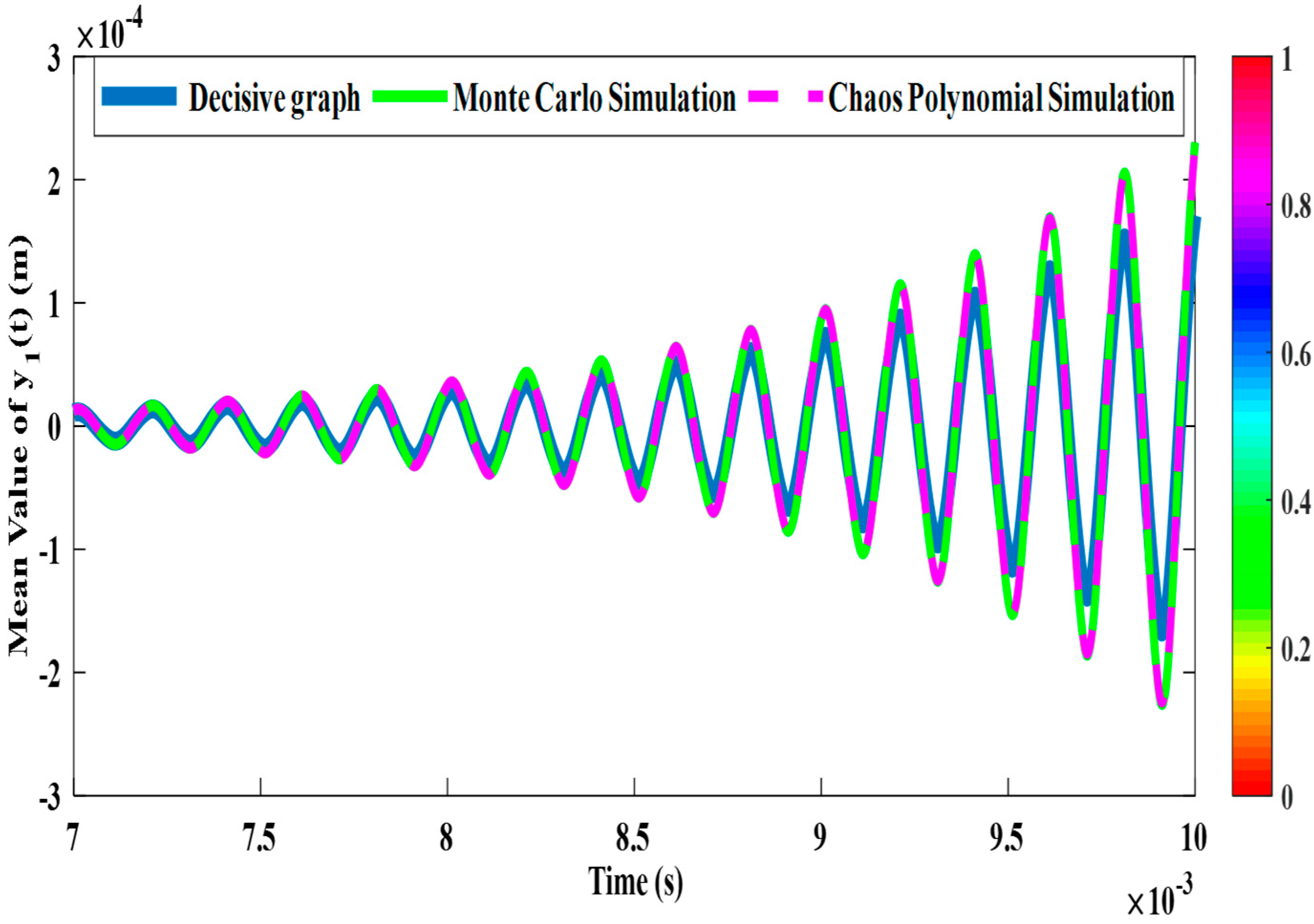
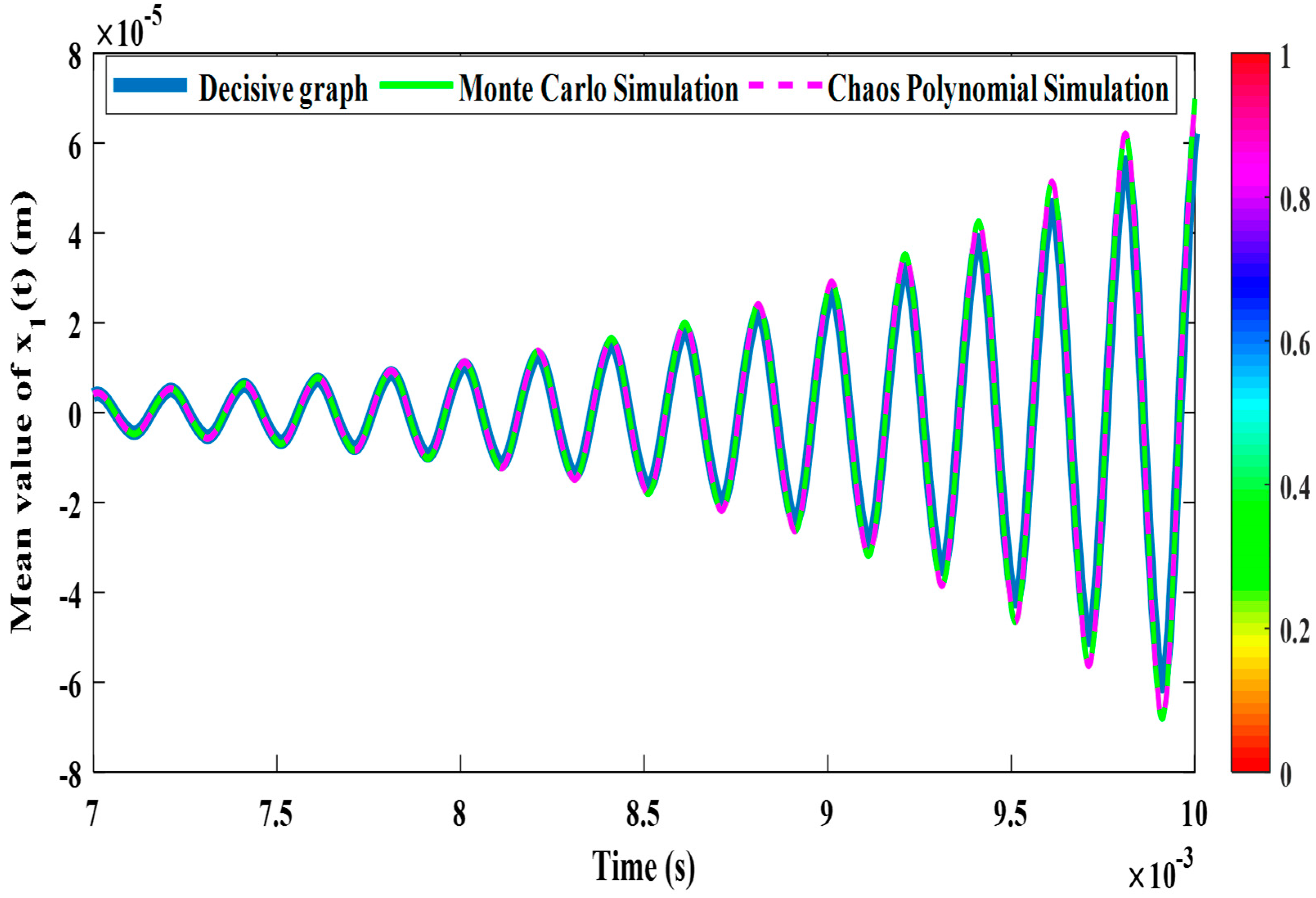
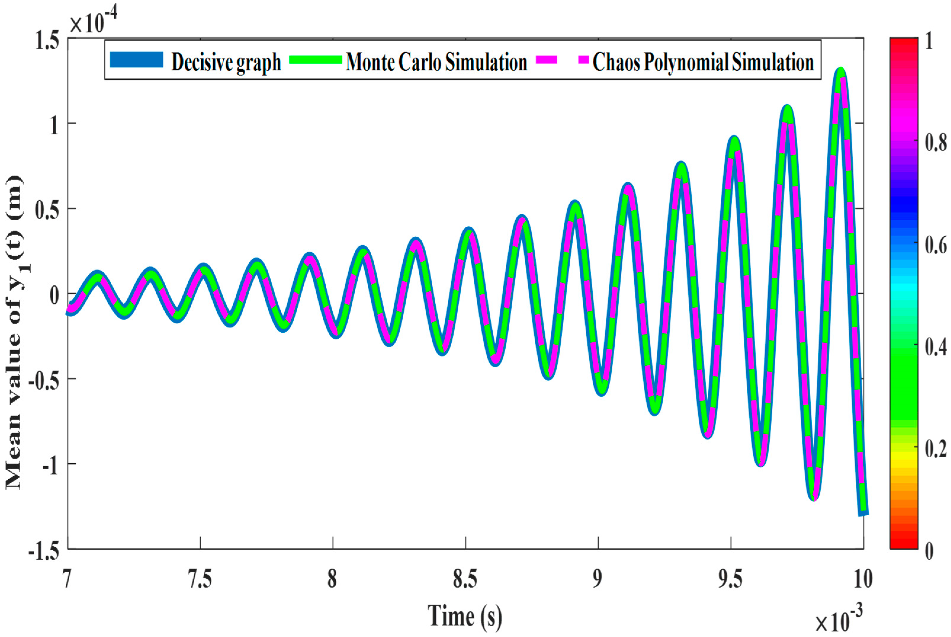
The comparison between the deterministic solution and the two other simulations (Monte Carlo and Polynomial Chaos) (Figure 8 and Figure 9) shows that, despite the uncertainty in the damping coefficients, both methods effectively reproduce the overall trend of the deterministic solution. The simulation curves exhibit a slight attenuation of the oscillations, indicating that the uncertainty in the damping coefficients primarily impacts local variations (peaks and troughs) without significantly affecting the overall mean value. In summary, while the uncertainty in the coefficients slightly reduces the precision of the oscillations, it does not alter the mean value of the system’s response.

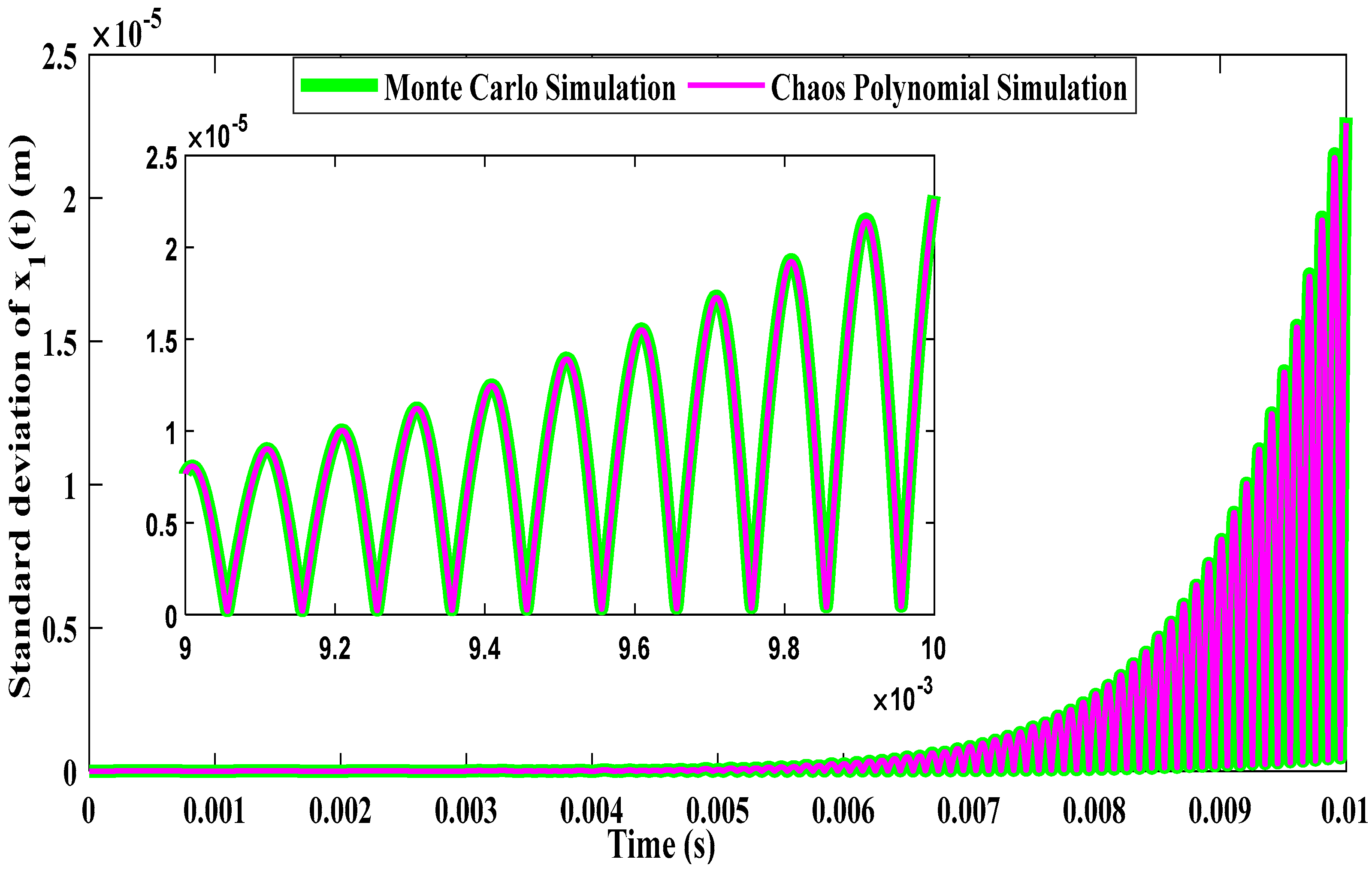
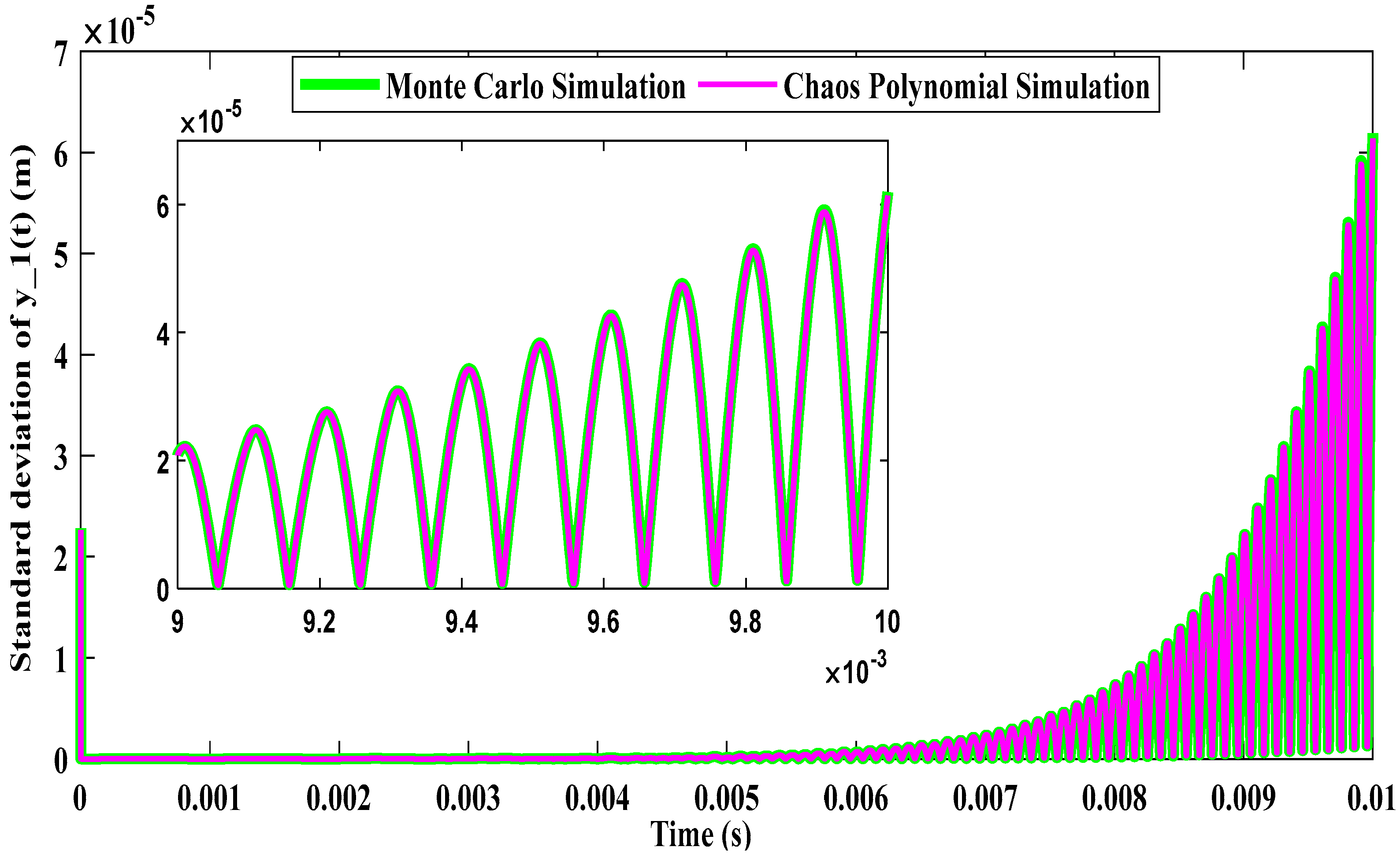
According to the values given by the standard deviation (Figure 10 and Figure 11), the influence of the uncertain variable is more pronounced on ${\mathrm{y}}_1\left(\mathrm{t}\right)$ than on ${\mathrm{x}}_1\left(\mathrm{t}\right)$. For displacement along the x-axis, the standard deviation gradually increases up to approximately $5\times {10}^{-5}$, indicating moderate variability. In contrast, along the y-axis, the standard deviation reaches about $1.4\times {10}^{-4}$, showing much greater variability and a significant influence of uncertainties.

6.3. Impact of the Pinion’s Moment of Inertia

Figure 12 and Figure 13 show the mean values of the linear displacement along the x-axis and the y-axis that are presented by three curves: the deterministic solution, the response of the MCSs, and the mean value of the PC simulation with ${\mathsf{\sigma }}_{\mathrm{m}} = 2\%$. By exploiting an uncertain mass in the simulation, it should be noted that the average values of ${\mathrm{x}}_1\left(\mathrm{t}\right)$ and ${\mathrm{y}}_1\left(\mathrm{t}\right)$ remain relatively stable, with the MCS and PC curves closely following the deterministic solution, suggesting a limited influence of uncertainties on the mean value.

In the case where the pinion’s moment of inertia is considered uncertain, the results are presented in Figure 14 and Figure 15. These results show equal values, $3\times 10^{-6}$, in terms of standard deviation levels. This would imply that the effect due to the uncertainty of the pinion’s moment of inertia is evenly distributed between the two axes. Such a situation would indicate that this uncertainty similarly affects displacements along both the x and y axes.

6.4. Impact of the Wheel’s Uncertain Inertia

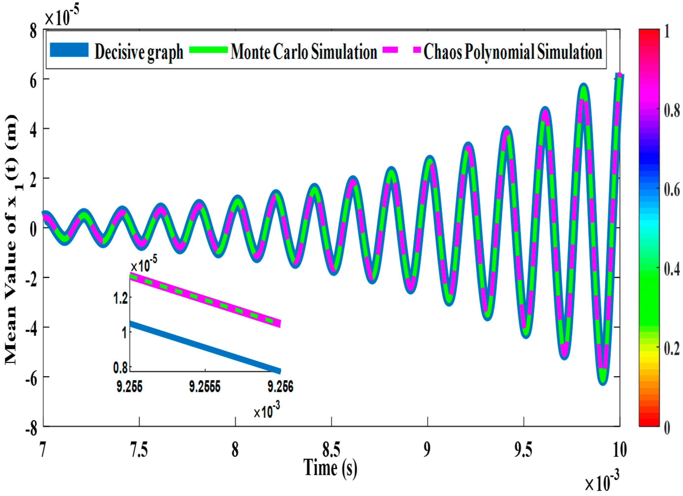
By comparing the curves (Figure 16 and Figure 17), it is evident that the uncertainty in the wheel inertia has a more significant impact on the mean displacement values along the x-axis compared to the y-axis. This effect is visible through the amplitude of oscillation and the dispersion of results, particularly in the Monte Carlo Simulation and the Polynomial Chaos simulation.

According to the values given by the standard deviation (Figure 18 and Figure 19), the influence of the uncertain variable is more pronounced on ${\mathrm{y}}_1\left(\mathrm{t}\right)$ than on ${\mathrm{x}}_1\left(\mathrm{t}\right)$. For displacement along the x-axis, the standard deviation gradually increases up to approximately $7\times 10^{-5}$, indicating moderate variability. In contrast, along the y-axis, the standard deviation reaches about $1.8\times 10^{-4}$, showing much greater variability and a significant influence of uncertainties.

6.5. Impact of Uncertain Driving Inertia

Figure 20 and Figure 21 show the mean values of the linear displacement along the x-axis and the y-axis that are presented by three curves: the deterministic solution, the response of the MCSs, and the mean value of the PC simulation with ${\mathsf{\sigma }}_{{\mathrm{I}}_{\mathrm{d}}} = 2\%$. By exploiting an uncertain mass in the simulation, it should be noted that the average values of ${\mathrm{x}}_1\left(\mathrm{t}\right)$ and ${\mathrm{y}}_1\left(\mathrm{t}\right)$ remain relatively stable, with the MCS and PC curves closely following the deterministic solution, suggesting a limited influence of uncertainties on the mean value.

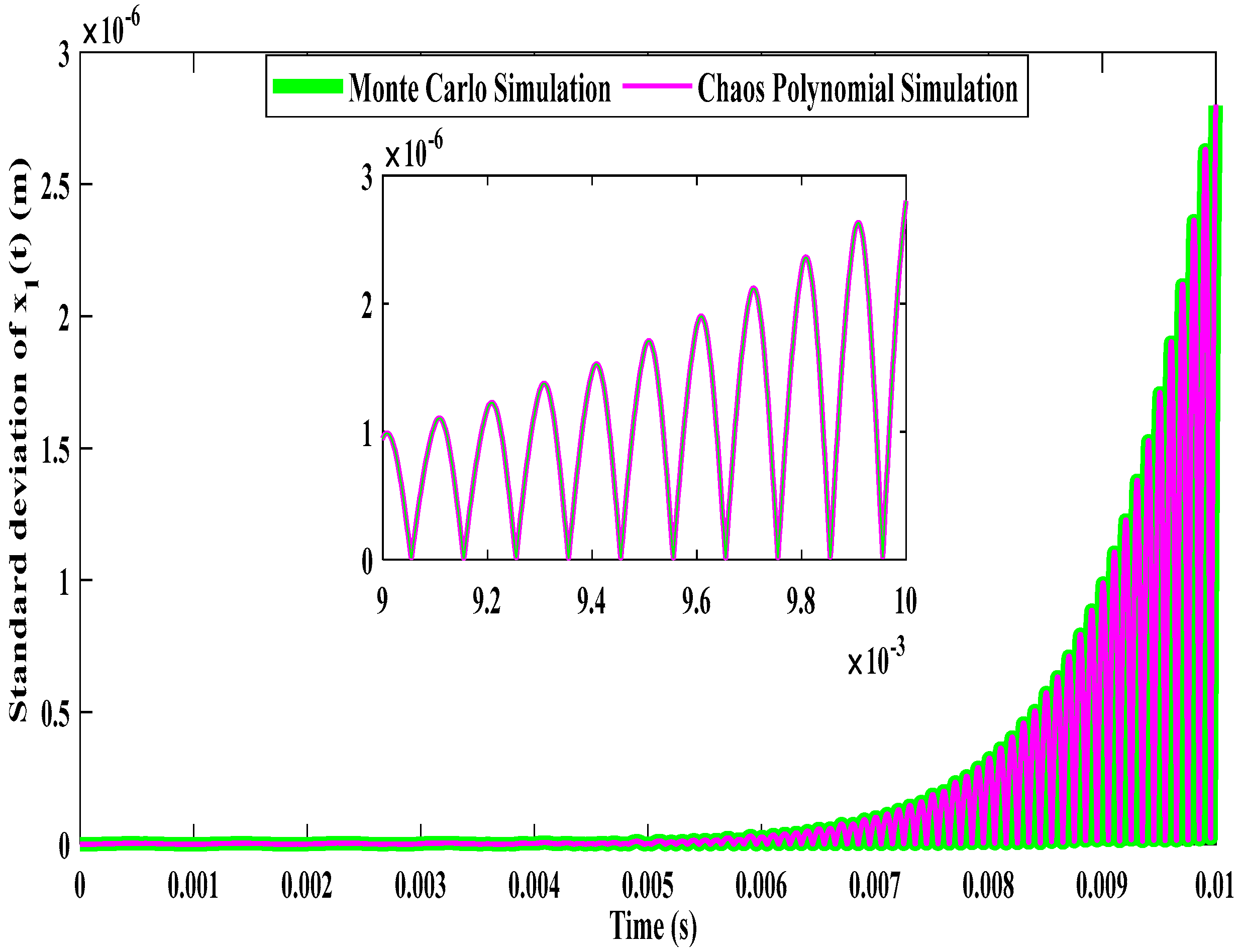
According to the values given by the standard deviation (Figure 22 and Figure 23), the influence of the uncertain variable is more pronounced on ${\mathrm{y}}_1\left(\mathrm{t}\right)$ than on ${\mathrm{x}}_1\left(\mathrm{t}\right)$. For displacement along the x-axis, the standard deviation gradually increases up to approximately $2.5\times 10^{-5}$, indicating moderate variability. In contrast, along the y-axis, the standard deviation reaches about $7\times 10^{-5}$, showing much greater variability and a significant influence of uncertainties.

Table 2. Summary of the impact of uncertain parameters on the two directions.

Uncertain Parameters	Uncertainty Type	Impact on	Comments
Mass of gear wheels	Random	$x_1$: Low $y_1$: High $x_2$: low $y_2$: High	Significant effect on direction y
Damping coefficients	Random	$x_1$: strong $y_1$: strong $x_2$: weak $y_2$: average	More significant influence on the first two $\mathrm{Degrees} \mathrm{of} \mathrm{Freedom} (x_1$ and $y_1$)
Pinion inertia	Random	$x_1$: weak $y_1$: weak	Weak influence on both directions
Wheel inertia	Random	$x_1$: strong $y_1$: strong	Significant influence on both directions
Drive inertia	Random	$x_1$: weak $y_1$: strong	Weak influence along (x) and strong along (y)

evaluates the impact of uncertainties on the system, where the randomness of each parameter affects the system’s dynamic behavior along the (x) and (y) directions. The mass of the gearwheels has a significant effect on the (y) direction, likely influencing the alignment or vibration of the gears. The damping coefficients strongly impact the first two degrees of freedom ($x_1$ and $y_1$), which could relate to the primary stage of the gear system. The pinion inertia, representing the smaller gear, has a weak influence on both directions, while the wheel inertia, associated with the larger gear, has a strong impact on both (x) and (y). The drive inertia, linked to the input shaft, has a weak effect on the (x) direction but a strong effect on the (y) direction, potentially affecting the system’s torsional stability. These insights are critical for optimizing the performance and reliability of the two-stage gear system, particularly in applications requiring precise motion control and minimal vibration.

The Monte Carlo method estimates statistical properties by repeatedly evaluating a model with randomly sampled inputs, making it simple, non-intrusive, and applicable to a wide range of problems. However, its computational cost is often very high because the convergence rate is slow. As a result, achieving high accuracy may require thousands or even millions of model evaluations. In contrast, the Polynomial Chaos method represents uncertain model inputs and outputs using orthogonal polynomial expansions, enabling statistical quantities to be computed with far fewer model evaluations. For problems with a relatively small number of uncertain parameters and smooth model responses, Polynomial Chaos can achieve spectral or exponential convergence, making it substantially more efficient than the Monte Carlo method.

7. Conclusions

This study deals with the dynamic behavior of a two-stage gearing system by integrating uncertainty in the design parameters. This is performed through two approaches: the basic Monte Carlo method, which presents the most reliable results, and the probabilistic Polynomial Chaos methodology by applying three different standard deviations. A developed coupled model that considers the interaction between five parameters, namely gear mass, damping coefficient, pinion’s moment of inertia, wheel’s inertia, and driving inertia. The main results of the present study show that Polynomial Chaos can be considered as an efficient tool for the uncertainty dispersions in the dynamic behavior study of a two-stage wind turbine gear system. The Monte Carlo method offers significant advantages in gear system analysis because it can model and evaluate the effects of uncertainties in design parameters, manufacturing tolerances, material properties, operating loads, and environmental conditions. By performing many random simulations, it provides a statistical understanding of gear performance rather than relying on a single deterministic result.

References

1. Guerine, A.; El Hami, A. Nonlinear dynamic behavior of mechanical torque-limiter coupled with two stage helical gear. J. Braz. Soc. Mech. Sci. Eng. 2022, 44, 312. [Google Scholar] [CrossRef]
2. Guerine, A.; El Hami, A.; Walha, L.; Fakhfakh, T.; Haddar, M. A perturbation approach for the dynamic analysis of one stage gear system with uncertain parameters. Mech. Mach. Theory 2015, 92, 113–126. [Google Scholar]
3. Guerine, A.; El Hami, A.; Walha, L.; Fakhfakh, T.; Haddar, M. A polynomial chaos method to the analysis of the dynamic behavior of spur gear system. Struct. Eng. Mech. 2015, 53, 819–831. [Google Scholar] [CrossRef]
4. Liu, Q.; Wang, D.; Yang, J.; Xu, X.; Huang, D.; Wang, Y. Cross-condition fault diagnosis of wind turbine gearboxes based on improved domain adversarial network. Measurement 2026, 279, 121833. [Google Scholar] [CrossRef]
5. Ambrożkiewicz, B.; Syta, A.; Wójcik, Ł.; Uemura, W.; Georgiadis, A.; Litak, G. Non-Invasive Failure Detection in Electric Parking Brake Modules. J. Vib. Acoust. 2026, 148, 041001. [Google Scholar] [CrossRef]
6. Wang, B.; Wu, Y. Wind Turbine Gearbox Oil Temperature Forecasting Using Stochastic Differential Equations and Multi-Objective Grey Modeling. Machines 2026, 14, 386. [Google Scholar] [CrossRef]
7. Papadrakakis, M.; Kotsopulos, A. Parallel solution methods for stochastic finite element analysis using Monte Carlo simulation. Comput. Methods Appl. Mech. Eng. 1999, 168, 305–320. [Google Scholar] [CrossRef]
8. Lindsley, N.J.; Beran, P.S. Increased Efficiency in the stochastic interrogation of an uncertain nonlinear aeroelastic system. In Proceedings of the International Forum on Aeroelasticity and Structural Dynamics, Munich, Germany, 28 June–1 July 2005. [Google Scholar]
9. Kleiber, M.; Hien, T.D. The Stochastic Finite Element Method, Basic Perturbation Technique and Finite Element Method; Wiley: Hoboken, NJ, USA, 1992. [Google Scholar]
10. Didier, J.; Faverjon, B.; Sinou, J.J. Analyzing the dynamic response of a rotor system under uncertain parameters by Polynomial Chaos Expansion. J. Vib. Control 2012, 18, 587–607. [Google Scholar]
11. Jacquelin, E.; Adhikari, S.; Sinou, J.J.; Friswell, M.I. Polynomial chaos expansion in structural dynamics: Accelerating the convergence of the first two statistical moment sequences. J. Sound Vib. 2015, 356, 144–154. [Google Scholar] [CrossRef]
12. Isukapalli, S.S.; Roy, A.; Georgopoulos, P.G. Stochastic response surface methods (SRSMs) uncertainty propagation: Application to environmental and biological systems. Risk Anal. 1988, 18, 351–363. [Google Scholar]
13. Isukapalli, S.S.; Roy, A.; Georgopoulos, P.G. Development and application of methods for assessing uncertainty in photochemical air quality problems. In Interim Report for US EPA National Exposure Research Laboratory; U.S. Environmental Protection Agency: Washington, DC, USA, 1998. [Google Scholar]
14. Sandu, C.; Sandu, A.; Ahmadian, M. Modeling multibody systems with uncertainties, Part II, Numerical applications. Multibody Syst. Dyn. 2006, 15, 241–262. [Google Scholar] [CrossRef]
15. Sandu, C.; Sandu, A.; Ahmadian, M. Modeling multibody systems with uncertainties, Part I, Theoretical and computational aspects. Multibody Syst. Dyn. 2006, 15, 369–391. [Google Scholar]
16. Williams, M.M.R. Polynomial chaos functions and stochastic differential equations. Ann. Nucl. Energy 2006, 33, 774–778. [Google Scholar] [CrossRef]
17. Huang, C.; Radi, B.; El Hami, A. Uncertainty analysis of deep drawing using surrogate model based probabilistic method. Int. J. Adv. Manuf. Technol. 2016, 86, 3229–3240. [Google Scholar] [CrossRef]
18. Guerine, A.; El Hami, A.; Walha, L.; Fakhfakh, T.; Haddar, M. Dynamic response of wind turbine gear system with uncertain-but-bounded parameters using interval analysis method. Renew. Energy 2017, 113, 679–687. [Google Scholar]
19. Wang, J.; Yang, Y.; Zheng, Q.; Deng, W.; Zhang, D.; Fu, C. Dynamic response of dual-disk rotor system with uncertainties based on chebyshev convex method. Appl. Sci. 2021, 11, 9146. [Google Scholar] [CrossRef]
20. Zhou, S.; Song, G.; Sun, M.; Ren, Z. Nonlinear dynamic response analysis on gear-rotor-bearing transmission system. J. Vib. Control 2018, 24, 1632–1651. [Google Scholar]
21. Giannella, V. Stochastic approach to fatigue crack-growth simulation for a railway axle under input data variability. Int. J. Fatigue 2021, 144, 106044. [Google Scholar] [CrossRef]
22. Garoli, G.; Castro, H. Analysis of a rotor-bearing nonlinear system model considering fluid-induced instability and uncertainties in bearings. J. Sound Vib. 2019, 448, 108–129. [Google Scholar]
23. Wang, J.; Zhang, J. Effects of random interval parameters on spur gear vibration. J. Vib. Control 2021, 27, 2332–2344. [Google Scholar]
24. Guerine, A.; El Hami, A.; Walha, L.; Fakhfakh, T.; Haddar, M. Dynamic response of a Spur gear system with uncertain friction coefficient. Adv. Eng. Softw. 2018, 120, 45–54. [Google Scholar] [CrossRef]
25. Karmi, B.; Saouab, A.; Guerine, A.; Bouaziz, S.; EL Hami, A.; Haddar, M.; Dammak, K. Reliability based design optimization of a two-stage wind turbine gearbox. Mech. Ind. 2024, 25, 16. [Google Scholar] [CrossRef]
26. Forcier, L.C. Conception D’une Pale D’éolienne de Grande Envergure à L’aide de Techniques D’optimisation Structurale. Doctoral Dissertation, Ecole de Technologie Supérieure, Montréal, QC, Canada, 2010. [Google Scholar]
27. Metropolis, N.; Ulam, S. The monte Carlo method. J. Am. Stat. Assoc. 1949, 44, 335–341. [Google Scholar] [CrossRef] [PubMed]
28. Abboudi, K.; Walha, L.; Driss, Y.; Maatar, M.; Fakhfakh, T.; Haddar, M. Dynamic behavior of a two-stage gear train used in a fixed-speed wind turbine. Mech. Mach. Theory 2011, 46, 1888–1900. [Google Scholar]
29. Xiu, D.; Karniadakis, G.E. The Wiener-Askey Polynomial Chaos for Stochastic Differential Equations. SIAM J. Sci. Comput. 2002, 24, 619–644. [Google Scholar]
Figure 1. Global dynamic model of the system (a) 2D, (b) 3D.
Machines 14 00740 g001
Figure 2. Flowchart of the MCS method.
Machines 14 00740 g002
Figure 3. Flowchart of the numerical probabilistic resolution.
Machines 14 00740 g003
Figure 4. Average value of the displacement x 1 ( t ) with σ m = 2 % .
Machines 14 00740 g004
Figure 5. Average value of the displacement y 1 t with σ m = 2 % .
Machines 14 00740 g005
Figure 6. Standard deviation of the displacement x 1 ( t ) with σ m = 2 % .
Machines 14 00740 g006
Figure 7. Standard deviation of the displacement y 1 ( t ) with σ m = 2 % .
Machines 14 00740 g007
Figure 8. Average value of the displacement x 1 ( t ) for σ C = 2 % .
Machines 14 00740 g008
Figure 9. Average value of the displacement y 1 ( t ) for σ c = 2 % .
Machines 14 00740 g009
Figure 10. Standard deviation of the displacement x 1 ( t ) for σ c = 2 % .
Machines 14 00740 g010
Figure 11. Standard deviation of the displacement  y 1 ( t ) for σ c = 2 % .
Machines 14 00740 g011
Figure 12. Average value of the displacement x 1 ( t ) for σ I p = 2 % .
Machines 14 00740 g012
Figure 13. Average value of the displacement y 1 ( t ) for σ I p = 2 % .
Machines 14 00740 g013
Figure 14. Standard deviation of the displacement x 1 ( t ) for σ I p = 2 % .
Machines 14 00740 g014
Figure 15. Standard deviation of the displacement y 1 ( t ) for σ I p = 2 % .
Machines 14 00740 g015
Figure 16. Average value of the displacement x 1 ( t ) for σ I w = 2 % .
Machines 14 00740 g016
Figure 17. Average value of the displacement of y 1 ( t ) for σ I w = 2 % .
Machines 14 00740 g017
Figure 18. Standard deviation of the displacement x 1 ( t ) for σ I w = 2 % .
Machines 14 00740 g018
Figure 19. Standard deviation of the displacement y 1 ( t ) for σ I w = 2 % .
Machines 14 00740 g019
Figure 20. Average value of the displacement for x 1 ( t ) for σ I d = 2 % .
Machines 14 00740 g020
Figure 21. Average value of the displacement y 1 ( t ) for σ I d = 2 % .
Machines 14 00740 g021
Figure 22. Standard deviation of x 1 ( t ) for σ I d = 2 % .
Machines 14 00740 g022
Figure 23. Standard deviation of the displacement y 1 ( t ) for σ I d = 2 % .
Machines 14 00740 g023