


Abstract
This paper presents a practical optimization framework for improving trajectory feasibility in constrained nonlinear optimal control problems for agile unmanned aerial vehicles (UAVs). The proposed method addresses trajectory optimization problems with non-convex geometric constraints, where gradient-based solvers often fail to converge to feasible solutions. The framework combines Model Predictive Path Integral (MPPI) control and the Augmented Lagrangian iterative Linear Quadratic Regulator (AL-iLQR). MPPI is employed as a fast sampling-based guidance mechanism to explore feasible regions of the trajectory space, while AL-iLQR is used to efficiently refine locally optimal solutions with high numerical accuracy. By decoupling feasibility exploration from local optimal refinement, the proposed method mitigates the sensitivity of gradient-based trajectory optimization to initialization in highly constrained environments. Numerical simulations involving both simplified two-dimensional dynamics and full quadrotor models demonstrate that the proposed approach significantly improves the probability of converging to feasible and dynamically consistent trajectories compared with AL-iLQR alone. The proposed method does not aim to provide theoretical guarantees of global optimality; instead, it offers a practical and computationally efficient strategy for enhancing feasibility and robustness in real-time UAV trajectory optimization.
1. Introduction
Trajectory planning for agile unmanned aerial vehicles (UAVs) operating in cluttered environments is commonly formulated as a constrained optimal control problem. Such missions require the simultaneous satisfaction of nonlinear system dynamics, actuator limitations, and collision avoidance constraints imposed by environmental obstacles. These requirements often lead to highly non-convex feasible regions, making the reliable computation of safe and feasible trajectories a challenging task, particularly in aggressive flight scenarios. Accordingly, a wide range of optimal control-based approaches have been investigated to address UAV trajectory planning under geometric and dynamical constraints [1,2,3,4,5,6,7,8].
Existing UAV trajectory planning methods can be broadly categorized into three approaches: convex relaxation-based optimization, learning-based planning, and nonlinear trajectory optimization methods. Convex relaxation techniques, such as half-space approximations, transform non-convex obstacle avoidance constraints into convex constraints, enabling efficient optimization. However, these methods often introduce conservatism, particularly in cluttered environments where narrow feasible corridors exist between obstacles. In parallel, recent studies have explored data-driven approaches using deep Reinforcement Learning (RL) and large Artificial Intelligence (AI) models for UAV path planning. These learning-based methods can learn navigation policies in complex environments through large-scale training data. Nevertheless, their performance often depends on the availability of representative training environments and may require additional mechanisms to ensure strict constraint satisfaction. In contrast, nonlinear trajectory optimization methods directly solve the optimal control problem while considering system dynamics and constraints. These methods can generate high-precision trajectories but may suffer from infeasible local minima in highly constrained environments.
In practical implementations, to enable real-time computation, UAV dynamics is often simplified and modeled as a point mass [9,10,11]. Subsequently, for path tracking, nonlinear control methods such as Incremental Nonlinear Dynamic Inversion (INDI) are commonly employed [12,13]; however, these methods do not guarantee optimality of minimum-time or minimum-energy planning. Consequently, a path planning approach that accounts for system dynamics more accurately is desirable. Although popular path planning methods exist, including Rapidly exploring Random Trees (RRT) [14,15] and Probabilistic Roadmaps (PRM) [16], explicitly incorporating system dynamics is essential for achieving agile control in complex missions. In addition, large AI models and deep RL have recently gained popularity for aerial navigation [17,18]. AI and RL are, however, not considered in our work because our study focuses on improving the feasibility of local solutions in optimization solvers and is motivated by the fact that these learning-based methods often struggle to generalize scenarios outside their training data and to bridge the sim-to-real gap [19,20,21]. In contrast, model-based approaches [9,22] can robustly compute feasible solutions in unknown environments by explicitly leveraging the system model and current-time state information.
A notable study addressing coupled translational and rotational motion is reported in [23]. This study introduced a unified system model that incorporates both translational dynamics and rotational kinematics, enabling simultaneous feedback control of position and attitude. By applying a state-dependent linear quadratic regulator to track target states, the approach in [23] achieves highly agile control performance. In our previous work [24], the model based on [23] was extended and adapted for trajectory optimization rather than feedback control. Specifically, simple rotational dynamics and thrust-related states were explicitly incorporated into the optimization model, allowing the generation of dynamically feasible and collision-free trajectories under geometric constraints. To solve the resulting constrained nonlinear optimal control problem, the Augmented Lagrangian iterative Linear Quadratic Regulator (AL-iLQR), implemented in ALTRO [25], was employed as the numerical solver. This choice was motivated by the computational efficiency of iLQR for nonlinear systems and the ability of the Augmented Lagrangian Method (ALM) [26] to handle geometric constraints with high accuracy. Since the introduction of iLQR [27], the effectiveness of iLQR-based methods for real-time applications has been demonstrated in numerous studies [28,29]. In particular, ALM plays a critical role in collision avoidance problems, where optimal solutions often lie on or near constraint boundaries.
Despite the success of optimization solvers based on Sequential Quadratic Programming (SQP) [30] and interior point methods (IPM), inequality constraints associated with collision avoidance are known to be computationally challenging [31,32,33]. Similar difficulties arise in practical optimal control solvers such as ALTRO [25], Crocoddyl [34], FATROP [35] and Acados [36], which are specifically designed for trajectory optimization problems, including UAV trajectory planning.
Numerous studies have investigated methods for handling both convex and non-convex constraints [37,38]. While projection methods (PMs) are well suited to convex geometric constraints, addressing complex non-convex constraints—such as those arising from the presence of numerous obstacles in UAV missions—remains challenging. In addition, the Alternating Direction Method of Multipliers (ADMM), which can be viewed as an extension of the Augmented Lagrangian Method (ALM), has been applied to constrained trajectory optimization in several studies [39,40]. However, although ADMM is well suited for distributed control problems, it often exhibits slow convergence due to problem splitting, particularly in environments containing a large number of uncontrollable obstacles.
Some works reformulate the problem into a half-space convex relaxation [41,42,43], thereby utilizing fast convex optimization solvers. While half-space convex relaxation is a powerful method because of benefit from general fast convex solvers, it relies on the separating hyperplane theorem, which tends to generate overly conservative trajectories, particularly in densely cluttered environments.
In complex constrained trajectory optimization problems, these solvers frequently fail to find feasible solutions due to conflicting interactions among constraint gradients. Such failures are particularly critical in UAV trajectory optimization, where safety and reliability are paramount. Moreover, when these solvers fail to identify feasible solutions, a guidance mechanism is required; however, identifying a partially feasible region that contains the global optimum is itself challenging in complex scenarios. To address these problems, several hybrid approaches that combine sampling-based methods with existing local solvers have been proposed [44,45,46,47]. However, the learning costs associated with complex problems remain high in [44,45,46]. Specifically, Ref. [45] identifies feasible solutions using Bayesian optimization (BO) during the Interior Point OPTimizers (IPOPT) [48] iterations but does not prioritize real-time capability. In Ref. [46], BO is employed to learn complex constraints, after which optimal solutions are identified using iLQR within the resulting feasible regions. In Ref. [47], circular safety zones are generated around obstacles, enabling trajectory optimization within these predefined safe regions. While Model Predictive Path Integral (MPPI) control [49] demonstrates excellent real-time performance, its integration with IPDDP [50] may suffer from degraded numerical accuracy near constraint boundaries due to the inherent characteristics of interior point methods.
From the above discussion, despite the growing demand for agile control based on advanced dynamic models such as [23] and for robust optimization of UAV trajectories, path planning—particularly trajectory optimization—often fails to identify feasible solutions under non-convex constraints. Furthermore, existing approaches that explicitly ensure feasibility are generally unsuitable for real-time UAV trajectory optimization in environments containing obstacles. Therefore, real-time UAV trajectory optimization requires a modified optimization framework that effectively leverages advanced UAV dynamics, the characteristics of collision avoidance constraints, and the computational efficiency of established high-accuracy solvers. This observation motivates the development of the approach proposed in this paper.
This study proposes a plugin-style method that is integrated into the AL-iLQR iteration process. The proposed approach explores feasible regions by employing Model Predictive Path Integral (MPPI) control as a fast, supplementary guidance mechanism, without requiring fundamental modifications to the underlying solver algorithm. Namely, the proposed approach first estimates a coarse, low-precision optimal solution and then performs high-precision local refinement around the solution. This allows our method to effectively exploit narrow passages between obstacles rather than being restricted to conservative regions. Notably, the method exploits failure behaviors in optimization that are specific to geometric constraints and effectively guides infeasible trajectories toward feasible regions. The main contributions of this study are summarized as follows:
- Integration of active guidance as an additional constraint within the iteration process of an established optimal control solver;
- Trajectory optimization that leverages advanced UAV dynamics in the presence of static and dynamic obstacles;
- Improved robustness and solution quality through an MPPI-based guidance mechanism.
2. System Model
In this work, the system dynamics describes a quadrotor model that accounts for first-order rotor dynamics and thrust limitations. The state value is defined as , where denotes the position, the velocity, the orientation with a quaternion, the angular velocity, and the thrust generated by each rotor along the body-frame -axis. The control input is defined as the commanded rotor speeds, . The rotor dynamics is modeled as a first-order lag system with time constant . The rotational speed of the -th rotor evolves according to
Using the relationship between thrust and rotor speed, , with coefficient , the system dynamics can be written as
The direction cosine matrix and the quaternion multiplication matrix are defined in Equations (3) and (4), respectively. The thrust allocation matrix and the aerodynamic damping matrix are given in Equations (5) and (6). The quaternion is constrained to satisfy
Here, the thrust satisfies , , where is the vehicle mass, is the gravitational acceleration, denotes the inertia matrix, the arm length, the rotor torque coefficient, and the aerodynamic drag coefficient. , and denotes the Hadamard product.
Quadrotor control systems are commonly designed using separate subsystems for position and attitude control to avoid singularities and simplify controller design. However, for trajectory optimization problems such as minimum-time or minimum-energy planning, it is necessary to employ a unified control formulation that simultaneously considers translational and rotational dynamics. In Ref. [23], a subsystem combining translational dynamics and attitude kinematics was proposed, while neglecting rotational dynamics. In this study, that subsystem is modified and extended for trajectory optimization. The subsystem used for path planning is defined as
For practical implementation, both the rotational dynamics and thrust acceleration are modeled as first-order lag systems. The optimal state trajectories and obtained from path planning are treated as reference trajectories and constraints in the path tracking stage. The path tracking model is defined as
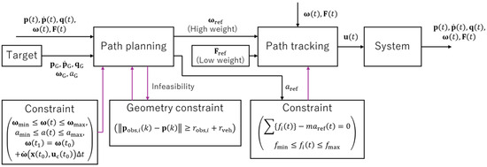
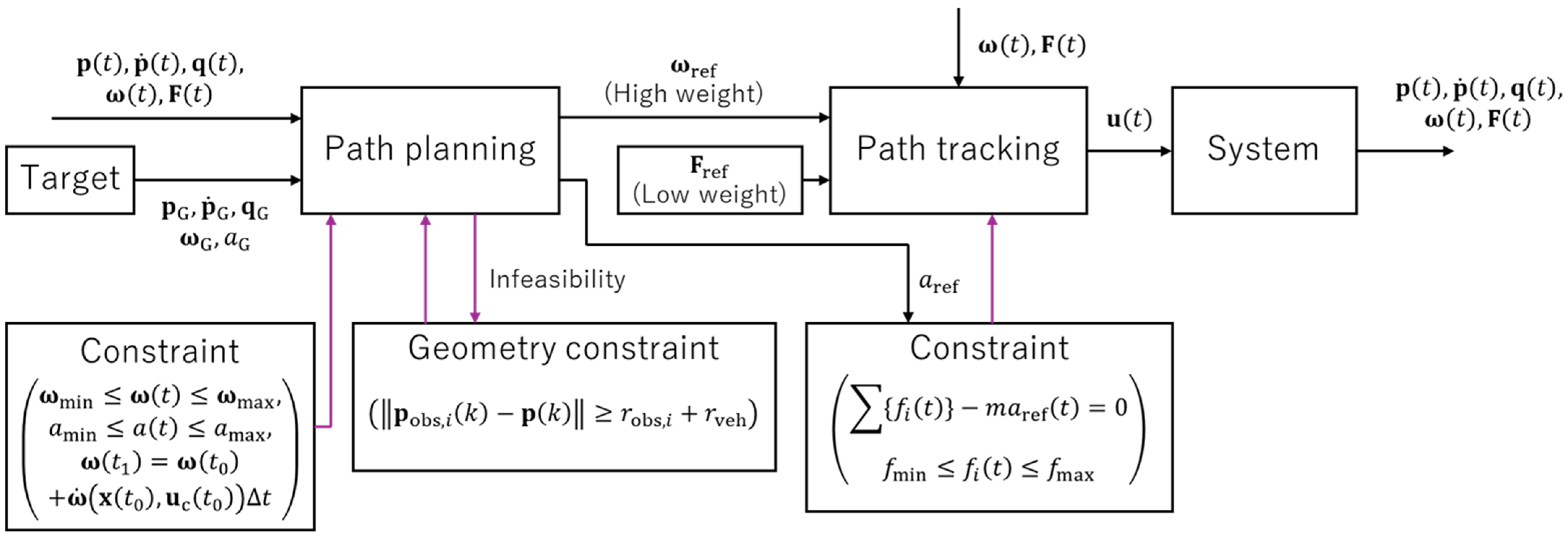
Figure 1 illustrates the overall framework of the path planning and path tracking system. Here, , , , , and denote the target states. In the path tracking stage, appropriate weighting of and is required when applying AL-iLQR.
Figure 1.
Block diagram of path planning and path tracking.
3. Problem Formulation and Solution
This section formulates the constrained trajectory optimization problem and describes the corresponding solution algorithm. The proposed method is categorized as a modified Augmented Lagrangian iterative Linear Quadratic Regulator (AL-iLQR) framework for trajectory optimization under geometric constraints. The constrained optimization problem is handled using the Augmented Lagrangian Method (ALM), while the resulting relaxed subproblems are efficiently solved using iLQR.
3.1. Constrained Optimization Problem for Model Predictive Control
In optimal control theory, a discrete-time nonlinear optimal control problem with constraints is formulated as follows:
where is the index of the discrete time, is the terminal cost, and is the stage cost. The state and control input are denoted by and , respectively. The stacked state and control sequences are defined as, , and . Here, , , , and denote the sets of equality and inequality constraints, respectively. The objective is to determine a control sequence that minimizes .
3.2. Constrained Optimization Algorithm
The constrained optimization problem is transformed into an unconstrained one by constructing the augmented Lagrangian:
where denotes the set of Lagrange multipliers and is the penalty parameter. ALM, summarized in Algorithm 1, seeks a solution that minimizes . The multiplier and penalty parameters are updated according to
where is a constant scaling factor. As , the solution asymptotically satisfies the constraints strictly.
| Algorithm 1: Augmented Lagrangian Method | |
| Inputs: | |
| Outputs: | |
| Procedure: | |
| 1: | |
| 2: | |
| 3: | while |
| 4: | |
| 5: | if the convergence conditions are satisfied |
| 6: | Break |
| 7: | end if |
| 8: | |
| 9: | end while |
3.3. Minimization of the Augmented Lagrangian
To minimize , Differential Dynamic Programming (DDP) [51] and iLQR are employed. In the ALM framework, is minimized while keeping and fixed:
In the trajectory optimization, the value function is defined as
Applying Bellman’s principle of optimality, the following recursion is obtained.
The corresponding active-value function is defined as
Since Equation (28) is nonlinear, a second-order Taylor expansion is employed, as shown in Equation (29).
Equation (28) is a nonlinear problem and must be approximated as follows:
According to iLQR, we assume that the value function can be expressed in quadratic form.
By using Equations (27) and (29),
Note,
When the optimal solution is found, the following equation is satisfied by using Equation (29):
Since may not be a regular matrix, the parameter for regularization is often used,
By using Equations (29), (30) and (40) and ,
The expected decrease in the value function is
Based on the above, iLQR calculates the feedback gains in backward pass, then use those gains to find the input variables that minimize the cost function by using a linear search in forward pass.
where
Algorithm 2 shows the iLQR methods. We define the optimization problem in iLQR in detail.
where are weight matrices, , and the ref means the design values.
| Algorithm 2: iLQR for finding | |
| Inputs: | |
| Outputs: | |
| Procedure: | |
| 1: | |
| 2: | While |
| 3: | in Equation (40) |
| 4: | Equations (36), (37), (48) and (49) |
| 5: | |
| 6: | Calculations from Equations (31)–(35) |
| 7: | ) failed |
| 8: | |
| 9: | |
| 10: | Go to line 5 |
| 11: | end if |
| 12: | Equation (40) |
| 13: | end for |
| 14: | |
| 15: | While |
| 16: | using Equations (15) and (47) |
| 17: | |
| 18: | |
| 19: | |
| 20: | |
| 21: | Break |
| 22: | end if |
| 23: | ) |
| 24: | end while |
| 25: | |
| 26: | Break |
| 27: | end if |
| 28: | |
| 29: | end while |
| 30: | |
4. Our Proposed Method for Feasibility
This section presents the proposed guidance mechanism designed to steer the AL-iLQR algorithm away from infeasible local minima and to improve convergence toward feasible solutions.
Figure 2 illustrates the overall quadrotor system architecture, encompassing the complete pipeline from trajectory planning to trajectory tracking while incorporating the associated constraints. The constraints are visually categorized in the diagram: the left block represents general system constraints; the central block corresponds to position constraints relevant to the path planning stage; and the right block describes constraints imposed during path tracking. When trajectory optimization fails to identify a feasible solution, the proposed method dynamically modifies the geometric constraints. This modification acts as a corrective mechanism by transmitting a guidance signal from the path planning module to the constraint formulation. Note that the left block also includes constraints related to system dynamics.
Figure 2.
Control system of the quadrotor with explicit constraints.
4.1. What Is Feasibility for Collision Avoidance?
General-purpose optimization solvers, such as SQP and IPOPT, often struggle to robustly converge to feasible regions under complex constraints. This difficulty also arises in AL-iLQR, which is employed in this study. The problem is particularly pronounced in collision avoidance problems, which impose the following position constraint.
where denotes the position of the -th obstacle, is the discrete time index, and the collision radii define spherical approximations of the obstacle and the vehicle geometry. While such algorithms can reliably find feasible trajectories in simple scenarios (e.g., a single obstacle), they often converge to infeasible local minima in complex environments with multiple obstacles. This behavior is a direct consequence of their gradient-based nature.
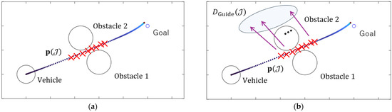
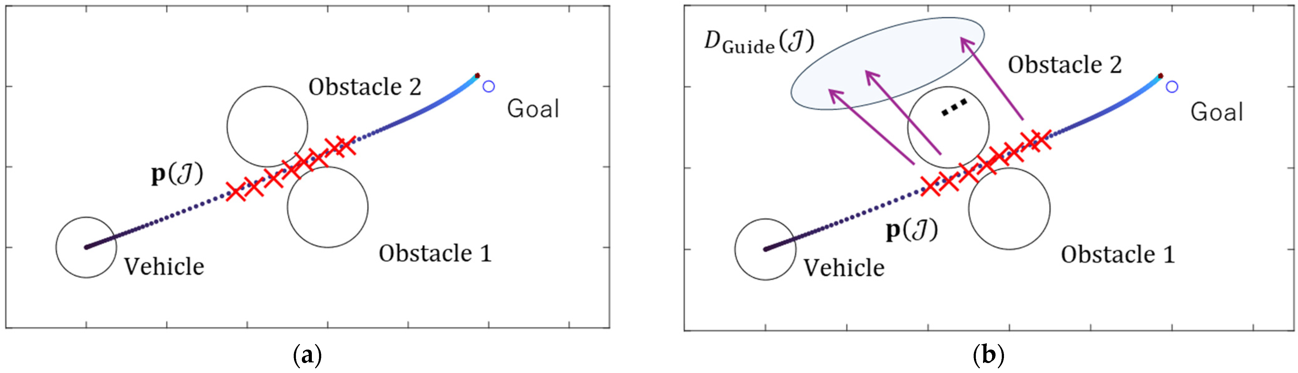
Figure 3a illustrates this failure mode using a two-dimensional example. The color-graded curve extending toward the target represents the predictive trajectory generated by AL-iLQR. The red crosses (×) denote infeasible states that violate the position constraints. This result indicates convergence to an infeasible local minimum.
Figure 3.
Convergence of AL-iLQR to an infeasible local solution in 2D dynamics and the effect of the proposed guidance mechanism. (a) The predicted trajectory (shown with a color gradient), generated during the AL-iLQR iterative process, is blocked by obstacles and converges to an infeasible local minimum (red cross); (b) The proposed guidance mechanism is activated, and a new feasible target region is dynamically generated to steer the trajectory out of the local minimum. The arrows are shown as the directions of the feasible region.
In AL-iLQR, constraint multipliers are initialized with small values and gradually increased. Consequently, the algorithm initially solves a relaxed problem in which constraint violations have only a weak influence on the cost function. As a result, even when starting from a feasible initial guess, early iterations tend to prioritize minimizing the primary cost over satisfying constraints. Once the trajectory converges to an infeasible region, such as that shown in Figure 3a, subsequent increases in the multipliers are often insufficient to escape the infeasible solution.
Therefore, the solution we propose is to actively guide the predictive trajectory into the feasible region during the iterative optimization process. Our guidance mechanism is represented by the region in Figure 3b. constitutes the set of discrete time indices of constraint violations that are highly unlikely to be resolved by further AL-iLQR iterations.
To address this problem, we propose actively guiding the predictive trajectory into a feasible region during the iterative optimization process. This guidance mechanism is illustrated by the region in Figure 3b. The set consists of discrete time indices at which constraint violations are unlikely to be resolved by further AL-iLQR iterations alone.
To identify such indices, we first define the set of active constraints at each time step.
where
Here, denotes the number of obstacles. If , the trajectory is feasible at time ; if , feasibility can often be recovered through iterative optimization. On the other hand, when only one geometric constraint is active, AL-iLQR can successfully find a solution by continuously deforming the trajectory using gradient information, assuming spherical obstacles. In contrast, when two or more constraints are active, the spatial arrangement of the obstacles can cause the gradient vectors to cancel each other out in the augmented Lagrangian method. Consequently, there is no guarantee that the gradient direction calculated by AL-iLQR will coincide with the correct direction toward the feasible region. Accordingly, the index set is defined as
4.2. How to Find
The challenge of determining extends beyond identifying any feasible solution; it lies in simultaneously satisfying constraints while optimizing the mission cost. The objective is not to compute a single optimal trajectory, but rather to estimate a region in which optimal solutions are likely to be distributed. To this end, we employ a sampling-based solver, Model Predictive Path Integral control (MPPI), which is well suited for rapidly approximating the distribution of optimal solutions.
The MPPI cost function is defined as
Here, is a constant penalty parameter. MPPI enforces input constraints by clamping sampled inputs that fall outside the admissible range. Assuming the sampled input follows a multivariate Gaussian distribution centered at the mean input with covariance , the sampling distribution is given by
The optimal control sequence is obtained by solving
where is the distribution that is described by . According to the variational inference theory, minimizing KL-divergence yields the optimal solution. Under the Law of Large Numbers, the sample-based approximation used in MPPI converges to the true expected value as the number of samples increases. Note, the law does not guarantee convergence to the global optimum. Algorithm 3 shows the MPPI algorithm [49].
The optimal state sequence is then obtained from , and the guidance region is determined such that it contains .
| Algorithm 3: Model Predictive Path Integration (MPPI) | |
| Inputs: | |
| Outputs: | |
| Procedure: | |
| 1: | // Sampling number |
| 2: | |
| 3: | |
| 4: | |
| 5: | |
| 6: | |
| 7: | |
| 8: | |
| 9: | |
| 10: | end for |
| 11: | |
| 12: | end for |
| 13: | |
| 14: | |
| 15: | |
| 16: | |
| 17: | |
| 18: | |
| 19: | end for |
| 20: | |
4.3. Integration of into AL-iLQR
Based on the sampled inputs generated by MPPI, we obtain an estimate of the optimal distribution . The guidance region is then integrated into the AL-iLQR framework. The key observation is that AL-iLQR converges efficiently to an optimal solution as long as the trajectory remains within the feasible region. Therefore, it is sufficient to guide the trajectory toward feasibility rather than explicitly solving the global constrained problem. The guidance region is defined as
where
Here, corresponds to the MPPI-derived reference position . The guidance radius , selected to be smaller than the obstacle geometry, is set equal to the collision radius of the controlled vehicle.
Since may vary significantly between AL-iLQR iterations—especially in multimodal solution spaces—reusing multipliers from previous iterations can hinder convergence. Therefore, we redefine the augmented Lagrangian as
The penalty parameter is updated according to
where is chosen such that . Satisfying the guidance constraint in Equation (62) becomes equivalent to satisfying the original collision constraint in Equation (52) in later iterations, once the AL-iLQR multipliers have sufficiently increased. If , the guidance constraint is omitted.
When GCO is activated, the guidance constraint is penalized more aggressively than the original constraints, thereby prioritizing feasibility restoration. If the solution later drifts back into infeasible regions, the guidance mechanism is reactivated. Once convergence within the feasible domain is imminent, the guidance constraint is permanently deactivated.
Unlike standard augmented Lagrangian (AL) constraints, the proposed guidance constraint is incorporated directly into the cost function as a penalty term rather than through Lagrange multipliers. From a numerical standpoint, it is treated as an inequality constraint whose associated multiplier is intentionally fixed to zero.
In the proposed scheme, the guidance mechanism is integrated into the AL-iLQR optimizer. While the original collision avoidance constraints in Equation (52) are handled using the full AL formulation with Lagrange multipliers , the guidance constraint in Equation (62) is excluded from the AL framework and instead added directly to the AL-iLQR cost function as a simple penalty term. The guidance constraint is introduced as a temporary penalty term to assist the optimization process when the solver encounters a solution that may yield an infeasible local minima during the AL-iLQR iterations. Importantly, the guidance constraint is designed to remain inactive in the vicinity of feasible solutions. Since the optimal trajectory must satisfy the original geometric constraints, the guidance constraint naturally becomes inactive near the final solution. Therefore, the final solution satisfies the Karush–Kuhn–Tucker (KKT) conditions associated with the original optimization problem. In addition, the margin parameter ensures that the feasible region around the optimal trajectory remains inside the region where the guidance constraint is inactive.
The proposed framework involves several parameters, such as the guidance margin , the sampling distribution parameters in MPPI, and the penalty weights used in the augmented Lagrangian formulation. The guidance margin mainly determines the activation region of the guidance mechanism, while the AL-iLQR refinement step ensures that the final trajectory satisfies the original geometric constraints. As a result, the final solution is not highly sensitive to the exact value of this parameter. Similarly, the MPPI sampling parameters primarily influence the exploration behavior during the guidance phase, but once a feasible trajectory is identified, the optimization process proceeds using the standard AL-iLQR framework. The overall guidance algorithm is summarized in Algorithms 4 and 5.
| Algorithm 4: Modified AL-iLQR (Our proposed method) | |
| Inputs: | |
| Outputs: | |
| Procedure: | |
| 1: | |
| 2: | |
| 3: | |
| 4: | |
| 5: | while |
| 6: | using iLQR |
| 7: | if the convergence conditions are satisfied |
| 8: | Break |
| 9: | end if |
| 10: | |
| 11: | using Equations (21), (22) and (66) |
| 12: | corresponds to Equation (62) |
| 13: | end while |
| 14: | |
| Algorithm 5: Constraint Parameters Update for Feasibility (CPUF) | |
| Inputs: | |
| Outputs: | |
| Procedure: | |
| 1: | |
| 2: | |
| 3: | |
| 4: | |
| 5: | |
| 6: | |
| 7: | |
| 8: | |
| 9: | |
| 10: | end if |
| 11: | end for |
| 12: | |
| 13: | end if |
| 14: | |
5. Simulation Results and Discussion
The effectiveness of the proposed method is verified through numerical simulations. As a preliminary validation, the proposed approach is first applied to a two-dimensional (2D) dynamical system. This simplified setting allows the trajectory optimization behavior to be evaluated on a planar domain while decoupling the complex three-dimensional dynamics associated with UAVs. In particular, the 2D simulation facilitates visualization of the optimization process and clarifies how the solution is deformed during iterative updates when the guidance constraint optimization (GCO) is activated (see Appendix A).
Subsequently, quadrotor simulations are conducted to confirm that the generated trajectories are feasible for path tracking control and result in successful collision avoidance. The quadrotor trajectory optimization problem is formulated as
where and are positive semidefinite weight matrices. To reduce computational cost, the terminal constraints do not include GCO.
In the ALM implementation, a maximum iteration limit is employed instead of checking the KKT conditions in order to simplify the optimization procedure. All simulations were conducted on a laptop equipped with an Intel Core i7-12650H (2.30 GHz) processor, 16 GB RAM, using MATLAB R2024b.
5.1. 2D Trajectory Optimization
This 2D trajectory optimization problem is introduced to provide an intuitive and computationally lightweight validation of the proposed guidance mechanism. By restricting the system dynamics to a planar model, we decouple the core trajectory optimization behavior from the additional complexities introduced by full 3D quadrotor dynamics, such as attitude coupling and thrust vectoring. The purpose of this simplified model is not to replicate realistic UAV dynamics, but to clearly visualize how the proposed guidance constraint (GCO) influences the deformation of trajectories during the iterative optimization process. In particular, the 2D setting allows us to isolate and analyze failure modes related to non-convex geometric constraints and local infeasible minima, which are also present in higher-dimensional systems. Importantly, the same optimization framework, constraint formulation, and guidance logic are retained when extending to the full quadrotor model in Section 5.2. Therefore, the 2D simulation serves as a conceptual validation of the proposed method, while the quadrotor simulation demonstrates its practical applicability under realistic dynamics.
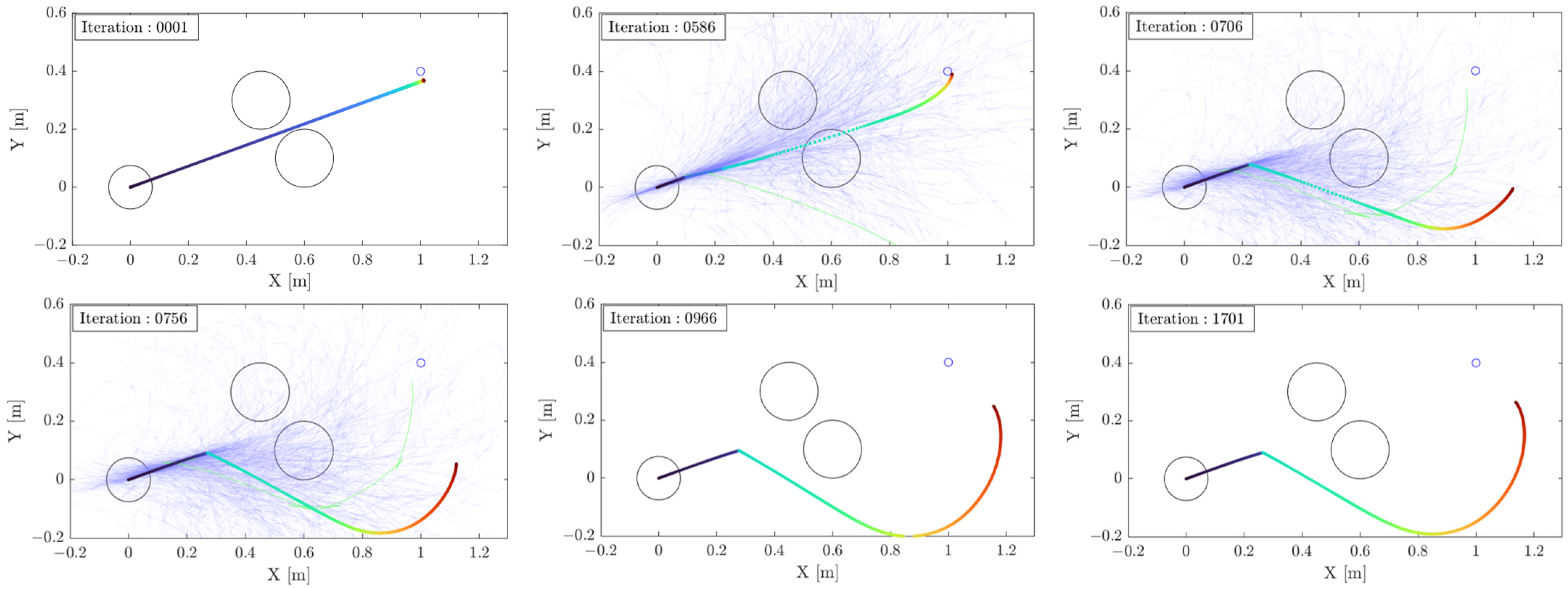
The simulation parameters are summarized in Table A1, Table A2 and Table A3, and the positional configuration is identical to that shown in Figure 3. The results obtained using the proposed method under box input constraints and inequality constraints in Equation (52) are presented in Figure 4, Figure 5, Figure A1a and Figure A2a and Table A4(a). Although standard MPPI is often regarded as ill-suited for multimodal problems due to its unimodal Gaussian sampling assumption, the numerical results demonstrate that a feasible trajectory can still be obtained while preserving near-optimality. Notably, the SQP solver implemented in MATLAB’s fmincon failed to solve the same problem within several hours.
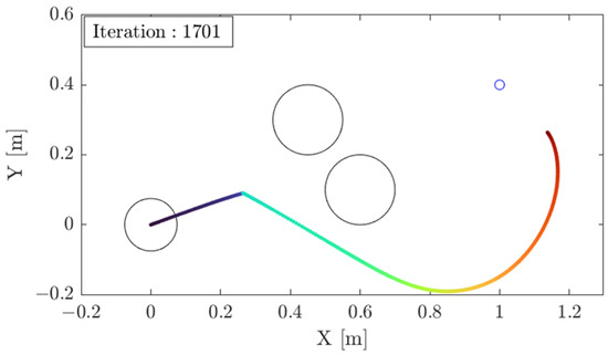
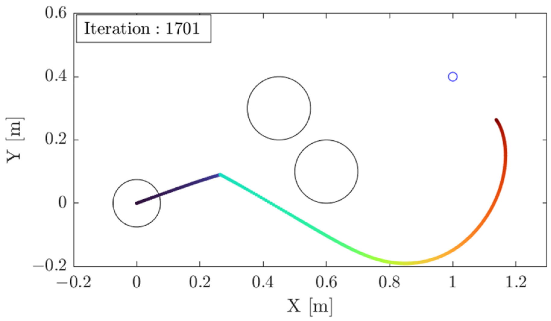
Figure 4.
The optimal predicted trajectory generated by the proposed method (visualized with a color gradient; where cool colors indicate the near future and warm colors represent the distant future). Here, Iteration denotes the number of cost convergence checks () within the AL-iLQR process.
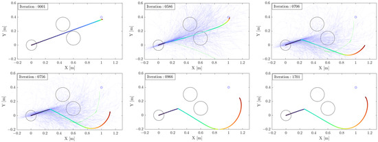
Figure 5.
Trajectory updates during the iterative optimization process of AL-iLQR. The AL-iLQR solution is visualized with a color gradient, where cool-colored dots indicate the near future and warm-colored dots represent the distant future. The thin blue and green lines denote MPPI sample trajectories and the MPPI optimal trajectory, respectively. The rest of the explanation is the same as in Figure 3.
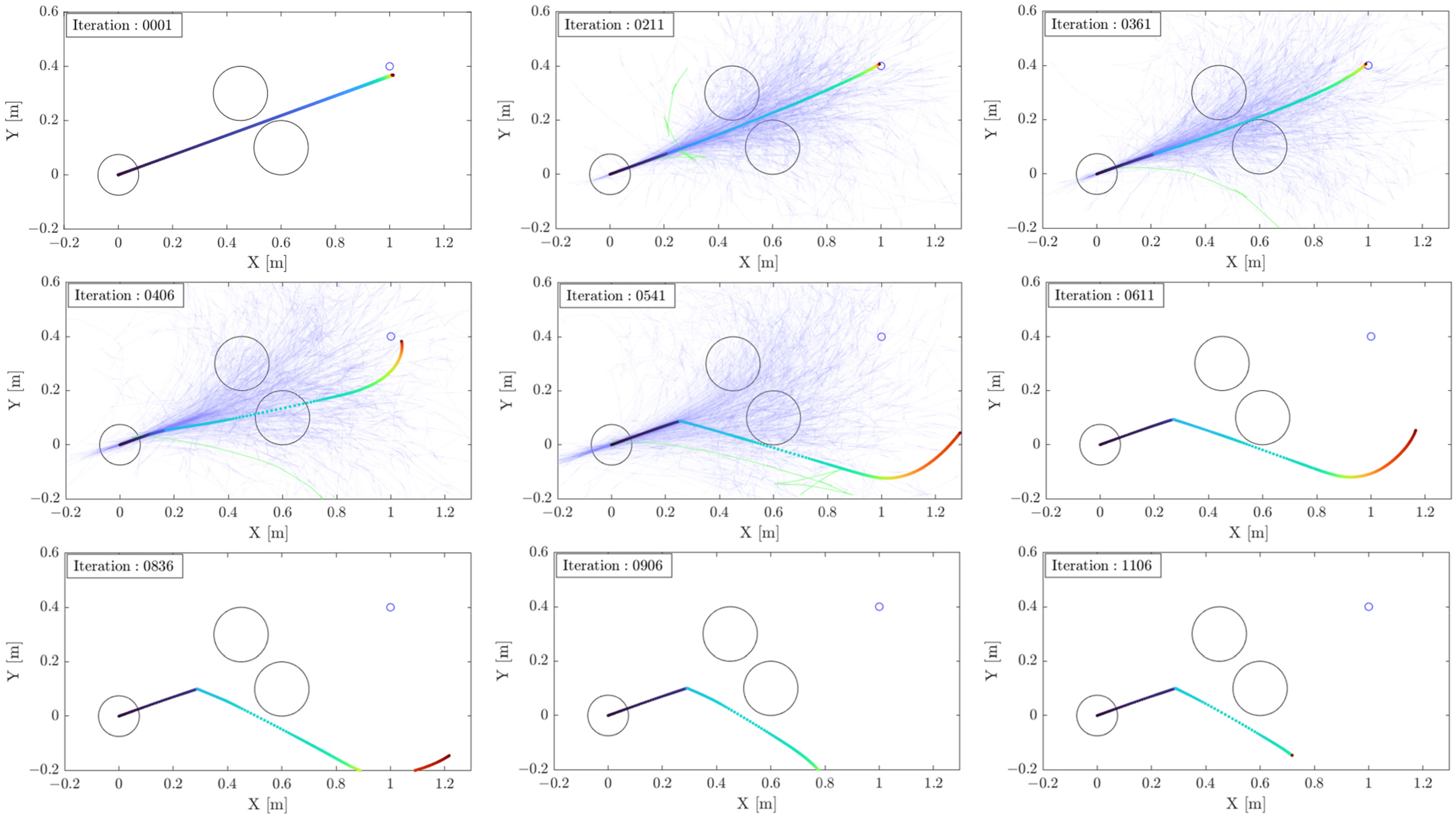
Figure 4 shows the optimal predicted trajectory as a gradient-colored curve. The resulting trajectory appears non-smooth and seems to converge to a local minimum. Indeed, due to the stochastic nature of MPPI sampling, multiple distinct local solutions were obtained across different trials, as illustrated in Figure A1b, Figure A2b and Figure A3, and Table A4(b). It was shown that the proposed method does not necessarily yield a globally optimal solution. In the MPPI sampling process, soft input constraints () are employed to enable broader exploration of the positional space, without affecting the satisfaction of input constraints in the final optimized solution.
Figure 5 illustrates the evolution of the trajectory throughout the iterative optimization process. In the initial iteration, the standard AL-iLQR yields an infeasible solution. Upon updating the ALM multipliers and penalties, the solver detects the violation set , which triggers the generation of GCO. In the early stages, the solution remains trapped in the infeasible region because the priority difference between GCO and the original constraints is insufficient. As iterations proceed, GCO is assigned higher priority, allowing the solver to escape the infeasible region and converge to a feasible trajectory. Once the multipliers and penalties associated with the positional constraints become sufficiently large, GCO is deactivated to avoid interfering with the primary cost optimization. If the solution subsequently regresses into an infeasible region, GCO is reactivated to restore feasibility.
5.2. Quadrotor Simulation
5.2.1. Simulation Configuration
Numerical simulations are conducted in an environment designed to induce infeasible trajectories, using a framework intended for practical deployment on real hardware, shown in Figure 1. The quadrotor task configuration is summarized in Table 1, and the quadrotor parameters are adopted from [52], as listed in Table 2.
Table 1.
Problem setup of the quadrotor trajectory optimization.
Table 2.
Model parameters of the quadrotor.
To reduce computational complexity, the cost function is evaluated by directly subtracting quaternion values, neglecting quaternion error dynamics. In addition, the following constraint is imposed during path planning to ensure consistency between the path planning and path tracking models:
where denotes the control period, and and represent consecutive time steps. For optimization, the collision detection radius is set to , while a reduced boundary of is used in numerical simulations to incorporate a safety margin (Table 3). The MPPI and AL-iLQR parameters used for path planning are listed in Table 4. The penalty associated with GCO is increased more aggressively than the other penalties, satisfying .
Table 3.
Environments used in the numerical simulations.
Table 4.
MPPI and AL-iLQR configurations for path planning.
The tracking algorithm parameters are summarized in Table 5. Standard AL-iLQR was employed to calculate the optimal control inputs for the quadrotor. Importantly, the computational cost of path tracking is negligible relative to that of path planning (Appendix B).
Table 5.
Parameter settings for AL-iLQR-based path tracking.
5.2.2. Numerical Simulation
While Section 5.1 examined optimization results at a single time instance, this section considers a continuous transport mission in which the proposed method solves the trajectory optimization problem at every simulation time step. The Lagrange multipliers are re-initialized at each step because changes in the environment and optimal trajectory render multipliers from the previous step ineffective. Although reusing multipliers could reduce computational cost, re-initialization is adopted to improve robustness. In particular, this setup allows us to test whether the method can still generate feasible trajectories when the initial guess is infeasible, which may occur in the presence of modeling errors or dynamic obstacles. Once a feasible trajectory is obtained, the multipliers from the previous step typically provide an accurate initial guess, and the guidance mechanism is rarely activated. In such situations, the solver can operate with the computational efficiency of the standard AL-iLQR framework.
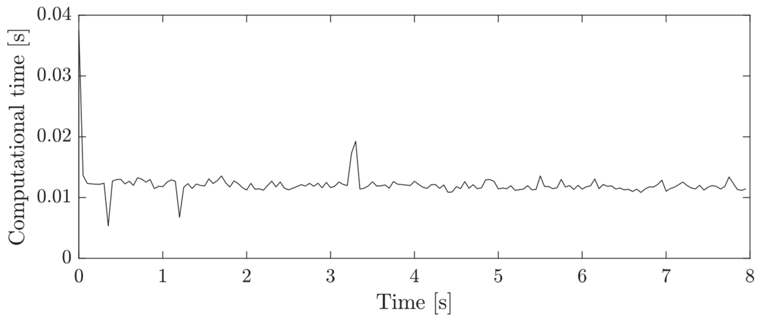
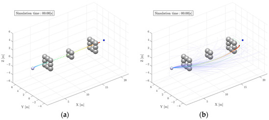
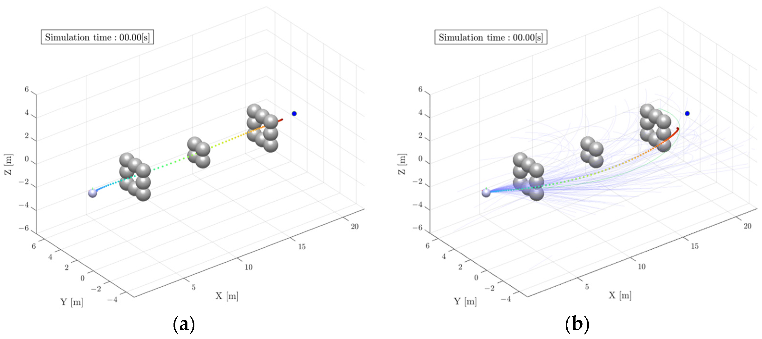
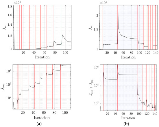
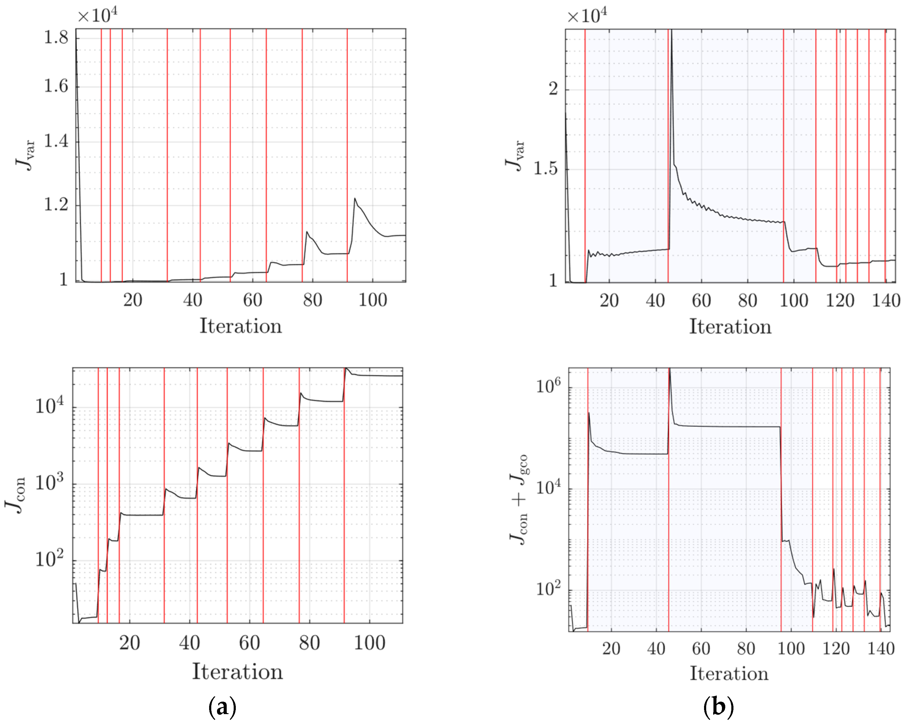
Figure 6 shows the optimal predicted trajectories for path planning at the initial time step. Figure 6a depicts an infeasible trajectory generated by standard AL-iLQR, whereas Figure 6b shows that the proposed method successfully finds a feasible solution. The proposed method successfully found a feasible solution. Figure 7 illustrates the cost evolution during the iterative process corresponding to the result in Figure 6. The red lines indicate the timing of multiplier and penalty updates, and the intervals between these lines correspond to the iLQR iterations. In Figure 7a, the costs increase during the multiplier and penalty updates due to convergence to a local minimum. In Figure 7b, the thin blue regions between the red lines indicate periods of GCO activation. When a potential infeasible solution is detected, GCO is activated to initiate the guidance process. The trajectory effectively bypasses obstacles and is guided toward a feasible region as the multiplier and penalty values increase. Subsequently, GCO is deactivated, and constraint satisfaction improves iteratively. The narrow intervals between the red lines suggest that a local minimum is identified rapidly.
Figure 6.
Snapshots of trajectory predictions (shown as a gradient-colored dotted line; where cool colors indicate the near future and warm colors represent the distant future) in path planning. (a) AL-iLQR without GCO; (b) The proposed method with GCO. The blue and gray objects represent the quadrotor and the obstacles, respectively. The blue dot marks the target point. The green line denotes the optimal solution, while the thin blue lines represent the MPPI samples.
Figure 7.
Cost evolution during the iterative process. (a) AL-iLQR without GCO; (b) Proposed method with GCO. The thin blue region denotes the detection of set and GCO activation, while red lines mark the timing of multipliers and penalty updates. Note: Line search steps in AL-iLQR are not included in the iteration count.
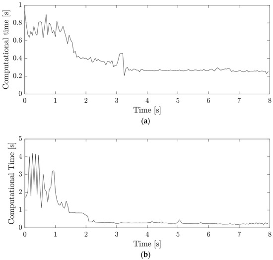
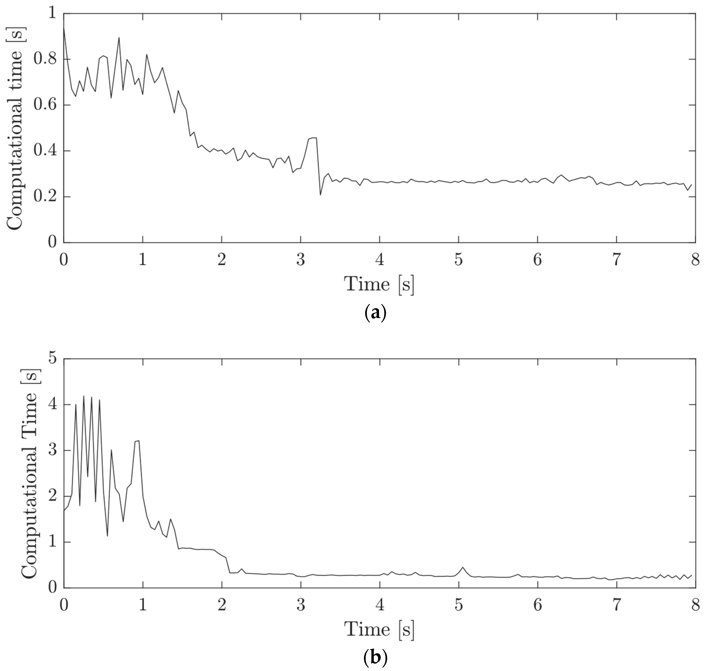
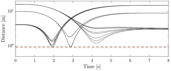
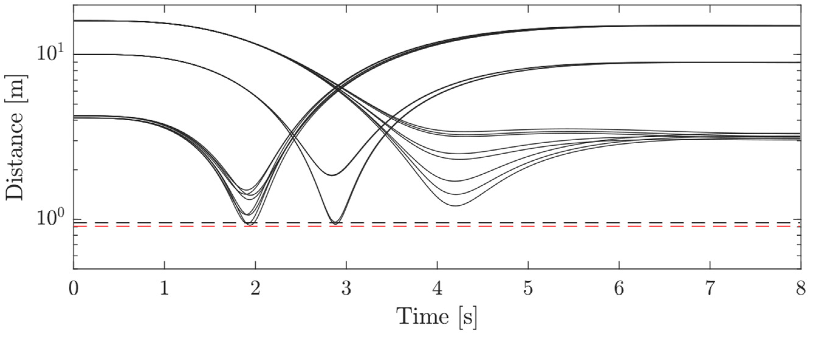
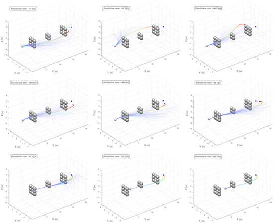
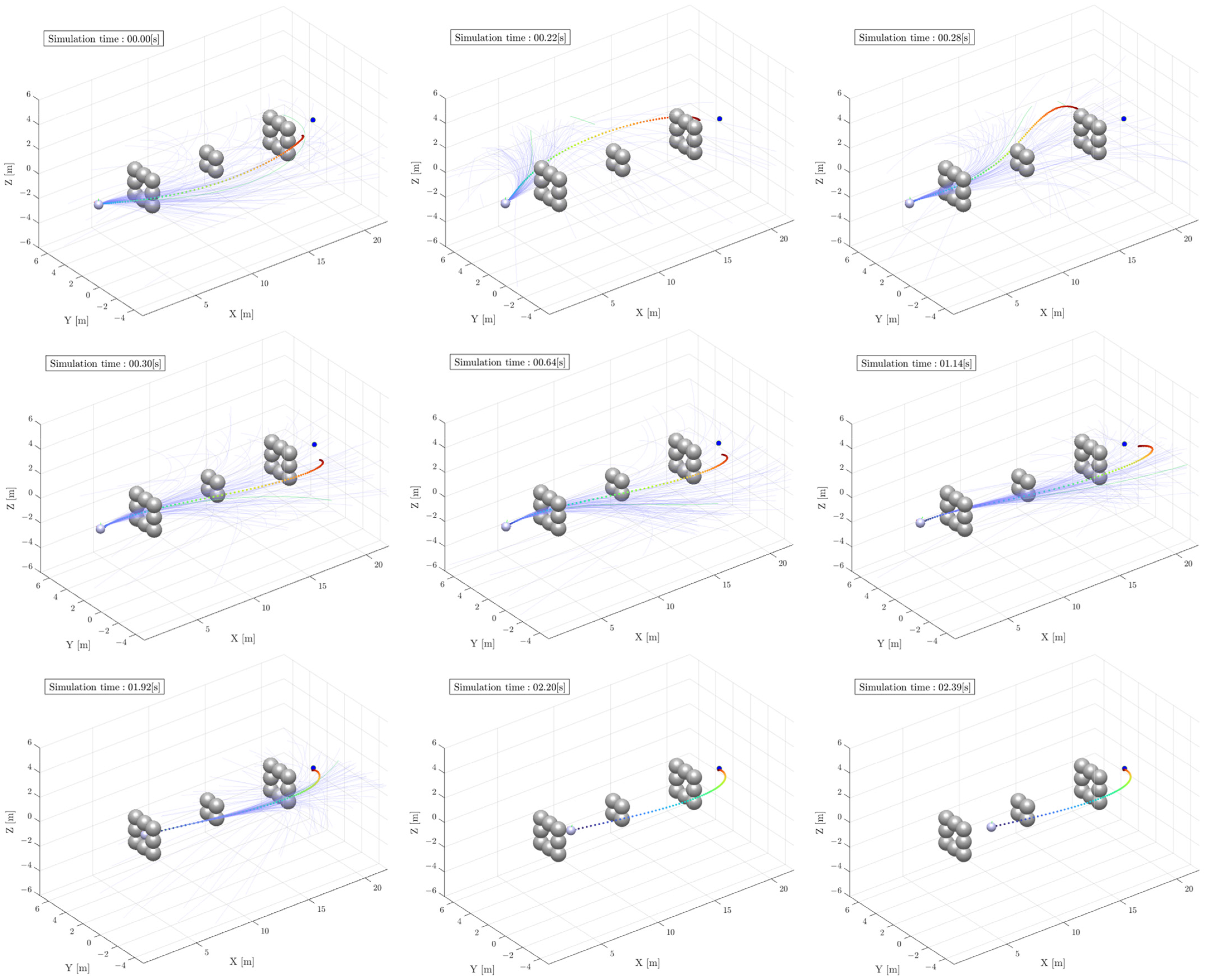
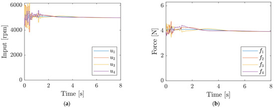
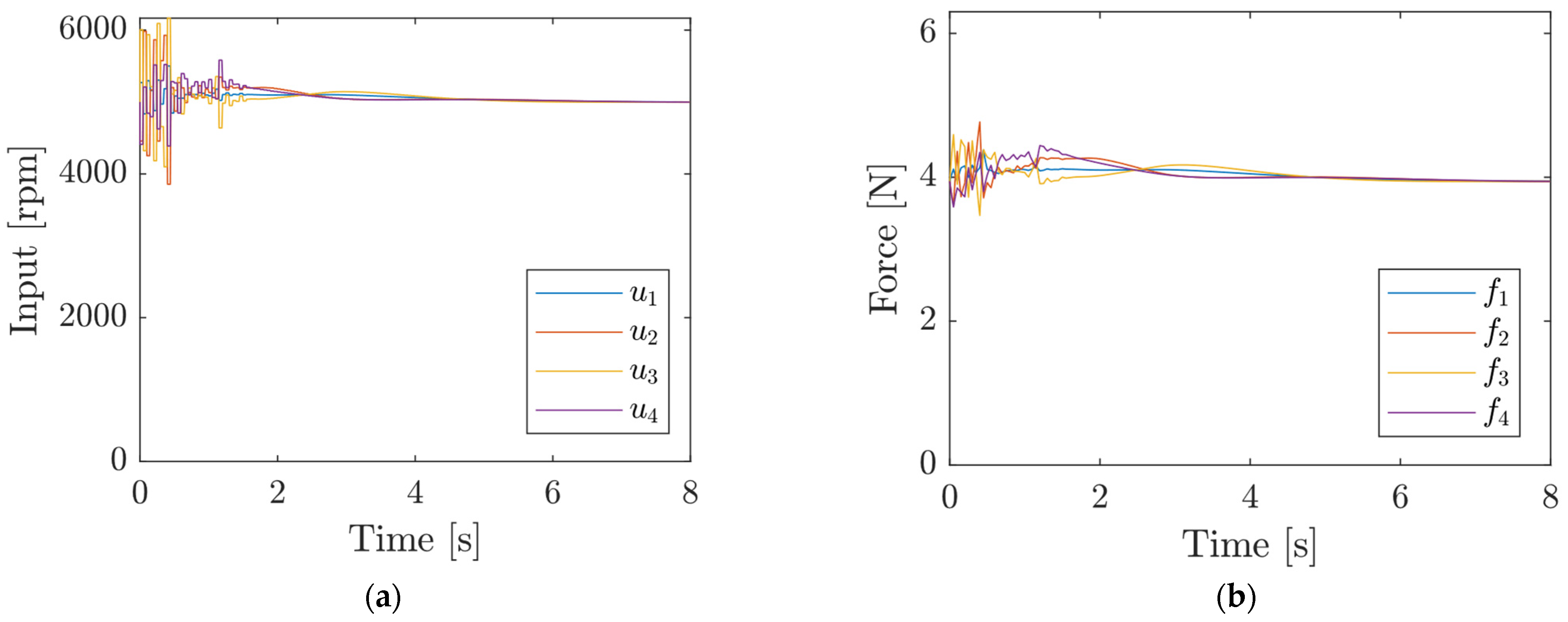
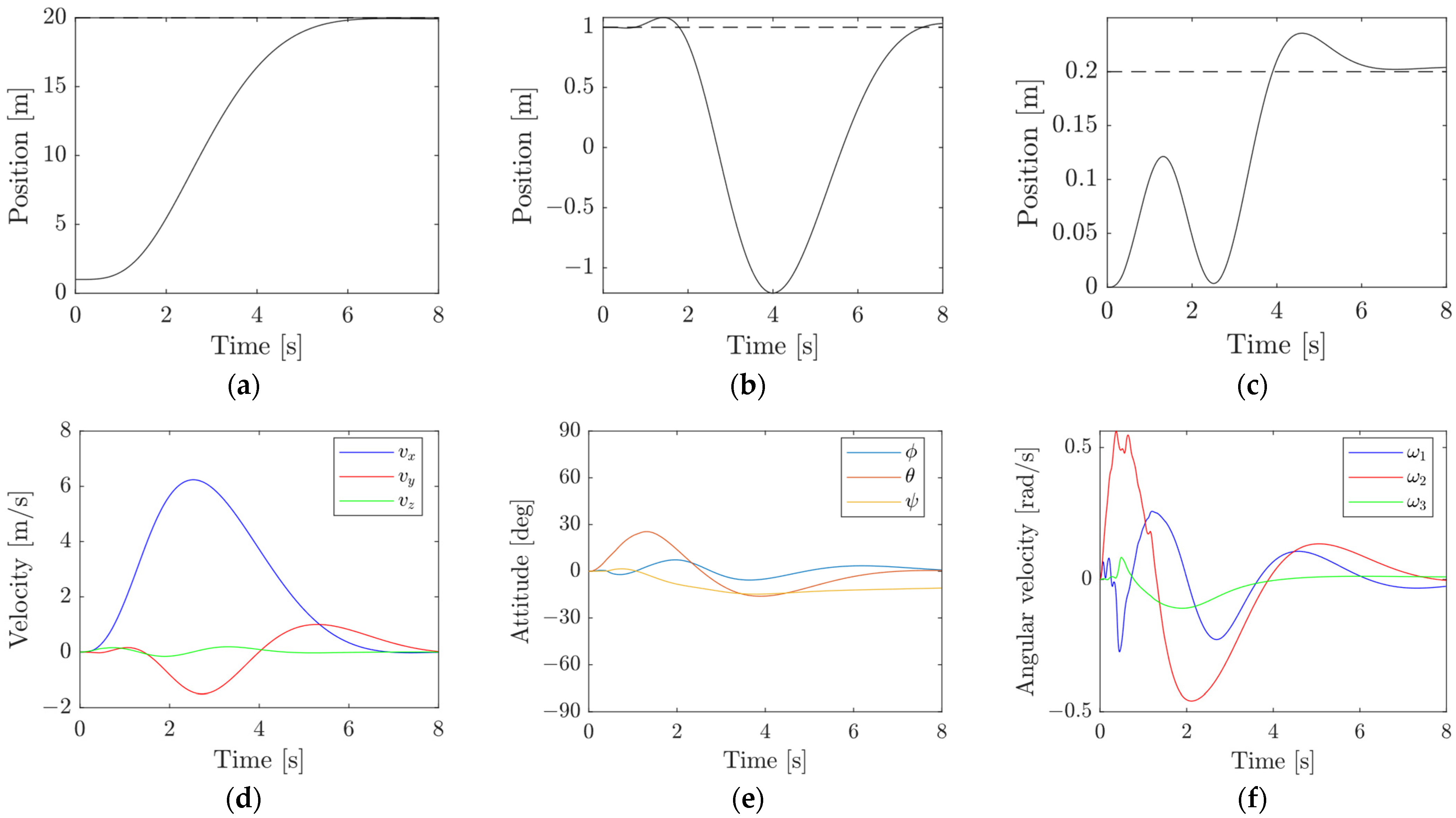
Figure 8, Figure 9, Figure 10, Figure 11 and Figure 12 present the quadrotor control results obtained using the proposed method. Figure 8 compares the computational time per simulation step for (a) standard AL-iLQR and (b) the proposed method. The computational cost decreases as the number of active constraints is reduced. Figure 9 shows the minimum distance between the quadrotor and obstacles, where the red dotted line denotes the collision detection boundary. The results confirm collision-free operation. The black dotted line represents the boundary used during path planning optimization. Figure 10 shows snapshots of the optimized trajectories, demonstrating successful obstacle avoidance despite modeling simplifications in the path planning stage. These simplifications introduce transient fluctuations in the optimal solution, particularly during periods of rapid input variation; however, no infeasible trajectories are observed. The absence of MPPI trajectories in the snapshots indicates that GCO is inactive at those time steps. Figure 11 illustrates the control commands and resulting thruster states, while Figure 12 presents the time histories of state variables, including position and target position.
Figure 8.
Computational time of the path planning and path tracking at each time step. (a) AL-iLQR without GCO; (b) The proposed method with GCO.
Figure 9.
Distance between the quadrotor and the obstacle. Black and red dashed lines indicate the AL-iLQR constraint boundary , and the collision detection boundary respectively.
Figure 10.
Snapshots of the numerical simulation. The disappearance of MPPI trajectories at certain time steps indicates that the AL-iLQR solver successfully found a solution without GCO. The AL-iLQR solution is visualized with a color gradient, where cool-colored dots indicate the near future and warm-colored dots represent the distant future. The thin blue and green lines denote MPPI sample trajectories and the MPPI optimal trajectory, respectively.
Figure 11.
Time histories of command inputs and thrusts for the quadrotor system. (a) Command inputs; (b) Resulting thrusts generated by the inputs.
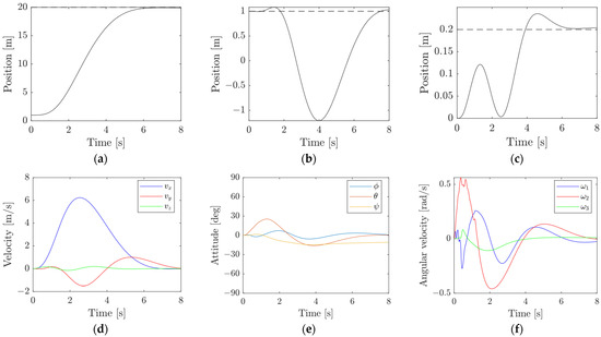
Figure 12.
Time histories of state variables. (a–c) represent the quadrotor position along the X, Y, and Z axis, respectively. (d–f) additional state variables, where (e) represents Euler angles. Dotted lines denote the target states.
The numerical simulations demonstrate that the proposed method can reliably detect potentially infeasible solutions and actively guide trajectories toward feasible regions during optimization. Collision avoidance problems are effectively resolved through the proposed framework, and the method naturally accommodates dynamic obstacles owing to its simple and flexible constraint formulation.
6. Conclusions
This paper proposed a practical trajectory optimization framework for improving feasibility in constrained nonlinear optimal control problems for agile UAVs. The key challenge addressed in this study is the tendency of gradient-based trajectory optimization methods, such as AL-iLQR, to converge to infeasible local minima in the presence of highly non-convex geometric constraints arising from obstacle avoidance. To mitigate this problem, we introduced a plugin-style guidance mechanism that integrates Model Predictive Path Integral (MPPI) control into the AL-iLQR iteration process. MPPI is employed as a fast sampling-based method to explore feasible regions of the trajectory space, while AL-iLQR is used to efficiently refine locally optimal solutions with high numerical accuracy. By decoupling feasibility exploration from local optimal refinement, the proposed method enhances the robustness of trajectory optimization without requiring fundamental modifications to the underlying solver structure. The effectiveness of the proposed approach was demonstrated through numerical simulations involving both simplified two-dimensional dynamics and full quadrotor models. The results showed that the proposed method converges to feasible and dynamically consistent trajectories significantly more reliably than standard AL-iLQR, even in scenarios with multiple obstacles and complex constraint interactions. Furthermore, the proposed guidance mechanism can be activated and deactivated adaptively during the optimization process, enabling efficient real-time computation while preserving solution quality.
It should be emphasized that the proposed method does not aim to provide theoretical guarantees of global optimality. Instead, it is designed as a practical and computationally efficient strategy for improving feasibility and robustness in real-time UAV trajectory optimization. Future work includes theoretical analysis of the guidance mechanism, extension to more complex dynamic environments, and experimental validation on real UAV platforms.
Author Contributions
Conceptualization, S.K. and K.M.; Methodology, S.K.; Software, S.K.; Writing—original draft, S.K.; Writing—review & editing, K.U.; Supervision, K.U.; Project administration, K.U. All authors have read and agreed to the published version of the manuscript.
Funding
This research received no external funding.
Data Availability Statement
The original contributions presented in this study are included in the article. Further inquiries can be directed to the corresponding author.
Conflicts of Interest
The authors declare no conflict of interest.
Appendix A. 2D System Model
The system dynamics considered in Appendix A are two-dimensional. The state value is defined as , where is the position, the velocity, the attitude angle, the angular velocity. The control inputs are modeled as virtual wheel accelerations, neglecting detailed motor and drive-train dynamics for simplicity. Specifically, , where and represent the longitudinal accelerations generated by the left and right wheels, respectively. These inputs are treated as directly controllable variables in the trajectory optimization. The system dynamics are given by
where is a coefficient of dynamics, and .
Table A1.
Problem setup for the numerical simulation.
Table A2.
Parameters of the controlled system.
Table A3.
MPPI and AL-iLQR configurations for 2D simulation.
Table A4.
Numerical optimization results.
Figure A1.
Distinct local solutions arising from the stochastic nature of MPPI sampling in an identical environment. (a) Trial 1; (b) Trial 2. The AL-iLQR solution is visualized with a color gradient, where cool-colored dots indicate the near future and warm-colored dots represent the distant future. The rest of the explanation is the same as in Figure 3.
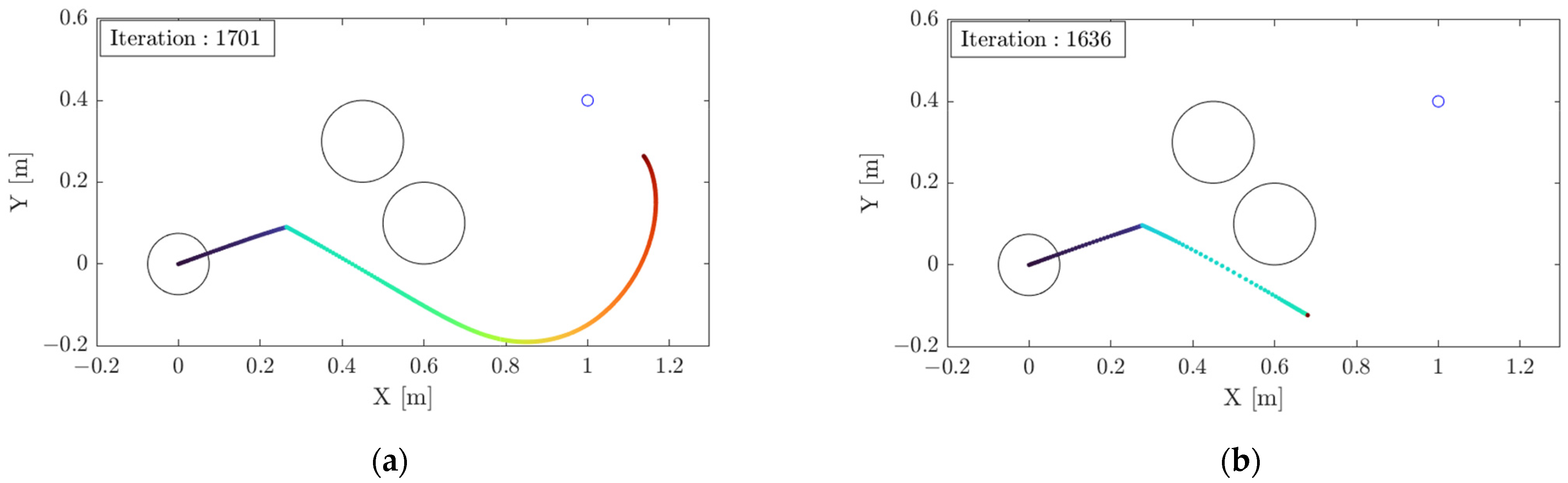
Figure A2.
Predicted states and inputs. (a) Trial 1; (b) Trial 2.
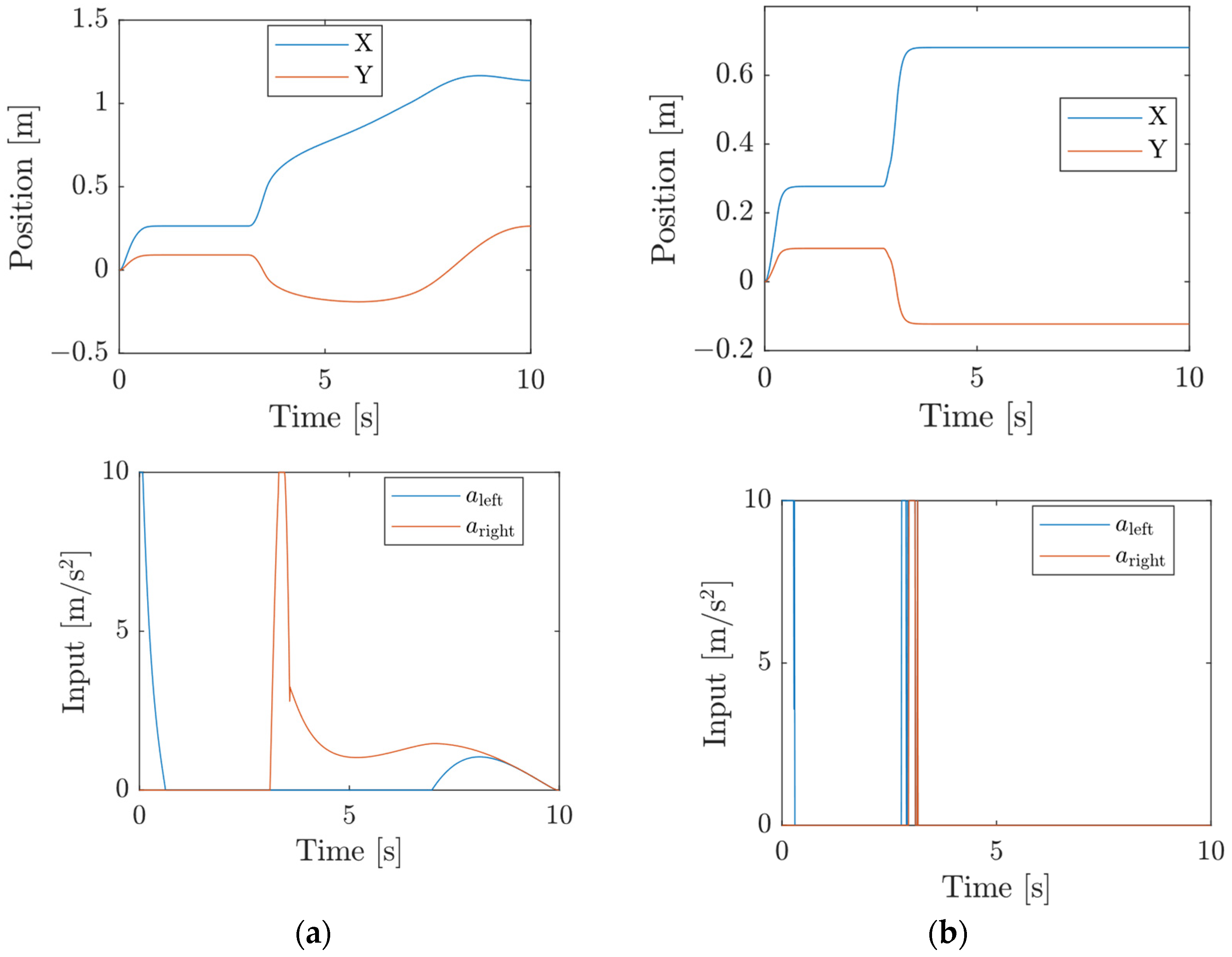
Figure A3.
The optimization process of Trial 2. The AL-iLQR solution is visualized with a color gradient, where cool-colored dots indicate the near future and warm-colored dots represent the distant future. The rest of the explanation is the same as in Figure 3.
Appendix B. Quadrotor Path Tracking Results
Appendix B shows the numerical results of path tracking. Figure A4 shows the magnitude of constraint violations of the path tracking at each simulation time, and Figure A5 illustrates the computation time required for path tracking. Because the upper and lower bounds of the thrust constraints are strictly satisfied at all times, the observed violations stem entirely from the equality constraint presented in Equation (12).
Figure A4.
Maximum constraint violation of the path tracking at each time step in our proposed method.
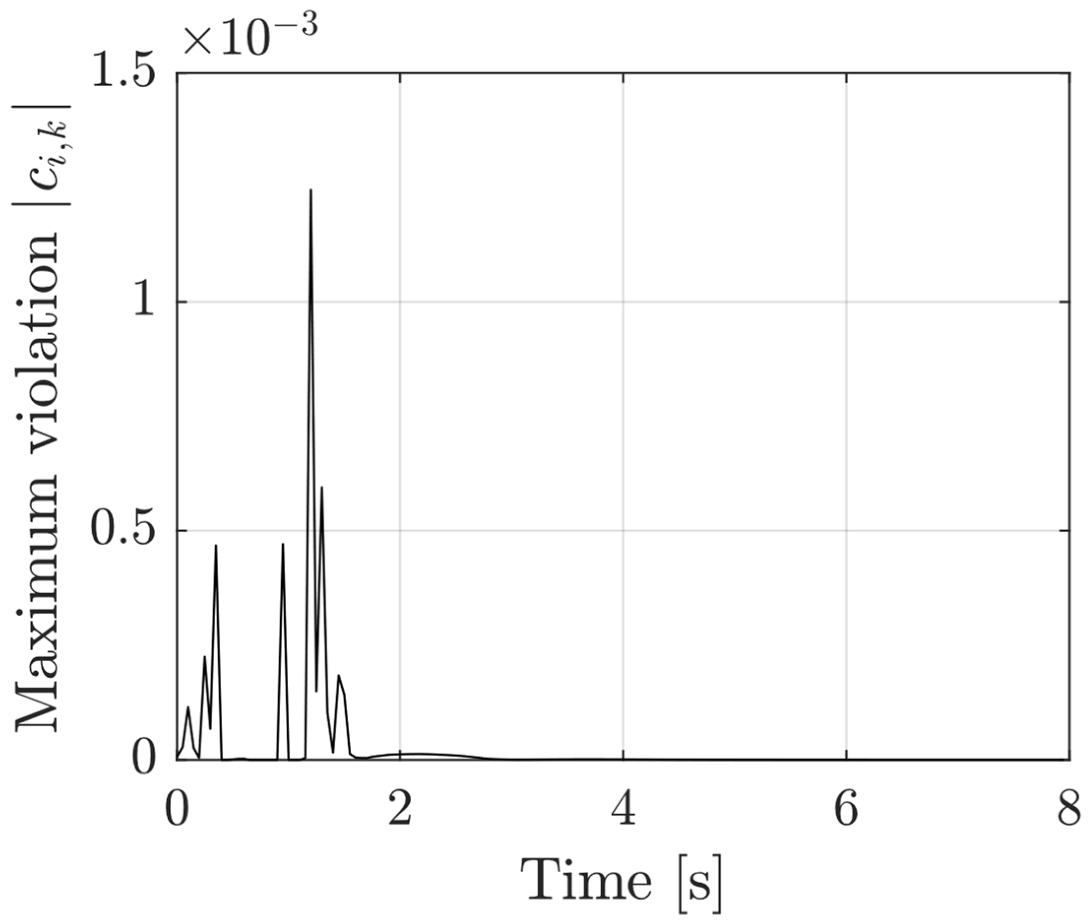
Figure A5.
Computational time of the path tracking at each time step in our proposed method.
References
- Zhao, Z.; Zhang, X.; Fang, H.; Yang, Q. Distributed Formation Planning for Unmanned Aerial Vehicles. Drones 2025, 9, 306. [Google Scholar] [CrossRef] [Scilit]
- Tripicchio, P.; Unetti, M.; D’Avella, S.; Avizzano, C.A. Smooth Coverage Path Planning for UAVs with Model Predictive Control Trajectory Tracking. Electronics 2023, 12, 2310. [Google Scholar] [CrossRef] [Scilit]
- Rubinacci, R.; Nazzari, A.; Lovera, M. Anytime Trajectory Optimization for Multi-Drone Systems With Guaranteed Collision Avoidance. IEEE Control Syst. Lett. 2025, 9, 1255–1260. [Google Scholar] [CrossRef] [Scilit]
- Peng, H.; Huo, M.; He, Y.; Liu, Z. Multiple UAVs collision avoidance trajectory coordination using distributed receding horizon optimization. In Proceedings of the 10th World Congress on Intelligent Control and Automation, Beijing, China, 6–8 July 2012; pp. 3999–4003. [Google Scholar] [CrossRef] [Scilit]
- Dai, S.; Zhao, C.; Ding, J.; Lv, J.; He, Y.; Gu, H. Real-Time Collision-Free Planning and Tracking Control for Multiple UAVs Based on Distributed Model Predictive Control. In Proceedings of the China Automation Congress (CAC), Chongqing, China, 17–19 November 2023; pp. 4348–4355. [Google Scholar] [CrossRef] [Scilit]
- Löw, T.; Calinon, S. Geometric Algebra for Optimal Control With Applications in Manipulation Tasks. IEEE Trans. Robot. 2023, 39, 3586–3600. [Google Scholar] [CrossRef] [Scilit]
- Liu, S.; Mao, Y.; Belta, C.A. Safety-Critical Planning and Control for Dynamic Obstacle Avoidance Using Control Barrier Functions. In Proceedings of the 2025 American Control Conference (ACC), Denver, CO, USA, 8–10 July 2025; pp. 348–354. [Google Scholar] [CrossRef] [Scilit]
- Sheltami, T.; Ahmed, G.; Ghaleb, M.; Mahmoud, A. UAV Path Planning and Trajectory Optimization: A Comprehensive Survey. Arab. J. Sci. Eng. 2025, 51, 105–145. [Google Scholar] [CrossRef] [Scilit]
- Teissing, K.; Novosad, M.; Penicka, R.; Saska, M. Real-Time Planning of Minimum-Time Trajectories for Agile UAV Flight. IEEE Robot. Autom. Lett. 2024, 9, 10351–10358. [Google Scholar] [CrossRef] [Scilit]
- Tutsoy, O.; Asadi, D.; Ahmadi, K.; Nabavi-Chashmi, S.Y.; Iqbal, J. Minimum Distance and Minimum Time Optimal Path Planning With Bioinspired Machine Learning Algorithms for Faulty Unmanned Air Vehicles. IEEE Trans. Intell. Transp. Syst. 2024, 25, 9069–9077. [Google Scholar] [CrossRef] [Scilit]
- Jaitly, A.; Cline, J.; Farzan, S. A MILP-Based Solution to Multi-Agent Motion Planning and Collision Avoidance in Constrained Environments. In Proceedings of the 2025 IEEE 21st International Conference on Automation Science and Engineering (CASE), Los Angeles, CA, USA, 17–21 August 2025; pp. 2200–2207. [Google Scholar] [CrossRef] [Scilit]
- Sieberling, S.; Chu, P.Q.; Mulder, A.J. Robust Flight Control Using Incremental Nonlinear Dynamic Inversion and Angular Acceleration Prediction. J. Guid. Control Dyn. 2010, 33, 49978. [Google Scholar] [CrossRef] [Scilit]
- Smeur, E.J.J.; Croon, G.C.H.E.; Chu, Q. Cascaded Incremental Nonlinear Dynamic Inversion Control for MAV Disturbance Rejection. Control Eng. Pract. 2018, 73, 79–90. [Google Scholar] [CrossRef] [Scilit]
- LaValle, S. Rapidly-Exploring Random Trees: A New Tool for Path Planning. The Annual Research Report 1998. Available online: https://msl.cs.illinois.edu/~lavalle/papers/Lav98c.pdf (accessed on 10 March 2026).
- Karaman, S.; Frazzoli, E. Sampling-based algorithms for optimal motion planning. Int. J. Robot. Res. 2011, 30, 846–894. [Google Scholar] [CrossRef] [Scilit]
- Kavraki, L.E.; Svestka, P.; Latombe, J.-C.; Overmars, M.H. Probabilistic roadmaps for path planning in high-dimensional configuration spaces. IEEE Trans. Robot. Autom. 1996, 12, 566–580. [Google Scholar] [CrossRef] [Scilit]
- Lyu, Z.; Gao, Y.; Chen, J.; Du, H.; Xu, J.; Huang, K. Empowering Intelligent Low-Altitude Economy With Large AI Model Deployment. IEEE Wirel. Commun. 2026, 33, 64–72. [Google Scholar] [CrossRef] [Scilit]
- Zheng, B.; Guo, X.; Wang, Y.; Ou, J.; Lou, W. Deep-Reinforcement-Learning-Based Path Planning Method for Stratospheric Airships in Spatiotemporally Complex Environments. IEEE Trans. Aerosp. Electron. Syst. 2025, 61, 17843–17857. [Google Scholar] [CrossRef] [Scilit]
- Ganai, M.; Sinha, R.; Agia, C.; Morton, D.; Lillo, L.D.; Pavone, M. Real-Time Out-of-Distribution Failure Prevention via Multi-Modal Reasoning. In Proceedings of the 9th Annual Conference on Robot Learning, Seoul, Republic of Korea, 27 September–2 October 2025; Available online: https://openreview.net/forum?id=hh9afiQMb2 (accessed on 17 March 2026).
- Coursey, A.; Quinones-Grueiro, M.; Biswas, G. Quantifying the Sim-To-Real Gap in UAV Disturbance Rejection. OpenAccess Ser. Inform. 2024, 125, 16:1–16:18. [Google Scholar] [CrossRef]
- Tang, R.; Tang, J.; Talip, M.S.A.; Aridas, N.K.; Xu, X. Enhanced multi agent coordination algorithm for drone swarm patrolling in durian orchards. Sci. Rep. 2025, 15, 9139. [Google Scholar] [CrossRef] [Scilit] [PubMed]
- Li, S.; Chen, Y.; Yang, Y. Multi-rotor UAV path planning based on Model Predictive Control and Control Barrier Function. In Proceedings of the 36th Chinese Control and Decision Conference (CCDC 2024), Xi’an, China, 25–27 May 2024; pp. 1141–1146. [Google Scholar] [CrossRef] [Scilit]
- Foehn, F.; Scaramuzza, D. Onboard State Dependent LQR for Agile Quadrotors. In Proceedings of the IEEE International Conference on Robotics and Automation (ICRA), Brisbane, QLD, Australia, 21–25 May 2018; pp. 6566–6572. [Google Scholar] [CrossRef] [Scilit]
- Kawarabayashi, S.; Uchiyama, K.; Masuda, K. Trajectory Optimization with Collision Avoidance for Quadrotor Using Augmented Lagrangian iLQR. In Proceedings of the 2024 18th International Conference on Control, Automation, Robotics and Vision (ICARCV), Dubai, United Arab Emirates, 12–15 December 2024; pp. 645–650. [Google Scholar] [CrossRef] [Scilit]
- Howell, A.T.; Jackson, B.E.; Manchester, Z. ALTRO: A Fast Solver for Constrained Trajectory Optimization. In Proceedings of the 2019 IEEE/RSJ International Conference on Intelligent Robots and Systems (IROS), Macau, China, 3–8 November 2019; pp. 7674–7679. [Google Scholar] [CrossRef] [Scilit]
- Rockafellar, R.T. The multiplier method of Hestenes and Powell applied to convex programming. J. Optim. Theory Appl. 1973, 12, 555–562. [Google Scholar] [CrossRef] [Scilit]
- Li, W.; Todorov, E. Iterative Linear Quadratic Regulator Design for Nonlinear Biological Movement Systems. In Proceedings of the 1st International Conference on Informatics in Control, Automation and Robotics (ICINCO 2004), Setubal, Portugal, 25–28 August 2024; Volume 1, pp. 222–229. [Google Scholar]
- Kong, N.J.; Li, C.; Council, G.; Johnson, A.M. Hybrid iLQR Model Predictive Control for Contact Implicit Stabilization on Legged Robots. IEEE Trans. Robot. 2023, 39, 4712–4727. [Google Scholar] [CrossRef] [Scilit]
- Xie, Y.; Hu, C.; Baumann, N.; Ghignone, E.; Magno, M.; Xie, L. GP-enhanced Autonomous Drifting Framework using ADMM-based iLQR. In Proceedings of the 2025 American Control Conference (ACC), Denver, CO, USA, 8–10 July 2025; pp. 3512–3519. [Google Scholar] [CrossRef] [Scilit]
- Powell, M.J.D. A Fast Algorithm for Nonlinearly Constrained Optimization Calculations; Numerical Analysis; Lecture Notes in Mathematics; Springer: Berlin/Heidelberg, Germany, 1978; Volume 630. [Google Scholar] [CrossRef] [Scilit]
- Dreyfus, S. Variational problems with inequality constraints. J. Math. Anal. Appl. 1962, 4, 297–308. [Google Scholar] [CrossRef] [Scilit]
- Byrd, R.H.; Curtis, F.E.; Nocedal, J. Infeasibility Detection and SQP Methods for Nonlinear Optimization. SIAM J. Optim. 2010, 20, 2281–2299. [Google Scholar] [CrossRef] [Scilit]
- Byrd, R.H.; Curtis, F.E.; Nocedal, J. A trust region method based on interior point techniques for nonlinear programming. Math. Program 2000, 89, 149–185. [Google Scholar] [CrossRef] [Scilit]
- Mastalli, C.; Budhiraja, R.; Merkt, W.; Saurel, G.; Hammoud, B.; Naveau, M.; Carpentier, J.; Righetti, L.; Vijayakumar, S.; Mansard, N. Crocoddyl: An Efficient and Versatile Framework for Multi-Contact Optimal Control. In Proceedings of the 2020 IEEE International Conference on Robotics and Automation (ICRA), Paris, France, 31 May–31 August 2020; pp. 2536–2542. [Google Scholar] [CrossRef] [Scilit]
- Vanroye, L.; Sathya, A.; Schutter, J.D.; Decré, W. FATROP: A Fast Constrained Optimal Control Problem Solver for Robot Trajectory Optimization and Control. In Proceedings of the 2023 IEEE/RSJ International Conference on Intelligent Robots and Systems (IROS), Detroit, MI, USA, 1–5 October 2023; pp. 10036–10043. [Google Scholar] [CrossRef] [Scilit]
- Verschueren, R.; Frison, G.; Kouzoupis, D.; Frey, J.; van Duijkeren, N.; Zanelli, A.; Novoselnik, B.; Albin, T.; Quirynen, R.; Diehl, M. acados—A modular open-source framework for fast embedded optimal control. Math. Prog. Comp. 2022, 14, 147–183. [Google Scholar] [CrossRef] [Scilit]
- Jia, X.; Kanzow, C.; Mehlitz, P. An augmented Lagrangian method for optimization problems with structured geometric constraints. Math. Program 2023, 199, 1365–1415. [Google Scholar] [CrossRef] [Scilit]
- Dhingra, N.K.; Khong, S.Z.; Jovanović, M.R. The Proximal Augmented Lagrangian Method for Nonsmooth Composite Optimization. IEEE Trans. Autom. Control 2019, 64, 2861–2868. [Google Scholar] [CrossRef] [Scilit]
- Bento, J.; Nate, D.; Javier, A.-M.; Yedidia, J.S. A Message-Passing Algorithm for Multi-Agent Trajectory Planning. Advances in Neural Information Processing Systems 26 (NIPS 2013). Available online: https://proceedings.neurips.cc/paper/2013/hash/3dd48ab31d016ffcbf3314df2b3cb9ce-Abstract.html (accessed on 20 December 2025).
- Saravanos, A.D.; Aoyama, Y.; Zhu, H.; Theodorou, A.E. Distributed Differential Dynamic Programming Architectures for Large-Scale Multiagent Control. IEEE Trans. Robot. 2023, 39, 4387–4407. [Google Scholar] [CrossRef] [Scilit]
- Lyu, S.; Liu, X.; Yang, Z.; Yang, K. An Iterative Convex Optimization Approach for Minimum-Time Coordinated Path Planning with Obstacle Avoidance. In Proceedings of the 2025 44th Chinese Control Conference (CCC), Chongqing, China, 28–30 July 2025; pp. 4170–4175. [Google Scholar] [CrossRef] [Scilit]
- Zhang, P.; Chen, H.; Ma, Z.; Wu, C. Convex Optimization Based Collision Avoidance Path Planning Method for Unmanned Ground Vehicles. In Proceedings of the 2024 36th Chinese Control and Decision Conference (CCDC), Xi’an, China, 25–27 May 2024; pp. 844–849. [Google Scholar] [CrossRef] [Scilit]
- White, J.; Jay, D.; Wang, T.; Hubicki, C. Avoiding Dynamic Obstacles with Real-time Motion Planning using Quadratic Programming for Varied Locomotion Modes. In Proceedings of the 2022 IEEE/RSJ International Conference on Intelligent Robots and Systems (IROS), Kyoto, Japan, 23–27 October 2022; pp. 13626–13633. [Google Scholar] [CrossRef] [Scilit]
- Xiao, W.; Cassandras, C.G.; Belta, C.A. Learning Feasibility Constraints for Control Barrier Functions. In Proceedings of the 2023 European Control Conference (ECC), Bucharest, Romania, 13–16 June 2023; pp. 1–6. [Google Scholar] [CrossRef] [Scilit]
- Kyriakidis, L.; Mendez, M.A.; Bähr, M. A hybrid algorithm based on Bayesian optimization and Interior Point OPTimizer for optimal operation of energy conversion systems. Energy 2024, 312, 133416. [Google Scholar] [CrossRef] [Scilit]
- Hao, R.; Itsarachaiyot, Y.; Çavuşoğlu, M.C. Bayesian Optimization Based Preprocedural Planning For Robotic Left Atrial Appendage Occlusion. In Proceedings of the 2024 International Symposium on Medical Robotics (ISMR), Atlanta, GA, USA, 3–5 June 2024; pp. 1–6. [Google Scholar] [CrossRef] [Scilit]
- Kim, M.-G.; Jung, M.; Hong, J.; Kim, K.-K.K. MPPI-IPDDP: A Hybrid Method of Collision-Free Smooth Trajectory Generation for Autonomous Robots. IEEE Trans. Ind. Inform. 2025, 21, 5037–5046. [Google Scholar] [CrossRef] [Scilit]
- Wächter, A.; Biegler, L. On the implementation of an interior-point filter line-search algorithm for large-scale nonlinear programming. Math. Program 2006, 106, 25–57. [Google Scholar] [CrossRef] [Scilit]
- Williams, G.; Drews, P.; Goldfain, B.; Rehg, J.M.; Theodorou, E.A. Information-Theoretic Model Predictive Control: Theory and Applications to Autonomous Driving. IEEE Trans. Robot. 2018, 34, 1603–1622. [Google Scholar] [CrossRef] [Scilit]
- Pavlov, A.; Shames, I.; Manzie, C. Interior Point Differential Dynamic Programming. IEEE Trans. Control Syst. Technol. 2021, 29, 2720–2727. [Google Scholar] [CrossRef] [Scilit]
- Mayne, D.Q. Differential Dynamic Programming–A Unified Approach to the Optimization of Dynamic Systems. Control Dyn. Syst. 1973, 10, 179–254. [Google Scholar] [CrossRef] [Scilit]
- Aoki, Y.; Asano, Y.; Honda, A.; Motooka, N.; Hoshino, K.; Ohtsuka, T. Nonlinear model predictive control for hexacopter with failed rotors based on quaternions—Simulations and hardware experiments. Mech. Eng. J. 2021, 8, 21–00204. [Google Scholar] [CrossRef] [Scilit]



Disclaimer/Publisher’s Note: The statements, opinions and data contained in all publications are solely those of the individual author(s) and contributor(s) and not of MDPI and/or the editor(s). MDPI and/or the editor(s) disclaim responsibility for any injury to people or property resulting from any ideas, methods, instructions or products referred to in the content. |
© 2026 by the authors. Licensee MDPI, Basel, Switzerland. This article is an open access article distributed under the terms and conditions of the Creative Commons Attribution (CC BY) license.