Article

Bearing Remaining Useful Life Estimation Using Proximal Policy Optimization (PPO): Validation on the XJTU-SY Run-to-Failure Dataset

by
Shahil Kumar
1,
Giansalvo Cirrincione
2 and
Rahul Ranjeev Kumar
1,3,*
1
School of Information Technology, Engineering, Mathematics and Physics, The University of the South Pacific, Private Mail Bag, Laucala Campus, Suva 1168, Fiji
2
Laboratory of Novel Technologies, University of Picardie Jules Verne, 80000 Amiens, France
3
Engineering Department, Faculty of Science and Technology, Charles Darwin University, Casuarina, NT 0810, Australia
*
Author to whom correspondence should be addressed.
Machines 2026, 14(6), 672; https://doi.org/10.3390/machines14060672
Submission received: 13 March 2026 / Revised: 27 May 2026 / Accepted: 5 June 2026 / Published: 9 June 2026

Abstract

This study presents a proof-of-concept investigation into the use of proximal policy optimization (PPO), a deep reinforcement learning (DRL) algorithm, for estimating the remaining useful life (RUL) of rolling element bearings. Although DRL has shown growing promise in prognostics, existing applications have predominantly relied on off-policy deterministic actor–critic methods such as deep deterministic policy gradient (DDPG) and twin delayed DDPG (TD3); the suitability of on-policy clipped-objective methods such as PPO for this task remains comparatively unexplored. To address this gap, statistical time-domain features are extracted from raw vibration signals and used as input to train a PPO agent with an actor–critic architecture, in which the actor network predicts RUL values and the critic network evaluates prediction quality through state-value estimation. A preprocessing pipeline comprising feature extraction, normalization, and sliding-window segmentation is developed, and the PPO framework incorporates generalized advantage estimation (GAE), a custom-designed reward function, and a policy-clipping mechanism to support stable training. The method is evaluated on a representative bearing (Bearing 2_1) from the XJTU-SY run-to-failure dataset using a chronological train/test split, and benchmarked against long short-term memory (LSTM) networks, multilayer perceptrons (MLPs), and a naive linear regression baseline. Performance is assessed using root mean square error (RMSE), mean absolute error (MAE), mean squared error (MSE), and a domain-specific asymmetric scoring function that penalizes late predictions more heavily than early ones. Experimental results show that the PPO-based model produces more stable and operationally favourable RUL estimates than the supervised baselines on the unseen late-degradation segment, particularly in the critical end-of-life region. The findings support PPO as a viable on-policy DRL formulation for bearing RUL prediction and motivate further validation across multiple bearings and operating conditions, identified here as essential future work.

1. Introduction

Accurate remaining useful life (RUL) estimation is a core task in prognostics and health management (PHM) and underpins condition-based maintenance by predicting the time-to-failure of critical assets. Recent surveys emphasize that RUL approaches are commonly categorized into physics-based, data-driven, and hybrid methods, with data-driven approaches increasingly dominating due to the growth in sensing and condition monitoring data and the practical difficulty of developing high-fidelity physics models for complex machinery [1].
Data-driven RUL estimation techniques can be broadly divided into traditional machine learning methods and deep learning-based approaches. Early machine learning models, including support vector machines (SVMs) [2], random forests (RFs) [3], k-nearest neighbors (kNN) [4], and artificial neural networks (ANNs) [5,6], rely heavily on handcrafted feature extraction from vibration, acoustic emission, current, or temperature signals. These approaches have demonstrated satisfactory performance under controlled laboratory conditions; however, their effectiveness strongly depends on feature engineering quality and domain expertise. Furthermore, their generalization capability under varying operating conditions and load profiles remains a challenge.
With the advancement of computational resources and the availability of large-scale condition monitoring datasets, deep learning methods have emerged as powerful alternatives for RUL estimation [7]. Convolutional neural networks (CNNs) [8] automatically extract hierarchical representations from raw or transformed signals such as time–frequency spectrograms, continuous wavelet transforms (CWTs) [9], and short-time Fourier transforms (STFTs) [10]. Recurrent neural networks (RNNs), particularly long short-term memory (LSTM) [11] networks and gated recurrent units (GRUs), have been extensively applied to capture temporal degradation trends and long-term dependencies in sequential sensor data. These models reduce the reliance on manual feature engineering and have shown superior performance in benchmark datasets, especially in bearing and gearbox prognostics.
Despite their success, conventional supervised deep learning models for RUL estimation exhibit several limitations. Most approaches require predefined degradation labels or accurate failure timestamps, which may not always be available in real industrial environments [1]. Additionally, these models are typically trained offline and lack adaptability to evolving system dynamics, operational uncertainties, and domain shifts. This limitation becomes particularly critical in non-stationary environments where degradation patterns vary significantly across machines and operating regimes.
To address these challenges, recent research has begun exploring reinforcement learning (RL) frameworks for prognostics. Unlike supervised learning, RL formulates the problem as a sequential decision-making process, where an agent learns optimal policies by interacting with the environment to maximize cumulative reward. In the context of PHM, RL can be used to model degradation evolution, optimize maintenance decisions, and dynamically update RUL predictions based on new observations. Deep reinforcement learning (DRL), which integrates deep neural networks with RL algorithms, enables learning in high-dimensional state spaces and continuous action domains, making it particularly suitable for complex industrial systems.
Hu et al. [12] have proposed an RUL estimation framework based on DRL. RUL prediction has been reformulated as a sequential decision-making problem modeled using a Markov decision process (MDP). In the proposed approach, each data sample is treated as a state, the predicted RUL is defined as a continuous action, and the reward is designed as the negative absolute prediction error, enabling the agent to learn an estimation policy by maximizing cumulative reward. The authors employ PPO with a CNN-based actor–critic network to learn the optimal RUL estimation policy. The study highlights the conceptual shift from static regression-based RUL prediction to sequential decision-based policy learning, showing that DRL can effectively model degradation progression and improve prognostic performance. Lee et al. [13] propose an integrated framework that combines probabilistic RUL prediction with DRL for maintenance optimization. They use a multi-channel CNN with Monte Carlo dropout to estimate the probability distribution of RUL from sensor data. The predicted RUL distribution is then fed into a soft actor–critic (SAC) DRL model, formulated as an MDP, to learn optimal maintenance replacement policies that minimize long-term cost while reducing unexpected failures.
Kashyap et al. [14] propose a novel DRL-enabled framework for RUL estimation using a hybrid training methodology. Their approach integrates RNNs for sequential sensor data modeling with a deep Q-network (DQN) for decision-making within an RL framework. The RNN is first trained using supervised learning to capture temporal degradation patterns and minimize mean squared error (MSE) between predicted and true RUL values. Subsequently, a DQN agent interacts with the environment to optimize maintenance decisions through reward maximization using Bellman updates. The study further incorporates a hybrid training scheme (combining supervised and RL) and a transfer learning mechanism to enhance generalization and convergence speed across related tasks. A DRL-based method for rolling bearing RUL prediction is presented in [15]. First, a ResNet-based autoencoder (AE) is trained to extract key degradation features from raw 1-D vibration signals. These features, combined with the previously predicted RUL value, form the state in an RL framework. The RUL prediction problem is formulated as an MDP, where the action represents the variation of RUL, and a tailored reward function penalizes prediction error. For policy learning in continuous action space, the authors employ the twin delayed deep deterministic policy gradient (TD3) algorithm (an improved actor–critic method).
Nevertheless, despite the promising results reported in recent studies, DRL-based RUL estimation is still at an early stage of development compared to its mature applications in robotics, autonomous systems, and energy management. A critical review of existing works reveals several unresolved challenges. First, the formulation of the MDP components—particularly reward design for degradation modeling—remains inconsistent across studies, often relying on heuristic definitions that may not fully reflect long-term prognostic objectives. Second, training stability under sparse failure events and limited run-to-failure datasets is insufficiently addressed, raising concerns about convergence reliability and reproducibility. Finally, balancing exploration and exploitation in safety-critical PHM environments remains non-trivial, especially when prediction errors can have significant operational consequences.
Stemming from this critical analysis of the current DRL-based RUL literature, this paper develops a systematic and robust DRL framework tailored specifically for rotating machinery prognostics, with proximal policy optimization (PPO) adopted as the core policy-learning algorithm. PPO is selected due to its clipped surrogate objective, which constrains destructive policy updates and enhances training stability—an essential requirement when learning from limited and noisy degradation trajectories.
The proposed approach integrates statistical time-domain degradation indicators, PCA-based decorrelation of the state representation, and a PPO-based actor–critic formulation, all evaluated within a controlled single-bearing experimental setup. By examining reward design, policy update stability, and feature-policy integration within a unified framework, this study provides a proof-of-concept validation of an on-policy clipped-objective DRL formulation for bearing RUL estimation and identifies the directions along which the approach can be extended to broader operating conditions in future work.
Furthermore, the principal contributions of this study are summarized as follows:
  • A DRL-based framework is proposed for RUL estimation of rolling element bearings, in which the prognostics task is reformulated as a sequential decision-making problem rather than a conventional supervised regression problem.
  • A PPO based actor–critic architecture is designed to learn degradation evolution and RUL prediction policies adaptively, thereby enhancing training stability and long-term predictive consistency.
  • A statistically informed preprocessing pipeline is developed, incorporating time-domain degradation indicators, first prediction time (FPT) detection using kurtosis and the 3 σ criterion, and principal component analysis (PCA) to construct a stable and informative state representation for policy learning.


2. Related Theories

2.1. Deep Reinforcement Learning

DRL is a powerful approach that combines RL principles with the representation power of DNNs to solve complex decision-making problems [16]. In DRL, an agent learns an optimal policy through interactions with its environment, receiving feedback in the form of rewards. The use of neural networks enables the agent to approximate value functions or policies effectively, even in high-dimensional and continuous state-action spaces. Table 1 shows a summary of DRL components.
In short, an agent interacts with its environment by observing its state, executing actions based on a learned policy, and receiving rewards as feedback to optimize its behavior. Observations provide the agent with crucial information about the environment that guide its decisions to maximize cumulative rewards over time.
DRL algorithms have become essential tools for solving complex decision-making problems across various domains. Each algorithm offers distinct advantages and trade-offs in terms of stability, efficiency, exploration, and ease of implementation. Below is a list of some of the most widely used DRL algorithms, such as deep Q-network (DQN), trust region policy optimization (TRPO), proximal policy optimization (PPO), deep deterministic policy gradient (DDPG), twin delayed deep deterministic policy gradient (TD3), and soft actor–critic (SAC), with Table 2 highlighting their core characteristics. The following are abbreviations used throughout the table:
  • Deep deterministic policy gradient (DDPG) [17,18];
  • Deep Q-network (DQN) [19];
  • Proximal policy optimization (PPO) [20];
  • Soft actor–critic (SAC) [21];
  • Twin delayed deep deterministic policy gradient (TD3) [22];
  • Trust region policy optimization (TRPO) [23].
Table 2. Comparison of deep reinforcement learning algorithms.
AlgorithmAdvantagesDisadvantages
PPO
  • Stable and reliable training via clipping mechanism.
  • Requires fewer hyperparameter adjustments.
  • Works well in high-dimensional continuous action spaces.
  • Computationally efficient compared to TRPO.
  • Widely used in real-world applications.
  • May be less sample-efficient than off-policy methods (e.g., SAC).
  • Performance can degrade with poor hyperparameter tuning.
TD3
  • Handles overestimation bias better than DDPG.
  • More stable training with delayed updates.
  • Works well in continuous action spaces.
  • More complex than PPO due to two critic networks.
  • Sensitive to hyperparameter tuning.
  • Limited effectiveness in discrete action spaces.
TRPO
  • Strong theoretical guarantees for policy updates.
  • More stable than vanilla policy gradient methods.
  • Computationally expensive due to second-order optimization.
  • Less practical than PPO with similar performance at lower cost.
SAC
  • Excellent sample efficiency and exploration capability.
  • Works well with stochastic policies and continuous actions.
  • Handles high-dimensional state spaces effectively.
  • Higher computational cost.
  • More complex training process.
  • Requires careful tuning of entropy coefficient.
DDPG
  • Works well for continuous action spaces.
  • Can learn directly from raw sensor data.
  • Prone to overestimation bias and instability.
  • Requires significant hyperparameter tuning.
  • Poor exploration due to deterministic policy.
DQN
  • Sample-efficient and effective in discrete action spaces.
  • Suitable for environments with well-defined reward structures.
  • Limited to discrete action spaces.
  • Can suffer instability and catastrophic forgetting.
  • Requires experience replay and target networks for stability.

2.2. Proximal Policy Optimization Algorithm

PPO was proposed by OpenAI in 2017, as detailed in Schulman et al. [20]. It is a DRL algorithm that addressed challenges associated with the optimization of policy in dynamic environments. The PPO was developed to be a simpler and computationally more effective alternative to trust region policy optimization (TRPO), all while retaining its strengths of stability and performance. PPO introduces a novel surrogate objective function with a clipping mechanism to limit policy updates, unlike TRPO, which uses second-order optimization methods to enforce a trust region.
The PPO revolves around optimizing the objective function, as shown in Equation (1):
J θ = E t min r t ( θ ) A t , clip r t ( θ ) , 1 ϵ , 1 + ϵ A t
where r t ( θ ) = π θ ( a t | s t ) π θ old ( a t | s t ) is the ratio between the old policy π θ and the new policy π θ n e w . A t is the advantage estimate, ϵ is the clipping threshold, which is usually set between 0.1 and 0.2. The clipping mechanism is responsible for ensuring that policy updates are within a controlled range. This avoids large changes that can destabilize training. This approach contrasts sharply with the constrained optimization used in TRPO, which requires complex second-order methods.
The value function V μ ( s t ) estimates the expected return when starting from a state s t and following a particular policy. It is represented by a neural network denoted by μ . At the end of each episode, V μ is updated using gradient descent to minimize the MSE shown in Equation (2).
L V ( μ ) = V μ ( s t ) R ^ t 2
where R ^ t is the return estimate. The critic network, responsible for approximating V μ , plays a crucial role in stabilizing training by providing accurate advantage estimates.
PPO leverages an actor–critic architecture, where the actor is responsible for predicting the policy and the critic for estimating the state-value function. The critic is trained to minimize the MSE between its value predictions and the observed rewards, while the actor is trained to optimize the PPO objective. The advantage estimates used in the PPO objective are calculated using the GAE given in Equation (3).
A t = δ t + ( γ λ ) δ t + 1 + ( γ λ ) 2 δ t + 2 +
where δ t = R t + γ V ( s t + 1 ) V ( s t ) is the temporal difference, γ is the discount factor, and λ controls the trade-off between bias and variance in advantage computation. GAE helps smooth the training process by leveraging a balance between immediate rewards and long-term value.
For tasks involving continuous action spaces, PPO utilizes a Gaussian policy. The policy maps the state, s t , to a mean action, μ ( s t ) , and a standard deviation, σ ( s t ) . Actions are sampled as shown in Equation (4).
a t = μ ( s t ) + σ ( s t ) z
where z N ( 0 , I ) is a noise vector sampled from a normal distribution, and ⊙ represents element-wise multiplication. This stochasticity facilitates exploration, particularly in high-dimensional action spaces.
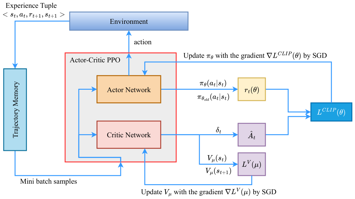
This stochasticity not only facilitates exploration by encouraging the agent to sample diverse actions but also plays a critical role in avoiding premature convergence to suboptimal policies. In high-dimensional action spaces, deterministic policies may struggle to adequately explore the environment, leading to limited learning. By introducing noise proportional to the standard deviation σ ( s t ) , the policy retains flexibility and adaptability, particularly in the early stages of training. Over time, as the policy converges and the variance decreases, the actions become more deterministic, reflecting the agent’s confidence in its learned strategy. This dynamic balance between exploration and exploitation is a hallmark of PPO, making it robust and efficient. The overall training process of PPO is outlined in Figure 1.

2.3. Statistical Time-Domain Features

The statistical time-domain features [1,24] capture statistical characteristics of the vibration signal, providing valuable insights into system health by highlighting changes associated with wear and degradation. Notably, these extracted features often exhibit a positive correlation with the RUL of the component, serving as key HIs of its operational condition. Additionally, the kurtosis feature aids in identifying the first prediction time (FPT), a critical parameter used for generating labels in training RUL estimation models [15].
For RUL estimation, understanding the correlation between predictors and the response variable is crucial for effective modeling. Ideally, features should exhibit a strong correlation with RUL, whether positive or negative. A negative correlation is commonly observed, as many condition-monitoring parameters, such as vibration, increase with machine degradation, leading to lower RUL values. On the other hand, weakly correlated features contribute little to RUL prediction and may introduce noise, reducing the model’s effectiveness. The time-domain features utilized for this study are presented in Table 3.

2.4. Normalized RUL and First Prediction Time

An important aspect of RUL estimation is the labeling process, which is crucial in accurately modeling the degradation of the bearing or gear. In this chapter, a piece-wise linear RUL target function [15] is adopted to create the RUL labels. Conventionally, RUL is assumed to decrease linearly over time; however, this assumption does not align with the actual behavior of most mechanical systems. These mechanical components/systems tend to remain in a healthy state for an initial period before degradation begins. To address this, the piece-wise linear RUL function has been utilized. This function keeps the RUL constant during the healthy phase of operation and then models it as linearly decreasing once degradation begins, at a point known as the FPT. Equation (5) can be used to create the RUL labels. The labeling process focuses more on the data after the FPT, as this is the critical period for RUL prediction. By representing the RUL labels in this piece-wise manner, the function captures the natural progression of degradation more accurately and ensures that predictions are grounded in the actual operational behavior of the bearing.
RUL i = 1 , T i FPT 1 T i FPT T e FPT , T i > FPT
where T i is the current sample and T e is the sample at failure or the final sample.
To determine the FPTs of each bearing, the 3 σ interval method [25] is utilized. The mean and standard deviation of the initial 30 samples of the kurtosis of the x-direction vibration signal are computed to define the 3 σ bounds, with the upper bound as μ + 3 σ and the lower bound as μ 3 σ since kurtosis is the feature that is able to provide most information about incipient faults [15]. i.e., anomalies. Kurtosis is used because of its high sensitivity to impulsive changes in the vibration signal, which are characteristic of early-stage faults. Unlike energy-based features such as RMS or variance that respond significantly only in later stages of degradation, kurtosis can detect small, localized defects—such as micro-cracks or surface pitting—by capturing rare, high-amplitude events in an otherwise steady signal. Since healthy signals typically follow a near-Gaussian distribution with a kurtosis value around 3, any deviation from this indicates a shift in signal behavior due to emerging faults. This makes kurtosis particularly effective for identifying the onset of degradation, enabling timely detection and accurate initiation of the RUL prediction process.
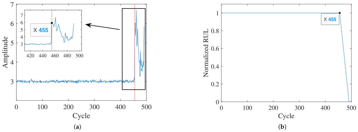
Moving on, the FPT is identified as the first sample where three consecutive points in the data fell outside these bounds, signaling the start of potential degradation. If no such sample satisfies this condition, no FPT is detected based on the 3 σ rule and kurtosis. In such cases, the RMS of the vibration signal is used as an alternative. Three consecutive points are chosen to mitigate the influence of noise, as noise is unlikely to cause such a pattern consistently. This method provides a robust statistical approach for identifying the transition from healthy operation to the degradation phase for components. Figure 2a shows the kurtosis of the raw time-domain signal and the FPT at the 455th time cycle for bearing 2_1, while Figure 2b shows the corresponding RUL labels for that specific bearing.

3. Proposed Method

3.1. Dataset Description

The XJTU-SY Bearing Dataset was generated by Wang et al. [26], which includes the accelerated run-to-failure data of 15 separate rolling element bearings. The dataset contains run-to-failure vibration signals in the x and y directions. The accelerated degradation experiments involved three operating conditions, with five bearings tested under each condition. The operating conditions are 2100 rpm (35 Hz) with 12 kNm load, 2250 rpm (37.5 Hz) with 11 kNm load, and 2400 rpm (40 Hz) with 10 kNm load.
To record the vibration signals of the bearings, two PCB 352C33 accelerometers were installed at 90° angles on the housing of each tested bearing—one positioned along the horizontal axis and the other along the vertical axis. The sampling frequency was set to 25.6 kHz. To ensure the complete degradation process of each bearing was captured (from normal operation to severe fault), the tests continued until the maximum amplitude of either the horizontal or vertical vibration signal exceeded 10× A h , where A h represents the maximum amplitude of the vibration signals during the normal operating stage. For this study, bearing 2_1 will be used, which has a lifetime of 491 min at 2250 rpm and 11 kNm load. The bearing fails with an inner race fault, and there are 491 files in the dataset that contain 32,767 samples of data sampled every 1 min for 1.28 s.

3.2. Data Preprocessing and Feature Extraction

To ensure the reliability and usability of the dataset, data preprocessing was implemented before feature extraction. The preprocessing part for this chapter consisted of z-score normalization. Z-score normalization transforms data to have zero mean and unit variance [1]. It rescales the data so that each feature contributes equally to training of the model, regardless of its original scale.
Following preprocessing, feature extraction was performed to derive meaningful indicators of bearing health. Statistical time-domain statistical features (Table 3) were extracted from the x direction vibration signals of the dataset to capture signal variations indicative of fault progression. The features were extracted for each file in the dataset, making up 491 samples of five features.

3.3. Principal Component Analysis

The five statistical time-domain features defined in Table 3 are not statistically independent. Four of them, namely the maximum value, root mean square, square root mean, and standard deviation, respond directly to the amplitude growth that characterizes bearing degradation, and a degree of inter-correlation in the raw feature set is therefore expected by construction.
To address this, principal component analysis (PCA) [27] is applied to the five normalized time-domain features prior to state construction. PCA performs an orthogonal linear transformation of the feature space such that the resulting components are mutually uncorrelated by construction, with each successive component capturing the largest residual variance subject to orthogonality with all preceding components. Given the centred feature matrix X R n × d with n samples and d = 5 features, PCA produces a transformation matrix W R d × d whose columns are the eigenvectors of the sample covariance matrix 1 n 1 X X , and the transformed representation is given by Z = X W .
In this study, PCA is used for decorrelation rather than for dimensionality reduction. All five principal components are retained, so that the transformation preserves 100% of the variance present in the original five-dimensional feature space and no information is discarded. The resulting state representation is therefore equivalent in information content to the original feature set, but mutually uncorrelated. To preserve the fit between the PCA transformation and the training data, W is fitted on the training partition only and the same transformation is then applied to the test partition, so that no information from the test set leaks into the construction of the input representation. The PPO actor and critic networks, as well as the LSTM and MLP baselines, take the five PCA-transformed components as their input rather than the raw normalized time-domain features.

3.4. State Construction, Action and Reward

3.4.1. State Construction

To construct the states (response and predictors) for the models (PPO uses states, while deep learning models use sequences and machine learning models use samples), the feature set was used in conjunction with the RUL labels generated using the FPT. From the feature set, only the data containing degradation information was included in the training and testing process—specifically, the 10 samples preceding the FPT and all data after the FPT. The sliding-window approach has been applied to transform sequential data (time-domain features) into overlapping segments, enabling the model to learn temporal patterns effectively. In this study, the window size is set to 10, meaning that each window contains data from the past 10 time steps. The stride, set to 1, determines the step size for moving the window across the dataset. Additionally, the horizon is set to 0, ensuring that the target label for each window corresponds to the last step within the window without any look-ahead. This approach maintains alignment between the input states and their associated targets, facilitating accurate predictions while adhering to the sequential nature of the data. It must be noted that the dataset has been split into training and testing sets before applying the sliding window. Specifically, 75% of the data has been used as the training set, while 25% has been used as the testing set.

3.4.2. Action and Reward

The action space for the DRL agent is designed in a manner such that it directly estimates the RUL of the component depending on the states (statistical time-domain features). The PPO framework’s actor network yields a scalar value representing the estimated RUL in the range [ 0 , 1 ] , which serves as the action of the agent for a given state. The reward function is designed to drive the agent to minimize the error between the predicted RUL ( R U L t ^ ) and actual RUL ( R U L t ) at the current state. Specifically, the reward r t at time t is defined in Equation (6).
r t = 1 × ( R U L ^ t R U L t ) 2
A quadratic penalty, which increases with the square of the deviation from a target value, is incorporated into the reward structure. This encourages the agent to make accurate RUL predictions, as large deviations from the actual RUL result in significantly greater negative rewards, driving the policy to iteratively refine its predictions. Small errors are penalized lightly because the square of a small error results in an even smaller value, maximizing the reward. In contrast, large errors are penalized heavily, as the square of a large error amplifies its magnitude, minimizing the reward.
It is worth clarifying the conceptual character of the MDP formulation adopted here, since the agent’s action—a scalar RUL prediction—does not physically alter the bearing’s degradation trajectory. In a strict MDP sense, the action therefore does not influence the subsequent state, and the formulation can be described as a “prediction-as-action” adaptation of reinforcement learning to a prognostics setting rather than a canonical control problem in which the agent steers the environment. This conceptual point is acknowledged explicitly. The same formulation has, however, been adopted in a substantial body of recent DRL-for-RUL studies, most directly by Hu et al. [12] and Zheng et al. [15], both of which treat the predicted RUL as the agent’s action and define the reward as a function of prediction error. The framework presented in this study is therefore consistent with this established line of research, and its purpose is to investigate whether the on-policy clipped-objective formulation of PPO offers practical benefits in this setting, rather than to claim a canonical control-theoretic MDP.
Although the reward of Equation (6) superficially resembles a regression loss, the optimization performed by PPO is not equivalent to standard supervised regression on the same target. Three structural differences are worth highlighting. First, the actor parameterizes a stochastic Gaussian policy rather than emitting a deterministic prediction; actions are sampled at training time, and the gradient is taken with respect to the log-likelihood of the sampled action weighted by the advantage. The presence of an explicit entropy term (with coefficient 0.01 in the configuration adopted here) further regularizes the policy in a way that has no analogue in deterministic MSE minimization. Second, the clipped surrogate objective imposes a trust-region constraint on each policy update, bounding the magnitude of parameter changes per iteration; this is structurally distinct from unconstrained gradient descent on MSE and is closer in spirit to natural-gradient and trust-region methods, which are known to produce different optimization trajectories and different generalization behavior. Third, the actor is not updated using raw prediction errors but using advantage estimates produced by the critic, which learns a value function that aggregates the reward signal across the trajectory through the discount factor γ and the GAE parameter λ . The training signal seen by the actor is therefore a temporally smoothed quantity rather than a per-sample error term. Empirically, the consequences of these structural differences are visible in the results reported in further sections the MLP, trained with standard supervised backpropagation on identical features, shows a pronounced train–test gap (train Score 0.1152 versus test Score 0.5850), whereas PPO does not (train Score 0.2002 versus test Score 0.0512). Were the two formulations mathematically equivalent on this task, such a train-test difference would not be expected.

3.5. Model Selection and Training

In this chapter, three different RUL estimation models—LSTM, MLP, and PPO—are trained and evaluated for RUL estimation of the bearing. The choice of these three models reflects the scope of this study, which is to investigate whether an on-policy clipped-objective DRL formulation (PPO) offers practical benefits for bearing RUL estimation relative to supervised counterparts trained on the same statistical time-domain features. The two supervised baselines are therefore selected to share the input representation used by the PPO actor and to span a representative range of supervised behaviors: a feedforward static-feature regressor (MLP) and a sequential temporal regressor (LSTM). A more detailed justification for this baseline selection—including why off-policy DRL methods and advanced sequence backbones such as TCNs and Transformers are not included here—is provided below. The rationale behind each of the three models is given next.

3.5.1. LSTM Model

LSTMs are designed to handle sequential dependencies, making them well-suited for RUL estimation, where past machine conditions influence future degradation states. Since the dataset consists of manually extracted time-domain features, the LSTM model leverages its ability to process sequential inputs and recognize long-term dependencies within the vibration data. The gated architecture of LSTMs ensures efficient learning of degradation trends while mitigating vanishing gradient issues.

3.5.2. MLP Model

An MLP model is included as a baseline to assess the effectiveness of sequential deep learning models compared to a traditional feedforward neural network. Although MLPs do not inherently capture temporal dependencies, they can still learn complex nonlinear relationships between the extracted time-domain features and RUL labels. This comparison helps determine whether explicitly modeling temporal relationships provides a significant advantage over static feature-based models.

3.5.3. PPO Model

In addition to supervised learning models, an RL-based approach using PPO with MLP is explored. Since the dataset consists of manually extracted features, this model treats RUL estimation as a sequential decision-making process, optimizing a policy to predict RUL dynamically. Unlike traditional supervised models that directly minimize prediction error, the PPO-based model leverages reward functions to improve long-term prediction accuracy and robustness to uncertainties in machine degradation.

3.5.4. Training Process

The training process for the LSTM and MLP models was fairly simple, as they were trained using supervised learning, where the models learned to map extracted features to the RUL labels by minimizing a loss function (RMSE). The LSTM model processed sequential input data, capturing long-term dependencies through recurrent connections and updating weights via gradient descent. The MLP learned nonlinear relationships between the manually extracted time-domain features and RUL values through multiple hidden layers using activation functions and backpropagation.
The training process for the PPO algorithm involved several carefully designed steps to optimize both the actor and critic networks while adhering to the constraints of PPO. These steps were aimed at enabling the agent to learn an optimal policy for predicting RUL based on the provided input data. At the start of each episode, a batch of sequential data was sampled from the training dataset (states). The batch size was predefined to ensure that the agent learned from diverse segments of the data in each episode. Each sampled segment consisted of state inputs (features representing time-domain data) and corresponding RUL targets. These states were fed into the actor–critic model to generate actions and associated log probabilities, which represented the policy’s predictions for the RUL. The sampled RUL targets were then used to compute the reward signal for the agent.
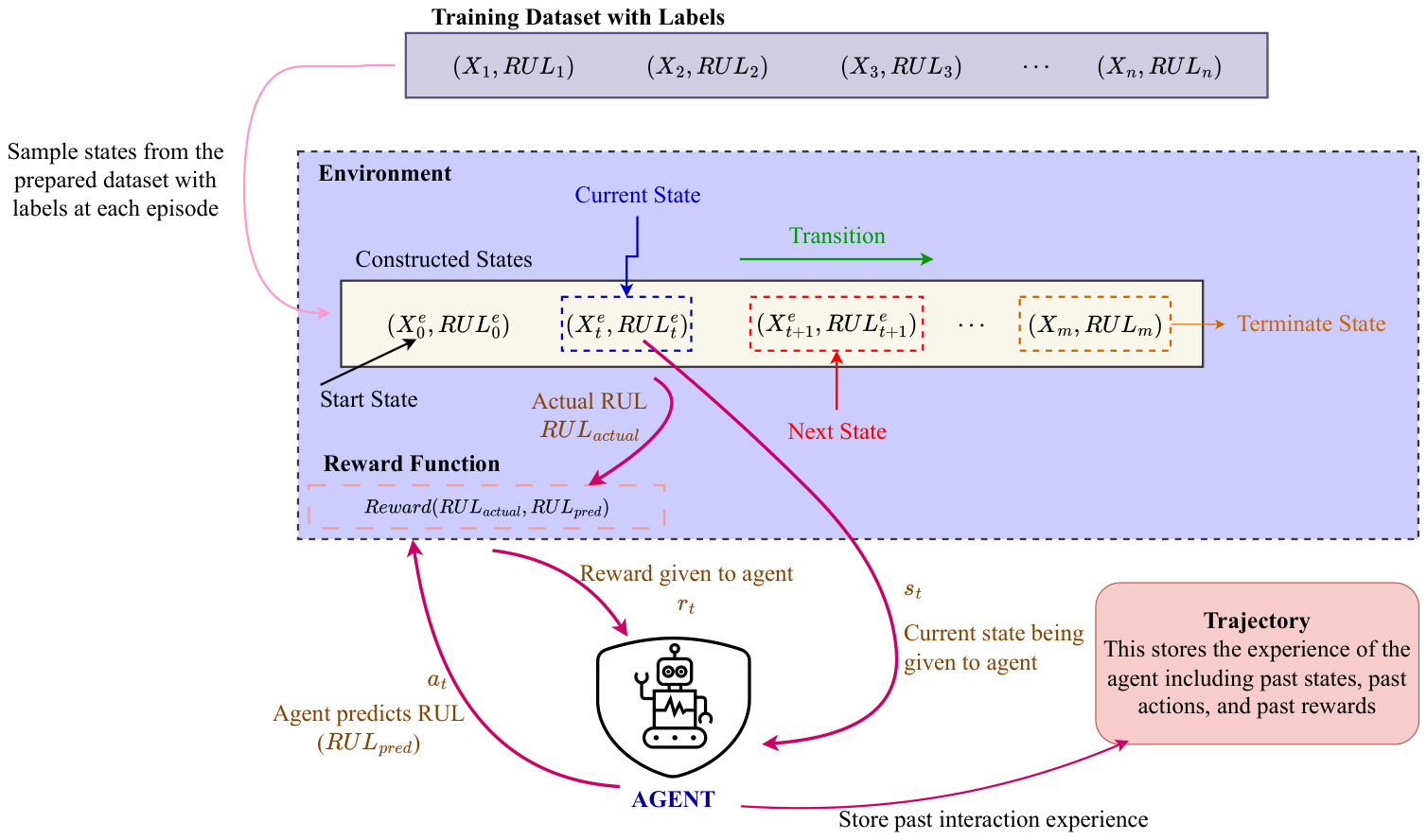
The actor network of the PPO agent then predicted a probability distribution over possible actions, parameterized by a mean and standard deviation. Using this distribution, an action was sampled, and its log probability was calculated. Simultaneously, the critic network evaluated the current state to estimate its value. The reward for each action was computed as the negative squared error between the predicted RUL (action) and the true RUL (Equation (6)). This reward design encouraged the agent to minimize prediction error over time. The agent stored transitions—states, actions, log probabilities, rewards, and done flags—in a memory buffer used for policy updates. At the end of each episode, it computed advantages and returns from this memory. PPO used generalized advantage estimation (GAE) to compute advantages, balancing short- and long-term rewards. These were normalized to stabilize training. The actor was updated using a clipped surrogate objective to limit drastic policy changes, while the critic minimized MSE loss between predicted and actual returns. Both networks were trained over multiple epochs to refine the policy and value estimates. The constructed environment and the agent interaction procedure with the environment are outlined in Figure 3.

3.5.5. Rationale for Baseline Selection

The baselines adopted in this study, namely LSTM and MLP, are chosen to isolate the contribution of the learning paradigm rather than the contribution of the backbone architecture. Two alternative classes of comparison could in principle be included: off-policy continuous-action DRL methods (such as DDPG, SAC, and TD3) and advanced temporal architectures (such as Temporal Convolutional Networks (TCNs) and Transformers). Neither is included here for the reasons set out below.
The contribution of this study is to validate PPO, an on-policy clipped-objective method, as a viable alternative to the deterministic off-policy actor–critic methods (predominantly DDPG and TD3) that currently dominate the DRL-for-RUL literature. The relevant comparison for this contribution is therefore between PPO and supervised baselines that share its feature backbone, which is what is provided here. A controlled head-to-head comparison between PPO and an off-policy DRL method such as DDPG or SAC is itself a substantial undertaking: it requires careful matching of state definitions, replay-buffer configuration, exploration schedule, target-network update frequency, and learning-rate schedules across two structurally distinct algorithm families. Such a study warrants dedicated treatment rather than being appended to a proof-of-concept investigation, and it is explicitly listed as future work. The qualitative comparison of PPO against DDPG, SAC, TD3, TRPO, and DQN provided in Table 2 identifies PPO’s stability under limited and noisy degradation trajectories, conditions that are characteristic of run-to-failure datasets, as the principal motivation for its selection over deterministic off-policy alternatives, whose sensitivity to hyperparameter tuning and known instability on small datasets are well documented in the DRL literature.
TCNs and Transformers are increasingly used in time-series prognostics and would, in isolation, constitute reasonable comparison points for a study whose objective is to benchmark backbone architectures. The objective of this study, however, is different: it is to compare learning paradigms (reinforcement learning versus supervised learning) under a common feature representation. Introducing a TCN or Transformer supervised baseline would conflate two separate questions: (i) does the PPO learning paradigm offer benefits over supervised regression, and (ii) does a larger or more modern backbone offer benefits over a smaller one? These are distinct research questions, and answering the second does not advance the first. Furthermore, the PPO actor used in this study is itself an MLP. Comparing a PPO-MLP against a supervised Transformer would no longer test whether the PPO paradigm offers benefits over supervised learning; it would test whether a small MLP trained under PPO can match a large Transformer trained under supervised learning, which mixes the paradigm and the backbone in a way that is not informative for the question of interest. The supervised baselines are therefore restricted to MLP and LSTM so that the backbone capacity is comparable to the PPO actor and the paradigm comparison is clean. A naive linear regression baseline is additionally included to verify that the test task is not trivially solvable by extrapolation of the RUL label trend. Comparison against advanced temporal architectures, with controlled backbone capacity across the supervised and reinforcement-learning conditions, is identified as future work.

3.5.6. Evaluation

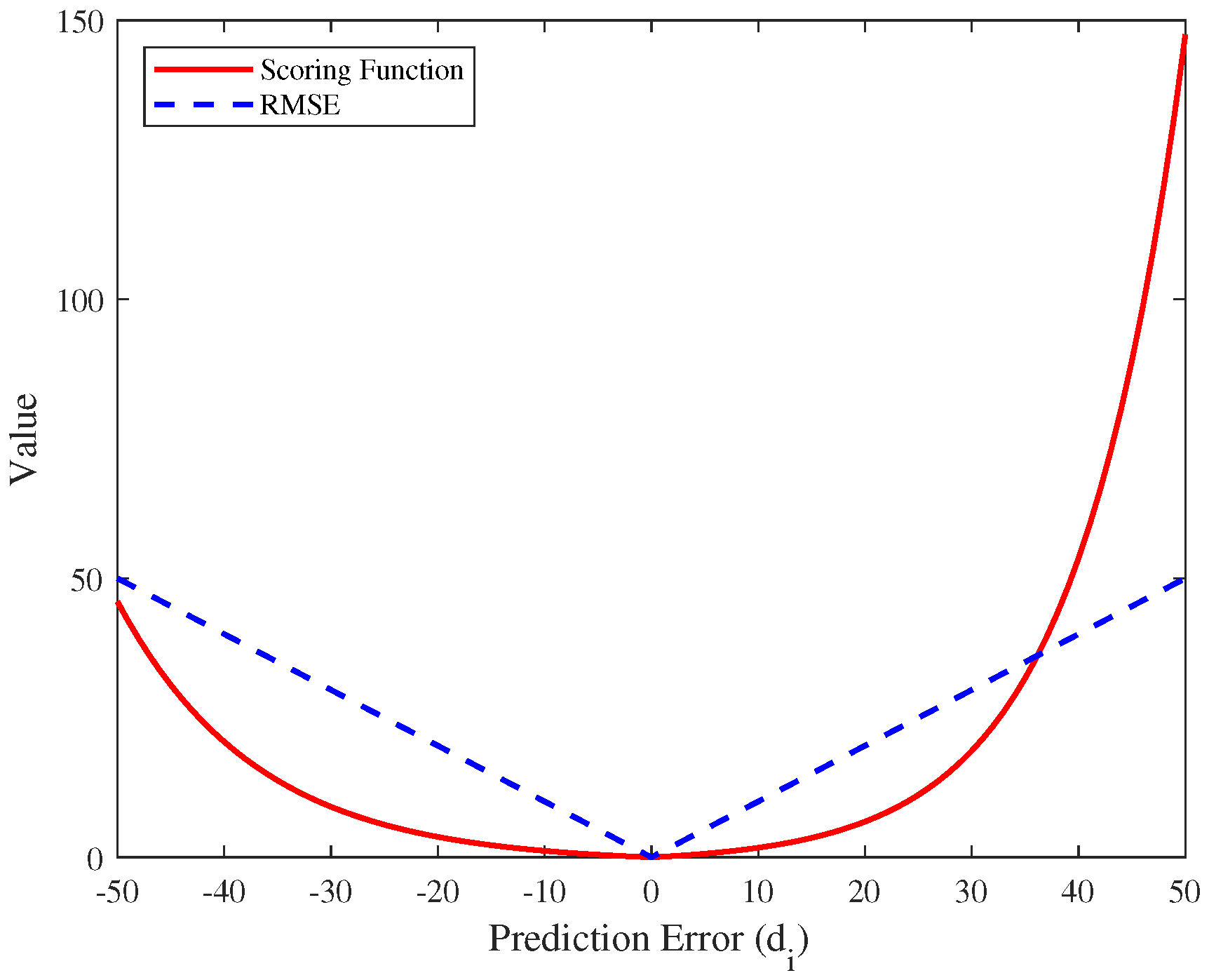
To evaluate the performance of the proposed approach, two prominently used metrics have been used. These are the RMSE provided in Equation (7) and the scoring function provided in Equation (8). RMSE is a standard metric used to evaluate the accuracy of predictions. It calculates the square root of the average squared differences between predicted and actual values, providing a measure of the average magnitude of prediction errors. In this chapter, RMSE is used to assess the deviation of predicted RULs from the true RULs. The scoring function is a custom-designed metric that penalizes late predictions more severely than early ones (i.e., when the estimated RUL exceeds the actual RUL). By contrast, RMSE treats late and early estimations equally. This reflects the higher risks associated with unexpected failures in industrial scenarios, where late predictions can lead to significant disruptions.
R M S E = 1 n i = 1 n d i 2
s c o r e = i = 1 n e d i 13 1 if d i < 0 , e d i 10 1 if d i 0 .
where n is the number of testing samples and d i = R U L i ^ R U L i is the error between the actual and predicted RUL at the ith testing sample. The difference between the evaluation metrics is portrayed in Figure 4.

4. Results and Discussion

4.1. Feature Set Exploration

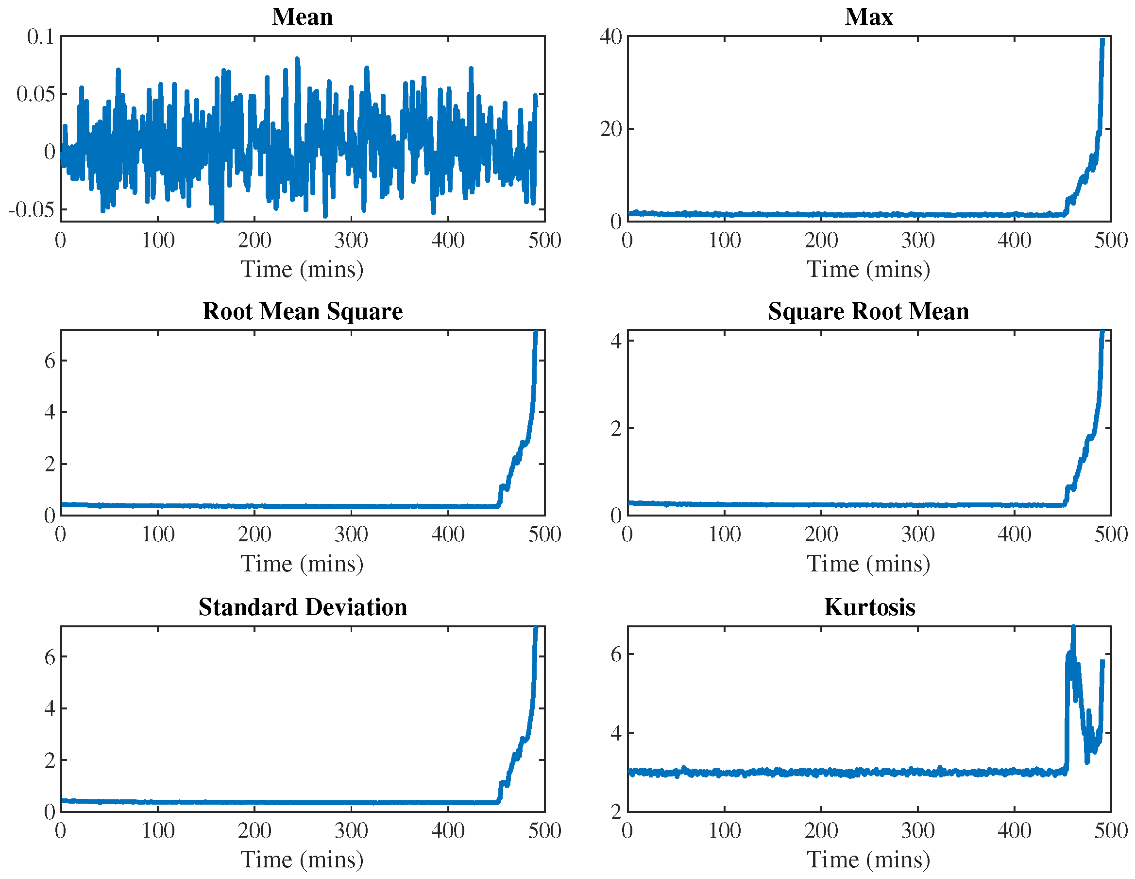
Figure 5 shows the time-domain features, which were extracted from the raw x direction vibration signals of bearing 2_1. It can be seen that the features’ max, root mean square, square root mean, and standard deviation show an increasing trend as the time to failure approaches. The failure time for bearing 2_1 was 491 min. This is indicative of the fact that as failure approaches, the vibration emanating from the component starts to increase. These features show a steady trend during the early stages of the bearing life, followed by a steep, exponential-like rise at approximately the 455th minute as the bearing approaches failure. This sudden increase is indicative of the emergence of severe localized defects, leading to large amplitudes in the vibration signal. The mean values remain centered around zero with minor fluctuations, indicating that the signal maintains zero-centered behavior throughout the majority of its life cycle, suggesting a balanced vibration response. The kurtosis, a statistical measure of peak sharpness and impulsiveness, remains relatively constant in the healthy operating region but shows a significant increase shortly before failure. This elevation suggests the presence of impulsive events typical of defect growth, such as spalling or pitting in the bearing surface. The kurtosis feature has been used to determine the FPT of the bearing in this study. Collectively, the evolution of these features demonstrated a clear correlation between signal amplitude statistics and bearing degradation. The relatively constant behavior during the early operational phase provided a baseline reference, while the late-stage divergence of the features served as a strong indicator of imminent failure. These observations indicated that features such as Max, RMS, SRM, and σ (standard deviation) were highly sensitive to bearing degradation and could be effectively utilized as health indicators in this study.
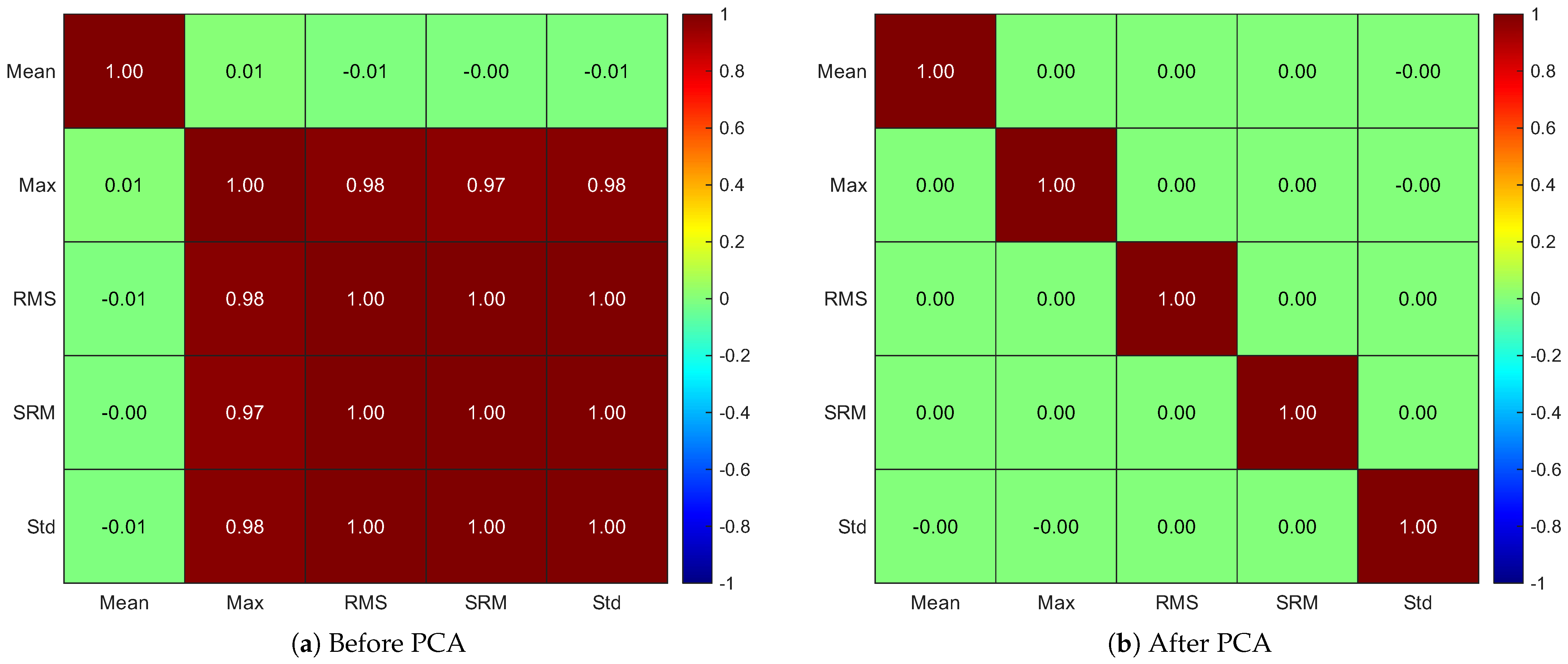
The correlation of these features is tested before training the models. Figure 6a shows the correlation matrix of the five time-domain features (mean, Max, RMS, SRM, and Std) of bearing 2_1 after z-score normalization. The matrix reveals near-perfect mutual correlations (approximately 0.97 to 1.00) among Max, RMS, SRM, and Std, which is expected given that all four features respond directly to the amplitude growth that characterizes bearing degradation. By contrast, the mean feature is essentially uncorrelated with the other four (absolute correlations below 0.02), consistent with its zero-centred behavior throughout the bearing’s life, as shown in Figure 5. The redundancy among the amplitude-based features confirms that the raw state representation contains a high degree of linear dependence, motivating the application of PCA to obtain a decorrelated representation prior to state construction. This redundancy, if left untreated, would supply the learning models with effectively repeated information and could produce ill-conditioned input geometry during gradient-based optimization.
Figure 6b shows the correlation matrix of the five principal components obtained by applying PCA to the five time-domain features. All off-diagonal entries are reduced to zero up to numerical precision, confirming that the PCA transformation has successfully eliminated the linear dependence observed among the features in Figure 6a. The five resulting principal components therefore form a decorrelated basis that spans the same five-dimensional feature space as the original representation, with no loss of information since all five components are retained. This decorrelated representation is the actual input supplied to the PPO, LSTM, and MLP models in Section 4.2.

4.2. Model Architecture

4.2.1. PPO

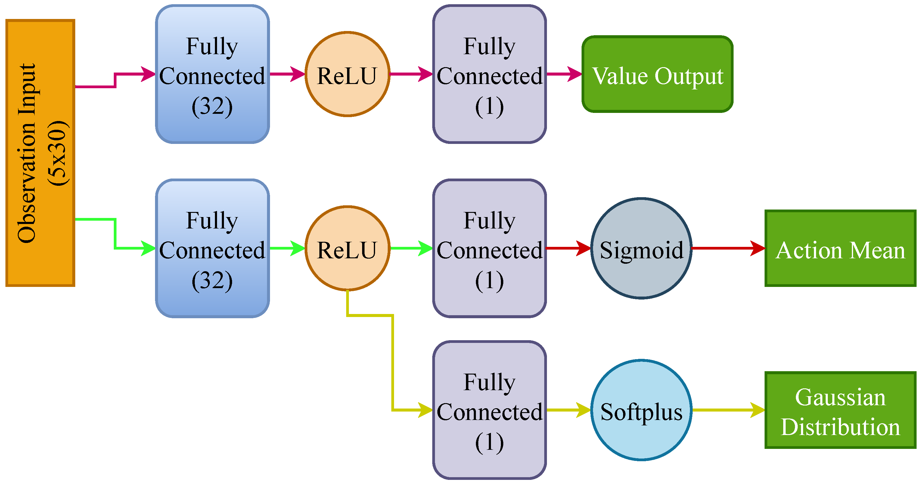
The architecture of the PPO model is outlined in Table 4 and Figure 7. It uses an MLP network to form its actor and critic network architecture employed in the RUL estimation framework. Both networks share a common input dimension of 5 and utilize a single hidden layer comprising 32 neurons activated by the ReLU function. The actor network is designed to output the parameters of a Gaussian distribution, specifically the mean and standard deviation, which are used to model the policy. To ensure appropriate scaling, the mean is passed through a Sigmoid activation function, constraining it within a bounded range, while the standard deviation is passed through a Softplus activation to guarantee non-negativity. In contrast, the critic network outputs a single scalar value representing the estimated value function V ( s ) , indicating the expected return from a given state. This output does not employ any activation function, allowing it to freely represent both positive and negative value estimates. The architectural symmetry in the hidden layers of both networks promotes consistency, while their distinct output configurations reflect their specialized roles in the actor–critic paradigm.
Table 5 presents the parameters used for training the PPO algorithm. The model was trained for 8000 episodes using a discount factor of 0.99, which ensures future rewards are considered while still prioritizing immediate gains. GAE was applied with a lambda value of 0.95 to balance bias and variance in advantage estimation. A clipping ratio of 0.2 was used to constrain policy updates within a safe range, enhancing stability. Both the actor and critic networks were optimized using the Adam optimizer, with learning rates of 5 × 10 4 and 1 × 10 3 , respectively. Training was conducted in mini-batches of size 32, with experience samples collected in a buffer of size 2000. Each policy update was run for 10 epochs. An entropy coefficient of 0.01 was included to encourage exploration by penalizing overly confident action distributions. These hyperparameters collectively promote stable and efficient policy learning.
4.2.2. LSTM

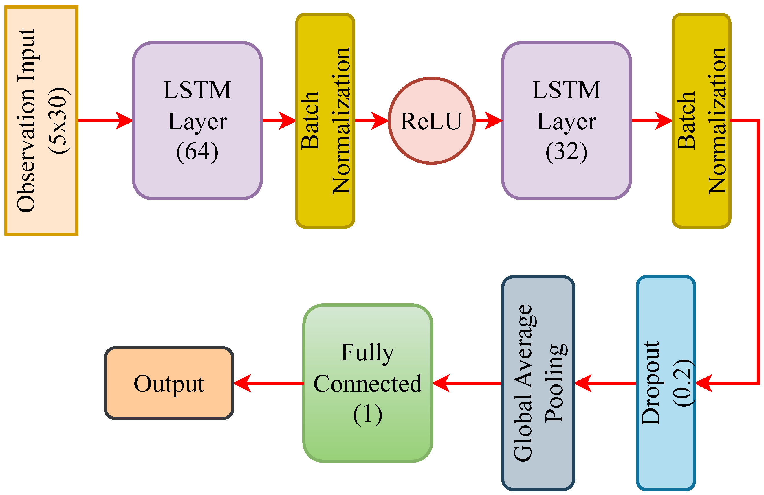
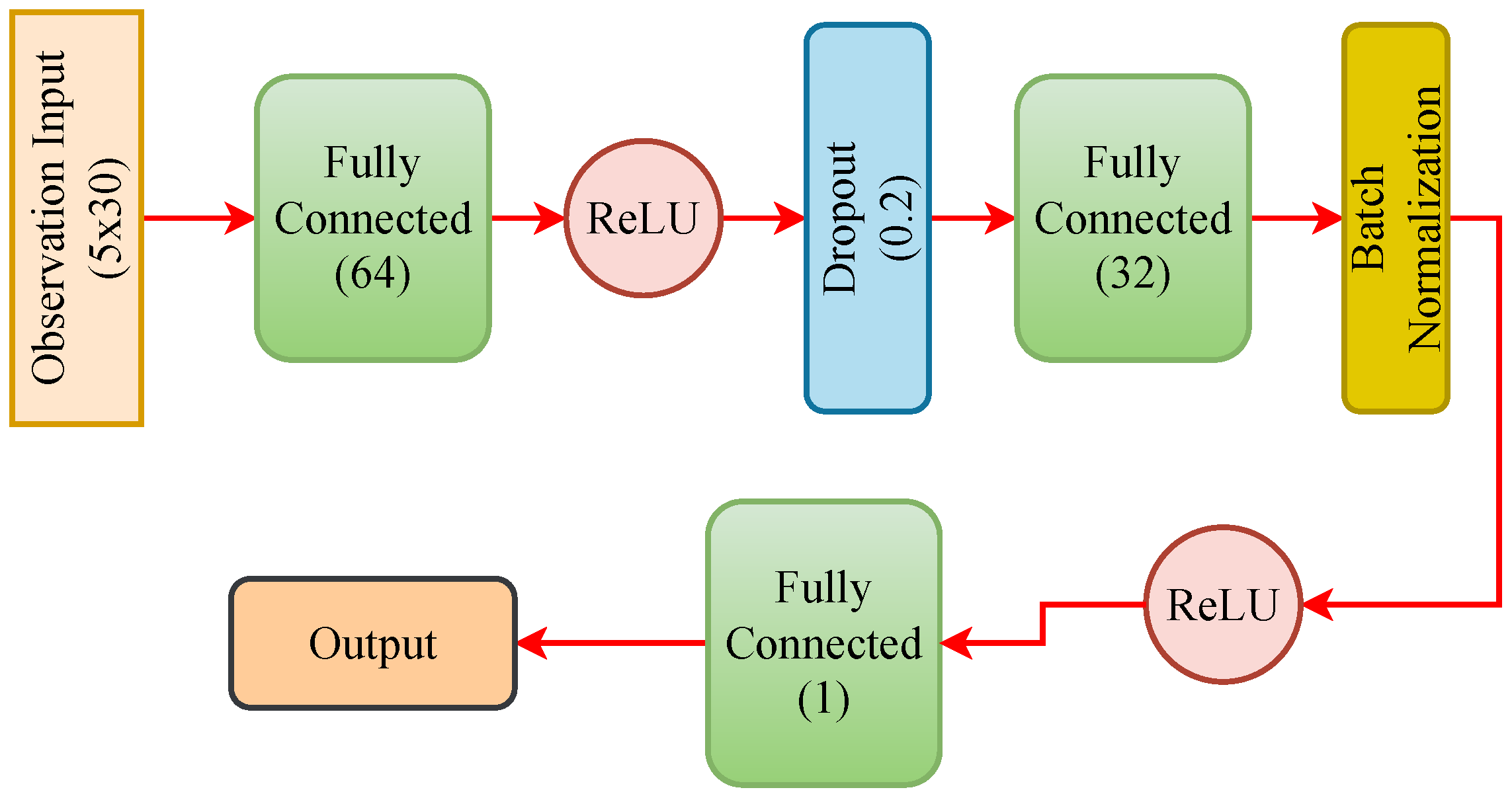
The proposed LSTM model (Figure 8 and Table 6) for bearing prognostics takes an observation of size 5 × 30 (five features over 30 time steps) and estimates a single scalar corresponding to the bearing’s RUL by learning temporal degradation patterns with stacked LSTM layers. Specifically, the input sequence is processed by an LSTM layer with 64 hidden units, whose outputs are batch-normalized to stabilize and accelerate training, then passed through an ReLU nonlinearity to increase representational capacity for nonlinear degradation behavior. A second LSTM layer with 32 hidden units further refines the temporal representation and is again followed by batch normalization to maintain well-conditioned intermediate activations during optimization. To reduce overfitting, a dropout rate of 0.2 is applied after the recurrent stack, and global average pooling aggregates the sequence-level information into a fixed-length descriptor by averaging across the temporal dimension. Finally, a fully connected layer with one neuron produces the RUL estimate using a linear output.

4.2.3. MLP

Table 7 and Figure 9 outline the architecture of the MLP network designed for RUL estimation. Concretely, the model accepts time-domain features and first projects them through a dense layer with 64 hidden units, followed by an ReLU activation to introduce nonlinearity and improve the representational capacity of the network. To mitigate overfitting and encourage robust learning from run-to-failure data, a dropout layer (rate = 0.2) is applied during training, which randomly deactivates a subset of hidden units and reduces co-adaptation among learned features. The resulting latent representation is then refined by a second dense layer with 32 hidden units and batch normalization, which normalizes intermediate activations across mini-batches to stabilize optimization and improve training efficiency. A second ReLU activation follows to preserve nonlinearity, and the network terminates with a final dense layer of size 1, producing a scalar RUL prediction for the bearing at the current observation.

4.3. PPO Training

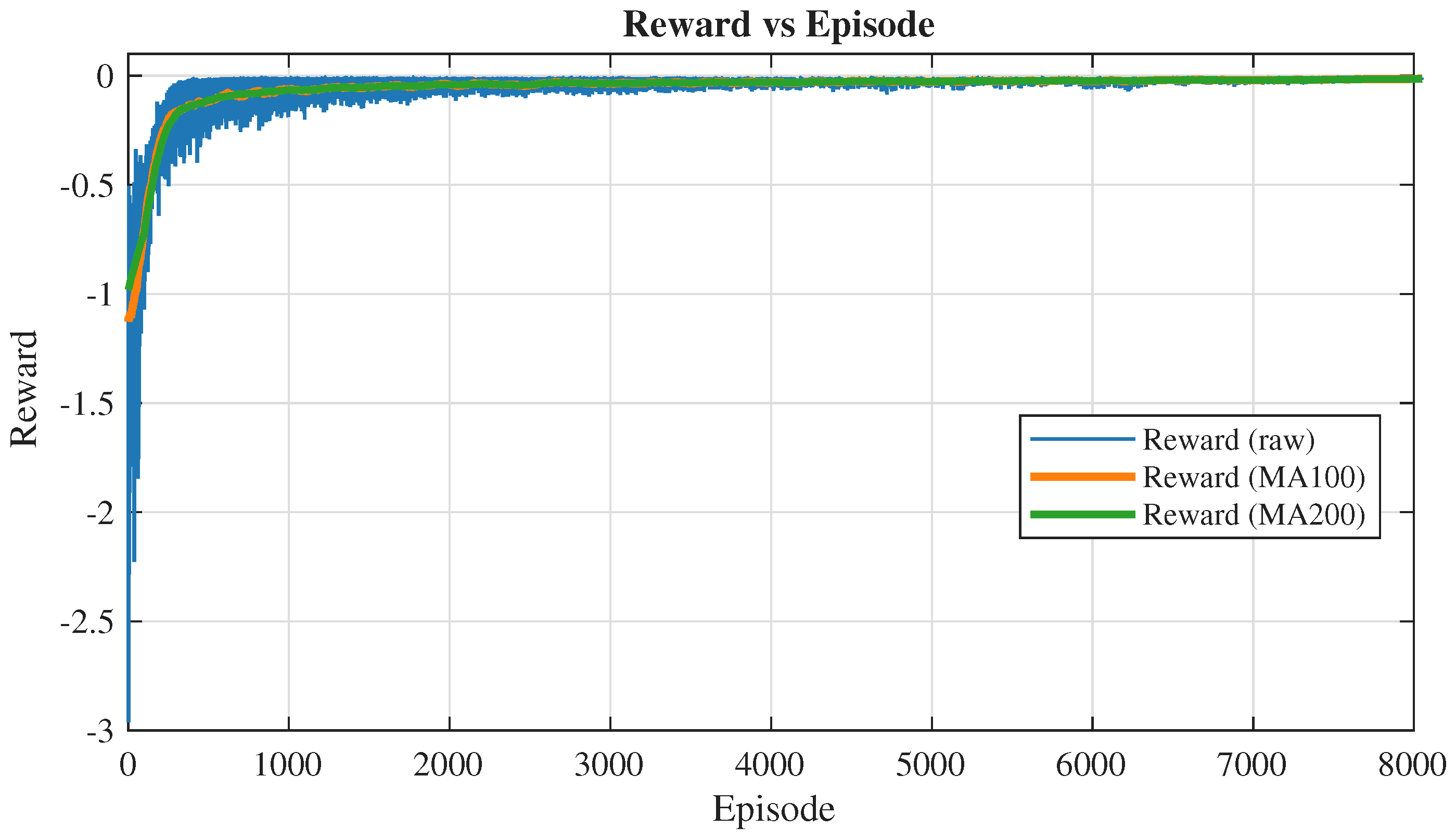
The reward curves presented in Figure 10 and Figure 11 provide important insight into how the PPO agent learns to estimate the RUL over the course of training. Because the reward is defined as the negative squared difference between the predicted and actual RUL values, the large negative reward values observed in the early episodes indicate that the agent initially makes highly inaccurate predictions. This behavior is expected, as the actor and critic networks begin with randomly initialized weights, and the stochastic Gaussian policy encourages wide exploration during the initial learning phase. The resulting high-variance predictions cause fluctuating and strongly negative rewards, reflecting the agent’s lack of understanding of the underlying degradation patterns in the early part of training.
As training progresses, both the raw and moving-average (100-episode and 200-episode windows) reward (see Figure 10 and Figure 11, plot legends) curves begin trending upward toward zero, indicating a reduction in prediction error. This improvement reflects the stabilizing influence of PPO’s clipped objective and the more accurate value estimates produced by the critic network. GAE further contributes to this stability by reducing variance in advantage calculations, enabling more efficient and consistent updates to the actor network. During this middle segment of training, the agent gradually shifts from broad exploratory behavior to more structured predictions that better capture the relationship between time-domain statistical features and the corresponding RUL labels. The smoothing of the moving-average curves illustrates that the agent’s predictions become more consistent, with fewer large deviations from the true RUL.
The last 2000 episodes (Figure 11) show the reward curve narrowing into a relatively stable band very close to zero. This indicates that the policy has largely converged, and the agent is consistently producing low-error RUL estimates. While minor fluctuations persist due to the stochastic nature of the Gaussian policy and the inherent variability in degradation data, the overall stability demonstrates that the PPO agent has successfully learned a reliable policy for mapping input feature states to accurate RUL predictions. Interpreted within the context of RUL estimation, the upward movement and stabilization of the reward curves confirm that the PPO-based model improves its predictive accuracy over time and performs particularly well during the critical late-degradation phase where accurate RUL predictions are most essential.
The actor loss curve in Figure 12 shows how the PPO policy becomes more stable over training. Initially, the loss is high and oscillatory due to random network initialization, noisy advantage estimates, and broad exploration from the stochastic Gaussian policy. As training progresses, PPO’s clipping mechanism and increasingly accurate value estimates lead to smoother, smaller updates, causing the actor loss to decrease and stabilize. In the later stages, the loss settles into a narrow range with only minor fluctuations—expected due to stochastic action sampling and entropy-driven exploration—indicating that the policy has largely converged and is undergoing only small refinements. The absence of sharp spikes or divergence confirms that the selected hyperparameters support stable and controlled policy optimization.
The critic loss curve in Figure 12 shows how the value network improves its ability to approximate the expected return V(s) throughout training. Initially, the critic loss is high and unstable because the value function is poorly estimated due to untrained weights and inconsistent reward signals arising from inaccurate early RUL predictions. As the agent gathers more experience and its predictions improve, the critic receives more reliable learning targets, leading to a clear downward trend and a smoother loss curve that reflects increasingly accurate value estimates. In the later stages of training, the critic loss stabilizes at a lower level, indicating convergence of the value function and the provision of consistent advantage estimates, which in turn support more stable policy updates. Although minor fluctuations persist—due to ongoing policy evolution and stochastic mini-batch optimization—the overall reduction and stabilization of critic loss confirm that the actor–critic process is functioning as intended and that the critic is effectively guiding the PPO agent toward more accurate RUL predictions.
Table 8 summarizes the RUL estimation performance of the proposed PPO-based approach against two supervised baselines (LSTM and MLP) and a naive linear regression baseline, using four metrics: an asymmetric prognostics score, MAE, RMSE, and MSE. In this context, lower values indicate better performance for all reported metrics. The score metric is particularly informative for prognostics because it penalizes late predictions more strongly than early predictions, reflecting the higher operational risk associated with underestimating the RUL.
On the training set, the MLP achieves the smallest errors (MAE = 0.0349, RMSE = 0.0460, MSE = 0.0021) and the lowest score (0.1152), showing a very close fit to the training data. However, this advantage does not translate to the test set, where the MLP performance degrades substantially (score = 0.5850, MAE = 0.1575, RMSE = 0.0941). This widening train–test gap suggests that the MLP is more prone to overfitting or is less robust to shifts in degradation trajectories. In contrast, the LSTM exhibits a more consistent generalization pattern: while its training errors are moderate (MAE = 0.0455, RMSE = 0.0694, score = 0.1894), its test results remain in a comparable range (Score = 0.1985), implying improved stability relative to the MLP, though with noticeably larger absolute test errors (MAE = 0.1194) than PPO.
Most importantly, the PPO method provides the best overall test performance across all reported metrics, achieving the lowest score (0.0512) and the smallest errors (MAE = 0.0526, RMSE = 0.0694, MSE = 0.0048). Given the asymmetric nature of the score, this result indicates that PPO not only reduces average error but also better avoids high-cost late predictions, which are critical in maintenance decision-making. The relatively strong test performance of PPO compared with its training metrics further suggests that the learned policy captures a degradation-relevant structure that generalizes beyond the training runs, leading to more reliable RUL estimates under unseen conditions.
A naive linear regression baseline that fits a straight line to the training segment RUL labels and extrapolates it across the test segment is also included in Table 8. It achieves a test score (0.1172) lower than both the LSTM (0.1985) and the MLP (0.5850), and it is outperformed only by PPO (0.0512). This serves both as a sanity check that the test segment is not trivially solvable by trend continuation alone (since PPO is clearly better) and as an additional indicator that the LSTM and MLP fail to extract useful predictive structure from the vibration features available to them.

RUL Prediction Comparison

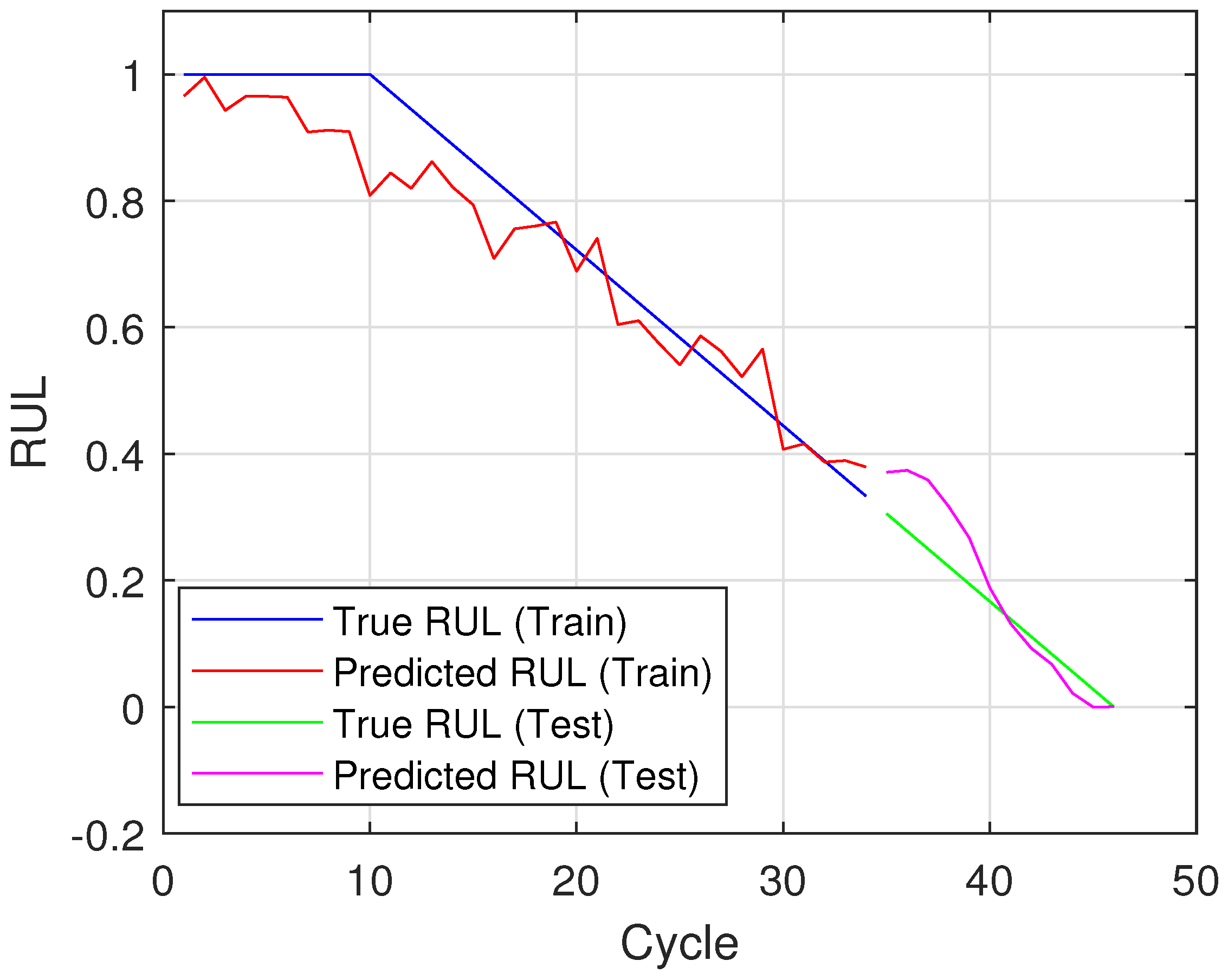
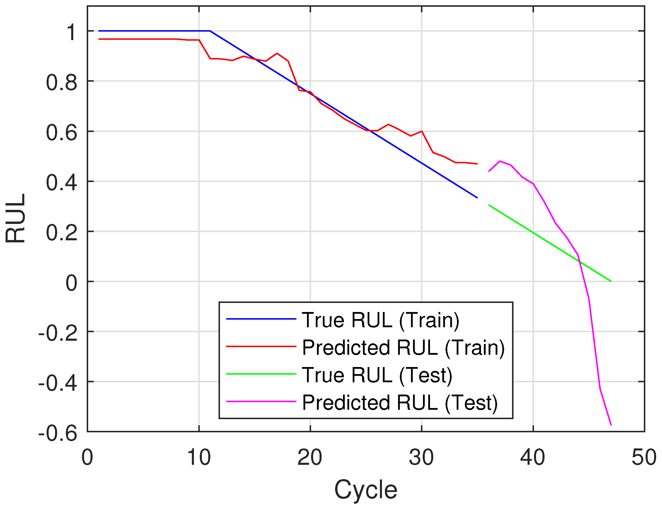
The plot in Figure 13 shows the RUL predictions over operational cycles for both training and testing datasets using PPO. The blue and green lines represent the true RUL for the training and testing sets, respectively, while the red and magenta lines indicate the corresponding predicted RUL. The model demonstrates good tracking performance, accurately capturing the degradation trend in both phases. During the training phase, there are some fluctuations in the early stages (from cycle 0 to 20); however, the model aligns well with the expected RUL values in the later stages. A similar trend is observed during testing, where the predicted values deviate from the true RUL in the early cycles but become more accurate in the later stages. This indicates that the PPO model performs well where it matters most—towards the end of the bearing’s life. Notably, the predicted RUL closely follows the true RUL during the critical degradation region, highlighting the model’s strong learning capability for RUL estimation on this trajectory.
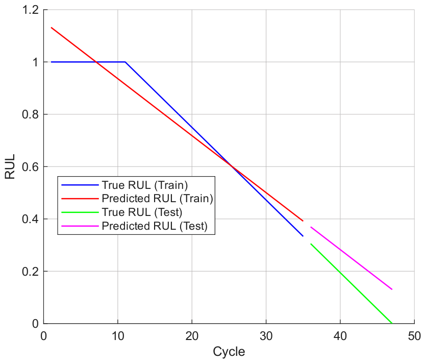
Figure 14 shows the naive linear regression model, which fits a single straight line to the training segment RUL labels and extrapolates it across the test segment without using any vibration-derived features. During training (cycles 1–35), the fitted line passes through the piece-wise linear RUL labels with a clear systematic bias: the line overshoots the constant healthy phase (where the true RUL is held at 1) during the first ten cycles and undershoots the subsequent linearly decreasing region, reflecting the fundamental inability of a single linear fit to capture the piece-wise structure of the RUL target. During testing (cycles 36–47), the extrapolated line continues the same downward trend, but diverges from the true RUL near the end of life, where the model underestimates the remaining life. Quantitatively, the test score (0.1172), MAE (0.0971), RMSE (0.0993), and MSE (0.0099) are all substantially worse than those of PPO. The linear baseline therefore confirms that the chronological test segment is not solvable by the trivial trend continuation of the RUL label, and that the test performance of the learned PPO policy reflects information captured from the vibration-derived features rather than mathematical extrapolation of the label function. Interestingly, the linear baseline outperforms both the LSTM and the MLP on the asymmetric score metric despite using no vibration features at all, which further highlights the failure modes of the supervised baselines on this test segment.
Figure 15 shows that the LSTM captures the overall RUL degradation trend in both training and testing phases, including the initial near-constant phase followed by a monotonic decline. During training, the prediction normally tracks the true curve but exhibits a notable deviation around the degradation onset (change point), where it drops faster before re-aligning with the true RUL. In the test segment, the model preserves the downward trajectory yet becomes optimistic near the end-of-life, tending to overestimate RUL relative to the ground truth. This suggests that while recurrent memory helps smooth predictions and maintain continuity across cycles for LSTM, the model may under-represent late-stage degradation acceleration, resulting in reduced end-of-life accuracy—an important prognostic limitation because late-life errors can be operationally critical when maintenance decisions depend on accurately detecting imminent failure.
Figure 16 indicates that the MLP can approximate the decreasing RUL trend during training but struggles to maintain physically consistent, stable behavior when extrapolating to the test segment. During training, the predicted RUL (red) generally tracks the true RUL (blue) with small oscillations, indicating that the network has learned an average mapping from features to RUL; however, the prediction shows little fluctuations and slight bias around the mid-life region, suggesting sensitivity to short-term variations rather than a smooth degradation progression. In the test region, the predicted RUL (magenta) deviates markedly, exhibiting a delayed/optimistic plateau followed by an abrupt collapse to unrealistic negative RUL values near the end of the trajectory. This sharp drop indicates unstable extrapolation, which is consistent with the limitation of feedforward MLPs for sequential degradation processes: without explicit temporal memory, the model may fit training patterns well, yet fail to capture the underlying time-dependent degradation dynamics, leading to amplified errors—especially near the end of life, where small feature mismatches can cause disproportionately large prediction shifts.
Overall, the PPO-based predictor demonstrates the most operationally relevant accuracy on the test segment of Bearing 2_1 compared with the LSTM, MLP, and naive linear regression baselines, primarily because it maintains close agreement with the true RUL in the critical late-life degradation region where maintenance decisions are most sensitive. While the LSTM captures the global trend, it shows a pronounced change-point deviation and becomes optimistic near the end of life (overestimation), which is undesirable; the MLP exhibits the weakest behavior, with unstable extrapolation on the test trajectory (including unrealistic negative RUL), indicating poor temporal consistency on unseen cycles. The naive linear regression baseline, while structurally limited by its inability to use vibration-derived features, nonetheless outperforms both the LSTM and the MLP on the asymmetric score, which further highlights the failure modes of the supervised baselines on this test segment. In contrast, PPO tracks the degradation trajectory with tighter alignment toward the end of life and avoids the severe end-of-life failure modes observed in the MLP and the late-life optimism observed in the LSTM, which is consistent with its superior test-set performance in Table 8 (lowest score and lower absolute errors). Importantly, this advantage is reinforced by the asymmetric prognostics score, which penalizes late predictions more heavily than early ones; PPO’s lower score therefore indicates not only smaller average error but also fewer high-risk underestimation/overestimation behaviors in the region where prediction mistakes are most costly.
It is worth addressing here whether the chronological train/test split, in which the test segment corresponds to the late-degradation portion of the trajectory, could allow a model to succeed simply by extrapolating the piece-wise linear shape of the RUL labels rather than by learning a meaningful mapping from the vibration-derived features to RUL. If the test set performance of the proposed approach were attributable solely to such mathematical continuation of the label function, the three learned models compared here would be expected to produce broadly similar test errors, since the label trend after the FPT is identical across all of them. Instead, the three learned models diverge sharply on the same test segment: the MLP collapses to unrealistic negative RUL values (Figure 16) with a test score of 0.5850, the LSTM overestimates RUL near the end of life (Figure 15) with a test score of 0.1985, and PPO tracks the true trajectory closely (Figure 13) with a test score of 0.0512. If the test segment were trivially predictable through linear extrapolation of the label, the MLP—which is by construction a universal function approximator with access to the same time-domain features—would not fail this severely. The divergence in behavior across the three learned models on the identical test segment therefore indicates that the test task is non-trivial and that the PPO agent has captured degradation-relevant structure from the input features that the supervised baselines have not. This is further supported by the naive linear regression baseline reported in Table 8, which fits a simple linear trend to the training set RUL labels and extrapolates it across the test segment: its test score of 0.1172 is substantially worse than PPO’s 0.0512, confirming that direct continuation of the label trend does not reproduce the observed PPO performance. Interestingly, the linear baseline outperforms both the LSTM and the MLP on the asymmetric score despite using no vibration-derived features at all, which underscores that the supervised baselines fail to make productive use of the feature information available to them, and reinforces the conclusion that PPO’s lower score reflects a genuinely better feature-to-RUL mapping rather than trivial trend continuation.

5. Conclusions, Limitations, and Future Works

5.1. Conclusions

This work is a proof-of-concept study showing how PPO can be used for bearing RUL prediction. Overall, PPO gives the most consistent results compared with the supervised baselines (LSTM and MLP), especially near the end of the bearing’s life, where accurate prediction matters most. The results (MAE, RMSE, MSE, and score) together with the prediction curves indicate that PPO produces stable and reasonable RUL estimates. In comparison, the LSTM tends to overestimate RUL near the end of life, while the MLP shows less stable behavior during testing. The score metric is also useful here because it places more weight on the types of prediction errors that are more risky in practice. From a methodological standpoint, this study also broadens DRL for RUL beyond the more commonly adopted DDPG-style formulations by validating PPO as a viable alternative: PPO is an on-policy actor–critic method that improves stability through a clipped surrogate objective that constrains policy updates and permits multiple epochs of minibatch optimization, whereas DDPG is an off-policy deterministic actor–critic method that learns a continuous-action policy via a critic-estimated Q-function and typically relies on replay buffers and target networks for stabilization.

5.2. Limitations

A few limitations should be noted to clarify the scope of the present proof-of-concept study. The evaluation is performed on a single bearing (bearing 2_1) from the XJTU-SY dataset, so robustness across operating conditions, failure modes, and machine-to-machine variation is not characterized. The FPT is detected via a 3 σ rule on kurtosis, which is appropriate for bearing 2_1 but may not transfer uniformly across all bearings. The train/test split is chronological within a single trajectory, so the reported performance reflects within-trajectory extrapolation rather than cross-trajectory generalization. The action space is restricted to scalar RUL prediction (a “prediction-as-action” adaptation of RL) rather than a canonical control-theoretic MDP, and the framework relies on manually engineered time-domain features rather than learning representations from the raw signal. Each of these is addressed as a future work direction below.

5.3. Future Work

Future extensions should move beyond proof-of-concept evaluation by:
(i)
Validating across additional operating conditions and run-to-failure datasets to quantify robustness under distribution shift;
(ii)
Exploring alternative FPT detection schemes beyond the kurtosis-based 3 σ rule;
(iii)
A controlled head-to-head comparison between PPO and off-policy deterministic actor–critic methods (e.g., DDPG, TD3) under identical state definitions, feature backbones, and training budgets;
(iv)
Extending the action space toward control-theoretic formulations in which the agent’s actions correspond to maintenance scheduling or operational adjustments;
(v)
Coupling the PPO policy with a learned feature extractor (e.g., CNN or autoencoder) applied directly to the raw signal to relax the dependence on manually engineered features.
Additional high-impact directions include uncertainty-aware RUL prediction, ablation and sensitivity studies on PPO hyperparameters, and interpretability analyses of the learned policy.

Author Contributions

Conceptualization, S.K. and R.R.K.; methodology, G.C.; software, S.K. and R.R.K.; validation, S.K. and R.R.K.; formal analysis, R.R.K.; investigation, S.K.; resources, R.R.K.; data curation, S.K. and G.C.; writing—original draft preparation, S.K.; writing—review and editing, R.R.K.; visualization, S.K.; supervision, R.R.K.; project administration, G.C. and R.R.K.; funding acquisition, G.C. and R.R.K. All authors have read and agreed to the published version of the manuscript.

Funding

This research received no external funding.

Data Availability Statement

The data presented in this study are openly available in [XJTU-SY Bearing Datasets] at [https://github.com/WangBiaoXJTU/xjtu-sy-bearing-datasets, accessed on 10 March 2026], reference number [26].

Conflicts of Interest

The authors declare no conflicts of interest.

References

  1. Kumar, S.; Raj, K.K.; Cirrincione, M.; Cirrincione, G.; Franzitta, V.; Kumar, R.R. A Comprehensive Review of Remaining Useful Life Estimation Approaches for Rotating Machinery. Energies 2024, 17, 5538. [Google Scholar] [CrossRef] [Scilit]
  2. Steinwart, I.; Christmann, A. Support Vector Machines; Springer Science & Business Media: Berlin/Heidelberg, Germany, 2008. [Google Scholar]
  3. Breiman, L. Random forests. Mach. Learn. 2001, 45, 5–32. [Google Scholar] [CrossRef] [Scilit]
  4. Steinbach, M.; Tan, P.N. kNN: K-nearest neighbors. In The Top Ten Algorithms in Data Mining; Chapman and Hall/CRC: Boca Raton, FL, USA, 2009; pp. 165–176. [Google Scholar]
  5. Tao, L.; Yang, C.; Cheng, Y.; Lu, C.; Ragulskis, M. Machine component health prognostics with only truncated histories using geometrical metric approach. Mech. Syst. Signal Process. 2018, 113, 168–179. [Google Scholar] [CrossRef] [Scilit]
  6. Yang, F.; Habibullah, M.S.; Zhang, T.; Xu, Z.; Lim, P.; Nadarajan, S. Health index-based prognostics for remaining useful life predictions in electrical machines. IEEE Trans. Ind. Electron. 2016, 63, 2633–2644. [Google Scholar] [CrossRef] [Scilit]
  7. Li, X.; Zhang, W.; Ding, Q. Deep learning-based remaining useful life estimation of bearings using multi-scale feature extraction. Reliab. Eng. Syst. Saf. 2019, 182, 208–218. [Google Scholar] [CrossRef] [Scilit]
  8. De Pater, I.; Reijns, A.; Mitici, M. Alarm-based predictive maintenance scheduling for aircraft engines with imperfect Remaining Useful Life prognostics. Reliab. Eng. Syst. Saf. 2022, 221, 108341. [Google Scholar] [CrossRef] [Scilit]
  9. Aguiar-Conraria, L.; Soares, M.J. The continuous wavelet transform: Moving beyond uni-and bivariate analysis. J. Econ. Surv. 2014, 28, 344–375. [Google Scholar] [CrossRef] [Scilit]
  10. Hurtado-Hurtado, G.; Sandoval-Valencia, T.E.; Morales-Velázquez, L.; Jáuregui-Correa, J.C. Detecting Rail Surface Contaminants Using a Combined Short-Time Fourier Transform and Convolutional Neural Network Approach. Modelling 2026, 7, 35. [Google Scholar] [CrossRef] [Scilit]
  11. He, J.; Ma, Z.; Liu, Y.; Yang, Z. Remaining useful life prediction of rotating machine via long short-term memory network with uncertainty quantification. Eng. Appl. Artif. Intell. 2026, 164, 113280. [Google Scholar] [CrossRef] [Scilit]
  12. Hu, Q.; Zhao, Y.; Wang, Y.; Peng, P.; Ren, L. Remaining useful life estimation in prognostics using deep reinforcement learning. IEEE Access 2023, 11, 32919–32934. [Google Scholar] [CrossRef] [Scilit]
  13. Lee, J.; Mitici, M. Deep reinforcement learning for predictive aircraft maintenance using probabilistic remaining-useful-life prognostics. Reliab. Eng. Syst. Saf. 2023, 230, 108908. [Google Scholar] [CrossRef] [Scilit]
  14. Kashyap, R.; Al, Z.F.; Naser, Z.L.; Abdulhasan, M.M. Navigating the prognostics landscape: Deep reinforcement learning-enabled remaining useful life estimation with novel methodology. In Proceedings of the 2024 International Conference on Communication, Computer Sciences and Engineering (IC3SE); IEEE: New Tork, NY, USA, 2024; pp. 520–526. [Google Scholar]
  15. Zheng, G.; Li, Y.; Zhou, Z.; Yan, R. A Remaining Useful Life Prediction Method of Rolling Bearings Based on Deep Reinforcement Learning. IEEE Internet Things J. 2024, 11, 22938–22949. [Google Scholar] [CrossRef] [Scilit]
  16. Lapan, M. Deep Reinforcement Learning Hands-On; Packt Publishing Ltd.: Birmingham, UK, 2024. [Google Scholar]
  17. Lillicrap, T.P.; Hunt, J.J.; Pritzel, A.; Heess, N.; Erez, T.; Tassa, Y.; Silver, D.; Wierstra, D. Continuous control with deep reinforcement learning. arXiv 2015, arXiv:1509.02971. [Google Scholar]
  18. Sumiea, E.H.; Abdulkadir, S.J.; Alhussian, H.S.; Al-Selwi, S.M.; Alqushaibi, A.; Ragab, M.G.; Fati, S.M. Deep deterministic policy gradient algorithm: A systematic review. Heliyon 2024, 10, e30697. [Google Scholar] [CrossRef] [Scilit] [PubMed]
  19. Sorokin, I.; Seleznev, A.; Pavlov, M.; Fedorov, A.; Ignateva, A. Deep attention recurrent Q-network. arXiv 2015, arXiv:1512.01693. [Google Scholar] [CrossRef] [Scilit]
  20. Schulman, J.; Wolski, F.; Dhariwal, P.; Radford, A.; Klimov, O. Proximal policy optimization algorithms. arXiv 2017, arXiv:1707.06347. [Google Scholar] [CrossRef] [Scilit]
  21. Haarnoja, T.; Zhou, A.; Abbeel, P.; Levine, S. Soft actor-critic: Off-policy maximum entropy deep reinforcement learning with a stochastic actor. In Proceedings of the International Conference on Machine Learning; PMLR: New York, NY, USA, 2018; pp. 1861–1870. [Google Scholar]
  22. Fujimoto, S.; Hoof, H.; Meger, D. Addressing function approximation error in actor-critic methods. In Proceedings of the International Conference on Machine Learning; PMLR: New York, NY, USA, 2018; pp. 1587–1596. [Google Scholar]
  23. Schulman, J.; Levine, S.; Abbeel, P.; Jordan, M.; Moritz, P. Trust region policy optimization. In Proceedings of the International Conference on Machine Learning; PMLR: New York, NY, USA, 2015; pp. 1889–1897. [Google Scholar]
  24. Kumar, S.; Raj, K.K.; Cirrincione, M.; Cirrincione, G.; Kumar, R.R. Gear Degradation Study using Statistical Time Features and Shallow Neural Networks. IEEE Access 2024, 12, 111411–111421. [Google Scholar] [CrossRef] [Scilit]
  25. Li, N.; Lei, Y.; Lin, J.; Ding, S.X. An improved exponential model for predicting remaining useful life of rolling element bearings. IEEE Trans. Ind. Electron. 2015, 62, 7762–7773. [Google Scholar] [CrossRef] [Scilit]
  26. Wang, B.; Lei, Y.; Li, N.; Li, N. A hybrid prognostics approach for estimating remaining useful life of rolling element bearings. IEEE Trans. Reliab. 2018, 69, 401–412. [Google Scholar] [CrossRef] [Scilit]
  27. Kumar, S.; Buksh, N.; Raj, K.K.; Kumar, R.R. A comparative classification study for broken rotor bar fault and its severity analysis using machine learning approaches in rotating machines. In Proceedings of the 2023 IEEE International Conference on Energy Technologies for Future Grids (ETFG); IEEE: New York, NY, USA, 2023; pp. 1–6. [Google Scholar]
Figure 1. The actor–critic PPO algorithm.
Machines 14 00672 g001
Figure 2. Plots of (a) kurtosis over time with the FPT and (b) normalized RUL labels with the FPT.
Machines 14 00672 g002
Figure 3. The agent’s interaction with the data-created environment.
Machines 14 00672 g003
Figure 4. Plot of the scoring function and RMSE as functions of prediction error d i .
Machines 14 00672 g004
Figure 5. Statistical time-domain features.
Machines 14 00672 g005
Figure 6. Correlation heatmap of the extracted time-domain features (a) before and (b) after applying PCA.
Machines 14 00672 g006
Figure 7. PPO architecture.
Machines 14 00672 g007
Figure 8. LSTM architecture.
Machines 14 00672 g008
Figure 9. MLP architecture.
Machines 14 00672 g009
Figure 10. Reward plot for training the actor and critic network over 8000 episodes.
Machines 14 00672 g010
Figure 11. Zoomed plot showing the rewards obtained during the final 2000 episodes of training.
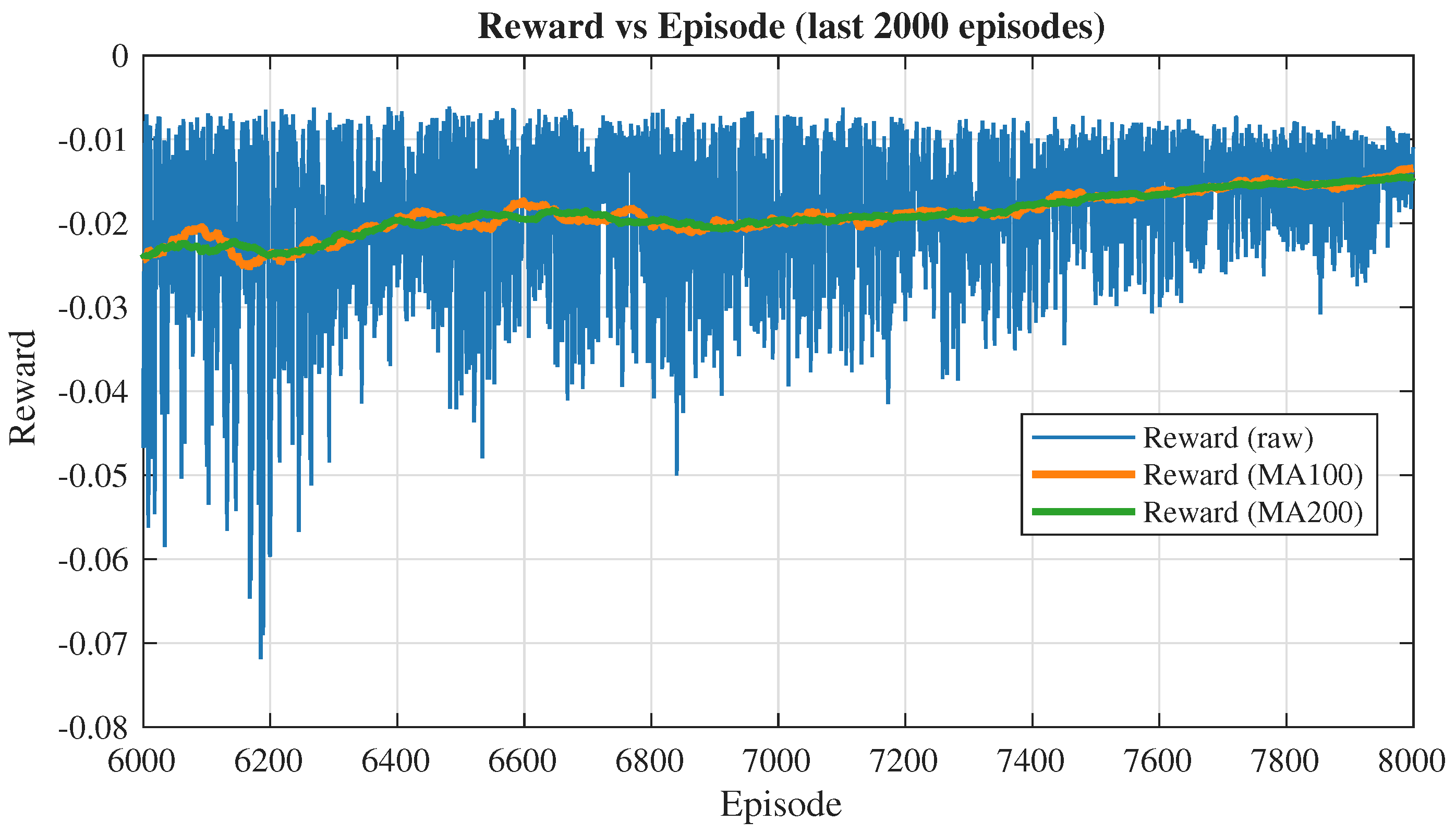
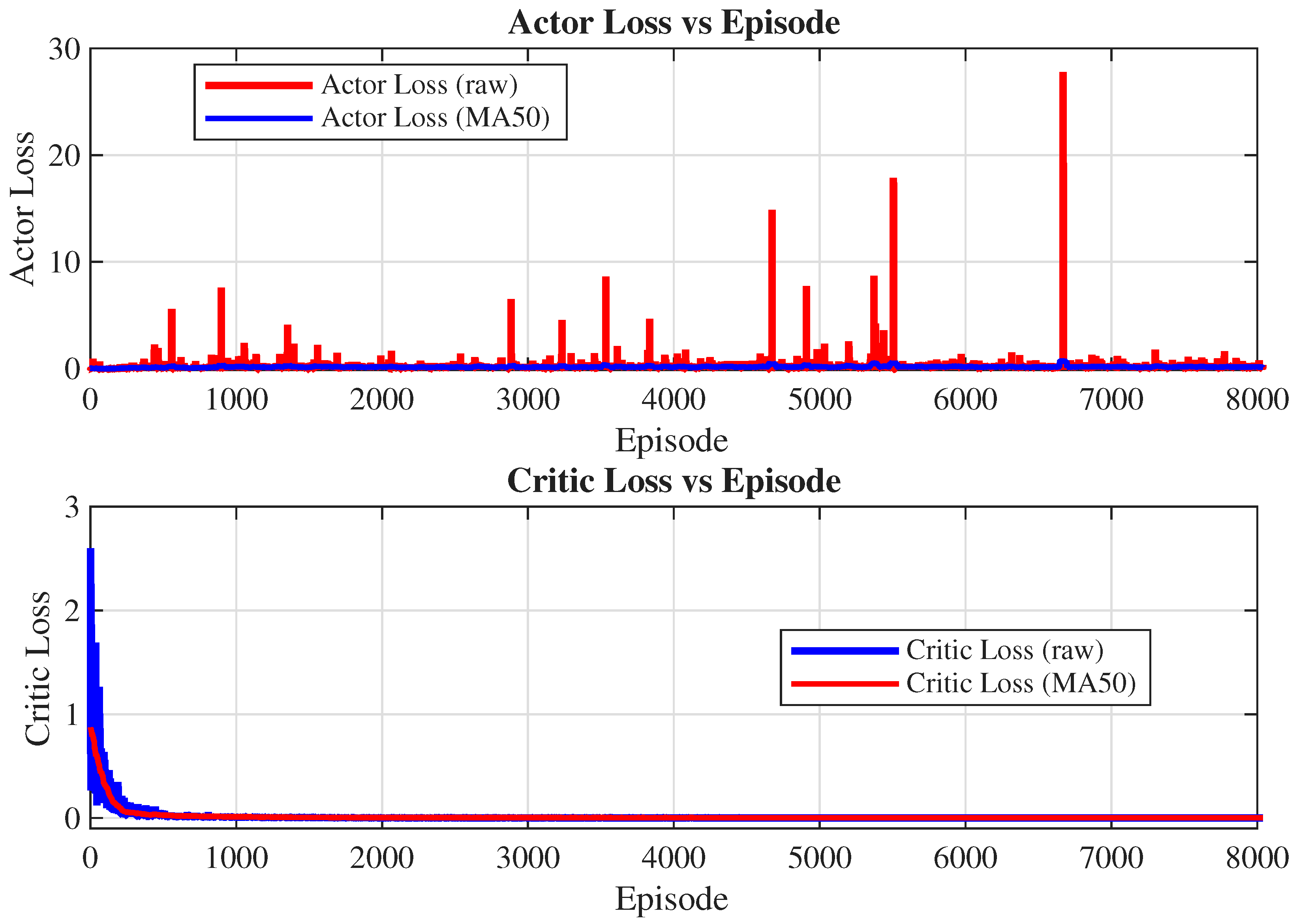
Machines 14 00672 g011
Figure 12. Actor and critic loss curves.
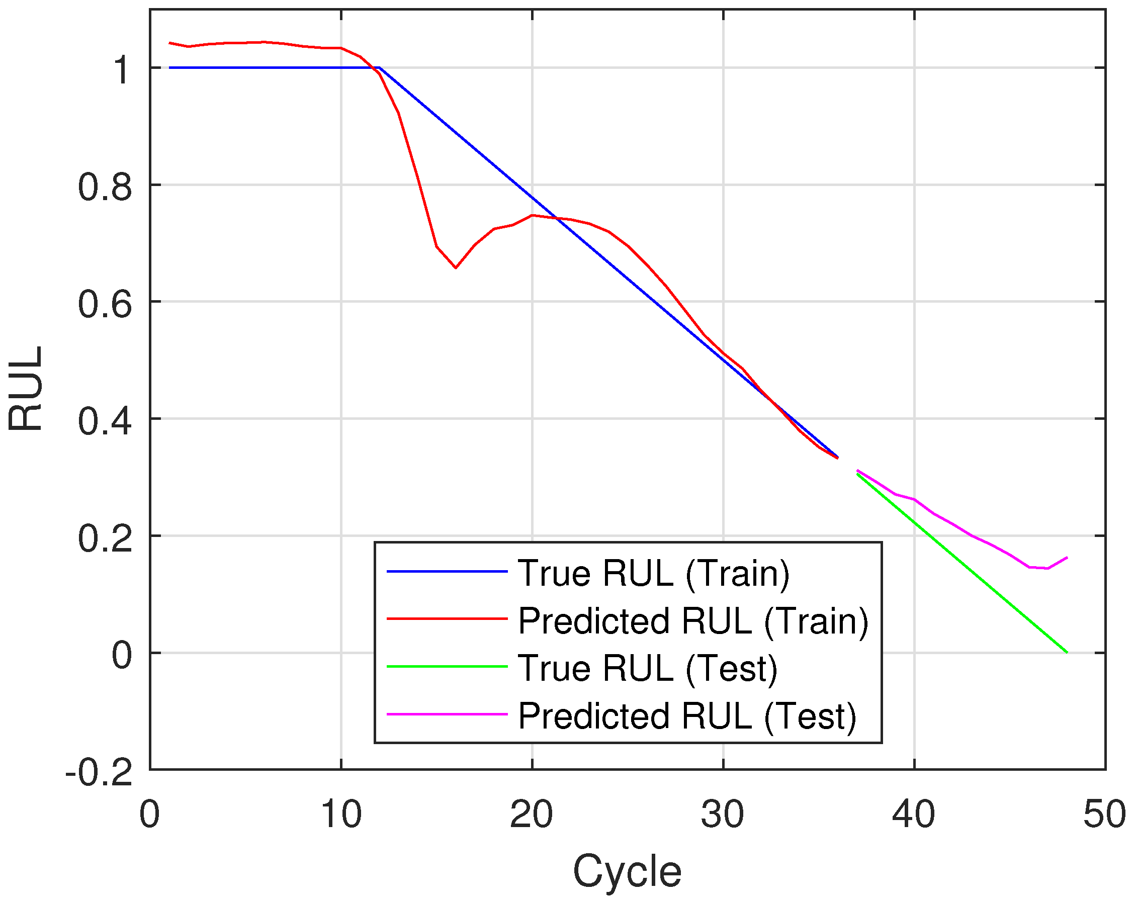
Machines 14 00672 g012
Figure 13. PPO training and testing predictions.
Machines 14 00672 g013
Figure 14. Naive linear regression training and testing predictions.
Machines 14 00672 g014
Figure 15. LSTM training and testing predictions.
Machines 14 00672 g015
Figure 16. MLP training and testing predictions.
Machines 14 00672 g016
Table 1. Core components of the DRL framework and their interpretation in the context of RUL estimation.
ComponentDescription
AgentThe agent interacts with the environment by observing its state and executing actions, receiving a reward in return. In RUL estimation, the agent learns to predict the RUL based on the degradation state of the machine, typically from extracted features.
ActionThe action is what the agent does in the environment based on its policy, and can be either discrete (a finite set of choices) or continuous (a value-attached choice). For RUL applications, the action represents the predicted RUL value, typically scaled between 100% and 0% health.
EnvironmentThe external system with which the agent interacts, defining the state space, action space, and the rules governing transitions and rewards. In RUL estimation, the environment is modelled using historical run-to-failure data, evolving as the component degrades and allowing the agent to learn degradation patterns through interaction.
RewardA scalar feedback signal provided by the environment after each action, indicating whether the action was favourable or unfavourable. The agent aims to maximize the cumulative reward over a sequence of actions. In RUL estimation, the reward is typically based on prediction error, with smaller errors yielding higher rewards.
ObservationsThe information the environment provides to the agent, serving as the input for action selection. In RUL settings, observations are typically extracted features from sensor signals (such as vibration data) that reflect the component’s current health condition.
PolicyThe strategy the agent follows to select actions from its observations, either a deterministic mapping or a probability distribution over actions. For RUL prediction, the policy learns to map health indicators to RUL estimates.
Table 3. Statistical time-domain features.
FeatureDefinition *
Mean x ¯ = 1 n k = 1 n | x k |
Maximum Value x ^ = max ( x )
Root Mean Square R M S = 1 n k = 1 n ( x k ) 2
Square Root Mean S R M = ( 1 n k = 1 n | x k | ) 2
Standard Deviation σ = 1 n k = 1 n ( x k x ¯ ) 2
Kurtosis k = 1 n k = 1 n ( x k x ¯ ) 4 σ 4
* n is the total number of the elements of vector X, whilst x k is the kth element.
Table 4. PPO network architecture.
ComponentActor NetworkCritic Network
Input Dimensions55
Hidden Layers1 layer with 32 neurons1 layer with 32 neurons
ActivationReLUReLU
Output DimensionsMean + STD (Gaussian Distribution)Single scalar value ( V ( s ) )
Output ActivationsSigmoid (mean), Softplus (STD)None
Table 5. PPO training parameters.
ParameterValue
Training episodes8000
Discount factor0.99
Lambda for GAE0.95
Clipping ratio0.2
Batch size32
Policy optimization algorithmAdam
Policy learning rate 5 × 10 4
Value optimization algorithmAdam
Value learning rate 1 × 10 3
Buffer size2000
Epochs10
Entropy Coefficient0.01
Table 6. LSTM network architecture.
ComponentDescription
Input DimensionsObservation sequence of size 5 × 30 (5 features over 30 time steps)
Recurrent Layer 1LSTM layer with 64 hidden units
Normalization 1Batch normalization (applied after LSTM-64)
ActivationReLU
Recurrent Layer 2LSTM layer with 32 hidden units
Normalization 2Batch normalization (applied after LSTM-32)
RegularizationDropout rate of 0.2
PoolingGlobal average pooling (temporal aggregation)
Output LayerFully connected layer with 1 neuron
Output ActivationLinear
OutputScalar prediction: estimated bearing RUL
Table 7. MLP network architecture for bearing RUL estimation.
ComponentDescription
Input Dimensions 5 × 30 dimensional observation/feature vector
Hidden Layer 1Fully connected (dense) layer with 64 neurons
Activation (Layer 1)ReLU
RegularizationDropout rate of 0.2 (applied after Layer 1)
Hidden Layer 2Fully connected (dense) layer with 32 neurons
NormalizationBatch normalization (applied after Layer 2)
Activation (Layer 2)ReLU
Output LayerFully connected layer with 1 neuron
Output ActivationLinear
OutputScalar prediction: estimated bearing RUL
Table 8. Train and test results for RUL estimation.
MethodTrain ResultsTest Results
ScoreMAERMSEMSEScoreMAERMSEMSE
PPO0.20020.06140.07960.00630.05120.05260.06940.0048
Linear Regression0.13860.04460.05400.00290.11720.09710.09930.0099
LSTM0.18940.04550.06940.00480.19850.11940.08190.0067
MLP0.11520.03490.04600.00210.58500.15750.09410.0089
Disclaimer/Publisher’s Note: The statements, opinions and data contained in all publications are solely those of the individual author(s) and contributor(s) and not of MDPI and/or the editor(s). MDPI and/or the editor(s) disclaim responsibility for any injury to people or property resulting from any ideas, methods, instructions or products referred to in the content.