Adaptive Optimal Speed Tracking Control of a PMSM Integrated with Linear Quadratic Integral Control for the Peak DC-Link Voltage Regulation of Quasi-Z-Source Inverters in All-Electric Aircraft

Abstract

This paper proposes an optimal tracking control framework for a permanent magnet synchronous motor (PMSM) drive integrated with a quasi-Z-source (QZS) inverter for all-electric aircraft applications. Two tracking control strategies are developed: (i) an online adaptive optimal control (OAC) method for tracking motor speed and (ii) a linear quadratic integral (LQI) controller for regulating the peak DC-link voltage (PDV) of the QZS. Due to the nonlinear characteristics, parameter uncertainties, and external disturbances inherent in PMSM systems, achieving accurate speed tracking and stable DC-link voltage (DCV) regulation using a PDV control strategy under varying power flow conditions remains a significant challenge. In this study, the PMSM model is represented as a nonlinear system with strict feedback. Augmented feedforward control signals are incorporated to restructure the conventional cascade control architecture into a novel optimal control framework. Based on this formulation, a saturated adaptive optimal control law is proposed, relying on a near-optimal solution to the Hamilton–Jacobi–Isaacs (HJI) equation. This solution is approximated using an online approximator combined with an integral reinforcement learning technique. Meanwhile, an LQI controller is employed to regulate the PDV and suppress voltage fluctuations in the QZS. Simulation results demonstrate that the proposed approach significantly improves speed tracking accuracy, DCV stability, and disturbance rejection capability while improving the overall performance and reliability of PMSM drive systems. The simulation results demonstrate that the proposed control strategies have strong potential for effective application in all-electric aircraft systems, meeting the requirements of high performance and energy efficiency.

1. Introduction

In recent years, the rapidly increasing demand for small-scale all-electric aircraft has imposed increasingly stringent requirements on motor control strategies and power electronic systems to enhance efficiency, reliability, safety, and overall system performance [1]. In this context, permanent magnet synchronous motors have been increasingly widely adopted due to their superior efficiency and high power density [1]. However, the application of these motors in harsh environments such as aerospace requires sophisticated control mechanisms to effectively address critical challenges, including torque oscillations and nonlinear tracking characteristics [2,3]. Specifically, the inherent characteristics of a PMSM, such as trapezoidal back electromotive force (EMF) waveforms, often induce torque ripple, thereby degrading the operational quality of the drive system. Therefore, it is necessary to develop and implement advanced control techniques to ensure smooth operation and to enhance the overall performance of PMSM drive systems [4].

Moreover, the gradual degradation of battery voltage over operating time has a significant impact on the speed regulation capability of PMSM drives. When the source voltage falls below the permissible threshold, the inverter may operate in the overmodulation region, leading to a substantial increase in current harmonics, which consequently reduces the motor’s lifetime and reliability [5]. Therefore, replacing conventional DC–DC converters with quasi-Z-source topologies in PMSM drive systems (PZI) for electric vehicle and all-electric aircraft applications is regarded as a crucial solution to improve voltage regulation capability, enhance system robustness, and strengthen operational reliability [6].

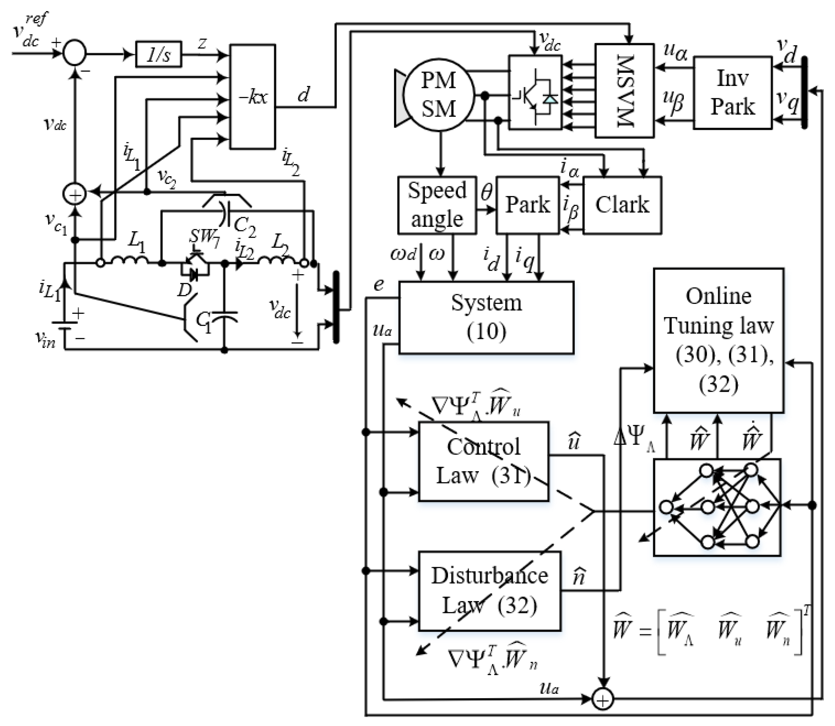
The motor speed control method for the PZI system in all-electric aircraft control applications still exhibits some limitations based on field-oriented control. Within the FOC framework, the control structure is organized in a cascade form with three proportional–integral (PI) controllers that are tightly coupled to ensure high-precision regulation of speed and current [7]. In this control system, the QZS converter is integrated to replace the conventional DC–DC converter and is connected upstream of the inverter, as illustrated in Figure 1. The QZS topology not only enables power recovery to the battery during deceleration or regenerative braking modes but also plays a critical role in stabilizing the system voltage [6]. The output voltage of the QZS, referred to as the DPV, is regulated and directly supplied to the inverter.

The DPV control method is designed in a cascade structure, where the inner loop regulates the inductor current and the outer loop controls the capacitor voltage [6]. Consequently, the overall PZI control framework in all-electric aircraft applications comprises a total of five PI controllers. However, the tuning of these PI controller parameters remains a significant challenge due to the presence of time-varying factors, such as motor speed, PDV, PMSM resistance parameters, load torque, system disturbances, and aerodynamic effects such as gusts [8]. Therefore, the design of effective controllers for PMSM drives as well as robust PDV regulation continues to be a complex problem and has attracted considerable attention in recent research.

Regarding PMSM speed control in recent years, numerous studies have proposed speed-tracking control strategies for PMSM drives, including optimization methods based on particle swarm optimization [9] and Fuzzy-PID controllers [10]. However, achieving accurate and stable speed responses remains a significant challenge under load conditions and external disturbances. To overcome the limitations of conventional control approaches and to meet the requirements of reliability, safety, and optimality, reinforcement learning (RL) has been considered a promising alternative approach [11]. With the advantages of RL theory and the use of approximation techniques to solve the HJB equation, the optimal value function and optimal control law can be determined. Nevertheless, most existing studies have not sufficiently addressed the effects of torque disturbances, control voltages in the dq-axis [6], or the degradation of the PDV [12].

Many related studies have addressed this issue. Farbood et al. [13] focuses on developing a Model Predictive Control (MPC) approach for nonlinear systems by employing a Takagi–Sugeno (T–S) fuzzy model combined with a Quadratic Programming (QP) optimization framework. However, the control performance of this method strongly depends on the number of fuzzy sets, which may increase the computational burden and affect the hardware execution speed. Furthermore, Palangari et al. [14] focuses on developing an optimal power control strategy for EV charging stations with Vehicle-to-Grid (V2G) capability using an Event-Triggered Model Predictive Control (ET-MPC) approach. Nevertheless, the issues of system stability and enhancement of the DC-link voltage quality supplied to the inverter under input voltage reduction during operation have not been addressed. In addition, Farbood et al. [15] develops a Data-Driven Model Predictive Control (DD-MPC) method combined with a Disturbance Observer (DOB) to improve tracking performance and disturbance rejection for linear systems. However, this study does not consider mathematical model uncertainties, disturbances such as wind gusts and battery voltage reduction, or model prediction errors. Therefore, to address the aforementioned limitations, a promising research direction proposed in recent years is the online adaptive optimal trajectory tracking control approach for the speed of PMSMs.

The main approach of this research direction is the approximation-based method when the mathematical model of the plant is not fully known, particularly for PMSM drives applied in all-electric aircraft under the effects of torque disturbances, voltage fluctuations, parameter uncertainties, and wind gusts. The proposed control strategy is developed using approximation techniques to obtain an approximate solution of the Hamilton–Jacobi–Isaacs (HJI) equation, which represents the derivative of the cost function ($\Lambda$). Based on this formulation and in conjunction with the two-player zero-sum (ZS) game theory [16], the optimal control and disturbance laws are simultaneously derived for the q-axis current and dq-axis voltages. In addition, the influence of the DC-link voltage on tracking performance is comprehensively investigated, and an LQI control scheme is integrated for PDV regulation, thus enhancing the overall stability and robustness of the system.

Within the framework of proposing a speed control method for PMSM drives, this paper exploits RL in conjunction with the approximation of the HJI equation to derive the optimal control law. The primary objective is to ensure that the PMSM speed accurately tracks its reference speed in the presence of disturbances while simultaneously satisfying the criterion of battery power optimization. This approach enables the control problem to be modeled as an optimal system with online adaptive capability, thereby enhancing the reliability and performance of PMSM drive systems under complex operating conditions.

The core idea of the proposed approach is to formulate the control problem as a two-player zero-sum game, where the first player represents the control law and the second player represents disturbances. Based on this formulation, the solution of the HJI equation is obtained in real time through an online learning mechanism grounded in the policy iteration principle [17]. The learning process enables the simultaneous derivation of the control law, the disturbance law, and a near-optimal value function, thereby significantly improving the speed response and maintaining the stability of the motor speed even under parameter variations and disturbances.

In addition to developing a speed-tracking controller for PMSM drives, many studies have also focused on improving power quality and stabilizing the input voltage supplied to inverters based on the QZS topology [18]. In particular, during operation, the battery voltage tends to degrade over time; if the DC-link voltage is not maintained at a stable level, the speed response of the PMSM will be significantly affected [19,20]. This issue may reduce system reliability, compromise operational safety, and increase motor thermal stress due to harmonic effects, thereby shortening the lifetime of the drive system [18]. Therefore, the regulation and stabilization of the DC-link voltage in QZS-based inverters are of critical importance.

In previous studies, Pham et al. [6] propose the DC-link voltage of the quasi-Z-source converter exhibits a square-wave characteristic; therefore, direct control of this variable is not feasible. Consequently, it is indirectly regulated through the combined voltages across capacitors $C_1$ and $C_2$, as illustrated in Figure 1. The total voltage across these two capacitors represents the peak DC-link voltage (PDV) in the QZS topology [6]. Owing to the nonlinear relationship between the modulation index d and the total voltage across the two capacitors of the QZS network, the application of conventional FF controllers often fails to guarantee satisfactory DC-link voltage regulation performance. As a consequence, the voltage supplied to the inverter does not achieve the desired accuracy, leading to degradation in the overall performance of the drive system, even when the motor speed controller has been optimally designed.

Therefore, in addition to proposing an online adaptive optimal control method for PMSM speed regulation, this paper also presents an LQI control method to enhance the regulation capability of the PDV supplied to the inverter in the PZI structure, as illustrated in Figure 1. The proposed approach improves the flexibility and accuracy of voltage regulation, thereby contributing to enhanced stability and performance of the drive system under nonlinear operating conditions and parameter variations.

Despite these advances, several important limitations still remain in existing PMSM drive control strategies for all-electric aircraft applications. First, most existing methods mainly focus on PMSM speed regulation without considering the coordinated control between motor dynamics and DC-link voltage stabilization in quasi-Z-source inverter systems. Second, conventional PI/FOC-based structures require multiple cascaded controllers, whose tuning becomes difficult under parameter uncertainties, load disturbances, and battery voltage degradation. Third, although reinforcement learning and adaptive optimal control techniques have shown promising results, their applications to integrated PMSM–QZSI systems with simultaneous disturbance rejection and PDV regulation remain insufficiently investigated. Therefore, the development of a robust integrated control framework capable of handling nonlinear uncertainties, external disturbances, and DC-link voltage regulation simultaneously is still an open research challenge. The overall architecture of the proposed online adaptive optimal PMSM speed control integrated with the PZI topology is shown in Figure 1.

The main contributions of this paper are summarized as follows:

• An optimal tracking control framework for a PMSM drive integrated with a quasi-Z-source (QZS) inverter is proposed for all-electric aircraft applications, aiming to enhance motor speed tracking performance and DC-link voltage stability under varying operating conditions.
• A novel online adaptive optimal control (OAC) strategy is developed for PMSM speed regulation. The PMSM dynamics are formulated as a nonlinear strict-feedback system, while augmented feedforward control signals are introduced to reconstruct the conventional cascade control structure into an optimal control framework.
• A saturated adaptive optimal control law is designed based on a near-optimal solution of the Hamilton–Jacobi–Isaacs (HJI) equation. The unknown optimal solution is approximated online using an adaptive approximator combined with an integral reinforcement learning technique, eliminating the requirement for an accurate mathematical model.
• An LQI-based peak DC-link voltage (PDV) control strategy is proposed for the QZS network to regulate the DC-link voltage and suppress voltage fluctuations caused by varying power flow conditions.
• The proposed control framework simultaneously considers parameter uncertainties and external disturbances, including torque disturbances and voltage variations, thereby improving the robustness and disturbance rejection capability of the PMSM drive system.
• Simulation results verify that the proposed method achieves superior speed tracking accuracy, enhanced DC-link voltage stability, and improved overall system reliability compared with conventional control approaches, demonstrating strong potential for application in all-electric aircraft systems.

This paper is organized as follows: Section 2 presents the mathematical models of the PMSM and the QZS inverter. Section 3 develops the proposed OAC method for motor speed control. Section 4 presents the QZS model and designs the PDV controller in the QZS. Section 5 presents simulation results used to evaluate the effectiveness of the proposed control strategies for the PZI system in all-electric aircraft applications. Finally, the conclusions of this paper are summarized in Section 6.

2. The PMSM Model and Design Control Laws

Figure 1 depicts the overall system architecture, highlighting the dual-controller framework designed for PMSM speed tracking and DVP regulation. In practical applications, the derivation of an accurate model for this topology is challenging because of parametric uncertainties, such as varying motor speeds, load torque disturbances, and unstable DC input voltages. Therefore, this section formulates the mathematical model of the PMSM to construct an augmented feedforward control strategy.

Furthermore, the governing equations of the QZS system are presented in (33), serving as the basis for developing the DVP controller via the frequency-response method.

2.1. The PMSM Model

The dynamic behavior of the PMSM is described in the synchronous $dq$-axis reference frame by the state-space representation [21]:

$$\left\{\begin{array}{c}\dot{\omega }=-{\displaystyle \frac{B}{J}}\omega -{\displaystyle \frac{T_L}{J}}+{\displaystyle \frac{1.5n_p{\psi }_f}{J}}{i}_q+{\displaystyle \frac{n_{\tau }}{J}}\hfill \\ {\dot{i}}_d=-{\displaystyle \frac{R_s}{L_d}}{i}_d+n_p\omega i_q+{\displaystyle \frac{1}{L_d}}{v}_d+n_d\hfill \\ {\dot{i}}_q=-n_p\omega i_d-{\displaystyle \frac{R_s}{L_d}}{i}_q-n_p{\displaystyle \frac{{\psi }_f}{L_q}}\omega +{\displaystyle \frac{1}{L_q}}{v}_q+n_q\hfill \end{array}\right.$$

(1)

In this framework, $\omega$ denotes the angular velocity of the PMSM, while the stator voltage and current components decomposed in the synchronous $dq$-frame are represented by $(v_d,v_q)$ and $(i_d,i_q)$, respectively. To ensure stable operation, the voltage magnitudes are constrained such that $|v_d|<\lambda$ and $|v_q|<\lambda$, where $\lambda$ ($0<\lambda <1$) signifies the normalized voltage saturation limit. Regarding the machine’s electrical characteristics, $R_s$ stands for the stator resistance, ${\psi }_f$ is the constant flux linkage of the permanent magnets, and $L_d,L_q$ are the $dq$-axis inductances (assuming $L_d=L_q$ for a non-salient pole machine). The mechanical dynamics are governed by the viscous friction coefficient B, the moment of inertia J, the external load torque $T_L$, and the number of pole pairs $n_p$.

2.2. Design Control Laws for the Speed of PMSM

To transform the optimal tracking problem (1) into an affine form, a feedforward compensator is integrated into the PMSM speed control system [7]. For PMSM control applications, a feedforward control mechanism is introduced to convert the optimal tracking problem into a control-affine system representation. Based on this transformation, the system is rewritten in the error coordinate system, including the PMSM speed tracking error and the $dq$-axis current error states.

The PMSM speed tracking error and the corresponding virtual control inputs associated with the $dq$-axis currents are defined as follows.

From (1), the PMSM speed tracking error is defined as the difference between the measured speed and its reference signal. The $dq$-axis currents are considered virtual control inputs to the $dq$-axis voltage control loop [22], as illustrated in Figure 1. Consequently, the PMSM speed tracking error and the tracking errors of the $dq$-axis currents are defined as

$$\begin{array}{c}\left\{\begin{array}{c}{e}_{\omega }=\omega -{\omega }_d\hfill \\ e_{i_d}=i_d-i_d^d\hfill \\ e_{i_q}=i_q-i_q^d\hfill \end{array}\right.\end{array}$$

(2)

where ${\omega }_d$ represents the desired (reference) speed of the PMSM; $i_d^d$ and $i_q^d$ represent the desired reference currents in the $dq$-axis, respectively. The error variables $e_{\omega }$, $e_{i_d}$ and $e_{i_q}$ represent the speed and $dq$-axis current tracking errors, defined as the differences between the actual PMSM states and their corresponding reference values. Based on the PMSM mathematical model in (1), the speed tracking error of the PMSM speed can be reformulated as follows:

$${\dot{e}}_{\omega }=-{\dot{\omega }}_d-{\displaystyle \frac{B}{J}}\omega -{\displaystyle \frac{T_L}{J}}+{\displaystyle \frac{1.5n_p{\psi }_f}{J}}{e}_{i_q}+{\displaystyle \frac{1.5n_p{\psi }_f}{J}}{i}_q^d+{\displaystyle \frac{n_{\tau }}{J}}$$

(3)

As depicted in Figure 1, the reference currents $i_d^d$ and $i_q^d$ are regarded as virtual control variables corresponding to the $dq$-axis voltage control loop. Specifically, the virtual inputs include the adaptive optimal feedback components $i_d^{*}$ and $i_q^{*}$ as well as the feedforward augmentation terms $i_d^a$ and $i_q^a$ defined in the $dq$-axis reference frame [21]. Accordingly, the virtual control inputs are expressed as

$$\begin{array}{c}\left\{\begin{array}{c}{i}_d^d=i_d^{*}+i_d^a\hfill \\ i_q^d=i_q^{*}+i_q^a\hfill \end{array}\right.\end{array}$$

(4)

The enhanced feedforward control component of the d-axis current is set to zero, whereas the q-axis component is designed as follows:

$$\left\{\begin{array}{c}{i}_d^a=0\hfill \\ i_q^a={\displaystyle \frac{J}{1.5n_p{\psi }_f}}\left({\dot{\omega }}_d-{\gamma }_{{\omega }_I}{\int }_0^t{e}_{\omega }\left(\tau \right)d\tau -{\gamma }_{{\omega }_P}{e}_{\omega }\right)-{\gamma }_i{e}_{i_q}\hfill \end{array}\right.$$

(5)

where ${\gamma }_{{\omega }_I},{\gamma }_{{\omega }_P}\ge 0$ and $0\le {\gamma }_i\le 1$ denote the design parameters. Substituting Equation (5) and Equation (4) into Equation (3) yields the reformulated PMSM speed tracking error dynamics as follows:

$$\begin{array}{cc}\hfill {\dot{e}}_{\omega }& =-{\dot{\omega }}_d-{\displaystyle \frac{B}{J}}\omega -{\displaystyle \frac{T_L}{J}}+{\displaystyle \frac{1.5n_p{\psi }_f}{J}}{e}_{i_q}+{\displaystyle \frac{1.5n_p{\psi }_f}{J}}{i}_q^{*}\hfill \\ \hfill & +{\displaystyle \frac{1.5n_p{\psi }_f}{J}}\left[{\displaystyle \frac{J}{1.5n_p{\psi }_f}}\right({\dot{\omega }}_d-{\gamma }_{{\omega }_I}{\int }_0^t{e}_{\omega }\left(\tau \right)d\tau \hfill \\ \hfill & -{\gamma }_{{\omega }_P}{e}_{\omega })-{\gamma }_i{e}_{i_q}]+{\displaystyle \frac{n_{\tau }}{J}}\hfill \\ \hfill \Rightarrow {\dot{e}}_{\omega }& =-{\displaystyle \frac{B}{J}}\omega -{\displaystyle \frac{T_L}{J}}+{\displaystyle \frac{1.5n_p{\psi }_f}{J}}(1-{\gamma }_i)e_{i_q}-{\gamma }_{{\omega }_P}{e}_{\omega }\hfill \\ \hfill & -{\gamma }_{{\omega }_I}{\int }_0^t{e}_{\omega }\left(\tau \right)d\tau +{\displaystyle \frac{1.5n_p{\psi }_f}{J}}{i}_q^{*}+{\displaystyle \frac{n_{\tau }}{J}}\hfill \end{array}$$

(6)

The $dq$-axis current tracking errors, together with the corresponding virtual control inputs associated with the $dq$-axis voltages, are defined as follows:

The $dq$-axis voltage control inputs ($v_d$ and $v_q$) in (1) are composed of two components: the overall control law includes the adaptive optimal feedback signals ($v_d^{*}$ and $v_q^{*}$) augmented by feedforward compensation components ($v_d^a$ and $v_q^a$) [7,23,24]. As shown in Figure 1, these control signals are represented by the following mathematical expressions:

$$\begin{array}{c}\left\{\begin{array}{c}{v}_d=v_d^{*}+v_d^a\hfill \\ v_q=v_q^{*}+v_q^a\hfill \end{array}\right.\end{array}$$

(7)

where the feedforward ($v_d^a$ and $v_q^a$) augmentation terms are formulated as

$$\begin{array}{c}\left\{\begin{array}{c}{v}_d^a=L_d{\dot{i}}_d^d-{\gamma }_{d_I}{\int }_0^t{e}_{i_d}\left(\tau \right)d\tau -{\gamma }_{d_P}{e}_{i_d}\hfill \\ v_q^a=L_q{\dot{i}}_q^d-{\displaystyle \frac{1.5n_p{\psi }_f}{J}}(1-{\gamma }_i)e_{\omega }\hfill \\ -{\gamma }_{q_I}{\int }_0^t{e}_{i_q}\left(\tau \right)d\tau -{\gamma }_{q_I}{e}_{i_q}\hfill \end{array}\right.\end{array}$$

(8)

where ${\gamma }_{d_I}>0$, ${\gamma }_{d_P}>0$, ${\gamma }_{q_I}>0$ and ${\gamma }_{q_P}>0$ denote the design parameters. Substituting (8) into (7) and substituting (7) into (1), and using the definitions given in (2), yields the reformulated $dq$-axis current tracking error dynamics as follows:

$$\begin{array}{c}\left\{\begin{array}{c}{\dot{e}}_{i_d}=-{\displaystyle \frac{R_s}{L_d}}{i}_d+n_p\omega i_q\hfill \\ -{\displaystyle \frac{1}{L_d}}\left({\gamma }_{d_i}{\int }_0^t{e}_{i_d}\left(\tau \right)d\tau +{\gamma }_{d_P}{e}_{i_d}\right)+{\displaystyle \frac{1}{L_d}}{v}_d^{*}+n_d\hfill \\ {\dot{e}}_{i_q}=-n_p\omega i_d-{\displaystyle \frac{R_s}{L_q}}{i}_q-n_p{\displaystyle \frac{{\psi }_f}{L_q}}\omega -{\displaystyle \frac{1.5n_p{\psi }_f}{J}}(1-{\gamma }_i)e_{\omega }\hfill \\ -{\displaystyle \frac{1}{L_q}}\left({\gamma }_{q_I}{\int }_0^t{e}_{i_q}\left(\tau \right)d\tau +{\gamma }_{q_p}{e}_{i_q}\right)+{\displaystyle \frac{1}{L_q}}{v}_q^{*}+n_q\hfill \end{array}\right.\end{array}$$

(9)

By combining (3) with (9), the system equations can be reformulated as follows:

$$\begin{array}{c}\left\{\begin{array}{c}{\dot{e}}_{\omega }=-{\displaystyle \frac{B}{J}}\omega -{\displaystyle \frac{T_L}{J}}-{\gamma }_{{\omega }_I}{\int }_0^t{e}_{\omega }\left(\tau \right)d\tau -{\gamma }_{{\omega }_P}{e}_{\omega }+{\displaystyle \frac{1.5n_p{\psi }_f}{J}}{i}_q^{*}+{\displaystyle \frac{1}{J}}{n}_{\tau }\hfill \\ {\dot{e}}_{i_d}=-{\displaystyle \frac{R_s}{L_d}}{i}_d+n_p\omega i_q-{\displaystyle \frac{\mathbf{1}}{{\mathit{L}}_{\mathit{d}}}}\mathbf{·}\left({\gamma }_{d_i}{\int }_0^t{e}_{i_d}\left(\tau \right)d\tau +{\gamma }_{d_P}{e}_{i_d}\right)+{\displaystyle \frac{\mathbf{1}}{{\mathit{L}}_{\mathit{d}}}}\mathbf{·}{\mathit{v}}_{\mathit{d}}^{\mathbf{*}}+n_d\hfill \\ {\dot{e}}_{i_q}=-n_p\omega i_d-{\displaystyle \frac{R_s}{L_d}}{i}_q-n_p{\displaystyle \frac{{\psi }_f}{L_q}}\omega -{\displaystyle \frac{1}{L_q}}\left({\gamma }_{q_I}{\int }_0^t{e}_{i_q}\left(\tau \right)d\tau +{\gamma }_{q_p}{e}_{i_q}\right)+{\displaystyle \frac{\mathbf{1}}{{\mathit{L}}_{\mathit{q}}}}\mathbf{·}{\mathit{v}}_{\mathit{q}}^{\mathbf{*}}+n_q\hfill \end{array}\right.\end{array}$$

(10)

Theorem 1.

The strict-feedback representation of the PZI scheme is transformed into control system (10) by incorporating (4), (6) and (7), where the feedforward augmentation terms associated with the q-axis current are defined in (5), while the augmented feedforward control inputs for the $dq$-axis voltages are formulated as in (8). The adaptive optimal control input vector, represented by $u^{*}$, is given by $u^{*}={\left[\begin{array}{ccc}{i}_q^{*}& v_d^{*}& v_q^{*}\end{array}\right]}^T$, and the control law $u^{*}$ is assumed to stabilize the closed-loop PMSM speed control system, as shown in Figure 1. The variable n denotes the disturbance signals. Accordingly, the system dynamics can be summarized as follows:

$$\dot{e}=f\left(e\right)+g\left(e\right)u^{*}+k\left(e\right)n$$

(11)

where

$$\begin{array}{cc}\hfill e& ={\left[\begin{array}{ccc}{e}_{\omega }& e_{id}& e_{iq}\end{array}\right]}^T;n={\left[\begin{array}{ccc}{n}_{\tau }& n_d& n_q\end{array}\right]}^T;f={\left[\begin{array}{ccc}{f}_1& f_2& f_3\end{array}\right]}^T;g={\left[\begin{array}{ccc}{g}_1& g_2& g_3\end{array}\right]}^T\hfill \\ \hfill k& =\left[\begin{array}{ccc}{\displaystyle \frac{1}{J}}& 0& 0\\ 0& 1& 0\\ 0& 0& 1\end{array}\right];f_1=-{\displaystyle \frac{B}{J}}\omega -{\displaystyle \frac{T_L}{J}}-{\gamma }_{{\omega }_I}{\int }_0^t{e}_{\omega }\left(\tau \right)d\tau -{\gamma }_{{\omega }_P}{e}_{\omega }\hfill \\ \hfill f_2& =-{\displaystyle \frac{R_s}{L_d}}{i}_d+n_p\omega i_q-{\displaystyle \frac{1}{L_d}}\left({\gamma }_{d_i}{\int }_0^t{e}_{i_d}\left(\tau \right)d\tau +{\gamma }_{d_P}{e}_{i_d}\right)\hfill \\ \hfill f_3& =-n_p\omega i_d-{\displaystyle \frac{R_s}{L_q}}{i}_q-{\displaystyle \frac{n_p{\psi }_f}{L_q}}\omega -{\displaystyle \frac{1}{L_q}}\left({\gamma }_{qI}{\int }_0^t{e}_{i_q}\left(\tau \right)d\tau +{\gamma }_{qP}{e}_{i_q}\right)\hfill \\ \hfill g_1& ={\displaystyle \frac{1.5n_p{\psi }_f}{J}};g_2={\displaystyle \frac{1}{L_d}};g_3={\displaystyle \frac{1}{L_q}}\hfill \end{array}$$

where $f_1$ is considered to be an unknown nonlinear function. According to the aforementioned theorem, the online adaptive optimal tracking control problem associated with the strict-feedback system expressed in (1) can be converted into an equivalent optimal tracking control problem for the affine system represented in (11). The affine system is required to satisfy boundedness conditions, and the corresponding Assumption is stated as follows:

• Boundedness:
  Owing to the inherent physical properties of the PZI system, it is assumed that the following boundedness conditions hold: $\left|\right|J\left|\right|\le J_{max}$, $\left|\right|g_i\left|\right|\le \left|\right|g_{i_{max}}\left|\right|$, $\left|\right|f_i\left|\right|\le \left|\right|f_{i_{max}}\left|\right|$, i = 1 to 3, where $J_{max}$, $g_{i_{max}}$, and $f_{i_{max}}$ denote unknown positive constants. The term J represents the performance index, and $J_{max}$ denotes its maximum bound.
• Assumption:
  The PMSM reference speed ${\omega }_d$ is assumed to be bounded and sufficiently smooth [21,25]. In the presence of unknown system dynamics f, the adaptive optimal tracking control problem defined in (1) can be reformulated as an adaptive optimal tracking control problem for the affine system in (11), yielding the adaptive optimal control input $u^{*}$ and the disturbance signal n. The validity of this transformation has been demonstrated in [7].

Proof. 

For the considered system (1), the Lyapunov function is chosen as follows:

$$\begin{array}{ccc}\hfill V_1& =& {\displaystyle \frac{1}{2}}{e}_{\omega }^T{e}_{\omega }+{\displaystyle \frac{1}{2}}{e}_{i_d}^T{e}_{i_d}+{\displaystyle \frac{1}{2}}{e}_{i_q}^T{e}_{i_q}\hfill \end{array}$$

(12)

The time derivative of the Lyapunov function $V_1$ is given by

$$\begin{array}{cc}\hfill {\dot{V}}_1& =e_{\omega }^T{\dot{e}}_{\omega }+e_{i_d}^T{\dot{e}}_{i_d}+e_{i_q}^T{\dot{e}}_{i_q}+e_{v_c}^T{\dot{e}}_{v_c}+e_{i_L}^T{\dot{e}}_{i_L}\hfill \\ \hfill & =e_{\omega }^T\left[-{\displaystyle \frac{B}{J}}\omega -{\displaystyle \frac{T_L}{J}}-{\gamma }_{{\omega }_P}{e}_{\omega }-{\gamma }_{{\omega }_I}{\int }_0^t{e}_{\omega }\left(\tau \right)d\tau \right]\hfill \\ \hfill & +e_{\omega }^T{\displaystyle \frac{1.5n_p{\psi }_f}{J}}(1-{\gamma }_i)e_{i_q}\hfill \\ \hfill & +e_{i_d}^T[-{\displaystyle \frac{R_s}{L_d}}{i}_d+n_p\omega i_q+{\displaystyle \frac{1}{L_d}}{v}_d^{*}+n_d\hfill \\ \hfill & -{\displaystyle \frac{1}{L_d}}\left({\gamma }_{d_i}{\int }_0^t{e}_{i_d}\left(\tau \right)d\tau +{\gamma }_{d_P}{e}_{i_d}\right)]\hfill \\ \hfill & +e_{i_q}^T[-n_p\omega i_d-{\displaystyle \frac{R_s}{L_q}}{i}_q-{\displaystyle \frac{n_p{\psi }_f}{L_q}}\omega \hfill \\ \hfill & -{\displaystyle \frac{1}{L_q}}\left({\gamma }_{q_I}{\int }_0^t{e}_{i_q}\left(\tau \right)d\tau +{\gamma }_{q_p}{e}_{i_q}\right)\hfill \\ \hfill & +{\displaystyle \frac{1}{L_q}}{v}_q^{*}+n_q]\hfill \\ \hfill & -e_{i_q}^T{\displaystyle \frac{1.5n_p{\psi }_f}{J}}(1-{\gamma }_i)e_{\omega }\hfill \end{array}$$

(13)

Noting that scalars satisfy $e_{\omega }^T=e_{\omega }$ and $e_{i_q}^T=e_{i_q}$, the cross-coupling term can be expressed as

$$e_{\omega }^T{\displaystyle \frac{1.5n_p{\psi }_f}{J}}(1-{\gamma }_i)e_{i_q}=e_{i_q}^T{\displaystyle \frac{1.5n_p{\psi }_f}{J}}(1-{\gamma }_i)e_{\omega }$$

Therefore, (13) can be reformulated as follows:

$${\dot{V}}_1=e^T(f+g{u}^{*}+kn)=e^T\dot{e}$$

(14)

The derivative of the Lyapunov candidate function with respect to time is expressed as ${\dot{V}}_2$, which is computed along the trajectories of the strict-feedback system in (11).

$${\dot{V}}_2=e^T\dot{e}$$

(15)

According to Lyapunov stability theory, the strict-feedback system in (11) is stable under the control input $u^{*}$ if ${\dot{V}}_2$ is negative definite. Combining (14) and (15) yields ${\dot{V}}_1={\dot{V}}_2$. Consequently, ${\dot{V}}_1<0$, which guarantees that the PMSM speed tracking error in (10) is uniformly ultimately bounded (UUB) [7]. Therefore, the PMSM speed control problem described in (1) is equivalently converted into the adaptive optimal tracking control formulation given in (11). The proof is thus completed. □

3. Proposed Online Adaptive Optimal Tracking Control Strategy for PMSM Speed

It is known that the PMSM speed control input consists of two components: the enhanced feedforward term and the optimal term, as indicated in (4) and (7). The enhanced feedforward component has been proposed in (5) and (8), whereas the optimal component is addressed in this section. This optimal term is developed based on zero-sum differential game theory between two players: the optimal control input u and the disturbance signal n. The control player aims to minimize the value function, while the disturbance player seeks to maximize the value function in (21). The control structure for PMSM speed regulation is illustrated in Figure 1.

3.1. Theory of the Online Adaptive Optimal Tracking Control Strategy

In practical control systems, especially nonlinear systems such as PMSM speed regulation, the system dynamics f are typically uncertain or incompletely known owing to voltage disturbances, load variations, and wind gusts in all-electric aircraft applications. However, the proposed control framework is capable of updating the dynamics model f online; therefore, explicit identification of f is not required. The control laws for the q-axis current and the $dq$-axis voltages are collectively denoted by the control input u, and the disturbance law n is described in detail in this section. The control law of this system and the disturbance law are formulated as two competing agents in the RL framework, as illustrated in Figure 1 [24,26,27].

Using (11), the system dynamics can be expressed in the following form:

$$\dot{e}=f\left(e\right)+g\left(e\right)u+k\left(e\right)n$$

(16)

where the state vector, control input vector, and disturbance vector are defined as follows:

$$\begin{array}{cc}\hfill e& ={\left[\begin{array}{ccc}{e}_{\omega }& e_{id}& e_{iq}\end{array}\right]}^T\in {\mathbb{R}}^{3\times 1}\hfill \\ \hfill u& ={\left[\begin{array}{ccc}{i}_q& v_d& v_q\end{array}\right]}^T\in {\mathbb{R}}^{3\times 1}\hfill \\ \hfill n& ={\left[\begin{array}{ccc}{n}_{\tau }& n_d& n_q\end{array}\right]}^T\in {\mathbb{R}}^{3\times 1}\hfill \end{array}$$

The vector fields $f\left(e\right),g\left(e\right),k\left(e\right)\in {\mathbb{R}}^{3\times 1}$ correspond to the system dynamics in (11). The function $f\left(e\right)$ is assumed to be locally Lipschitz with $f\left(0\right)=0$, indicating that $e=0$ represents the equilibrium point of the transformed system in (11).

Following the design approach in [26], the performance index is defined as

$$J(e,u,n)={\int }_0^{\infty }\Gamma (e,u,n)dt$$

(17)

where $\Gamma (e,u,n)$ denotes the instantaneous cost (or utility) function, defined as follows:

$$\Gamma (e,u,n)=Q\left(e\right)+u^{T}Ru-{\gamma }^2{\parallel n\parallel }^2$$

In this formulation, $Q\left(e\right)$ denotes a positive definite function, and R is a symmetric positive definite matrix (i.e., $R=R^T>0$). The parameter $\gamma$ is a design factor satisfying $0\le {\gamma }^{*}\le \gamma$, where ${\gamma }^{*}$ is the minimum attenuation level required to stabilize the system.

Following [26], the value function $\Lambda (e,u,n)$ for system (11) is commonly referred to as the critic in the RL framework, and it is also defined as

$$\Lambda (e,u,n)={\int }_t^{\infty }\Gamma (e,u,n)d\tau$$

(18)

The function $\Lambda (e,u,n)$ is finite and satisfies $\Lambda \left(0\right)=0$.

By differentiating both sides of (18), the Bellman equation is given by

$$\begin{array}{c}\Gamma (e,u,n)+{\displaystyle \frac{\partial {\Lambda }^T\left(e\right)}{\partial e}}\dot{e}=0\\ ⟺\Gamma (e,u,n)+\mathsf{\nabla }{\Lambda }^T\left(e\right)(f\left(e\right)+g\left(e\right)u+k\left(e\right)n)=0\end{array}$$

(19)

Differential Equation (19) cannot be solved analytically; therefore, an approximation method must be employed to obtain the solution $\Lambda \left(e\right)$ of this equation. According to control theory [24], the Hamiltonian function is defined as

$$H(e,u,n,\mathsf{\nabla }\Lambda \left(e\right))=\Gamma (e,u,n)+\mathsf{\nabla }\Lambda {\left(e\right)}^{\top }\left(f\left(e\right)+g\left(e\right)u+k\left(e\right)n\right)$$

(20)

Within the framework of a two-player zero-sum game [24], the optimal value function is proposed as follows:

$$\begin{array}{cc}{\Lambda }^{*}\left(e\left(0\right)\right)=\underset{u}{\min }& \underset{n}{\max }J(e\left(0\right),u,n)\end{array}$$

(21)

Based on system (11), the control input u is treated as the minimizing player of the performance index $\Lambda (e,u,n)$, whereas the disturbance n is treated as the maximizing player. The existence of a saddle-point equilibrium [24] in this game guarantees the uniqueness of the solution to Equation (19), and this equation will be solved to determine the optimal solution ${\Lambda }^{*}\left(e\left(0\right)\right)$.

$$r(e,u^{*},n^{*})+\mathsf{\nabla }{\Lambda }^{oT}\left(e\right)(f+g{u}^{*}+k{n}^{*})=0$$

(22)

With the stationary condition of (27), ${\displaystyle \frac{\partial H(e,u,n,\mathsf{\nabla }\Lambda (e\left)\right)}{\partial u}}=0$ and ${\displaystyle \frac{\partial H(e,u,n,\mathsf{\nabla }\Lambda (e\left)\right)}{\partial n}}=0$, the saturated adaptive optimal control policy $u^{*}$ and the worst-case disturbance policy $n^{*}$ are derived as follows:

$$u^{*}=\arg \underset{u}{\min }H(e,u,n^{*},\mathsf{\nabla }{\Lambda }^{*}\left(e\right))=-{\displaystyle \frac{1}{2}}{R}^{-1}g{\left(e\right)}^T\mathsf{\nabla }{\Lambda }^{*}\left(e\right)$$

(23)

$$n^{*}=\arg \underset{n}{\max }H(e,u^{*},n,\mathsf{\nabla }{\Lambda }^{*}\left(e\right))={\displaystyle \frac{1}{2{\gamma }^2}}{k}^T\mathsf{\nabla }{\Lambda }^{*}\left(e\right)$$

(24)

3.2. Control and Disturbance Law Design for Online Adaptive Optimal Tracking Based on an Approximate Solution to the HJI Equation

Due to the analytical intractability of the HJI equation, reinforcement learning (RL) is adopted to obtain an online approximate solution and the corresponding optimal policies. The proposed framework employs an actor–critic structure with two actors and one critic. Two actors generate the optimal control law u and the disturbance law n, while the critic approximates the performance index $\Lambda \left(e\right)$. The value function $\Lambda \left(e\right)$ is approximated by the expression given in (25).

$$\Lambda \left(e\right)=W_{\Lambda }^T{\mathsf{\Psi }}_{\Lambda }\left(e\right)+ϵ\left(e\right)$$

(25)

where ${\mathsf{\Psi }}_{\Lambda }\left(e\right)$ denotes the activation function of the neural network, $ϵ\left(e\right)$ represents the approximation error of the cost value function, and $W_{\Lambda }$ denotes the ideal critic weight vector. The estimated weight vector is denoted by ${\widehat{W}}_{\Lambda }$, and the current critic approximation $\widehat{\Lambda }\left(e\right)$ is defined as follows:

$$\widehat{\Lambda }\left(e\right)={\widehat{W}}_{\Lambda }^T{\mathsf{\Psi }}_{\Lambda }\left(e\right)$$

(26)

Substituting (26) into (22), the approximated HJI equation can be rewritten as follows:

$$\begin{array}{cc}\hfill \widehat{H}(e,u,n,\mathsf{\nabla }\Lambda \left(e\right))& ={\widehat{W}}_{\Lambda }^{\top }\mathsf{\nabla }{\mathsf{\Psi }}_{\Lambda }\left(f\left(e\right)+g\left(e\right)\widehat{u}+k\left(e\right)\widehat{n}\right)+Q\left(e\right)+{\widehat{u}}^{\top }R\widehat{u}-{\gamma }^2{\parallel n\parallel }^2={ϵ}_1\hfill \end{array}$$

(27)

Here, ${ϵ}_1$ represents the approximation error for the HJI equation. Consequently, the adaptive optimal control law $\widehat{u}$ and the disturbance law $\widehat{n}$ can be approximated as:

$$\widehat{u}=-{\displaystyle \frac{1}{2\rho }}{R}^{-1}g{\left(e\right)}^T{\displaystyle \frac{\partial {\mathsf{\Psi }}_{\Lambda }}{\partial e}}{\left(e\right)}^T\widehat{W_u},\forall e$$

(28)

$$\widehat{n}={\displaystyle \frac{1}{2{\gamma }^2}}{k}^T{\displaystyle \frac{\partial {\mathsf{\Psi }}_{\Lambda }}{\partial e}}{\left(e\right)}^T\widehat{W_n},\forall n$$

(29)

where the estimated control $\widehat{n}$ ($\widehat{n}=[{\widehat{n}}_{\tau };{\widehat{n}}_d;{\widehat{n}}_q]$) and disturbance $\widehat{u}$ ($\widehat{u}=[{\widehat{i}}_q;{\widehat{u}}_d;{\widehat{u}}_q]$) are vectors.

The objective is to estimate ${\widehat{W}}_{\Lambda }$ by minimizing the squared residual error $E_1={\displaystyle \frac{1}{2}}{ϵ}_1^{\top }{ϵ}_1$. Following the gradient descent-based tuning law in [26,28], the critic weight vector ${\widehat{W}}_{\Lambda }$ is updated according to the following adaptation law:

$$\begin{array}{cc}\hfill {\dot{\widehat{W}}}_{\Lambda }& =-{\alpha }_{\Lambda }{\displaystyle \frac{\partial E_1}{\partial {\widehat{W}}_{\Lambda }}}=-{\alpha }_{\Lambda }m\left[{\sigma }^{\top }{\widehat{W}}_{\Lambda }+Q\left(e\right)+{\widehat{u}}^{\top }R\widehat{u}-{\gamma }^2{\parallel \widehat{n}\parallel }^2\right]\hfill \end{array}$$

(30)

where ${\alpha }_{\Lambda }$ denotes the critic learning rate. The regressor vector $\sigma$ and the normalization signal m are defined as follows:

$$\begin{array}{cc}\hfill \sigma & =\mathsf{\nabla }{\mathsf{\Psi }}_{\Lambda }\left(f\left(e\right)+g\left(e\right)\widehat{u}+k\left(e\right)\widehat{n}\right)\hfill \\ \hfill m& ={\displaystyle \frac{\sigma }{{({\sigma }^{\top }\sigma +1)}^2}}\hfill \end{array}$$

The actor weight vector ${\widehat{W}}_u$ must be adjusted to ensure the stability of the closed-loop system. The update law for the actor weights is derived as follows:

$$\begin{array}{cc}\hfill {\dot{\widehat{W}}}_u& =-{\alpha }_u\{\left({\beta }_2{\widehat{W}}_u-{\beta }_1{\overline{\sigma }}^{\top }{\widehat{W}}_{\Lambda }\right)\hfill \\ \hfill & -{\displaystyle \frac{1}{4}}\left[\mathsf{\nabla }{\mathsf{\Psi }}_{\Lambda }g\left(e\right)R^{-1}g{\left(e\right)}^{\top }\mathsf{\nabla }{\mathsf{\Psi }}_{\Lambda }^{\top }\right]{\widehat{W}}_u{m}^{\top }{\widehat{W}}_{\Lambda }\}\hfill \end{array}$$

(31)

where ${\alpha }_u$ is the actor learning rate, and $\overline{\sigma }=\sigma ({\sigma }^{\top }\sigma +1)$. Similarly, the update law for the disturbance weights ${\widehat{W}}_n$ is obtained as follows:

$$\begin{array}{cc}\hfill {\dot{\widehat{W}}}_n& =-{\alpha }_n\{\left({\beta }_4{\widehat{W}}_n-{\beta }_3{\overline{\sigma }}^{\top }{\widehat{W}}_{\Lambda }\right)\hfill \\ \hfill & +{\displaystyle \frac{1}{4{\gamma }^2}}\left(\mathsf{\nabla }{\mathsf{\Psi }}_{\Lambda }k\left(e\right)k{\left(e\right)}^{\top }\mathsf{\nabla }{\mathsf{\Psi }}_{\Lambda }^{\top }\right){\widehat{W}}_n{m}^{\top }{\widehat{W}}_{\Lambda }\}\hfill \end{array}$$

(32)

${\alpha }_n$ represents the learning rate of the disturbance actor $\widehat{n}$. According to Lyapunov stability theory, combined with the uniformly ultimately bounded (UUB) property, the convergence of the proposed scheme is proven in Appendix A, thereby ensuring the stability of the PMSM closed-loop speed control system.

Fact:

(i)

The nonlinear Lyapunov Equation (19) admits a smooth local solution ($V\left(e\right)\ge 0$) for each feedback control and disturbance policy.

(ii)

The Lipschitz functions $f(·)$, $g(·)$, and $k(·)$ are respectively bounded by the following constants:

$$\parallel f\left(e\right)\parallel <b_f\parallel e\parallel ,\parallel g\left(e\right)\parallel <b_g,\parallel k\left(e\right)\parallel <b_k.$$

(iii)

The approximation error of the neural network (NN) and its gradient are locally bounded such that

$$\parallel \epsilon \parallel <b_{\epsilon },$$

(iv)

The neural network (NN) activation functions and their gradients are locally bounded such that

$$\parallel {\mathsf{\Psi }}_{\Lambda }\left(e\right)\parallel <b_{\mathsf{\Psi }},\parallel \mathsf{\nabla }{\mathsf{\Psi }}_{\Lambda }\left(e\right)\parallel <b_{\mathsf{\Psi }e}.$$

(v)

The critic NN weight vector is bounded by a known constant

$$\parallel W_{\Lambda }\parallel <W_{\max }.$$

Facts (1)–(4) ensure the real-time convergence of the proposed online synchronous algorithm to the saddle-point solution of the formulated game, thereby guaranteeing the closed-loop stability of the motor speed control system.

Theorem 2.

As in [28], consider the system dynamics described by (16). The critic neural network (NN) is defined in (26), the control input is generated by the actor NN in (28), and the disturbance input is produced by the disturbance NN in (29). The update law for the critic NN weights is given by (30), while the actor NN and disturbance NN weights are adjusted according to (31) and (32), respectively. Let $Q\left(e\right)$ be a positive definite function. Suppose that

$${\displaystyle \frac{\mathsf{\nabla }{\mathsf{\Psi }}_{\Lambda }\left(f+g\widehat{u}+k\widehat{n}\right)}{{\left(\mathsf{\nabla }{\mathsf{\Psi }}_{\Lambda }\left(f+g\widehat{u}+k\widehat{n}\right)\right)}^T\mathsf{\nabla }{\mathsf{\Psi }}_{\Lambda }\left(f+g\widehat{u}+k\widehat{n}\right)+1}}$$

is PE. Choose the tuning parameters ${\beta }_3$ and ${\beta }_4$ in (31) and (32) appropriately. Then, there exists a positive integer number of hidden-layer neurons such that the resulting closed-loop signals are uniformly ultimately bounded (UUB).

Remark 1.

For accurate identification of the value function by the critic neural network (NN), the persistent excitation (PE) condition must be satisfied. Moreover, to ensure closed-loop stability, nonstandard adaptation laws are required for both the actor NN and the disturbance NN.

Where the approximation error of the value function is ${ϵ}_{\Lambda }$, the error of the control law is ${ϵ}_u$, and the error of disturbance is ${ϵ}_n$.

4. The QZS Model and the Designed PDV Controller

4.1. The QZS Model

The governing equations describing the dynamic behavior of the quasi-Z-source network are adopted from [22,29,30], and the peak of DC-link voltage ($v_{dc}$) is equal to the sum of the capacitor voltages $v_{c1}$ and $v_{c2}$, with $v_{dc}=v_{c1}+v_{c2}$ [31].

$$\left\{\begin{array}{cc}\hfill \dot{x}& =Ax+Bd+E\xi \hfill \\ \hfill y& =Cx\hfill \end{array}\right.$$

(33)

where x is a state variable, $x={\left[\begin{array}{cccc}{i}_{L_1}& i_{L_2}& v_{c_1}& v_{c_2}\end{array}\right]}^T$; the disturbance vector $\xi$ is considered the output current disturbance of the inverter; and d is the duty cycle in [22].

$$\begin{array}{cc}\hfill A& =\left[\begin{array}{cccc}-{\displaystyle \frac{r_L+R_c}{L}}& 0& {\displaystyle \frac{\overline{D}-1}{L}}& {\displaystyle \frac{\overline{D}}{L}}\\ 0& -{\displaystyle \frac{r_L+R_c}{L}}& {\displaystyle \frac{\overline{D}}{L}}& {\displaystyle \frac{\overline{D}-1}{L}}\\ {\displaystyle \frac{1-\overline{D}}{C}}& -{\displaystyle \frac{\overline{D}}{C}}& 0& 0\\ -{\displaystyle \frac{\overline{D}}{C}}& {\displaystyle \frac{1-\overline{D}}{C}}& 0& 0\end{array}\right];\hfill \\ \hfill B& =\left[\begin{array}{c}{\displaystyle \frac{{\overline{V}}_{c_1}+{\overline{V}}_{c_2}-R_c{\overline{I}}_{Load}}{L}}\\ {\displaystyle \frac{{\overline{V}}_{c_1}+{\overline{V}}_{c_2}-R_c{\overline{I}}_{Load}}{L}}\\ {\displaystyle \frac{{\overline{I}}_{Load}-{\overline{I}}_{L_1}+{\overline{I}}_{L_2}}{C}}\\ {\displaystyle \frac{{\overline{I}}_{Load}-{\overline{I}}_{L_1}+{\overline{I}}_{L_2}}{C}}\end{array}\right];E=\left[\begin{array}{c}0\\ 0\\ {\displaystyle \frac{\overline{D}-1}{C}}\\ 0\end{array}\right];C=\left[\begin{array}{cccc}0& 0& 1& 0\end{array}\right]\hfill \end{array}$$

The quasi-Z-source network shown in Figure 1 consists of two equal capacitors $C_1$ and $C_2$ $(C_1=C_2=C)$ and two equal inductors $L_1$ and $L_2$ $(L_1=L_2=L)$. Here, $r_L$ and $R_c$ denote the series resistances of the inductors and capacitors, respectively. The load current is denoted by $i_{load}$, while $v_{in}$ denotes the DC input voltage. The peak of DC-link voltage $\left(v_{dc}\right)$ is defined as the total voltage across capacitors $C_1$ and $C_2$ $(v_{dc}=v_{c_1}+v_{c_2})$; the variables $v_{c_1}$ and $v_{c_2}$ denote the small-signal voltage components across $C_1$ and $C_2$, respectively; and $i_{L_1}$ and $i_{L_2}$ correspond to the small-signal currents flowing through inductors $L_1$ and $L_2$, respectively [22,29]. Here, the small-signal duty ratio is denoted by d and its average value by $\overline{D}$. The variables ${\overline{V}}_{c_1}$ and ${\overline{V}}_{c_2}$ denote the average capacitor voltages, while ${\overline{I}}_{L_1}$ and ${\overline{I}}_{L_2}$ denote the average inductor currents of $L_1$ and $L_2$ in the QZS network, respectively. ${\overline{I}}_{Load}$ corresponds to the average current delivered to the load.

4.2. Design of a Linear Quadratic Integral (LQI) Controller for Peak DC-Link Voltage Regulation in the Quasi-Z-Source (QZS) Converter

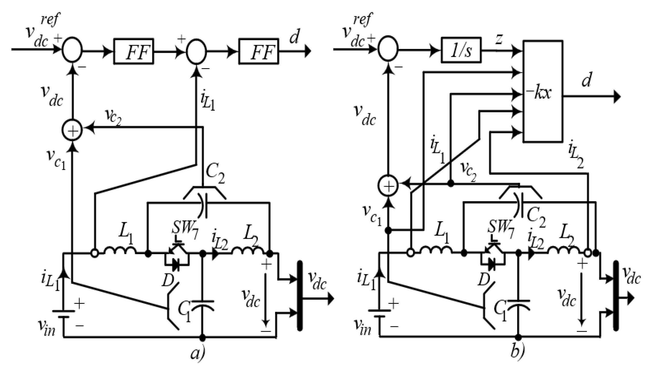
In Figure 2a, the peak DC-link voltage (PDV) and the inductor current $i_{L1}$ are regulated through a cascaded control structure comprising an inner inductor current control loop and an outer PDV control loop. The output of the cascaded controller is the duty cycle d. However, this configuration exhibits performance degradation when the parameters $r_L$, $R_c$, d, and $V_{in}$ vary, thereby affecting the DC-link voltage supplied to the inverter and the inductor current [22].

To overcome these limitations, this paper proposes a linear quadratic integral (LQI) control strategy for PDV regulation under disturbances and parameter variations. The PDV $v_{dc}$ is selected as the system state of the QZS converter, while d serves as the control input, as shown in Figure 2b.

The objective of the proposed control strategy is to ensure that the PDV $v_{dc}$ accurately tracks its reference value, thereby providing a stable DC supply for the inverter [22]. This paper proposes a linear quadratic integral (LQI) control strategy for DC-link voltage regulation under disturbance conditions. Accordingly, we define

$$z={\int }_0^t\left(v_C^{ref}-v_C\right)d\tau$$

(34)

By augmenting (33) with the extended state z, the following expression is obtained:

$${\dot{x}}_a=A_a{x}_a+B_{a}d+E_a\xi +V_a{v}_C^{ref}$$

(35)

where $x_a={\left[\begin{array}{ccccc}{i}_{L_1}& i_{L_2}& v_{c_1}& v_{c_2}& z\end{array}\right]}^T$

$$\begin{array}{cc}\hfill A_a& =\left[\begin{array}{cc}A& 0\\ -C& 0\end{array}\right];B_a^T=\left[\begin{array}{cc}B& 0\end{array}\right];E_a^T=\left[\begin{array}{cc}E& 0\end{array}\right];\hfill \\ \hfill V_a& =\left[\begin{array}{ccccc}0& 0& 0& 0& 1\end{array}\right]\hfill \end{array}$$

The LQI performance index is

$$J={\int }_0^{\infty }\left(x_a^T{Q}_a{x}_a+d^{T}Rd\right)dt$$

(36)

where $Q_a=\mathrm{diag}(10,1,50,50),R=0.01$; the optimal control law is $d=-k{x}_a$, with $k=\left[\begin{array}{ccccc}{k}_{i_{L_1}}& k_{i_{L_2}}& k_{v_{c_1}}& k_{v_{c_2}}& k_z\end{array}\right]$. The optimal gain coefficients k of the LQI controller are defined as follows: $k_{i_{L_1}}$ and $k_{i_{L_2}}$ denote the gains associated with the inductor currents $i_{L_1}$ and $i_{L_2}$, respectively. Similarly, $k_{v_{c_1}}$ and $k_{v_{c_2}}$ correspond to the capacitor voltages $v_{c_1}$ and $v_{c_2}$, respectively. Finally, $k_z$ represents the gain of the integral state associated with the capacitor voltage error $C_1$.

5. Simulation Results for the PZI Control System

5.1. Simulation Results of the Peak of DC-Link Voltage (PDV) in the QZS Scheme

The DC voltage supplied to the inverter is provided through the quasi-Z-source (QZS) network, which functions both as a filtering stage and as a voltage boosting/buck-boosting unit to regulate the DC voltage delivered to the PMSM drive. The proposed PDV controller and the motor speed controller are evaluated through simulation in this section. The parameters of the QZS network used in the simulation of the LQI-based DC-link voltage control are adopted from [22] and are given as follows: ${\overline{I}}_{L_1}$ and ${\overline{I}}_{L_2}$ are the average values of inductor currents through $L_1$ and $L_2$, respectively; the average value of load current ${\overline{I}}_l=0.8$ A;

the switching frequency $f_{sf}=5$ kHz; and ${\overline{I}}_{L_1}$ = ${\overline{I}}_{L_2}$= $0.6$ A. The average value of duty cycle $\overline{D}$ $=0.4$; the two inductors of the QZS are $L_1$ and $L_2$, respectively, and $L_1=L_2=L=0.6\times {10}^{-4}$ H. The two capacitors in the QZS network are $C_1$ and $C_2$, and $C_1=C_2=0.6\times {10}^{-4}$ F. The stator inductance of the PMSM is assumed to be equal to the inductance in the $dq$-axis reference frame, $L_d=L_q=L_l=8.5$ mH. Furthermore, the stator resistance of the motor is used in this system: $R_l=R_s=2.7$ $\mathsf{\Omega }$. Finally, the voltage of the battery source $V_{in}$ supplied to the QZS network is given by $V_{in}=40$ V.

The LQI controller gains are designed following Section 4.2 and the simulation results are as follows. The optimal gain coefficients k of the LQI controller are defined as follows: $k_{i_{L_1}}=0.5$ and $k_{i_{L_2}}=0.5$; $k_{v_{c_1}}=1.2$ and $k_{v_{c_2}}=1.2$. Finally, $k_z=0.1$.

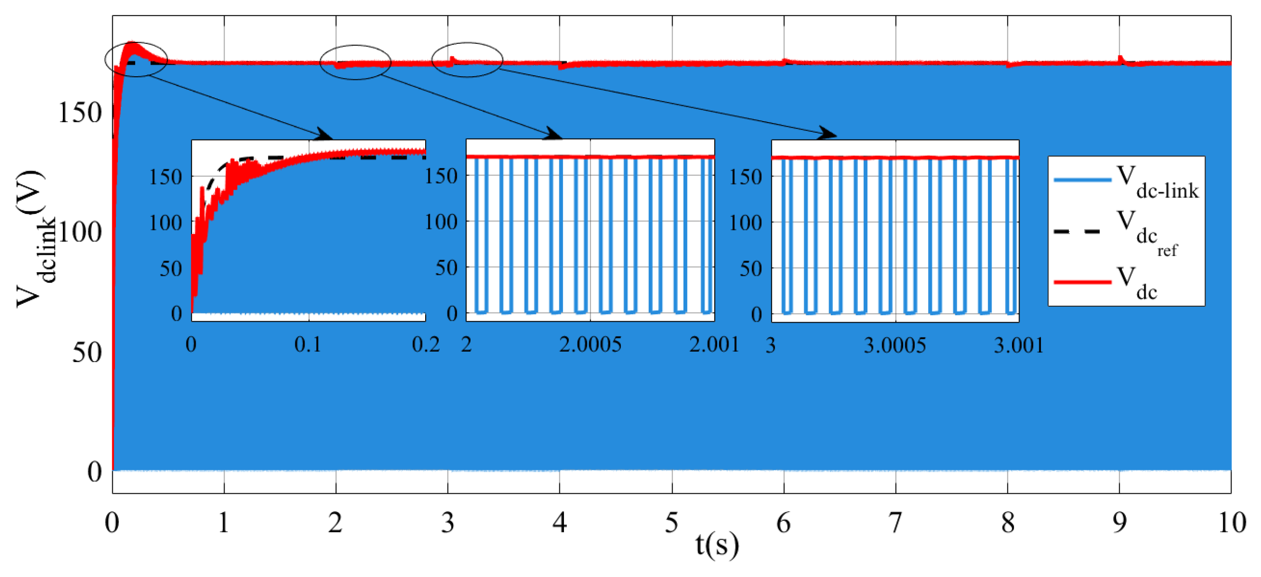
To evaluate the performance of the proposed LQI controller for PDV regulation, the input voltage $V_{in}$ is varied, while the DCV is required to track its reference value. In addition, the influence of disturbance currents on the PDV control performance is investigated. All of the aforementioned scenarios are examined through simulation, as shown in Figure 3. During the time interval from 2.0001 s to 2.002 s, the DCV decreases due to the reduction in $V_{in}$ at time 2 s and 3 s, as illustrated in Figure 4a).

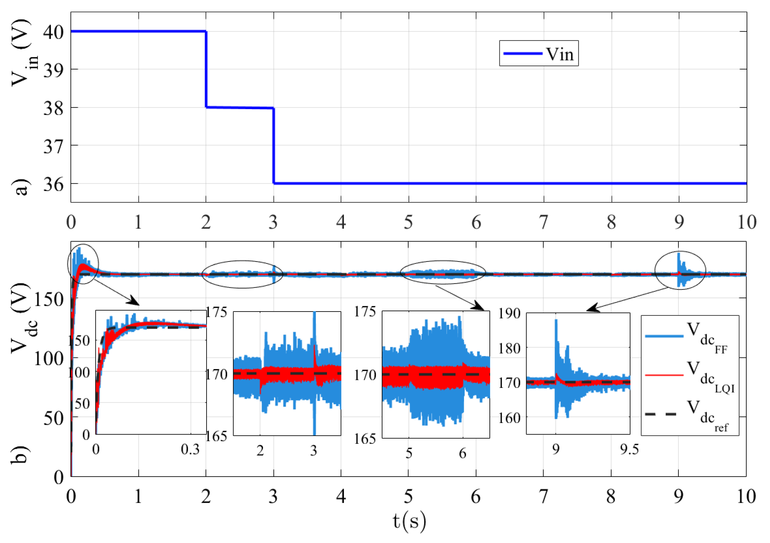
As shown in Figure 4, $V_{in}$, the input voltage, decreases over time. Specifically, $V_{in}$ is maintained at 40 V from 0 s to 2 s. At 2 s, the drop in $V_{in}$ is 38 V. Subsequently, from 2 s to 5 s, $V_{in}$ further decreases to 36 V, as illustrated in Figure 4a).

The linear quadratic integral (LQI) controller is employed for PDV regulation as described in Section 4.2 ensuring that the DCV consistently tracks its 170 V reference, as shown in Figure 4b. The DCV is boosted from 40 V to 170 V, as shown in Figure 4b, and this DCV is regulated and maintained at 170 V. Even when the input voltage $V_{in}$ varies, the DCV, regulated by the proposed LQI controller, remains stabilized at 170 V through the DC-link closed-loop control system illustrated in Figure 2.

5.2. Simulation Results of PMSM Speed Control

PMSM speed control plays a critical role in all-electric aircraft systems, particularly in terms of safety, reliability, and stability under load disturbances, voltage fluctuations, and wind gust conditions [32]. In this paper, an online adaptive optimal tracking control strategy for PMSM speed regulation is proposed as shown in Algorithm 1. The effectiveness of the proposed control scheme is validated through MATLAB-based simulations conducted using MATLAB R2024a. The proposed OAC strategy for PMSM speed control is implemented with the following controller parameters: the convergence gain for the control weight update law is ${\alpha }_u=0.15$; the convergence gain for the disturbance weight update law is ${\alpha }_n=0.1$; and the convergence gain for the critic weight update law is ${\alpha }_{\Lambda }=0.1$. The weight update laws for the control, disturbance, and critic are terminated when their respective estimation errors fall below the prescribed threshold ${ϵ}_m$, where ${ϵ}_m=1\times {10}^{-4}$ for $m\in \Lambda ,u,n$. The parameter $\rho$, representing the design coefficient associated with the OAC scheme, is chosen as $\rho =0.8$. The control weighting coefficient in the control law $\widehat{u}$ is $R=1$.

Algorithm 1. Online adaptive optimal tracking control algorithm.

Initialization:

1. Set initial weights: ${\widehat{W}}_{\Lambda }={\widehat{W}}_u={\widehat{W}}_n=0$.

2. Set initial states: $\widehat{u}=\widehat{n}=\widehat{\Lambda }=0$.

3. Set convergence thresholds: ${ϵ}_{\Lambda }={ϵ}_u={ϵ}_n={10}^{-4}$.

4. Select parameters: ${\mathsf{\Psi }}_{\Lambda },{\alpha }_u,{\alpha }_n,\gamma ,Q,$ and R are positive.

5. Set iteration counter $k=0$ and maximum steps $k_{max}$.

Repeat:

6. Compute the approximated value function:

${\widehat{\Lambda }}^{\left(k\right)}\leftarrow {({\widehat{W}}_{\Lambda }^{\left(k\right)})}^{\top }{\mathsf{\Psi }}_{\Lambda }$

7. Update control and disturbance policies:

${\widehat{u}}^{\left(k\right)}\leftarrow -{\displaystyle \frac{1}{2\rho }}{R}^{-1}g{\left(e\right)}^{\top }\mathsf{\nabla }{\mathsf{\Psi }}_{\Lambda }{\left(e\right)}^{\top }{\widehat{W}}_u^{\left(k\right)}$

${\widehat{n}}^{\left(k\right)}\leftarrow {\displaystyle \frac{1}{2{\gamma }^2}}k{\left(e\right)}^{\top }\mathsf{\nabla }{\mathsf{\Psi }}_{\Lambda }{\left(e\right)}^{\top }{\widehat{W}}_n^{\left(k\right)}$

8. Apply ${\widehat{u}}^{\left(k\right)}$ and ${\widehat{n}}^{\left(k\right)}$ to system (11) and measure state e.

Weight Update:

9. Update critic weights ${\widehat{W}}_{\Lambda }^{(k+1)}$ using (30).

10. Update actor weights ${\widehat{W}}_u^{(k+1)}$ using (31).

11. Update disturbance weights ${\widehat{W}}_n^{(k+1)}$ using (32).

12. $k\leftarrow k+1$

Until$(k>k_{max})$or convergence condition met:

$\parallel {\widehat{W}}_{\Lambda }^{\left(k\right)}-{\widehat{W}}_{\Lambda }^{(k-1)}\parallel <{ϵ}_{\Lambda }$ and

$\parallel {\widehat{W}}_u^{\left(k\right)}-{\widehat{W}}_u^{(k-1)}\parallel <{ϵ}_u$ and

$\parallel {\widehat{W}}_n^{\left(k\right)}-{\widehat{W}}_n^{(k-1)}\parallel <{ϵ}_n$

The nominal parameters of the PMSM used in the all-electric aircraft control system are specified as follows: rated power $P_n=400$ W and rated speed of the PMSM $\omega =3000$ rpm; rated voltage is $v_n$; rate torque $T_L=1.27$ N·m; permanent magnet flux ${\psi }_f=$$0.0615$ Wb; inertia moment of the motor $J=31.69\times {10}^{-6}$ kg·m²; pole pair $n_p=4$; stator resistance of the motor $R_s=2.7$ $\mathsf{\Omega }$; rotor inductance expressed in the $dq$ reference frame $L_d=L_q=8.5$ mH; and viscous friction coefficient $B=52.79\times {10}^{-6}$ Ns·m⁻².

$${\mathsf{\Psi }}_{\Lambda }(e_{\omega },e_{i_d},e_{i_q})={\left[\begin{array}{cccccc}{e}_{\omega }^2& e_{\omega }{e}_{i_d}& e_{\omega }{e}_{i_q}& e_{i_d}^2& e_{i_d}{e}_{i_q}& e_{i_q}^2\end{array}\right]}^T;$$

$${\displaystyle \frac{\partial {\mathsf{\Psi }}_{\Lambda }}{\partial e}}=\mathsf{\nabla }{\mathsf{\Psi }}_{\Lambda }(e_{\omega },e_{i_d},e_{i_q})=\left[\begin{array}{ccc}{\displaystyle \frac{\partial {\mathsf{\Psi }}_{\Lambda }}{\partial e_{\omega }}}& {\displaystyle \frac{\partial {\mathsf{\Psi }}_{\Lambda }}{\partial e_{i_d}}}& {\displaystyle \frac{\partial {\mathsf{\Psi }}_{\Lambda }}{\partial e_{i_q}}}\end{array}\right]$$

$${\widehat{W}}_u={\left[\begin{array}{ccc}{\widehat{W}}_{v_{iq}}& {\widehat{W}}_{v_{v_d}}& {\widehat{W}}_{v_{v_q}}\end{array}\right]}^T;{\widehat{W}}_{\Lambda }={\left[\begin{array}{ccc}{\widehat{W}}_{iq}& {\widehat{W}}_{v_d}& {\widehat{W}}_{v_q}\end{array}\right]}^T;$$

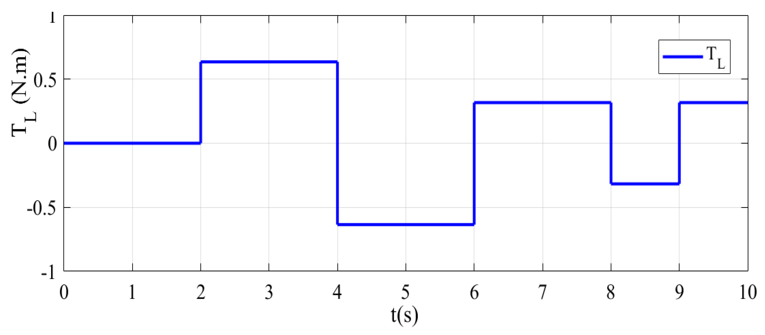
The load torque $T_L$ is varied during the simulation, and its profile is shown in Figure 5. The load torque applied to the motor shaft is maintained at 0 N·m from 0 s to 0.25 s. It is then step-increased to 1.27/4 N·m during the interval from 0.25 s to 1 s. Subsequently, from 1 s to 2.5 s, the load torque is further increased, and from 2.5 s onward, it is maintained at 1.27 N·m.

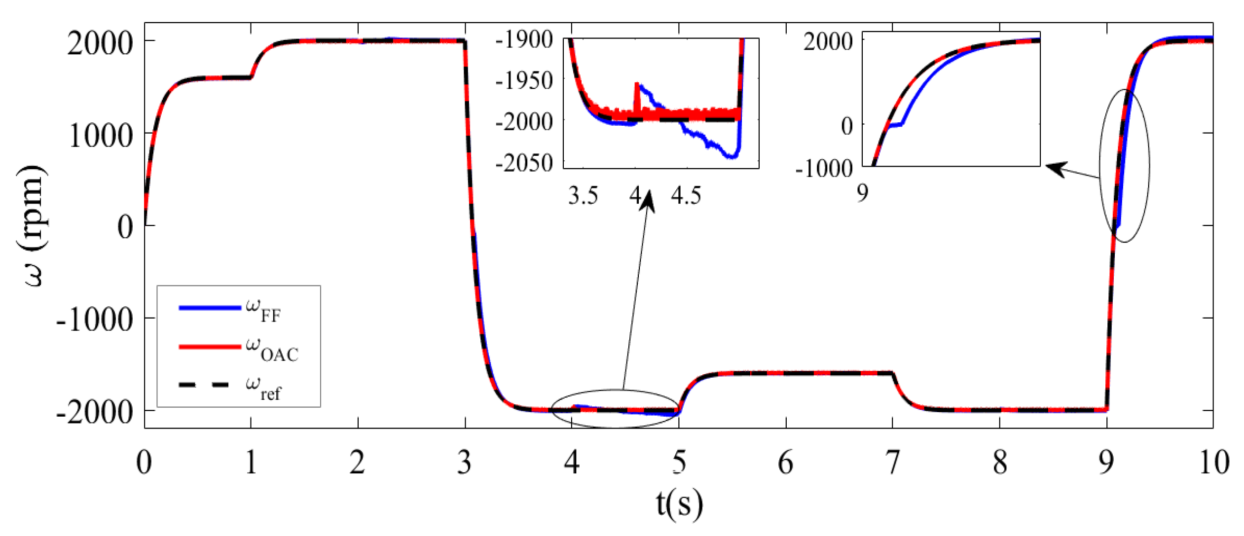
Figure 6 shows that when the load torque is increased by a step from 1.27/4 N·m to 1.27/3 N·m at t = 1 s, the PMSM speed controlled by the proposed OAC strategy continues to track its reference value in a stable manner. In contrast, under the conventional PI-based speed control strategy, the motor speed exhibits noticeable tracking degradation. These results demonstrate the effectiveness and robustness of the proposed OAC strategy.

In addition to load torque variations, this paper also considers the effect of control voltage disturbances. In this study, the disturbance signal is generated using the Uniform Random Number block, which produces a uniformly distributed random signal, and is added to the control signal, namely, the $dq$-axis voltage. When this disturbance signal is introduced, the motor speed is affected.

During the time interval from $4\mathrm{s}$ to $5\mathrm{s}$, a uniformly distributed random disturbance signal with an amplitude of $0.1$ is injected. As a result, the motor speed response with the OAC controller (red line) quickly tracks its reference speed, whereas with the FF controller (blue line), the motor speed fails to track the reference speed effectively and exhibits a deviation of approximately $-45\mathrm{rpm}$ from its reference value.

Furthermore, the stator resistance and inductance components of the motor, namely, $R_s$ and $L_s$, are reduced by $10\%$ after $9\mathrm{s}$ of motor operation. As shown in Figure 6, from the instant of $9.2\mathrm{s}$, the motor speed using the OAC method tracks its reference speed very well. In contrast, with the FF method, the speed tracking performance is poor. This can be clearly observed in the enlarged view of Figure 6 during the time interval from $9\mathrm{s}$ to $10\mathrm{s}$.

These results demonstrate that the OAC controller can robustly track the reference speed and adapt effectively in the presence of disturbances.

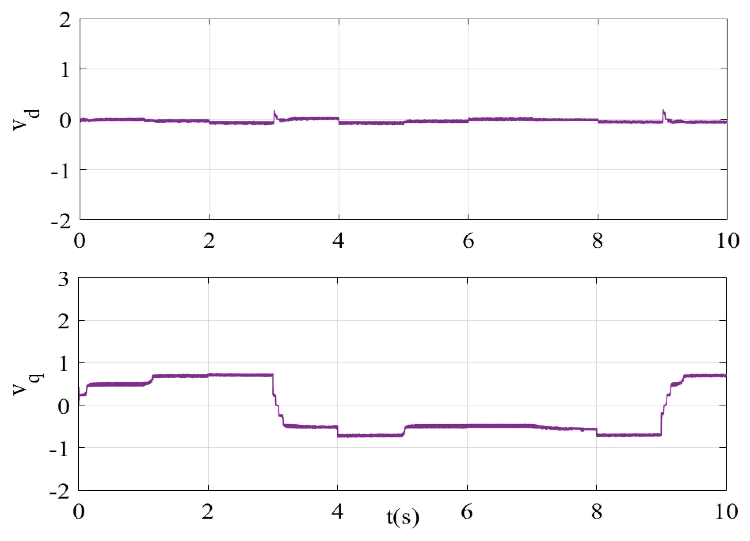
The signal control inputs are the $dq$-axis voltages: $v_d$ and $v_q$, as illustrated in Figure 1. The d-axis voltage $v_d$ remains approximately zero, indicating proper decoupling, while the q-axis voltage $v_q$ varies in response to changes in PMSM speed, load torque, and DVP, as shown in Figure 7.

6. Conclusions

This paper has presented an optimal tracking control framework for a PMSM drive system integrated with a quasi-Z-source (QZS) inverter for all-electric aircraft applications. The proposed framework combines an online adaptive optimal control (OAC) strategy for PMSM speed tracking and a linear quadratic integral (LQI) controller for peak DC-link voltage (PDV) regulation, with the aim of improving dynamic performance, robustness, and energy efficiency under nonlinear dynamics, parameter uncertainties, and external disturbances.

For the PMSM speed control loop, the motor dynamics were formulated as a nonlinear strict-feedback system, and augmented feedforward control signals were incorporated to establish a novel optimal control structure. Based on the approximate solution of the Hamilton–Jacobi–Isaacs (HJI) equation, a saturated adaptive optimal control law was developed using an online approximator and an integral reinforcement learning (IRL) algorithm. The obtained results confirmed that the proposed OAC strategy achieves accurate speed tracking, fast transient response, and strong robustness against load torque disturbances, input voltage variations, and unmodeled dynamics. Compared with the conventional PI controller, the proposed controller provides superior tracking accuracy and disturbance rejection capability.

For the DC-link voltage regulation loop, an LQI-based PDV control strategy was designed to stabilize the inverter input voltage under varying operating conditions. Since the battery voltage in all-electric aircraft systems is typically lower than the required PMSM drive voltage, the QZS converter was employed to provide voltage boosting capability. By integrating the QZS topology with the proposed LQI controller, stable and accurate DC-link voltage regulation was achieved despite fluctuations in the input voltage, load disturbances, and continuously varying motor speed. The results verified that the proposed PDV regulation strategy effectively suppresses voltage oscillations and enhances the reliability of the integrated drive system.

Overall, the proposed PMSM–QZS closed-loop control framework exhibits effective and robust performance in the presence of disturbances and parameter uncertainties. The proposed approach demonstrates strong potential for practical implementation in all-electric aircraft systems requiring high-performance motor drives, reliable operation, and improved energy efficiency.

Future work will focus on experimental validation using real-time hardware platforms and hardware-in-the-loop (HIL) implementation for all-electric aircraft applications. In addition, advanced intelligent control techniques, including deep reinforcement learning and fault-tolerant control strategies, will be investigated to further improve system adaptability, operational reliability, and energy management capability under practical operating conditions.

References

1. Davari, S.A.; Mousavi, M.S.; Nikmaram, B.; Flores-Bahamonde, F.; Wang, F.; Wheeler, P.; Rodriguez, J. Sensorless Model-Free Predictive Control of Permanent Magnet Synchronous Motor. IEEE Trans. Ind. Electron. 2026, 73, 1570–1581. [Google Scholar] [CrossRef]
2. Ding, B.; Lu, Y.; Lai, C.; Feng, G. Single Open-Phase Fault Tolerant Control of Salient Dual Three-Phase PMSMs With Maximized Torque to Total Loss Ratio Considering Peak Phase Current Limit. IEEE Trans. Ind. Electron. 2025, 72, 6852–6864. [Google Scholar] [CrossRef]
3. Karboua, D.; Belgacem, T.; Khan, Z.H.; Kellal, C. Robust performance comparison of PMSM for flight control applications in more electric aircraft. PLoS ONE 2023, 18, e0283541. [Google Scholar] [CrossRef]
4. Basappa, M.H.; Viswanathan, P. Direct torque control for permanent magnet synchronous motor using golden eagle optimized ANFIS. Int. J. Intell. Eng. Syst. 2022, 15, 499–508. [Google Scholar] [CrossRef]
5. Abu-Rub, H.; Iqbal, A.; Guzinski, J. High Performance Control of AC Drives with MATLAB/Simulink, 2nd ed.; John Wiley and Sons: Hoboken, NJ, USA, 2021. [Google Scholar]
6. Pham, C.-T.; Huu, C.T.N.; Tran, Q.-K.; Thien, T.V.; Nguyen, D.T.-H. Adaptive backstepping sliding mode control for speed of PMSM and DC-link voltage in bidirectional quasi Z-source inverter. In Proceedings of the 2023 International Conference on Intelligent Systems and Computer Networks (INSICOM); Springer: Cham, Switzerland, 2023; pp. 185–202. [Google Scholar]
7. Tan, L.N.; Pham, T.C. Optimal tracking control for PMSM with partially-unknown dynamics, saturation voltages, torque and voltage disturbances. IEEE Trans. Ind. Electron. 2021, 69, 3481–3491. [Google Scholar] [CrossRef]
8. Wongyai, P.; Pakdeeto, J.; Chaicharoenaudomrung, K.; Areerak, K.; Areerak, K. The Controller Design of Quasi-Z-Source Inverter for PV-Rooftop System Using Fuzzy Controller. ECTI Trans. Electr. Eng. Electron. Commun. 2023, 21, 251459. [Google Scholar]
9. Agung, R.; Syamsiana, I.N.; Sumari, A.D.W. PSO-Based PI Parameter Optimization for PMSM Speed Control Using Field-Oriented Control. Tekno J. 2026, 16, 307–319. [Google Scholar]
10. Umaru, K.; Ritah, N.; Rodney, M.; Nansukusa, Y.; Asikuru, S.; Ochima, N.; Mutaburura, P.; Zaina, K. Fuzzy-PID Control Design and Performance Analysis for PMSM Drives in Electric Vehicles. J. Eng. Technol. Appl. Sci. 2025, 7, 127–148. [Google Scholar] [CrossRef]
11. Li, Y.; Zhang, H.; Wang, J. Deep Reinforcement Learning-Based Control method for Permanent Magnet Synchronous Motor Drives. IEEE Access 2024, 12, 123456–123468. [Google Scholar]
12. Vrabie, D.; Vamvoudakis, K.G.; Lewis, F.L. Optimal Adaptive Control and Differential Games by Reinforcement Learning Principles; IET Control Theory and Applications; Institution of Engineering and Technology (IET): London, UK, 2013. [Google Scholar]
13. Farbood, M.; Echreshavi, Z.; Shasadeghi, M. Parameter Varying Model Predictive Control Based on T–S Fuzzy Model Using QP Approach: A Case Study. Iran. J. Sci. Technol. Trans. Electr. Eng. 2019, 43, 269–276. [Google Scholar] [CrossRef]
14. Palangari, M.F.; Echreshavi, Z.; Messilem, M.A.; Carli, R.; Mobayen, S.; Zampieri, S. Two-Stage Event-Triggered Model Predictive Power Control of EV Charging Stations With V2G Capability. IEEE Trans. Transp. Electrif. 2025, 12, 797–810. [Google Scholar] [CrossRef]
15. Farbood, M.; Echreshavi, Z.; Shasadeghi, M.; Mobayen, S.; Skruch, P. Disturbance Observer-Based Data Driven Model Predictive Tracking Control of Linear Systems. IEEE Access 2023, 11, 88597–88608. [Google Scholar] [CrossRef]
16. Vamvoudakis, K.G.; Lewis, F.L. Online solution of nonlinear two-player zero-sum games using synchronous policy iteration. Int. J. Robust Nonlinear Control 2012, 22, 1460–1483. [Google Scholar] [CrossRef]
17. Vamvoudakis, K.G.; Kokolakis, N.-M.T. Synchronous Reinforcement Learning-Based Control for Cognitive Autonomy. Found. Trends Syst. Control 2020, 8, 1–175. [Google Scholar]
18. Jahns, T.M.; Soong, W.L. Electric Machines for Electric Vehicle Applications. IEEE Trans. Ind. Appl. 2022, 59, 1263–1272. [Google Scholar]
19. Hota, A.; Agarwal, V. Novel Three-Phase H10 Inverter Topology with Zero or Constant Common-Mode Voltage for Three-Phase Induction Motor Drive Applications. IEEE Trans. Ind. Electron. 2022, 69, 7522–7525. [Google Scholar] [CrossRef]
20. Poorfakhraei, A.; Narimani, M.; Emadi, A. A Review of Modulation and Control Techniques for Multilevel Inverters in Traction Applications. IEEE Access 2021, 9, 24187–24204. [Google Scholar] [CrossRef]
21. Tan, L.N.; Cong, T.P.; Cong, D.P. Neural Network Observers and Sensorless Robust Optimal Control for Partially Unknown PMSM With Disturbances and Saturating Voltages. IEEE Trans. Power Electron. 2021, 36, 12045–12056. [Google Scholar] [CrossRef]
22. Lakhe, R.K.; Chaoui, H.; Alzayed, M.; Liu, S. Universal control of permanent magnet synchronous motors with uncertain dynamics. Actuators 2021, 10, 49. [Google Scholar] [CrossRef]
23. Liu, D.; Xue, S.; Zhao, B.; Luo, B.; Wei, Q. Adaptive Dynamic Programming for Control: A Survey and Recent Advances. IEEE Trans. Syst. Man Cybern. Syst. 2021, 51, 142–160. [Google Scholar] [CrossRef]
24. Vamvoudakis, K.G.; Lewis, F.L. Online Actor–Critic Reinforcement Learning for Optimal Control of Continuous-Time Systems. Automatica 2010, 46, 878–888. [Google Scholar] [CrossRef]
25. Vamvoudakis, K.G.; Lewis, F.L. Online adaptive algorithm for optimal control with integral reinforcement learning. Int. J. Robust Nonlinear Control 2014, 24, 2686–2710. [Google Scholar] [CrossRef]
26. Wang, D.; Gao, N.; Liu, D.; Li, J.; Lewis, F.L. Recent Progress in Reinforcement Learning and Adaptive Dynamic Programming for Advanced Control Applications. IEEE/CAA J. Autom. Sin. 2024, 11, 18–36. [Google Scholar] [CrossRef]
27. Xu, Z.; Kontoudis, G.P.; Vamvoudakis, K.G. Online and Robust Intermittent Motion Planning in Dynamic and Changing Environments. IEEE Trans. Neural Netw. Learn. Syst. 2024, 35, 17425–17439. [Google Scholar] [CrossRef] [PubMed]
28. Zhao, B.; Liu, D.; Luo, C. Reinforcement Learning-Based Optimal Stabilization for Unknown Nonlinear Systems Subject to Inputs with Uncertain Constraints. IEEE Trans. Neural Netw. Learn. Syst. 2020, 31, 4330–4340. [Google Scholar] [CrossRef]
29. Siwakoti, Y.P.; Peng, F.Z.; Blaabjerg, F.; Loh, P.C.; Town, G.E.; Yang, S. Impedance-Source Networks for Electric Power Conversion Part II: Review of Control and Modulation Techniques. IEEE Trans. Power Electron. 2015, 30, 1887–1906. [Google Scholar] [CrossRef]
30. Liu, Y.; Abu-Rub, H.; Xue, Y.; Tao, F. A Discrete-Time Average Model-Based Predictive Control for a Quasi-Z-Source Inverter. IEEE Trans. Ind. Electron. 2018, 65, 6044–6054. [Google Scholar] [CrossRef]
31. Li, S.; Liu, Z. Speed Control for PMSM Servo System Using Predictive Functional Control and Extended State Observer. IEEE Trans. Ind. Electron. 2012, 59, 1171–1183. [Google Scholar] [CrossRef]
32. Pham, C.T.; Tran, Q.K.; Huu, C.T.N. Comparative analysis of speed control strategies for five-phase PMSM in propulsion systems of two-seater all-electric aircraft. Int. J. Sustain. Aviat. 2025, 11, 217–236. [Google Scholar] [CrossRef]
Figure 1. The overall architecture of the proposed online adaptive optimal PMSM speed control integrated with the PZI topology.
Machines 14 00642 g001
Figure 2. (a) The block diagram of the FF controller, (b) The block diagram of the LQI, controller.
Machines 14 00642 g002
Figure 3. The DCV V d c and the DCV peak V d c p e a k .
Machines 14 00642 g003
Figure 4. (a) The V i n . (b) The DVP V d c ; the DVP reference is V d c r e f .
Machines 14 00642 g004
Figure 5. Load torque T L changes over time.
Machines 14 00642 g005
Figure 6. The speed of the PMSM response with FF and OAC.
Machines 14 00642 g006
Figure 7. The control input v d q -axis with the OAC controller.
Machines 14 00642 g007
Disclaimer/Publisher’s Note: The statements, opinions and data contained in all publications are solely those of the individual author(s) and contributor(s) and not of MDPI and/or the editor(s). MDPI and/or the editor(s) disclaim responsibility for any injury to people or property resulting from any ideas, methods, instructions or products referred to in the content.