1. Introduction
Rotating machinery is widely used in numerous industrial applications and plays a key role in power transmission, energy conversion, and mechanical motion generation [
1,
2]. Its operational stability directly affects the efficiency and safety of production systems. Among various mechanical components, rolling bearings are critical for sustaining rotational motion [
3]. They are frequently exposed to harsh operating environments, including heavy loads, variable speeds, and complex vibration conditions. Such environments make bearings prone to localized damage, which often develops gradually and is difficult to detect in real time. Once incipient defects propagate to a critical level, catastrophic breakdowns may result, leading to unexpected downtime, substantial economic losses, and even safety hazards [
4,
5]. Therefore, early and reliable detection of bearing faults is fundamental to stable operation and to the advancement of intelligent and sustainable manufacturing [
6,
7].
The rapid development of Industry 4.0 and intelligent manufacturing has increased the demand for advanced fault diagnosis technologies. Over the past decades, various diagnostic methods have been applied to bearing damage detection. In addition to vibration-based diagnosis, temperature monitoring has shown that measured temperature profiles are correlated with internal friction conditions and can effectively reflect bearing health [
8,
9]. Recent advances in artificial intelligence, especially deep learning, have further improved fault diagnosis by enabling automatic feature learning from large-scale labeled datasets [
10]. For example, CNN-based, CNN-LSTM-based, graph-neural-network-based, residual-shrinkage, and envelope-spectrum-based models have been developed for rotating machinery and bearing fault diagnosis [
11,
12,
13,
14,
15]. Despite these advances, acquiring sufficient fault data in real industrial environments remains difficult because machinery usually operates stably for long periods, while severe failures often trigger immediate shutdown for safety. The increasing complexity of industrial systems further restricts fault data acquisition. Therefore, developing accurate diagnostic methods under limited or unavailable fault samples remains an important research issue [
16].
Given the dependence of neural network models on large-scale labeled data, existing fault diagnosis methods for data-scarce scenarios can generally be divided into transfer-learning-based and few-shot-learning-based approaches. Transfer learning methods aim to transfer diagnostic knowledge from data-rich source domains to target domains with limited samples, thereby improving performance under insufficient fault data [
17]. For example, domain adaptation, joint distribution alignment, federated transfer learning, and optimized deep belief networks have been investigated to reduce source–target distribution discrepancies and enhance cross-domain diagnosis [
18,
19,
20,
21]. In addition, convolutional autoencoder-based transfer frameworks have been used to learn domain-invariant representations through correlation alignment and domain classification losses [
22]. Although these methods improve diagnostic performance under varying operating conditions and sensor domains, they still rely on the availability of related source-domain data and may suffer from negative transfer when the domain discrepancy is large.
Few-shot learning methods aim to recognize unseen fault categories using only a few labeled samples per class. These methods commonly rely on metric learning, prototype networks, meta learning, or Transformer-based architectures to improve generalization under limited fault data. For example, graph-based few-shot learning has been used to propagate label information from a few labeled samples to unlabeled data [
23], while meta-transfer learning and prior-knowledge-guided strategies have been developed to address varying operating conditions and improve feature adaptability [
24,
25]. To further enhance robustness, asymmetric loss functions and prototype-based networks have also been introduced for noisy labels, limited samples, and multi-source diagnostic scenarios [
26,
27]. Although these methods reduce the dependence on abundant labeled fault data, they still require a small number of real fault samples for each target class. Their performance may deteriorate when fault patterns are highly complex or when only healthy data are available during training. Therefore, alternative diagnostic strategies are still needed for scenarios with zero or extremely limited real fault samples.
Although transfer-learning-based and few-shot-learning-based methods have alleviated data scarcity in fault diagnosis, important limitations remain. Transfer learning depends on related source domains and may suffer from negative transfer under large source–target distribution discrepancies. Few-shot learning improves generalization with limited labeled fault samples, but its performance may degrade when fault patterns are complex or when no real fault samples are available for training. To address this stricter setting, this study proposed a simulation-driven bearing fault diagnosis framework under fault-free training conditions. The framework focused on a practical zero-real-fault-sample scenario, where typical bearing fault categories were known from prior mechanical knowledge, but real fault samples were unavailable for training. Theoretical fault characteristic frequencies, estimated from bearing geometry and rotational speed, were used to guide pseudo-fault synthesis rather than being learned from real fault data. Pseudo-fault samples were generated by superimposing periodic impulse–resonance responses onto healthy vibration signals. Wavelet packet decomposition and envelope spectrum analysis were then used to extract fault-sensitive time–frequency features. These features were fed into HCANet, where WPD-based sub-band representations were coupled with grouped convolution and grouped attention mechanisms. Central Clustering Loss was further introduced to enhance intra-class compactness, inter-class separability, and pseudo-to-real feature transferability. The primary contributions of this work can be summarized as follows:
- (1)
This study developed a simulation-driven framework for zero-real-fault-sample bearing diagnosis using healthy signals and synthesized pseudo-fault samples.
- (2)
The pseudo-fault synthesis process was designed to follow the physical mechanism of localized bearing defects by generating periodic impulse–resonance responses governed by theoretical fault characteristic frequencies.
- (3)
Two-level WPD sub-band representations were coupled with grouped convolution and grouped attention in HCANet, enabling sub-band-specific feature extraction and inter-band dependency modeling.
- (4)
Central Clustering Loss was introduced to enhance pseudo-to-real feature transferability by improving intra-class compactness and inter-class separability in the embedding space.
The remaining sections are organized as follows.
Section 2 presents the theoretical background of wavelet packet decomposition and the multi-head attention mechanism.
Section 3 introduces the proposed simulation-driven framework for bearing fault diagnosis when fault samples are unavailable for training.
Section 4 demonstrates the effectiveness of the proposed method through experiments on two benchmark bearing datasets. Finally,
Section 5 concludes the paper and outlines possible directions for future research.
3. Methods
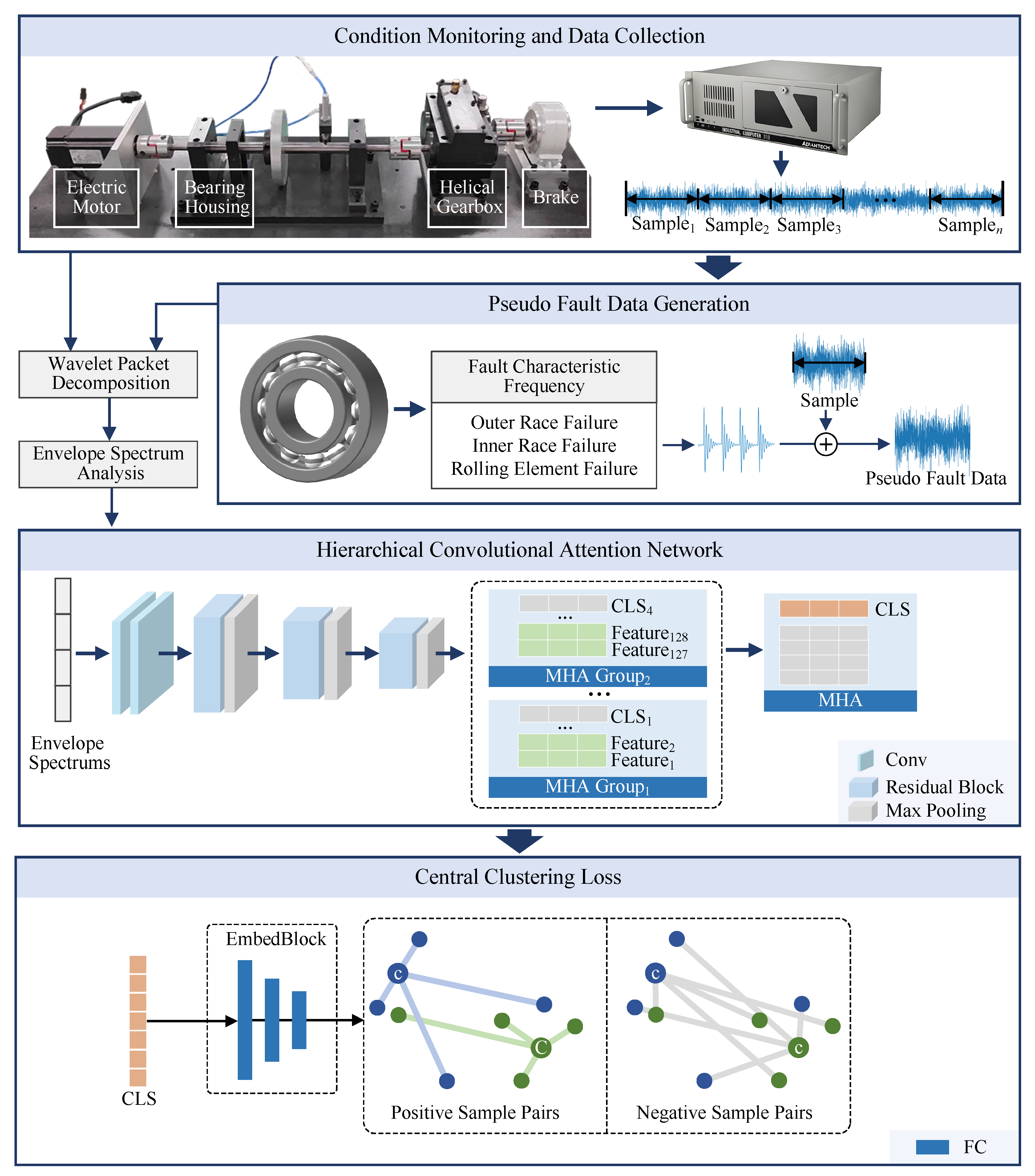
A simulation-based framework for bearing diagnosis without faulty training samples is developed in this section and summarized in
Figure 2. In real applications, data acquired from normal operating conditions are usually sufficient, whereas fault data remain limited because real failures occur rarely and artificial fault induction involves considerable cost and safety concerns. Accordingly, the problem addressed here assumes that model training is conducted using only normal-condition data, while measurements from faulty bearings are unavailable. Such conditions not only highlight the challenge of data scarcity but also increase the risk of poor generalization when models are applied to real faults.
3.1. Simulation-Driven Pseudo-Fault Synthesis
Obtaining sufficient fault samples in real industrial environments is inherently difficult owing to the low occurrence frequency of failures, the expense of fault induction, and the associated safety risks. In contrast, healthy vibration data are typically accessible under multiple operating conditions. To overcome this imbalance, a simulation-driven pseudo-fault synthesis strategy is proposed in this study. It should be emphasized that the proposed strategy does not directly superimpose sinusoidal characteristic-frequency components onto healthy signals. Instead, the characteristic fault frequencies are used to determine the repetition intervals of localized-defect-induced impulses. These impulses are then modeled as exponentially decaying responses, modulated by the load-zone effect, and finally superimposed onto healthy vibration signals to generate pseudo-fault samples. Therefore, only one pseudo-fault synthesis model is used in this study, namely the periodic impulse–resonance model with load-zone modulation. The overall procedure consists of two key steps: first, estimating the characteristic frequencies associated with different bearing fault types; and second, constructing periodic impulse–resonance responses according to the estimated frequencies. The synthesized pseudo-fault data serve as effective substitutes for real fault samples during training, enabling the development of diagnostic models under fault-free conditions.
3.1.1. Fault Characteristic Frequency Estimation
The vibration response of a rolling bearing is strongly influenced by its geometric configuration and operating state. When a localized defect appears on the outer race, inner race, or rolling element, repeated contact between the defect and the rolling elements gives rise to periodic impulses. These impulses correspond to characteristic fault frequencies, which can be analytically determined from the bearing geometry and shaft rotational speed. Let
denote the shaft rotational frequency,
D the bearing pitch diameter,
d the rolling-element diameter,
z the number of rolling elements, and
the contact angle. On this basis, the characteristic frequencies associated with typical fault locations are given by:
where
,
, and
correspond to the characteristic frequencies associated with outer race defects, inner race defects, and rolling element defects, respectively.
These analytical expressions provide a theoretical reference for embedding simulated fault components into healthy signals. By using the estimated characteristic frequencies, pseudo-fault signals can be synthesized to approximate the spectral signatures of real bearing failures.
3.1.2. Synthesis of Periodic Fault Impulses
Once the characteristic fault frequencies are determined, pseudo-fault signals can be synthesized through periodic impulse responses that replicate the excitation produced by localized defects. When a rolling element passes over a defect, a short duration impact is generated and excites the structural resonance of the bearing and its surrounding components. The resulting vibration can be modeled as a sequence of exponentially decaying impulses repeated at the fault characteristic frequency. Let
,
, and
a denote the fault characteristic frequency, the structural resonance frequency, and the decay constant, respectively. The periodic excitation can be expressed as
where
is the unit step function, which ensures that each impulse decays smoothly over time. The corresponding resonance response is then obtained as
To better reflect practical conditions, the periodic impulses are further shaped by a load-zone modulation function
. This function accounts for the fact that impacts occur predominantly when rolling elements are located within the load-carrying region. The modulation can be approximated by a half-wave rectified sinusoid that is synchronized with the shaft rotational frequency
:
Accordingly, the synthesized pseudo-fault signal is expressed as
where
denotes additive white Gaussian noise used to simulate environmental disturbances. Through this formulation, the pseudo-fault signal consists of three essential components: the periodic impulse train governed by the fault characteristic frequency, the structural resonance of the bearing system, and stochastic noise. These synthesized signals offer a realistic representation of actual bearing fault vibrations and can be used to augment healthy data for training diagnostic models.
3.2. Data Preprocessing
Bearing vibration signals are typically non-stationary, with fault-related components distributed across multiple frequency bands. To capture these discriminative characteristics, this study adopts a time–frequency feature extraction approach that combines wavelet packet decomposition and envelope spectrum (ES) analysis.
3.2.1. WPD-Based Sub-Band Energy Feature Extraction
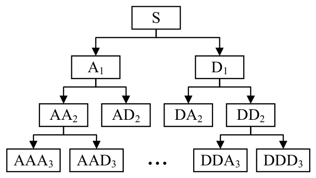
Wavelet Packet Decomposition extends the classical wavelet transform by recursively decomposing both approximation and detail coefficients, thereby producing a complete binary tree structure. This allows for a finer division of the frequency spectrum and provides improved adaptability for analyzing non-stationary signals. At a given node
at decomposition level
j, the corresponding wavelet packet coefficients
are obtained. The associated energy feature is calculated as
where
N is the number of coefficients in node
. Concatenating the energy distribution across selected nodes yields a discriminative feature vector that characterizes the spectral properties of the signal.
3.2.2. Envelope Spectrum
While WPD provided multi-resolution frequency information, envelope analysis was particularly effective in highlighting fault-related periodic impacts. The analytic signal of was obtained using the Hilbert transform , and the signal envelope was calculated as , where denotes the envelope of the signal. The frequency-domain representation of the envelope, namely the envelope spectrum, was then obtained through Fourier transform as . Characteristic fault frequencies and their harmonics appeared as prominent peaks in , serving as reliable indicators of bearing defects. The features extracted from WPD and ES were complementary: WPD captured broadband energy distributions across hierarchical frequency bands, whereas ES emphasized modulation components related to fault impulses. In this study, both feature sets were concatenated to form the final input representation for the neural network, enabling the model to exploit both global frequency structures and localized fault-sensitive information.
In this study, two-level WPD was adopted to obtain four sub-band components. This choice was made by considering the trade-off between frequency resolution, coefficient length, feature stability, and network compatibility. For an L-level WPD, the original signal is decomposed into sub-bands, and the coefficient length of each sub-band is approximately . Given a signal length of , one-level, two-level, and three-level WPD produce sub-band coefficient lengths of 2048, 1024, and 512, respectively. Although three-level WPD provides finer frequency partitioning, the shorter coefficient length may reduce the statistical stability of sub-band energy and envelope-spectrum estimation. Moreover, excessively fine decomposition may split fault-related resonance and modulation components into multiple narrow sub-bands, leading to fragmented fault representations. In contrast, two-level WPD divides the frequency range into four sub-bands, which provides sufficient frequency localization while maintaining a compact and stable feature representation. This setting also matches the four-group convolutional and attention structure of HCANet.
3.3. Hierarchical Convolutional Attention Network
After two levels of wavelet packet decomposition, the raw vibration signal is divided into four equal-bandwidth sub-signals. Their envelope spectra are then used as inputs to the proposed Hierarchical Convolutional Attention Network (HCANet). The design is termed hierarchical because each convolutional layer employs grouped convolutions, where the channels are split into four groups. This enables each group to focus on extracting features from a specific frequency sub-band, thereby reducing redundancy and preserving localized characteristics. The backbone of HCANet is composed of two grouped convolutional layers followed by three residual blocks, each directly connected to a max-pooling operation. Batch normalization (BN) layers are included to stabilize training, while ReLU activation functions introduce nonlinearity. This design progressively compresses the feature dimension while retaining discriminative fault information. The detailed configuration of each stage, including kernel size, number of channels, and grouping strategy, is summarized in
Table 1.
To capture long-range dependencies beyond local convolutions, MHA was applied to the extracted feature maps. The computational complexity of full attention is , which becomes prohibitive for long sequences. To reduce this computational burden, HCANet employed grouped attention by dividing the feature map into subgroups. The number of attention groups was determined by the two-level WPD structure, which decomposed the original vibration signal into four sub-band components. Therefore, each attention group corresponded to one frequency sub-band representation, allowing the model to preserve sub-band-specific fault information while reducing the computational cost of full attention. Each subgroup was augmented with a classification token , resulting in the extended input , where . Attention was then independently computed within each group as , where , producing updated classification tokens . These subgroup tokens were collected to form the set .
This design reduced the attention complexity to while preserving subgroup-specific dependencies. Finally, the group-level tokens were passed to a global MHA module to capture inter-group relationships. The final discriminative representation for classification was obtained as , which was subsequently fed into the classifier for fault diagnosis. By combining hierarchical convolutions, residual learning, and multi-level attention, HCANet effectively modeled both local sub-band features and global semantic dependencies, thereby enhancing diagnostic accuracy under fault-free conditions.
3.4. Central Clustering Loss for Discriminative Embedding
The proposed Central Clustering Loss (CCL) directly performs classification by optimizing the cosine similarity between sample embeddings and their corresponding class centers. Different from conventional softmax-based supervision, this metric-learning approach constructs a hyperspherical feature space where samples are encouraged to align with their class prototypes and remain distant from other classes. Given an embedding
and its class center
, the cosine similarity is defined as
Let
and
represent the sets of positive and negative samples for class
k, respectively. The loss function is formulated as
where
C denotes the set of all classes. The first term minimizes the angular distance between samples and their corresponding prototypes, pulling intra-class embeddings closer, while the second term pushes samples of other classes away, thereby increasing inter-class separability. The gradient with respect to
can be expressed as
This formulation adaptively emphasizes harder samples through larger gradient responses, enabling more compact intra-class clustering and clearer inter-class separation in the angular space. Consequently, the learned representation exhibits strong discriminative power and generalization ability under fault-free training conditions. For clarity and reproducibility, the overall workflow of the proposed simulation-driven fault diagnosis framework is outlined in Algorithm 1, which summarizes the procedures for pseudo-fault synthesis, feature extraction, network training, and inference.
| Algorithm 1: Training and Inference Procedure of the Proposed Framework |
Input: Healthy vibration signals ; bearing geometry parameters; network parameters . Output: Trained HCANet model ; predicted label . - 1
Stage 1: Pseudo-Fault Signal Generation - 2
Estimate fault characteristic frequencies from bearing geometry. - 3
Synthesize periodic pseudo-fault impulses and construct dataset . - 4
Stage 2: Time–Frequency Feature Extraction - 5
WPD and ES analysis. - 6
Fuse WPD and ES features to obtain time–frequency representations . - 7
Stage 3: Hierarchical Convolutional Attention Learning - 8
Feed into HCANet with grouped convolutions and residual blocks. - 9
Extract group-wise features via MHA and obtain embedding . - 10
Stage 4: Central Clustering Optimization - 11
Compute cosine similarities between and class centers . - 12
Update by minimizing the central clustering loss . - 13
Stage 5: Inference - 14
For unseen signal , extract and compute . - 15
Predict fault label .
|
4. Experimental Verification
To rigorously assess the proposed simulation-driven fault diagnosis framework under fault-free training conditions, experiments were carried out on two bearing fault diagnosis datasets. For all compared methods, the same fault-free training protocol was adopted. Specifically, all models were trained using healthy vibration signals and pseudo-fault samples synthesized by the strategy described in
Section 3.1, while real fault samples were used only for testing. No additional denoising operation or data augmentation strategy beyond the pseudo-fault synthesis procedure was introduced for any method. To reduce the influence of stochastic variation, each experiment was independently repeated ten times with different random initializations, and the mean diagnostic accuracy was reported as the final result.
To evaluate the effectiveness of the proposed framework in data-scarce scenarios, six representative deep-learning-based diagnostic methods were selected for comparison, including RSTFormer [
28], CLFormer [
29], TST [
30], SepFormer [
31], DSRSN [
32], and ResNet [
33]. The detailed architectural settings and parameter scales of the baseline models followed their original publications. To ensure a fair comparison, all compared methods were implemented in PyTorch 2.5 and trained under the same experimental protocol. The sample segmentation strategy, training and testing split, optimizer, initial learning rate, batch size, number of training epochs, and learning-rate decay schedule were kept identical for all methods. For the baseline models, the network architectures and model-specific parameters were set according to the configurations reported in their original publications. The output classification layer of each model was modified to match the number of diagnostic classes in each dataset. All experimental procedures were executed on a workstation equipped with an NVIDIA GeForce RTX 5060 Ti GPU and an Intel Core i7-14700K CPU. All models were optimized using the Adam optimizer with an initial learning rate of 0.0001. The batch size was fixed at 256, and each model was trained for 100 epochs. A stepwise learning-rate decay schedule was adopted, in which the learning rate was multiplied by 0.01 every 50 epochs to facilitate convergence and mitigate overfitting.
4.1. Experimental Study on the Paderborn University Bearing Dataset
4.1.1. Description of the PU Bearing Dataset
The Paderborn University bearing dataset [
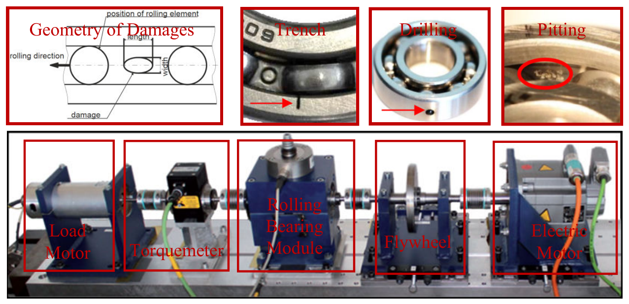
34] was developed by the Chair of Design and Drive Technology at Paderborn University (PU), Germany. The data were collected from a modular electromechanical drive system consisting of an induction motor, a flexible shaft, a rolling bearing module, and a controllable load unit, as illustrated in
Figure 3. The test rig was specifically designed to simulate realistic operating environments of industrial rotating machinery. During operation, both vibration and current signals were measured simultaneously under different rotational speeds and torque loads using high-precision sensors.
The dataset contains three bearing fault types. The test bearings used in the PU bearing dataset were FAG deep-groove ball bearings. Artificial defects were introduced on the inner race, outer race, and rolling elements using electrical discharge machining, with defect diameters of 0.1, 0.3, and 0.5 mm. Real degradation samples were obtained through long-term accelerated fatigue experiments until the occurrence of natural damage. The typical damage locations and corresponding examples are shown in
Figure 3. Each bearing condition was tested under multiple working scenarios, including rotational speeds of 900 rpm and 1500 rpm, and torque loads of 0.1 Nm, 0.7 Nm, and 1.3 Nm, yielding a comprehensive dataset that reflects representative operating conditions. The vibration signals were sampled at 64 kHz, with each record corresponding to approximately 4 s of measurement. The dataset includes both time-domain vibration signals and associated condition labels. This study exclusively employs vibration data and considers three fault types to assess the generalization performance of the proposed simulation-driven diagnosis framework.
4.1.2. Impulse Synthesis Results on the PU Bearing Dataset
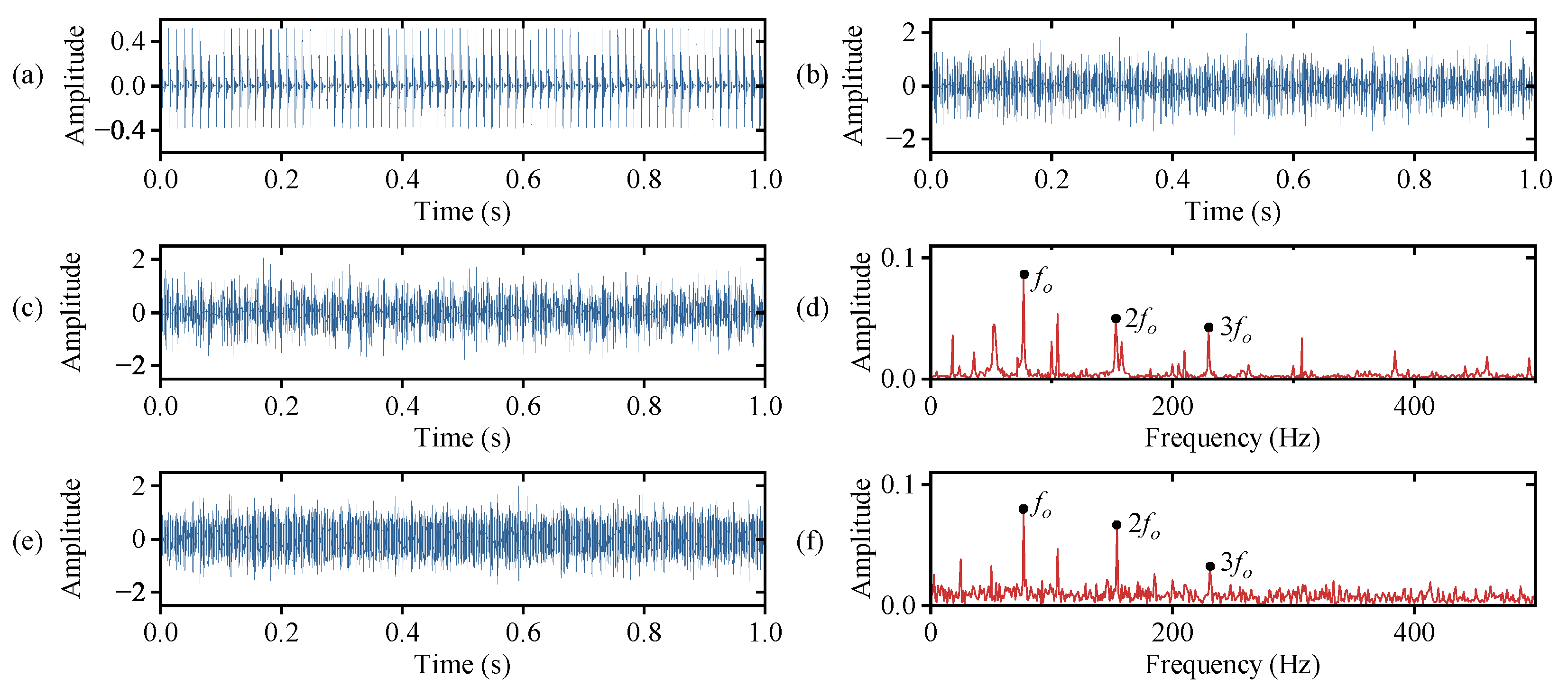
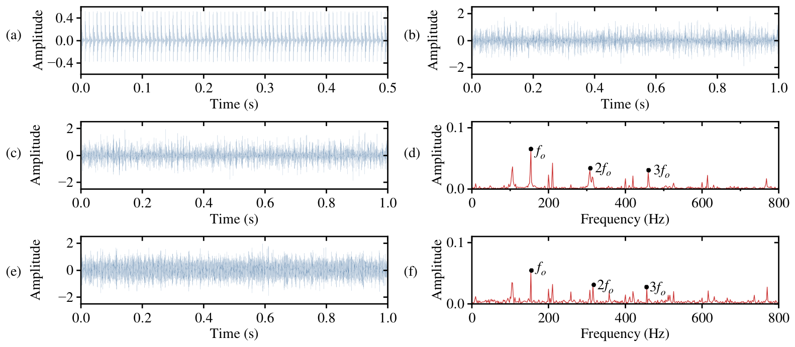
Figure 4 presents the synthesis and comparison of outer race fault signals used in this experiment. As shown in
Figure 4a, periodic fault impulses were generated according to the theoretical characteristic frequency of the outer race defect. The corresponding healthy bearing vibration signal measured under normal operation is shown in
Figure 4b. By superimposing the simulated impulses on the measured healthy signal, a mixed vibration signal with an outer race defect was obtained, as shown in
Figure 4c. The amplitude of the simulated impulses was carefully selected to be slightly higher than the normal vibration level, ensuring both physical realism and sufficient fault visibility.
The envelope spectrum of the synthesized fault signal is displayed in
Figure 4d. The dominant frequency components were well aligned with the theoretical fault characteristic frequency
and its harmonics, which confirmed the accuracy of the simulation procedure. For reference, the experimentally measured outer race fault signal from the PU dataset and its envelope spectrum are shown in
Figure 4e,f. Both spectra exhibit similar harmonic structures and fault-related frequency components, demonstrating that the synthesized data effectively emulated the essential modulation characteristics of real bearing faults. Minor discrepancies in amplitude and resonance bandwidth were attributed to stochastic excitation, load fluctuations, and nonlinear coupling in the experimental setup.
4.1.3. Diagnosis Results Under Fault-Free Conditions
In this subsection, the proposed simulation-driven diagnostic framework was evaluated using the PU bearing dataset under fault-free training conditions. The objective was to assess whether the proposed model, trained exclusively on healthy signals and synthesized pseudo-fault samples, could identify real bearing faults without using real fault samples during training. This setting reflected realistic industrial scenarios in which fault samples were limited or unavailable.
Considering the completeness of diagnostic classes and the representativeness of different speed-load combinations, four operating conditions were selected from the PU bearing dataset for evaluation: Condition 1, 900 rpm and 0.1 Nm; Condition 2, 900 rpm and 0.7 Nm; Condition 3, 1500 rpm and 0.1 Nm; and Condition 4, 1500 rpm and 0.7 Nm. These selected conditions covered different combinations of rotational speed and load, thereby enabling the evaluation of the proposed framework under varying working conditions.
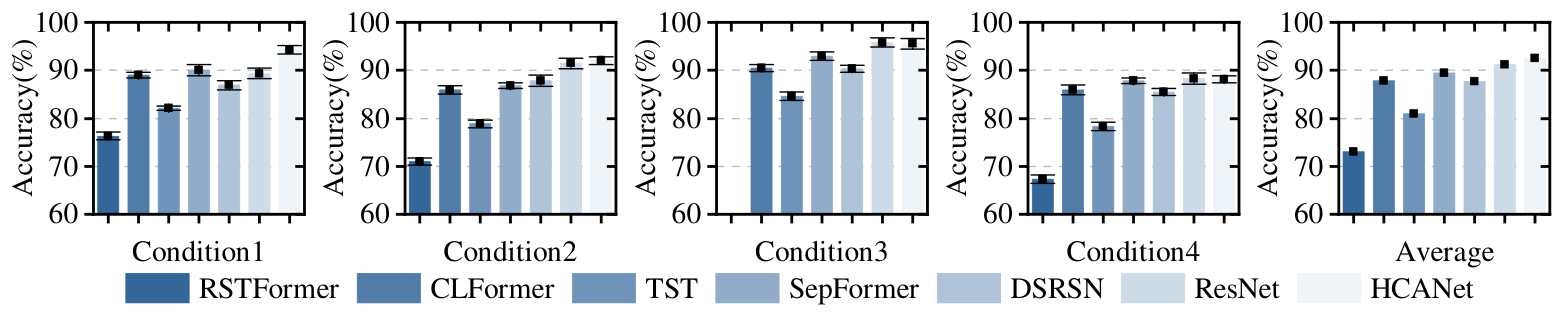
Figure 5 compares the diagnostic accuracy results of several representative deep-learning-based models across the four selected operating conditions in the PU dataset. As shown in
Figure 5, the proposed HCANet achieved the highest average accuracy and maintained competitive performance across all operating conditions. HCANet attained an average accuracy of 92.50%, exceeding ResNet by 1.27 percentage points and outperforming the transformer-based RSTFormer by 19.49 percentage points. This overall advantage indicated that the hierarchical convolutional attention architecture effectively enhanced both local feature extraction and long-range dependency modeling, thereby supporting robust generalization across different working conditions. In particular, the stable performance across varying load-speed combinations indicated the adaptability of the proposed framework to the distribution discrepancy between synthesized pseudo-fault training samples and real-fault testing samples.
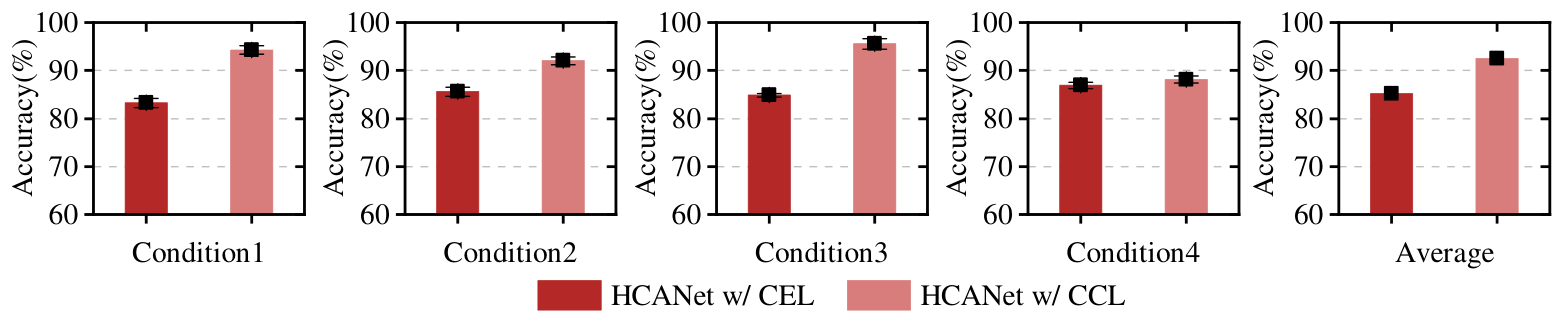
To further examine the contribution of the proposed Central Clustering Loss (CCL), an ablation study was conducted by replacing CCL with the conventional cross-entropy loss (CEL), while keeping the network architecture, input features, and training settings unchanged. As shown in
Figure 6, HCANet with CEL achieved an average accuracy of 85.15%, whereas HCANet with CCL achieved an average accuracy of 92.50%. Therefore, CCL improved the average diagnostic accuracy by 7.34 percentage points. This improvement indicated that, within the proposed framework, CCL was more effective than CEL in learning discriminative representations under fault-free training conditions.
The performance gain of CCL was attributed to its center-based metric-learning mechanism. By optimizing the cosine similarity between sample embeddings and their corresponding class centers, CCL encouraged samples from the same class to form more compact clusters while increasing inter-class separation in the embedding space. This property was particularly beneficial when the model was trained on synthesized pseudo-fault samples but tested on real fault samples, since a compact and well-separated embedding space helped improve the transferability of fault representations between pseudo-fault and real-fault distributions.
Overall, these results verified the effectiveness of the proposed simulation-driven framework in learning transferable fault representations from healthy signals augmented with synthesized pseudo-fault samples. The combination of hierarchical convolutional attention and CCL allowed HCANet to achieve high diagnostic accuracy and strong generalization capability even in the absence of real fault samples during training.
4.2. Experimental Study on the Drivetrain Simulator Bearing Dataset
4.2.1. Description of the Drivetrain Simulator Bearing Dataset
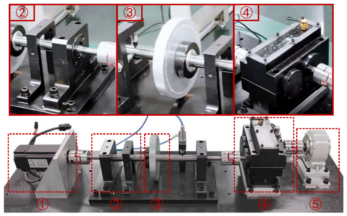
The drivetrain simulator bearing dataset was collected on a dedicated drivetrain test platform constructed for condition monitoring and fault analysis of high-speed train transmission systems. As shown in
Figure 7, the test rig consisted of five major components: (1) a three-phase induction motor used as the primary drive source, (2) a bearing housing for installing test bearings under different health conditions, (3) a flywheel assembly for introducing rotational inertia and stabilizing the drivetrain, (4) a dual-stage gearbox for torque transmission and speed regulation, and (5) a magnetic powder brake for applying variable mechanical loads. This modular configuration enabled the flexible emulation of diverse drivetrain operating conditions by independently adjusting the motor speed and brake torque.
To monitor the dynamic response of the bearing system, multi-modal sensing was employed. HDYD-232 piezoelectric accelerometers (Wuxi Houde Automation Meter Co., Ltd., Wuxi, China) were mounted on the bearing housing to collect tri-axial acceleration signals. All channels were recorded simultaneously at 100 kHz through a multi-channel data acquisition platform, which ensured fine temporal resolution and reliable synchronization across mechanical and electrical signals. This design allowed comprehensive analysis of vibration and current features under various bearing health states.
The dataset included several operating conditions determined by combinations of rotational speed and load. NSK deep-groove ball bearings were installed in the bearing housing to acquire signals under different health states. In particular, three speed settings, 1500, 2000, and 2500 rpm, together with two torque loads levels of 5 Nm, and 10 Nm, were considered. Under each condition, vibration and current measurements were acquired for four bearing health states: healthy, outer-race fault, inner-race fault, and rolling-element fault. This dataset provided a high-fidelity benchmark for evaluating intelligent diagnostic models under diverse and realistic operating conditions. In this study, the normal-state data were further used to synthesize pseudo-fault signals using the method introduced in
Section 3.1, enabling the evaluation of the proposed simulation-driven framework under fault-free training conditions.
4.2.2. Impulse Synthesis Results on the Drivetrain Simulator Dataset
Figure 8 illustrated the synthesis and comparison of outer race fault signals obtained from the drivetrain simulator bearing dataset. As shown in
Figure 8a, the periodic fault impulses were generated according to the theoretical fault characteristic frequency of the outer race defect. These impulses reproduced the repetitive impact excitations caused by rolling elements passing over localized damage. The corresponding vibration signal measured under normal operation was presented in
Figure 8b, representing the baseline healthy state of the drivetrain system. By superimposing the simulated periodic impulses onto the healthy signal, a synthesized vibration signal exhibiting an outer race fault pattern was produced, as shown in
Figure 8c. The amplitude and decay rate of the simulated impulses were selected to approximate the dynamic response characteristics of real bearing faults, ensuring both physical realism and diagnostic interpretability. The envelope spectrum of the synthesized signal was shown in
Figure 8d, where distinct peaks corresponding to the fundamental fault characteristic frequency
and its harmonics (
,
) were observed, confirming that the synthesized data effectively captured the modulation features associated with localized defects.
For validation, the experimentally measured outer race fault signal collected from the drivetrain simulator dataset and its corresponding envelope spectrum were depicted in
Figure 8e,f, respectively. Both the synthesized and real signals shared similar frequency-domain structures, particularly in the appearance of strong spectral components at integer multiples of
. This consistency demonstrated that the simulation-driven approach accurately reproduced the essential fault-related dynamics observed in real measurements. Minor discrepancies in amplitude and resonance bandwidth arose from practical nonlinearities, sensor placement variations, and load-induced stochastic disturbances in the test rig.
4.2.3. Fault Diagnosis Results on the Drivetrain Simulator Bearing Dataset
To comprehensively evaluate the generalization capability of the proposed simulation-driven diagnostic framework, experiments were conducted using the drivetrain simulator bearing dataset under fault-free training conditions. In this scenario, the model was trained exclusively on healthy vibration signals and synthesized pseudo-fault samples, while real fault samples were used only for testing. This design was intended to emulate realistic situations in which fault samples are scarce or unavailable during system commissioning and early operation, thereby assessing the ability of the model to generalize from synthesized pseudo-fault samples to real fault signals.
Considering the completeness of diagnostic classes and the representativeness of different speed-load combinations, five operating conditions were selected from the drivetrain simulator bearing dataset for evaluation: Condition 1, 1500 rpm and 5 Nm; Condition 2, 1500 rpm and 10 Nm; Condition 3, 2000 rpm and 5 Nm; Condition 4, 2500 rpm and 5 Nm; and Condition 5, 2500 rpm and 10 Nm. These selected conditions covered all three rotational speed levels and both load levels, including low-speed low-load, low-speed high-load, high-speed low-load, and high-speed high-load scenarios.
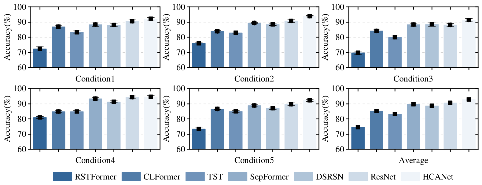
Figure 9 illustrates the diagnostic accuracies of various representative models under the five selected operating conditions. Among all compared methods, the proposed HCANet achieved the best performance across all five operating conditions. Specifically, HCANet attained an average accuracy of 92.84%, exceeding ResNet by 2.15 percentage points. Compared with Transformer-based baselines such as CLFormer and SepFormer, HCANet improved the average accuracy by 7.55 and 3.24 percentage points, respectively. Under Condition 1, HCANet still maintained an accuracy of 92.15%, indicating its robustness under relatively challenging operating conditions. Across Conditions 3–5, HCANet also maintained stable diagnostic performance, with accuracies of 91.33%, 94.62%, and 92.27%, respectively, all remaining above 90%. These results indicated that the hierarchical grouped convolution and multi-head attention mechanisms allowed HCANet to capture cross-band correlations and long-range dependencies effectively, thereby enhancing the discriminability of fault-related features.
To further examine the contribution of the proposed Central Clustering Loss (CCL),
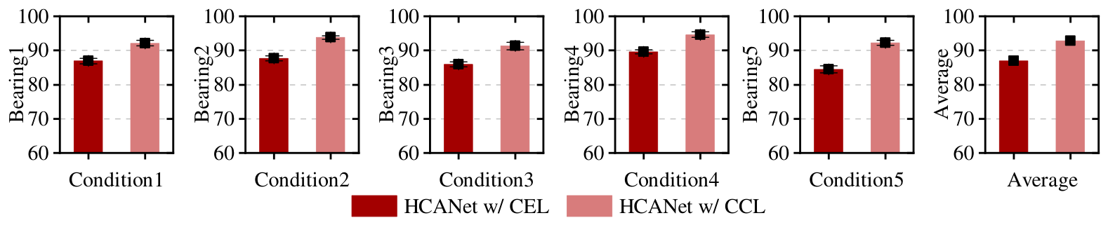
Figure 10 compares the diagnostic accuracies of two HCANet variants trained with the conventional cross-entropy loss (CEL) and CCL, respectively, while keeping the network architecture, input features, and training settings unchanged. As shown in
Figure 10, HCANet with CEL achieved an average accuracy of 86.91%, whereas HCANet with CCL achieved an average accuracy of 92.84%. Therefore, CCL improved the average diagnostic accuracy by 5.92 percentage points. The performance improvement was observed across all operating conditions, demonstrating that CCL provided a consistent enhancement over CEL across the tested operating conditions within the proposed framework. The advantage of CCL was attributed to its center-based metric-learning mechanism. By optimizing cosine similarities between sample embeddings and their corresponding class centers, CCL encouraged intra-class compactness while increasing inter-class separation in the embedding space. This was particularly beneficial under fault-free training conditions, where the model had to learn discriminative representations from synthesized pseudo-fault samples and then generalize to real fault signals. Consequently, the learned representations became more robust to the distribution discrepancy between pseudo-fault training samples and real-fault testing samples.
Overall, the experimental results demonstrated that the combination of hierarchical convolutional attention and CCL enhanced both representational robustness and discriminative capability. The proposed framework achieved accurate fault identification under fault-free training conditions, thereby improving the transferability of learned fault representations from synthesized pseudo-fault data to real fault data.
4.3. Ablation Results of Different WPD Decomposition Levels
The decomposition level of WPD directly affects the time–frequency resolution, feature dimensionality, and subsequent diagnostic performance. To justify the selection of two-level WPD in the proposed framework, an ablation study was conducted on the PU bearing dataset by varying the WPD decomposition level from one to four. During this comparison, the network architecture, loss function, training protocol, and testing conditions were kept unchanged, and only the WPD decomposition level was varied.
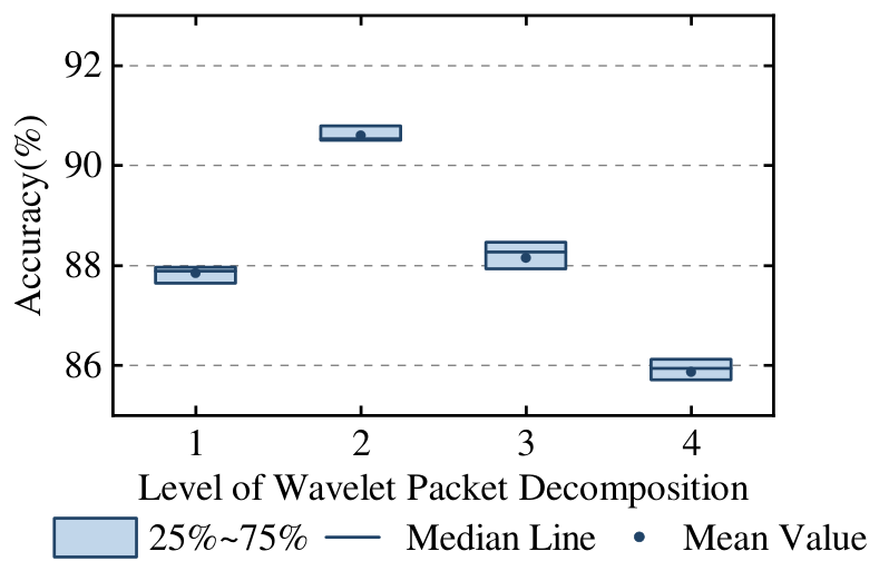
Figure 11 shows the diagnostic accuracy distributions under different WPD decomposition levels. The mean accuracies obtained with one-level, two-level, three-level, and four-level WPD were 87.90%, 90.61%, 88.28%, and 85.94%, respectively. Among them, two-level WPD achieved the highest mean diagnostic accuracy, improving the accuracy by 2.71, 2.33, and 4.66 percentage points compared with one-level, three-level, and four-level WPD, respectively. In addition, the accuracy distribution of two-level WPD was relatively compact, indicating stable diagnostic performance across repeated experiments.
The performance advantage of two-level WPD was mainly attributed to the trade-off between frequency localization and feature compactness. For an L-level WPD, the signal is divided into sub-bands. One-level WPD produced only two broad sub-bands, which may have been insufficient to separate fault-related resonance components from background vibration components. In contrast, higher-level decomposition provided finer frequency partitioning, but it also increased the number of sub-bands and may have split fault-related resonance and modulation information into multiple narrow frequency regions. This could have led to fragmented feature representations and increased the complexity of subsequent feature learning. Therefore, two-level WPD provided a more suitable balance between time–frequency resolution, feature compactness, and diagnostic performance in the proposed framework.
5. Conclusions
This study proposed a simulation-driven framework for bearing fault diagnosis under fault-free training conditions. To address the scarcity of real fault data, pseudo-fault signals were synthesized by superimposing periodic impulse–resonance responses governed by theoretical bearing fault characteristic frequencies onto healthy vibration signals. Wavelet packet decomposition and envelope spectrum analysis were employed to extract fault-sensitive time–frequency features. A Hierarchical Convolutional Attention Network was developed to capture local sub-band features and global dependency representations through grouped convolutions and multi-head attention mechanisms. A Central Clustering Loss was further introduced to enhance feature discriminability by promoting intra-class compactness and inter-class separation in the embedding space. Experiments on the Paderborn University and drivetrain simulator bearing datasets showed that the proposed method achieved high diagnostic accuracy without using real fault samples during training. Overall, the proposed framework provided a feasible solution for zero-real-fault-data diagnosis, enabling reliable fault identification and extending the applicability of intelligent monitoring systems in practical condition monitoring scenarios. Scientifically, this study provided a mechanism-guided framework for bearing fault diagnosis without real fault samples during training. By integrating fault-mechanism modeling, time–frequency analysis, and deep representation learning, the method helped bridge healthy vibration data and real fault identification. Socially and engineering-wise, it has the potential to reduce destructive fault induction experiments, lower data acquisition costs, and support safer condition monitoring of industrial rotating machinery. Although the proposed framework achieved promising performance under fault-free training conditions, its robustness to strong noise interference was not fully investigated. Future work will focus on improving the pseudo-fault synthesis strategy and enhancing the noise robustness of the diagnostic model. More realistic pseudo-fault samples may be generated by incorporating three-dimensional dynamic simulation models, and noise-robust neural network architectures will be further explored to improve the applicability of the proposed framework in harsh industrial environments.