Fast Driving Cycle Efficiency Optimization of Interior Permanent Magnet Synchronous Machines Considering PWM-Induced Harmonic Losses

Abstract

A multi-objective optimization framework is developed in this work to improve the driving cycle efficiency of IPMSMs, into which a fast-computational approach for PWM-induced harmonic losses is embedded. At a set of characteristic operating points, iron losses are first evaluated under sinusoidal current source (SCS) excitation using Computationally Efficient Finite Element Analysis (CE-FEA), while a Time-Stepping Finite Element Analysis (TS-FEA) spanning one quarter of the electrical period provides the copper losses. For scenarios where the machine is driven by a pulse-width modulation (PWM) voltage source inverter, the harmonic losses arising from modulation are quickly assessed through a small-signal time-harmonic finite element method (THFEA)-based model. The resulting optimization procedure seeks a trade-off between two conflicting goals: minimizing overall losses and reducing material cost. Given an equal cost level, incorporating PWM-related harmonic losses into the design loop cuts down the total loss by 3.11% relative to a baseline that only considers SCS-supply losses. The extra computational burden amounts to 17 h, representing a time rise of roughly 22.65%.

1. Introduction

Owing to advantages such as high specific power, superior energy conversion efficiency, responsive dynamic behavior, and a space-saving layout, interior permanent magnet synchronous machines (IPMSMs) have become the dominant choice of traction motors in battery electric vehicles. Accordingly, enhancing their efficiency [1], curbing their loss generation, directly contributes to extending the driving distance per charge. Moreover, loss mitigation also eases thermal management requirements and reduces associated cooling expenses.

Many papers have been published regarding the optimization of the efficiency of IPMSMs for EVs [2,3,4,5,6,7,8,9,10]. Unlike industrial motors that operate under fixed conditions for extended periods, IPMSMs for EVs operate under varying conditions for a long time. Therefore, when assessing their efficiency, it is necessary to consider the driving conditions of EVs, which increases the difficulty of rapid and accurate calculation. The state-of-the-art method for solving this problem is to choose representative points (RPs) based on the drive cycle of EVs for computing the weighted average loss, and these RPs can be obtained from the geometric or energy center of gravity [2,3], k-means clustering [5,6], fuzzy C-means clustering [7], and X-means clustering methods [8]. Another useful technique for speeding up the efficiency calculation is computationally efficient finite element analysis (CE-FEA), with which the electromagnetic characteristics of IPMSMs with distributed windings under sinusoidal current source (SCS) supplies can be obtained using only 1/6 of the electrical period of time-stepping finite element analysis (TSFEA).

A key limitation of the efficiency analysis in reference [10,11,12] lies in its omission of PWM-induced harmonic effects. Under PWM voltage source inverter operation—particularly common in EV propulsion systems—these harmonic losses are far from negligible. For example, ref. [13] reports that at low-speed, light-load conditions, such losses can exceed 40% of the total machine loss, which is precisely the operating region where urban-driving EVs predominantly reside [14,15,16,17].

In [18], PWM-induced harmonic losses were taken into account during the optimization process of IPMSMs. By optimizing the stator and rotor structures, PWM harmonic losses were reduced by 20%, resulting in an improvement of 0.9 percentage points in motor efficiency under low-speed and light-load conditions. It should be noted that both time measurements were obtained using the same computing platform. This significant time increase occurs because [18] employed time-stepping finite element analysis (TSFEA) using the PWM transient voltage waveform as input to calculate PWM-induced harmonic losses [19]. This method requires extremely fine time steps to resolve high-frequency harmonics, leading to excessively long calculation times.

A computationally efficient approach for estimating PWM-induced harmonic losses in IPMSMs was recently proposed, relying on the small-signal time-harmonic finite element formulation (THFEA) [19,20,21,22,23,24]. Within this framework, the mapping from injected high-frequency harmonic voltages (HFHVs) to the resulting losses in permanent magnets, ferromagnetic cores [19], and copper windings can be explicitly derived. Using this scheme, one can directly feed the voltage spectral content of PWM waveforms into the model to obtain harmonic losses across various operating states without time-consuming transient simulations. The method reportedly achieves accuracy comparable to conventional TSFEA that employs full PWM transient voltage waveforms [22], and its validity has been further confirmed by experimental measurements [17].

In [25], the fast driving-cycle efficiency optimization of an IPMSM with hairpin windings considering PWM-induced harmonic losses is achieved by incorporating the fast monic loss calculation method based on the small-signal THFEA into the multi-objective optimization process. However, in [25], the hysteresis loss under SCS supply is estimated from eddy current loss calculated with the dynamic iron loss model [26] for saving computational time, which sacrifices the calculation accuracy of hysteresis loss. In addition, the AC copper loss under SCS supply in [25] is estimated with analytical methods, which also introduces errors. This paper further improves upon the work presented in [25]. The iron loss under SCS supply is computed with the CE-FEA and the AC copper loss is computed using the TSFEA with the minimum number of time steps, aiming to enhance the speed of optimization calculations as much as possible without sacrificing calculation accuracy.

In Section 2, nine RPs and their weight factors for the prototype IPMSM are calculated based on the driving cycle using both analytical methods and k-means clustering methods. In Section 3, the calculation methods for the maximum torque-speed curve, iron loss and AC copper loss under SCS supply, as well as PWM-induced harmonic losses, are detailed. In Section 4, a multi-objective optimization process for IPMSMs considering PWM harmonic losses is presented. The Pareto frontiers and optimized structures are compared when PWM-induced harmonic losses are considered versus when they are neglected. Conclusions are drawn in Section 5.

2. Driving Cycle Analysis and Prototype Parameters

2.1. Vehicle Parameters and Driving Cycle Analysis

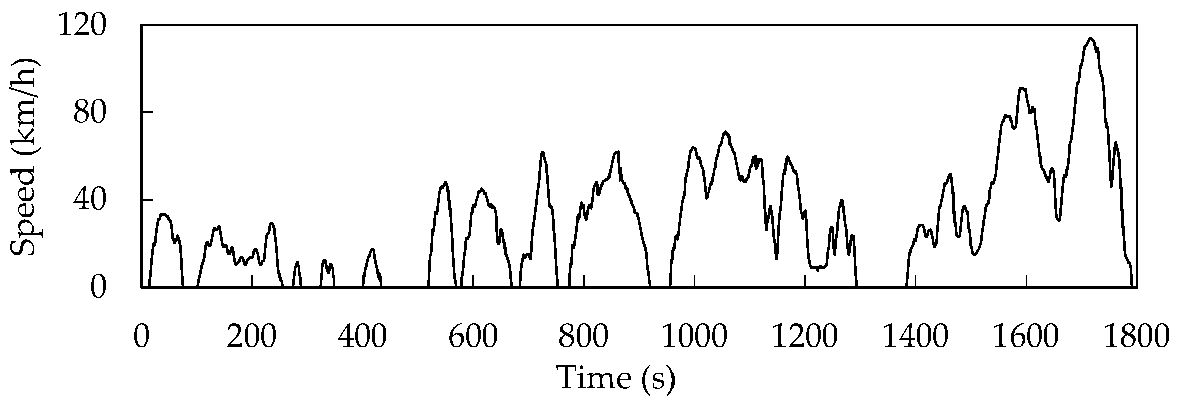
Two official driving schedules are specified for light-duty automobiles in China: the China light-duty vehicle test cycle for passenger cars (CLTC-P) and a distinct cycle for commercial vehicles. In this work, the CLTC-P serves as the basis for all subsequent calculations, and its speed evolution as a function of time is visualized in Figure 1.

The output torque required by the IPMSM can be calculated based on the vehicle’s parameters and driving conditions [27], which is shown as:

$$\left\{\begin{array}{l}{F}_{drive}=F_f+F_w+F_i+F_j\\ T={\displaystyle \frac{F_{drive}r}{k\eta }}\end{array}\right.$$

(1)

$$\left\{\begin{array}{l}{F}_f=\mu mg\cos \theta \\ F_w={\displaystyle \frac{1}{2}}\rho A{C}_D{v}^2\\ F_j=(m+{\displaystyle \frac{\delta k^2\eta }{r^2}})\cdot a\\ F_i=mg\sin \theta \end{array}\right.$$

(2)

where F_drive is the total driving force acting on the vehicle, and T denotes the mechanical torque produced by the motor. The symbols F_f, F_w, F_i, and F_j represent the rolling, aerodynamic, grade, and inertia resistance forces, respectively, while θ corresponds to the road gradient. All other relevant parameters are listed in

Table 1. Vehicle parameters.

Symbol	Vehicle Parameters	Unit	Value
m	Vehicle weight	kg	2050
r	Tire radius	m	0.25
g	Acceleration of gravity	m/s2	9.8
μ	Coefficient of rolling friction	-	0.02
ρ	Air density	kg/m3	1.25
A	Frontal area	m2	2.2
CD	Coefficient of aerodynamic drag	-	0.42
δ	Inertia coefficient	-	0.0025
η	Gear efficiency	-	0.90
k	Gear ratio	-	9.18

.

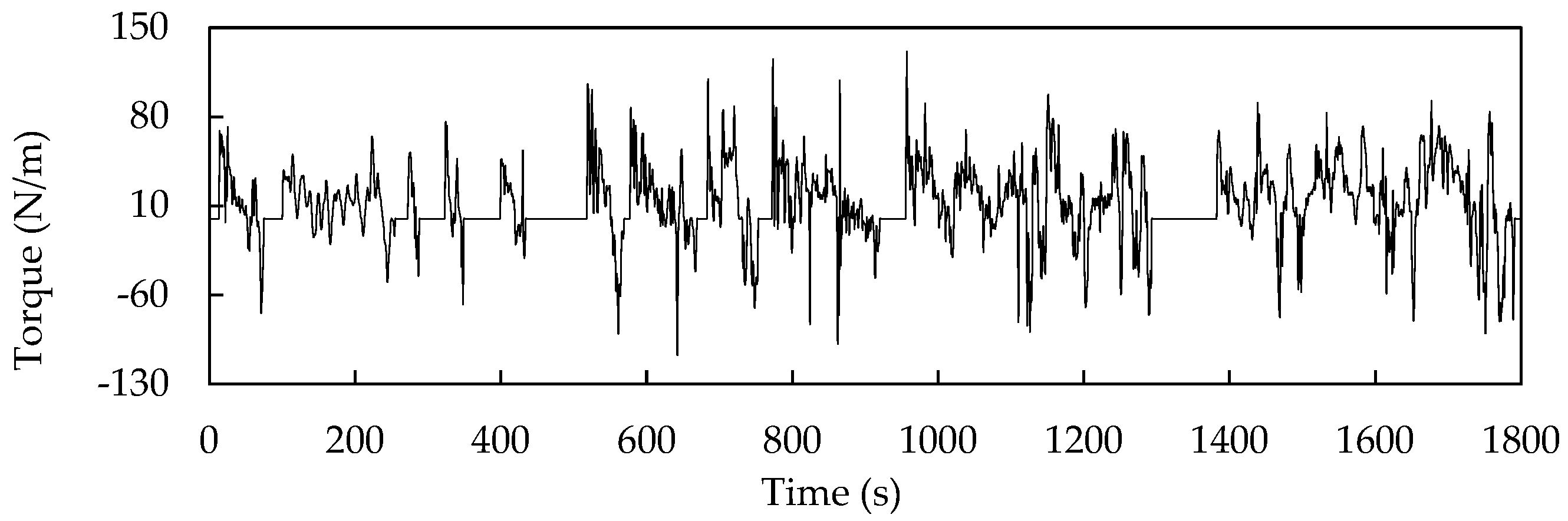
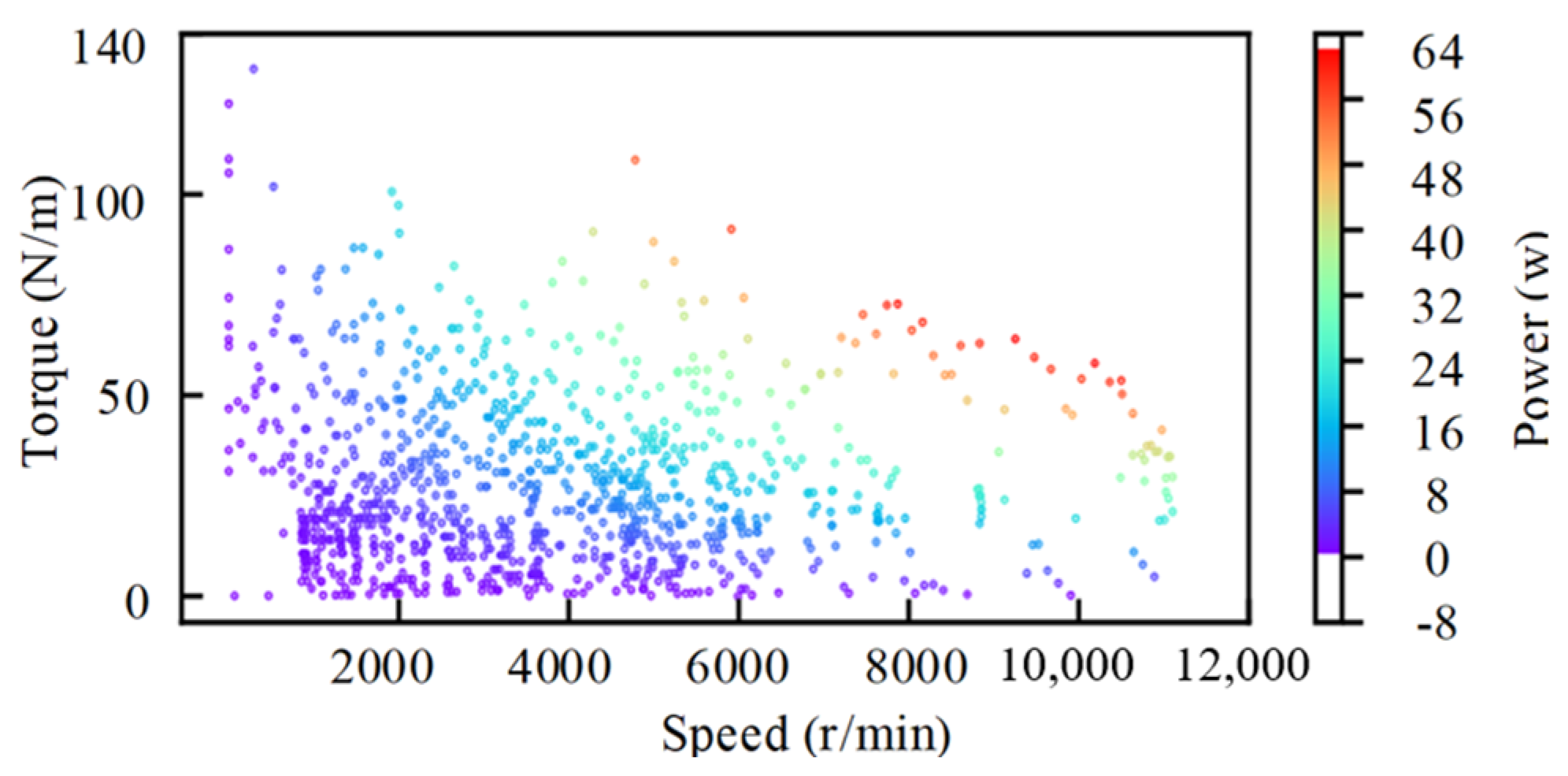
Figure 2 shows the time-dependent torque profile of the IPMSM obtained from these dynamic relations. To reduce computational effort, the motor is assumed to generate zero torque during standstill or deceleration events. After post-processing the simulated data, Figure 3 depicts how the motor’s output torque, speed, and power are distributed relative to one another.

2.2. k-Means Cluster

Since a full driving cycle contains numerous operating points, performing FEA-based loss calculations for every point would be computationally prohibitive, especially when multiple motor designs must be evaluated. To reduce this burden, the k-means clustering method [6] is adopted to extract RPs, based on the observation that losses and efficiencies remain nearly constant across neighboring operating conditions. The overall cycle performance is then assessed using these RPs.

In the k-means algorithm, an initial set of k cluster centers is first chosen. Each data point is then assigned to the nearest center, forming clusters. Subsequently, each cluster center is updated to the mean of its assigned points. This assign–update iteration continues until the centers no longer change. The detailed mathematical expressions are given below.

$$S_i^{(t)}=\left\{x_p\left|{‖x_p-m_i^{(t)}‖}^2\le {‖x_p-m_j^{(t)}‖}^2\forall j,1\le j\le k\right.\right\}$$

(3)

$$m_i^{(t+1)}={\displaystyle \frac{1}{\left|S_i^{(t)}\right|}}{\displaystyle \sum _{x_j\in S_i^{(t)}}{x}_j}$$

(4)

where S_i^(t) represents the i-th cluster formed during the t-th iteration, while x_p denotes an individual data sample assigned to that cluster. The centroids of the i-th and j-th clusters are denoted by m_i and m_j, respectively.

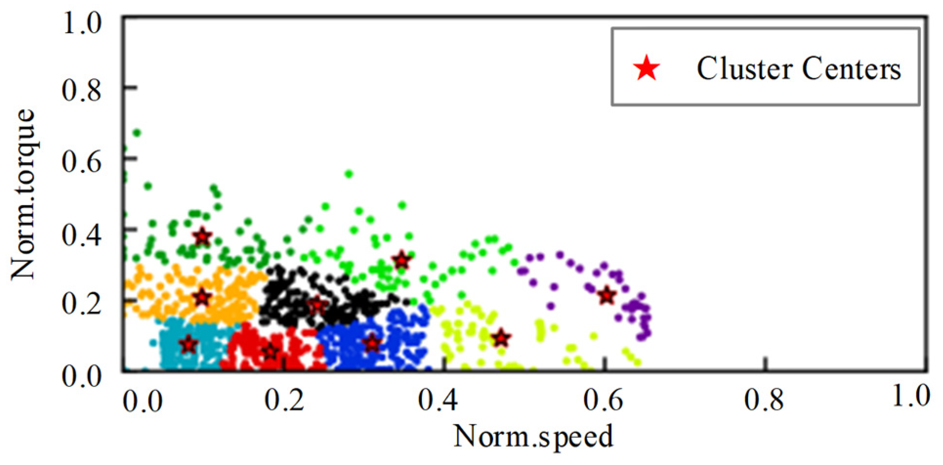
Based on design specifications, the IPMSM used in this study has a maximum torque rating of 195 Nm and a maximum rotational speed of 17,000 r/min. Prior to clustering, min–max normalization is applied to the dataset to scale all features appropriately. The k-means algorithm is subsequently performed on the CLTC-P driving cycle data, from which 9 RPs are extracted together with their respective occurrence frequencies. The resulting cluster distribution is visualized in Figure 4, and a detailed breakdown of the nine selected RPs is provided in

Table 2. Nine Cyclic RPs.

RP Number	Speed (r/min)	Torque (N/m)	Weight Factors, wi
1	1422	13.937	0.18164
2	1650	39.312	0.12754
3	1662	73.243	0.06473
4	3185	11.373	0.14106
5	4170	37.067	0.14783
6	5285	15.145	0.17488
7	5913	61.508	0.05700
8	8004	18.137	0.06957
9	10,241	41.674	0.03575

.

Consistent with observations reported in [3], the CLTC-P cycle exhibits the highest probability density in the low-speed, low-torque operating region for the IPMSM.

2.3. Machine Parameters

The baseline machine selected for this driving-cycle-based efficiency optimization study is an IPMSM featuring a 48-slot, 8-pole rotor configuration with a double-layer permanent magnet arrangement.

Table 3. Parameters of the prototype IPMSM.

Parameters	Value
Stator outer diameter (mm)	220
Rotor inner diameter (mm)	60
Air gap length (mm)	1.22
PM remanence	1.26
Relative permeability of PM	1.052
PM conductivity (S/m)	625,000
Number of poles	8
Maximum phase current, Im (A)	295 (RMS value)
DC bus voltage (V)	450
Switching frequency (Hz)	8000
Number of parallel branches	2
Maximum speed (r/min)	17,000
End leakage inductance (H)	7.34 × 105
Eddy current loss coefficient of ESSs (W/m3/Hz2/T2)	0.329
Hysteresis loss coefficient of ESSs (W/m3/Hz2/T2)	149.55
Thickness of one ESS (mm)	0.3
Conductivity of ESSs (S/m)	2.84 × 106
Maximum torque (Nm)	>195
Maximum power at 17,000 r/min (kW)	>120
Maximum torque at 17,000 r/min (Nm)	>67.407

lists the fixed design parameters along with the relevant constraints applied during the optimization.

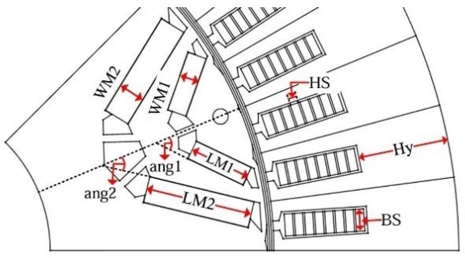
Figure 5 illustrates the geometric design variables subject to optimization for this prototype IPMSM, and their allowable variation intervals are summarized in

Table 4. Optimization variables and variation ranges.

Variables	Unit	Range
Small PM pole arc, ang1		36–55
Large PM pole arc, ang2		30–45
Copper conductor width, BS	mm	3–5.3
Copper conductor thickness, HS	mm	1.2–1.9
Yoke length, Hy	mm	10–20
Small PM width, LM1	mm	9–14
Small PM thickness, WM1	mm	2–5
Large PM width, LM2	mm	18–24
Large PM thickness, WM2	mm	3.5–7.8
Axial length, L_axis	mm	70–90

. These upper and lower bounds are established according to real-world engineering practices, with the initial dimensions serving as the reference around which appropriate limits are defined. Any geometric parameters that exhibit mutual incompatibility or redundancy are excluded from the optimization routine. It should be noted that several key dimensions, namely the airgap length, the rotor inner diameter, and the stator outer diameter—as reported in Table 3—are held constant throughout the entire optimization process.

3. Characteristics Calculation of IPMSM

3.1. Torque-Speed Envelop Calculation

To calculate the maximum output torques of the IPMSM at different speeds, as well as the d- and q-axis currents (i_d and i_q) at various rotational speeds and torques, it is first necessary to obtain the relationships between the torque, d- and q-axis flux linkages, and i_d and i_q. However, magnetic saturation, cross-coupling effects, and spatial harmonics all affect the relationships between the torque, flux linkages, and currents [28]. Hence, parametric sweep FEA under the excitations of different i_d and i_q at different rotor positions (θ_e) must be conducted to accurately calculate these relationships, which is rather time-consuming, especially in the optimal design process. To obtain the minimum number of FEA steps required to accurately calculate the maximum torques at different speeds, the maximum torques at 1000 r/min and 17,000 r/min of three IPMSMs with different geometry parameters, as shown in

Table 5. Geometry parameters of three IPMSMs.

Variables	Unit	Structure 1	Structure 2	Structure 3
ang1		52.58	37.58	48.48
ang2		42.08	33.16	37.08
BS	mm	3.39	4.81	5.0661
HS	mm	1.34	1.63	1.63
Hy	mm	11.22	10.32	20.7675
LM1	mm	11.25	12.76	12.2776
WM1	mm	4.43	3.69	3.7944
LM2	mm	23.48	23.90	21.21
WM2	mm	4.07	4.57	5.151
L_axis	mm	85.52	78.82	80

, are computed based on the flux and torque maps obtained with different FEA results.

The maximum torque per ampere (MTPA) and maximum torque per voltage (MTPV) strategies are used for computing the maximum torque values [29,30]. When conducting the parametric sweep FEA, the chosen i_q distribute uniformly between 0 and $\sqrt{2}{I}_m$, while i_d increases from $-\sqrt{2}{I}_m$ to 0. Because the variations in torque and flux linkages with rotor positions have a period of 60 electrical degrees [28], conducting FEA at different rotor positions within a 1/6 electrical period is enough for computing the average values of torque and flux linkages.

Table 6. Maximum torques at different speeds calculated with different parametric sweep FEA results.

Case	Structure 1 (Nm)		Structure 2 (Nm)		Structure 3 (Nm)
	1000 r/min	17,000 r/min	1000 r/min	17,000 r/min	1000 r/min	17,000 r/min
10id × 10iq × 20θe	249.95	63.75	217.2	66.48	205.79	69.04
5id × 5iq × 20θe	250.87	63.87	217.99	66.90	206.06	69.25
5id × 5iq × 5θe	250.79	63.68	217.93	66.77	206.05	69.25
5id × 5iq × 4θe	251.54	63.98	217.64	66.38	204.64	68.44
5id × 5iq × 3θe	250.74	63.89	218.16	67.04	206.10	68.94
5id × 5iq × 2θe	231.36	53.02	199.32	55.31	203.37	64.60
4id × 4iq × 5θe	249.73	66.16	217.03	68.94	205.75	70.61
3id × 3iq × 5θe	247.93	69.48	216.39	71.54	203.52	73.36
2id × 2iq × 2θe	219.94	71.74	191.25	71.36	191.81	73.97

compares the maximum torques of the three structures at different speeds calculated from different parametric FEA results. The number of i_d and i_q must not be less than 5 to ensure the accuracy of the calculated torque at the maximum speed. The rotor position number should not be less than 3 to ensure the calculation accuracy of the torques, and the errors obtained with four rotor positions may be larger than those obtained with three rotor positions. Hence, in the following optimization process, the number of i_d and i_q is set to 5, and the rotor position number in the 1/6 electrical period is set to be 3 for computing the torque and flux linkage maps.

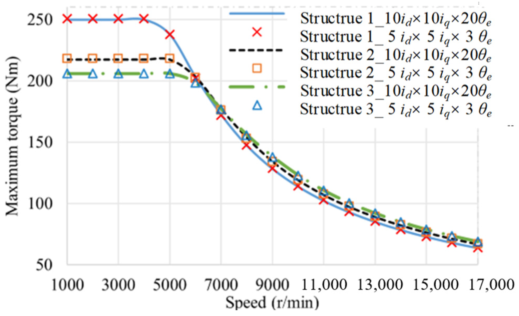
Figure 6 compares the maximum torque-speed plots calculated with different parametric sweep FEA results for the two structures. Using 5i_d × 5i_q × 5θ_e for conducting the parametric sweep FEA is enough for accurately calculating the maximum torque.

3.2. AC Copper Loss Calculation with TSFEA

With the torque and flux linkage maps obtained from the parametric sweep FEA, the i_d and i_q at nine RPs shown in Table 2 can be computed. Because the maximum torques at 17,000 r/min of structure 1 and 2 do not satisfy the requirement in Table 3, structure 3, shown in Table 5, is chosen as an example for illustrating the AC copper loss calculation method. The i_d and i_q at nine RPs for structure 3 are shown in

Table 7. Comparison of average AC copper losses calculated with different Δθ_e and different ranges for Structure 3.

RP Number	id (A)	iq (A)	Average AC Copper Loss (W)
			101–120 Step (Δθe = 3°)	11–15 Step (Δθe = 6°)
1	−2.38	31.62	13.00	12.89
2	−22.14	83.74	78.66	78.55
3	−63.33	140.25	238.55	238.58
4	−1.42	25.87	21.26	20.70
5	−19.65	79.63	100.93	99.84
6	−2.91	34.31	49.59	48.04
7	−47.77	121.57	264.79	262.22
8	−4.42	40.90	96.44	93.01
9	−105.74	67.52	267.55	266.53

.

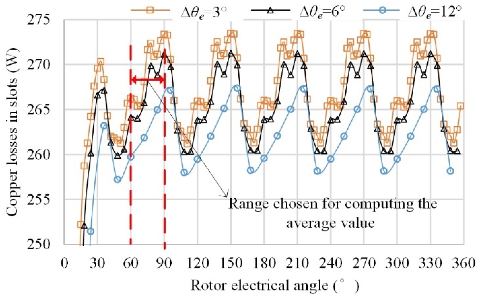
Then, the losses at the nine RPs need to be calculated for conducting the efficiency optimization. In [25], the AC copper losses are computed with the sum of those calculated with analytical equations and those at no-load conditions, which sacrifices the accuracy to avoid TSFEA at different conditions. In this paper, to improve calculation accuracy, TSFEA is directly used for calculating the AC copper losses in slots. Decreasing the time step of TSFEA will increase the calculation accuracy of AC copper losses, but it will also increase the calculation time. Hence, suitable steps need to be determined to balance the accuracy and the calculation time. Figure 7 shows the copper losses calculated with different time steps at the ninth RP in Table 2, where Δθ_e represents the electrical angle at which the rotor rotates each time step. In the first 1/6 of electrical period, the copper loss increases from 0 to reach the steady value, which means the results at the first 1/6 electrical period cannot be used to calculate the average AC copper loss. In addition, the calculated AC copper loss decreases with the increase in Δθ_e. Based on the above analysis, Δθ_e is chosen as 6° and 15 steps of TSFEA are conducted for computing AC copper losses. Hence, the average AC copper loss will be calculated by averaging the calculation results obtained from step 11 to step 15 in the following optimization procedure.

For further testifying the accuracy of the proposed method for calculating AC copper losses, the losses calculated with the proposed method at the nine RPs are compared with the average value for the last 1/6 electrical period when Δθ_e is 3°. They agree well with each other, as shown in Table 7. In addition, the PM loss under SCS supply, P_PM^scs, can be computed simultaneously when computing copper losses. Because the PM loss under SCS supply is much smaller [17], they are not shown here.

3.3. Iron Loss Calculation with CE-FEA

When calculating iron losses with the dynamic iron loss model [26], one electrical period of TSFEA needs to be conducted for accurately calculating hysteresis losses, which is rather time-consuming for the optimization procedure. In [27], it is proposed to use eddy current loss to estimate hysteresis loss for saving computational time when the dynamic iron loss model is used, which satisfies the accuracy. Alternatively, CE-EFA employs the symmetry of electrical machine using the flux density waveforms obtained with the minimum steps of TSFEA to reconstruct the flux density waveforms over one electrical period. For the IPMSM with distributed windings, TSFEA with a 1/6 conducting period was enough for obtaining the flux density waveform in each element over the entire period. Then, iron losses can be computed with both the dynamic model [28] or the frequency-domain model.

For computing AC copper losses, TSFEA in the first 1/4 electrical period has been conducted. Using the flux density waveform of each element in ESSs in the first 1/6 electrical period, CE-FEA can be directly employed for computing iron losses at the nine RPs. In this paper, the frequency-domain iron loss model [15] is combined with CE-FEA for computing iron losses. The calculation results are compared with those obtained from one electrical period TSFEA using the dynamic iron loss model [26], as shown in

Table 8. Comparison of iron losses calculated with different methods for Structure 3 at 9 RPs.

RP Number	Speed (r/min)	Torque (N/m)	Hysteresis Loss, Pihyssscs (W)		Eddy Current Loss, Piedscs (W)
			TSFEA	CEFEA	TSFEA	CEFEA
1	1422	13.937	26.68	26.89	7.40	7.42
2	1650	39.312	33.90	34.07	10.41	10.44
3	1662	73.243	39.44	40.01	12.83	12.89
4	3185	11.373	59.22	59.93	37.09	37.21
5	4170	37.067	85.12	85.36	65.90	66.12
6	5285	15.145	99.01	100.24	102.23	102.63
7	5913	61.508	133.71	135.67	152.98	153.55
8	8004	18.137	152.68	152.96	234.83	235.57
9	10,241	41.674	149.28	151.24	335.73	337.02

. The iron losses calculated with the two methods agree well, demonstrating the possibility of using CE-FEA to compute the iron loss under SCS supply to save computation time.

Finally, the total loss under SCS supply can be calculated as:

$$P_{scs}=P_{cs}^{scs}+P_{ce}^{scs}+P_{PM}^{scs}+P_{ied}^{scs}+P_{ihys}^{scs}$$

(5)

where P_cs^scs is the copper loss in slots, while P_ce^scs is the copper loss of end windings, which is simply computed with currents and the DC resistance of end windings [25].

3.4. Fast Calculation of PWM-Induced Harmonic Losses

This paper employs the small-signal THFEA method in [17] to rapidly calculate the PWM-induced harmonic losses using PWM voltage spectra as input. The relationships between harmonic losses in different parts and harmonic voltages can be expressed as:

$$\left\{\begin{array}{l}{P}_{st}^E\left(f_h\right)=U_{\alpha h}^2\cdot {\chi }_d^s\left(f_h\right)+U_{\beta h}^2\cdot {\chi }_q^s\left(f_h\right)\\ P_{st}^H\left(f_h\right)=U_{\alpha h}^2\cdot {\eta }_d^s\left(f_h\right)+U_{\beta h}^2\cdot {\eta }_q^s\left(f_h\right)\\ P_{rot}^E\left(f_h\right)=U_{dh}^2\cdot {\chi }_d^r\left(f_h\right)+U_{qh}^2\cdot {\chi }_q^r\left(f_h\right)\\ P_{rot}^H\left(f_h\right)=U_{dh}^2\cdot {\eta }_d^r\left(f_h\right)+U_{qh}^2\cdot {\eta }_q^r\left(f_h\right)\\ P_{PM}\left(f_h\right)=U_{dh}^2\cdot C_d\left(f_h\right)+U_{qh}^2\cdot C_q\left(f_h\right)\\ P_{Cu}\left(f_h\right)=U_{\alpha h}^2\cdot {\gamma }_{dh}\left(f_h\right)+U_{\beta h}^2\cdot {\gamma }_{qh}\left(f_h\right)\end{array}\right.$$

(6)

where U_αh and U_βh denote the α- and β-axis harmonic voltage components (at frequency f_h) within the stationary stator reference frame. Correspondingly, U_dh and U_qh represent the d- and q-axis harmonic voltage components (also at frequency f_h) in the rotating rotor reference frame [13].

The symbols P_st^E(f_h) and P_st^H(f_h) indicate the stator’s eddy-current and hysteresis losses attributable to a harmonic voltage component of frequency f_h. Similarly, P_rot^E(f_h) and P_rot^H(f_h) refer to the corresponding rotor losses. At various frequencies, χ_d^s(f_h) and χ_q^s(f_h) relate the stator eddy-current loss to the squared α and β axis voltages (U_αh² and U_βh²), whereas η_d^s(f_h) and η_q^s(f_h) perform the same function for stator hysteresis loss. In an analogous manner, χ_d^r(f_h) and χ_q^r(f_h) link rotor eddy-current loss to U_dh² and U_qh², while η_d^r(f_h) and η_q^r(f_h) do so for rotor hysteresis loss.

P_PM(f_h) and P_cu(f_h) are the respective harmonic losses occurring in the permanent magnets and copper windings when excited by a harmonic voltage component at frequency f_h. The coefficients C_d(f_h) and C_q(f_h) quantify the proportionality between PM eddy-current loss and the squared harmonic voltage under d- and q-axis excitations, respectively. Meanwhile, γ_dh(f_h) and γ_qh(f_h) serve as the corresponding proportionality factors for AC copper loss within the slot conductors.

All these proportional coefficients are derivable from small-signal THFEA simulations, and the eddy-current reaction effect on harmonic iron loss coefficients can be accounted for analytically [15]. Once these coefficients are known, the harmonic losses distributed across different machine components under various operating states can be readily computed using the corresponding PWM voltage spectra. The overall PWM-induced harmonic loss is then given by:

$$P_{PWM}=P_{PWM}^{st}+P_{PWM}^{rot}+P_{PWM}^{PM}+P_{PWM}^{Cu}$$

(7)

The terms P_PWM^st, P_PWM^rot, P_PWM^PM, and P_PWM^Cu respectively denote PWM-induced harmonic losses in the stator iron, rotor iron, permanent magnets, and copper windings.

In the original coefficient extraction procedure described in [15], the effects of both fundamental-frequency currents and rotor angular position were taken into account by sampling the small-signal THFEA results across six distinct load levels and five different rotor orientations. Nevertheless, subsequent investigations [15] have shown that the loss coefficients exhibit only weak dependence on load conditions. Furthermore, as reported in [13], the variation in these coefficients with rotor position is also relatively minor.

Given these observations, the present study adopts a simplified strategy to accelerate the overall optimization: the required proportional coefficients are computed under a single operating point using the initial rotor position only. The specific d- and q-axis currents chosen for this purpose are as follows:

$$i_d^w={\displaystyle \sum _{i=1}^9}{i}_d^i\cdot w_i, { i}_q^w={\displaystyle \sum _{i=1}^9}{i}_q^i\cdot w_i$$

(8)

where i_dⁱ and i_qⁱ are the i_d and i_q at the nine RPs in Table 7. w_i is the weight factor of each point in the CLTC-P driving cycle.

Table 9. Comparison of PWM-induced harmonic losses at 9 representative points with the Fine method and Fast method in this paper (W).

RP Number	Weights, wi	Fine	Fast	Relative Error
1	0.18164	38.87	42.54	9.46%
2	0.12754	62.23	62.33	0.15%
3	0.06473	84.32	79.47	−5.76%
4	0.14106	97.18	99.84	2.74%
5	0.14783	147.08	146.74	−0.23%
6	0.17488	146.57	148.07	1.02%
7	0.05700	172.11	161.29	−6.29%
8	0.06957	176.84	183.56	3.80%
9	0.03575	169.88	160.14	−5.74%
Weighted average		109.72	110.18	0.41%

provides a comparison between two approaches for estimating PWM-induced harmonic losses: one uses the detailed coefficient set derived in [17] that accounts for variations in load condition and rotor position, while the other employs the simplified procedure proposed in this paper. Although omitting the influence of load and rotor position introduces some discrepancy at individual operating points, the weighted averages of the harmonic losses obtained from the two methods are in excellent agreement.

4. Optimization Procedure and Results

During the practical optimization design of IPMSMs for EVs, it is not only necessary to calculate the torque-speed curve and efficiency, but also to compute and optimize rotor stress, PM demagnetization, vibration and noise, as well as thermal performance, which is rather complex. Nevertheless, the main objective of this paper is to illustrate the significance of considering PWM-induced harmonic losses for the efficiency optimization of IPMSMs for EV applications. Hence, only two target functions are optimized considering the paper length limitation. One target function is the weighted average loss based on the CLTC-P driving cycle, and another target function is the cost of the prototype machine.

4.1. Optimization Procedure

The main objective of this paper is to illustrate the significance of considering PWM-induced harmonic losses for the efficiency optimization of the IPMSMs for EV applications. Hence, the optimization problem is simply defined as:

$$\begin{array}{l}\min :\left\{\begin{array}{l}{F}_{loss}^w(x_1,x_2,x_3,\dots ,x_n)\\ F_{cost}(x_1,x_2,x_3,\dots ,x_n)\end{array}\right.\\ subject to:\left\{\begin{array}{l}{T}_{\max }(x_1,x_2,x_3,\dots ,x_n)>T_{\mathrm{constraint}}\\ P_{\max \mathrm{speed}}(x_1,x_2,x_3,\dots ,x_n)>P_{\mathrm{constraint}}\end{array}\right.\end{array}$$

(9)

where x₁, x₂, x₃, …, and x_n represent the 10 geometry variables shown in Table 9. T_max is the maximum output torque and P_maxspeed is the maximum output power at the maximum speed. T_constraint is equal to 195 Nm, and P_constraint is 120 kW according to the data in Table 3. F_cost is the cost of the prototype machine, which is calculated as [5]:

$$F_{cost}=5.5\times \left(24m_{PM}+3m_{copper}+m_{iron}\right)$$

(10)

where m_PM represents the mass of the PM, m_copper represents the mass of copper, and m_iron represents the mass of iron. m_copper and m_PM are computed using the real volumes of copper conductors and PMs, respectively. However, m_iron is simply calculated as:

$$m_{iron}={\rho }_{iron}\cdot \pi r_o^2\cdot L_{axis}$$

(11)

where ρ_iron is the density of iron, r_o is the out radius of the stator and L_axis is the axial length of the prototype machine. It is believed here that although the shapes of stator and rotor may vary, they are all processed from the same circular sheets.

F_loss^w is the weighted average loss at the nine RPs, which are calculated as:

$$F_{loss}^w={\displaystyle \sum _{i=1}^9{P}_i^{all}\cdot w_i}$$

(12)

where P_i^all is the total loss at point i. It is equal to P_SCS at point i when neglecting PWM-induced harmonic losses, while it is equal to the sum of P_SCS and P_PWM when considering the harmonic losses.

The third generation of non-dominated sorting genetic algorithm (NSGA-III) is used to conduct the multi-objective optimization. The major difference between the proposed optimization procedure and other works [10] is considering PWM-induced harmonic losses obtained with the fast small-signal THFEA method [22] in the optimization procedure. If required, other target functions and constraints can be flexibly added by modifying the proposed procedure during the practical optimization design of IPMSMs for EVs.

4.2. Results and Comparison

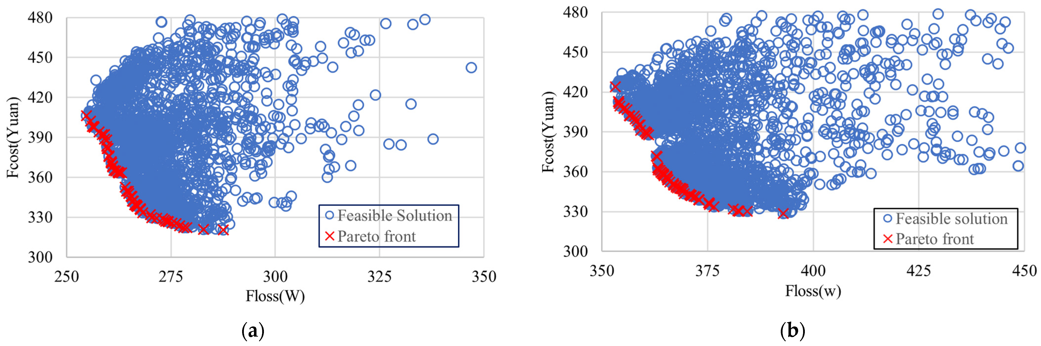
Figure 8a and Figure 8b show the Pareto frontiers obtained when considering and neglecting PWM-induced harmonic losses, respectively. It can be seen that F_loss^w computed when considering PWM-induced harmonic losses are much larger than those obtained when neglecting them, showing that PWM-induced harmonic losses account for a significant proportion of the total losses.

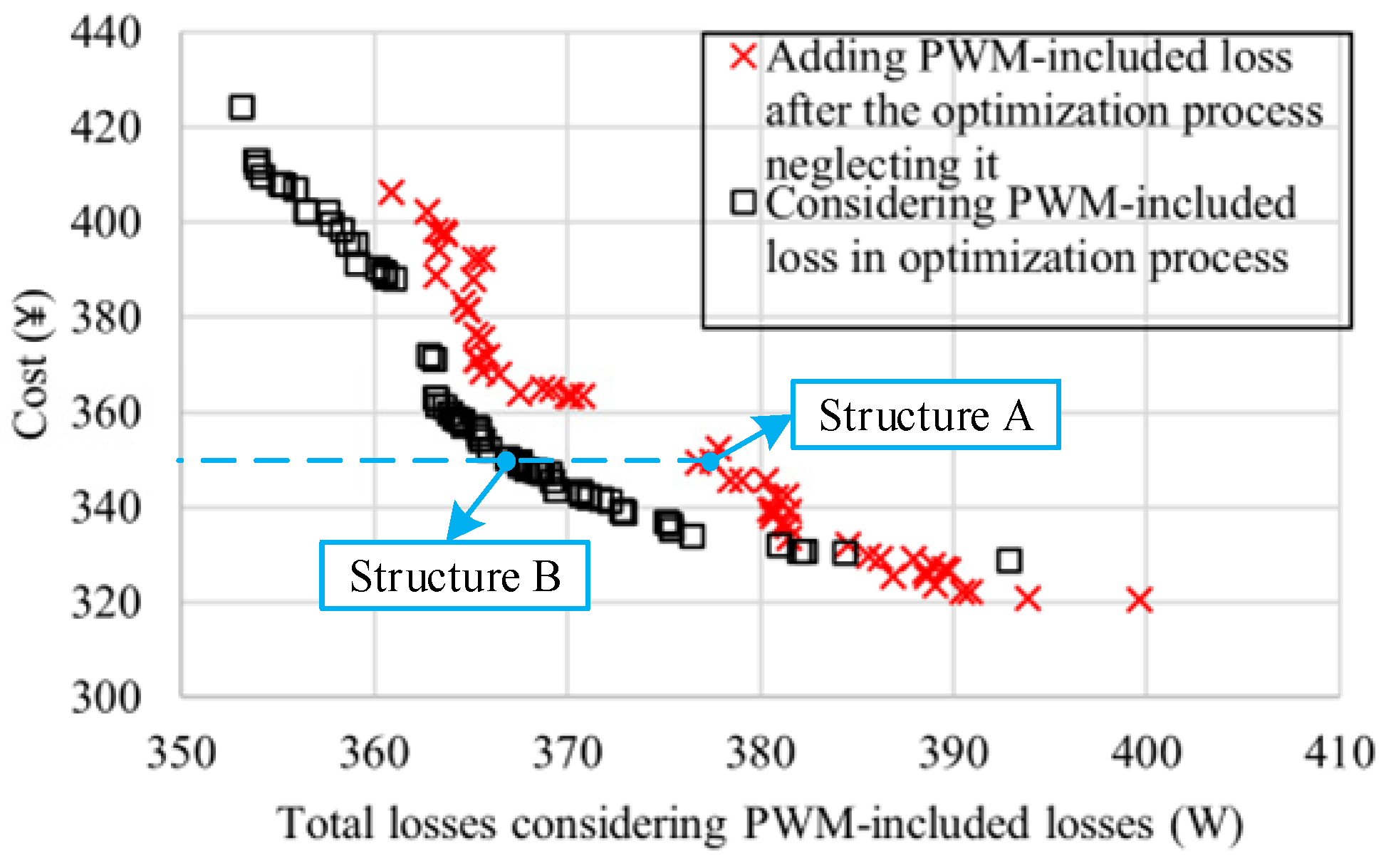
To enable a more comprehensive comparison between the two Pareto frontiers presented in Figure 8, the PWM-induced harmonic losses associated with each point on the frontier in Figure 8a are first computed separately. These harmonic loss values are subsequently added to the corresponding losses under SCS supply, yielding an updated frontier. This revised frontier is then compared against the directly obtained Pareto front from Figure 8b, with the result shown in Figure 9.

Several observations can be made from this comparison. First, after augmenting the original frontier from Figure 8a with the PWM-induced harmonic losses, the resulting solution set becomes unevenly distributed across the design space. Second, dominance relationships emerge among the solutions in this updated set, indicating that it no longer satisfies the criteria for a true Pareto-optimal front. Third, when PWM harmonic losses are directly incorporated into the optimization process, the resulting solutions generally exhibit better Pareto domination rankings than those obtained by optimizing exclusively under SCS excitation. These findings collectively suggest that PWM-induced harmonic losses must be explicitly accounted for when performing efficiency optimization of IPMSMs driven by PWM voltage source inverters.

To accelerate the computations, all parametric sweep FEA simulations were run in parallel using nine CPU cores. The population size in the genetic algorithm was configured as 100 individuals (ten times the number of design variables), and a total of 60 generations evolved. The hardware platform used for all simulations was a workstation equipped with an Intel(R) Xeon(R) Gold 6226R processor running at 2.90 GHz with 32 cores. The total optimization time amounted to 59.3 h when PWM harmonic losses were omitted, increasing to 76.6 h when they were included. Thanks to the fast harmonic loss calculation method adopted in this work, the computational overhead incurred by considering PWM effects was limited to a 22.6% increase.

To quantitatively demonstrate the improvement in motor performance achievable by considering PWM-induced harmonic losses during the optimization process, two structures with identical costs are selected for detailed comparative analysis in Figure 9. Structure A is obtained when neglecting PWM-induced harmonic losses, while structure B is obtained when considering them. Detailed comparison of the two structures is presented in

Table 10. Comparison of two structures obtained with different optimization methods.

	Parameters	Structure A	Structure B
Variables	ang1	46.69°	50.98°
	ang2	31.01°	30.49°
	BS	4.65 mm	5.12 mm
	HS	1.57 mm	1.30 mm
	Hy	17.48 mm	17.64 mm
	LM1	13.85 mm	12.71 mm
	WM1	3.77 mm	4.21 mm
	LM2	22.12 mm	19.71 mm
	WM2	4.63 mm	5.66 mm
	L_axis	72.17 mm	70.62 mm
Weighted average lossesunder SCS supply	PM, PPMscs	0.57 W	0.52 W
	Copper, Pcsscs + Pcescs	118.81 W	139.79 W
	Iron, Pihysscs + Piedscs	144.82 W	127.21 W
	Total, PSCS	264.20 W	267.52 W
Weighted averagePWM-induced harmonic losses	PM, PPWMPM	46.71 W	36.88 W
	Copper, PPWMCu	21.38 W	16.46 W
	Iron, PPWMst + PPWMro	45.64 W	45.66 W
	Total, PPWM	113.73 W	99.00 W
Total loss	PSCS + PPWM	377.93 W	366.51 W
Cost	PM	179.2 yuan	187.0 yuan
	Copper	58.6 yuan	52.94 yuan
	Iron	114.7 yuan	112.2 yuan
	Total	352.4 yuan	352.2 yuan

. P_PWM accounts for approximately 30% of the total losses. Although P_SCS of structure A is smaller than that of structure B, P_PWM of structure B is much small. Hence, the total loss of structure A is larger. The PWM-induced harmonic losses in PMs are smaller in structure B, because the widths of PMs in structure B are smaller than those of structure A and there are fewer high-frequency flux linkages generated by harmonic voltages passing through the PMs. The PWM-induced harmonic losses in PMs can be further reduced by PM segmentation [16], which, however, may also increase the processing cost and is not discussed here for due to the paper length limitation.

By comparing and analyzing the loss distribution of the two motors, it is evident that the SCS loss of the motor optimized only considering SCS losses (Structure A) is lower than that of the motor optimized for PWM-induced harmonic loss (Structure B). However, its total loss is higher than that of structure B. This is because structure B takes into account the optimization of PWM-induced losses, resulting in a smaller copper conductor area compared to structure A, which is optimized only for SCS loss. The reduction in copper area significantly increases the AC copper loss, but at the same time, the increase in the PM area reduces the PWM-induced harmonic losses of the PM. Therefore, when the cost difference is 0.07%, the total loss is reduced by 3.0%.

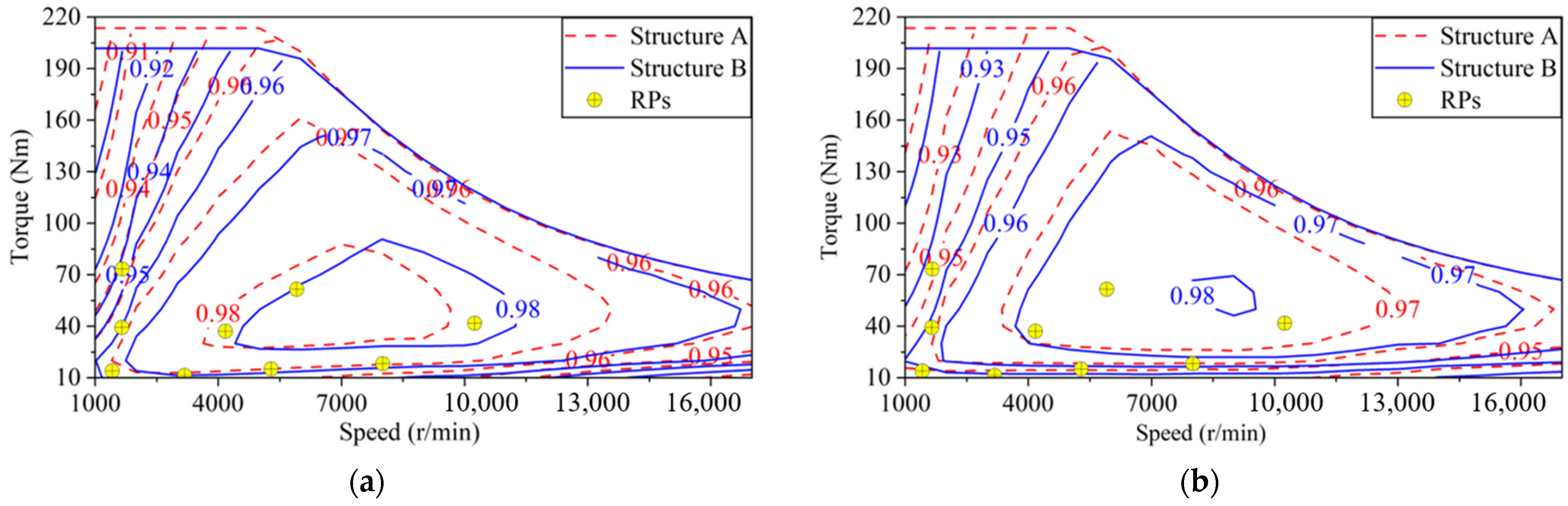
As can be seen from Figure 10, it can be concluded that before considering the PWM-included loss, the high-efficiency regions of Structure A and Structure B are similar. After considering the weights of the nine RPs, the total loss of Structure A is 1.2% less than Structure B. After considering the PWM-included loss, the area of the high-efficiency region for Structure B is greater than Structure A. Furthermore, after considering the weights of the 9 RPs, the total loss of Structure B is 3.11% less than that of Structure A.

F_output^w is the weighted average output power at nine representative points, which is calculated as:

$$\begin{array}{l}{F}_{output}^w={\displaystyle \sum _{i=1}^9\frac{2\pi n_i{\tau }_i\cdot w_i}{60}}\\ \eta ={\displaystyle \frac{F_{output}^w}{(F_{output}^w+F_{loss}^w)}}\end{array}$$

(13)

where $n_i$ is the speed at point i, ${\tau }_i$ is the Torque at point I, and $\eta$ represents the optimized motor efficiency. The efficiency of structure B increased by 0.1% compared to structure A after considering PWM harmonic losses. Therefore, considering PWM harmonic losses is beneficial in terms of optimizing efficiency.

5. Conclusions

In the geometric parameter optimization design of IPMSM, to simulate the motor characteristics under specific driving conditions, the corresponding motor torque and speed are calculated based on the vehicle dynamics model. Using the k-means clustering method, nine representative operating points are extracted. By using small-signal THFEA to extract the loss coefficients associated with harmonic voltages and AC copper losses due to harmonics, and considering the influence of fundamental current and rotor position on the loss coefficients, the rapid calculation of PWM-included harmonic AC copper losses across all operating conditions is achieved. Based on this, a complete rapid calculation process for PWM harmonic losses is established, and by combining the loss calculation results under SCS supply, the correction of the efficiency map is completed.

Meanwhile, further research is still needed for the calculation of AC copper losses in the end windings. By comparing the optimization results with those calculated under only SCS input, the optimization considering PWM harmonic losses obtains a more superior and evenly distributed Pareto frontier, with higher efficiency. At the cost of only a 22.6% increase in calculation time, with the same total cost of the IPMSM, a 3.11% reduction in the total motor losses is achieved.

References

1. Huynh, T.A.; Hsieh, M.-F. Comparative study of PM-assisted SynRM and IPMSM on constant power speed range for EV applications. IEEE Trans. Magn. 2017, 53, 8211006. [Google Scholar] [CrossRef]
2. Lazari, P.; Wang, J.; Chen, L. A computationally efficient design technique for electric-vehicle traction machines. IEEE Trans. Ind. Appl. 2014, 50, 3203–3213. [Google Scholar] [CrossRef]
3. Carraro, E.; Morandin, M.; Bianchi, N. Traction PMASR motor optimization according to a given driving cycle. IEEE Trans. Ind. Appl. 2016, 52, 209–216. [Google Scholar] [CrossRef]
4. Yu, Y.; Wang, C.; Wang, W.; Lu, K.; Chen, Z.; Zhao, D.; Ju, B.-F.; Zhou, S. Determination of elastic constants in unidirectional CFRP laminates using neural networks and laser ultrasonic bulk waves. Compos. Part A Appl. Sci. Manuf. 2026, 207, 109827. [Google Scholar] [CrossRef]
5. Fatemi, A.; Demerdash, N.A.O.; Nehl, T.W.; Ionel, D.M. Large-scale design optimization of PM machines over a target operating cycle. IEEE Trans. Ind. Appl. 2016, 52, 3772–3782. [Google Scholar] [CrossRef]
6. Mahmouditabar, F.; Vahedi, A.; Takorabet, N. Robust design of BLDC motor considering driving cycle. IEEE Trans. Transp. Electrif. 2024, 10, 1414–1424. [Google Scholar] [CrossRef]
7. Ji, J.; Yang, Y.; Ling, Z.; Zhao, W. Multi-objective optimization of interior permanent magnet machine for heavy-duty vehicle direct-drive applications. IEEE Trans. Energy Convers. 2022, 37, 1946–1954. [Google Scholar] [CrossRef]
8. Salameh, M.; Brown, I.P.; Krishnamurthy, M. Fundamental evaluation of data clustering approaches for driving cycle-based machine design optimization. IEEE Trans. Transp. Electrif. 2019, 5, 1395–1405. [Google Scholar] [CrossRef]
9. Shao, L.; Tavernini, D.; Karci, A.; Sorniotti, A. Design and optimisation of energy-efficient PM-assisted synchronous reluctance machines for electric vehicles. IET Electr. Power Appl. 2023, 17, 788–801. [Google Scholar] [CrossRef]
10. Kim, H.-J.; Lee, C.-S. Shape parameters design for improving energy efficiency of IPM traction motor for EV. IEEE Trans. Veh. Technol. 2021, 70, 6662–6673. [Google Scholar] [CrossRef]
11. Sizov, G.Y.; Ionel, D.M.; Demerdash, N.A.O. Modeling and parametric design of permanent-magnet AC machines using computationally efficient finite-element analysis. IEEE Trans. Ind. Electron. 2012, 59, 2403–2413. [Google Scholar] [CrossRef]
12. Wu, X.; Zhang, Y.-T.; Lai, K.-W.; Yang, M.-Z.; Yang, G.-L.; Wang, H.-H. A novel centralized federated deep fuzzy neural network with multi-objectives neural architecture search for epistatic detection. IEEE Trans. Fuzzy Syst. 2024, 33, 94–107. [Google Scholar] [CrossRef]
13. Miyama, Y.; Hazeyama, M.; Hanioka, S.; Watanabe, N.; Daikoku, A.; Inoue, M. PWM carrier harmonic iron loss reduction technique of permanent-magnet motors for electric vehicles. IEEE Trans. Ind. Appl. 2016, 52, 2865–2871. [Google Scholar] [CrossRef]
14. Wu, X.; Wang, H.; Tan, W.; Wei, D.; Shi, M. Dynamic allocation strategy of VM resources with fuzzy transfer learning method. Peer-To-Peer Netw. Appl. 2020, 13, 2201–2213. [Google Scholar] [CrossRef]
15. Yamazaki, K.; Abe, A. Loss investigation of interior permanent-magnet motors considering carrier harmonics and magnet eddy currents. IEEE Trans. Ind. Appl. 2009, 45, 659–665. [Google Scholar] [CrossRef]
16. Zhu, S.; Wang, H.; Zhang, J.; Lu, Z.; Cheng, M. Fast calculation of carrier harmonic loss in permanent magnet of IPMSM under PWM VSI supply over entire working range. IEEE Trans. Energy Convers. 2019, 34, 1581–1592. [Google Scholar] [CrossRef]
17. Zhu, S.; Zeng, F.; Lu, J.; Yu, J.; Liang, X. Simplified engineering calculation of efficiency map of interior permanent magnet synchronous machines with hairpin windings considering PWM-induced harmonic losses. Trans. China Electrotech. Soc. 2022, 37, 5687–5703. [Google Scholar]
18. Yamazaki, K.; Togashi, Y.; Ikemi, T.; Ohki, S.; Mizokami, R.; Mizokami, R. Reduction of inverter carrier harmonic losses in interior permanent magnet synchronous motors by optimizing rotor and stator shapes. IEEE Trans. Ind. Appl. 2019, 55, 306–315. [Google Scholar] [CrossRef]
19. Yamazaki, K.; Iida, K.; Terai, Y. Fast estimation of harmonic losses caused by inverter carrier in interior permanent-magnet synchronous motors by using combination of time- and frequency-domain finite-element analyses. IEEE Trans. Magn. 2020, 56, 8211006. [Google Scholar] [CrossRef]
20. He, Q.; Qu, C.; Zuo, W. Planning Waste-to-Energy-Coupled AI Data Centers Through Grade-Matched Cooling and Corridor Screening. Thermo 2026, 6, 28. [Google Scholar] [CrossRef]
21. Luo, F.; Wang, S.; Lv, Y.; Mu, R.; Fo, J.; Zhang, T.; Xu, J.; Wang, C. Domain knowledge-enhanced graph reinforcement learning method for Volt/Var control in distribution networks. Appl. Energy 2025, 398, 126409. [Google Scholar] [CrossRef]
22. Zhu, S.; Dong, J.; Li, Y.; Wei, H. Fast calculation of carrier harmonic iron losses caused by pulse width modulation in interior permanent magnet synchronous motors. IET Electr. Power Appl. 2020, 14, 1163–1176. [Google Scholar] [CrossRef]
23. Fan, X.; Li, D.; Kong, W.; Cao, L.; Qu, R.; Yin, Z. Fast calculation of strand eddy current loss in inverter-fed electrical machines. IEEE Trans. Ind. Electron. 2023, 70, 4640–4650. [Google Scholar] [CrossRef]
24. Han, P.; Liang, J.; Gottipati, P.; Solveson, M. Generalized high-frequency small-signal modeling of electric machines using electromagnetic FEA. In Proceedings of the 2023 IEEE Energy Conversion Congress and Exposition (ECCE), Nashville, TN, USA, 29 October–2 November 2023; pp. 4105–4112. [Google Scholar] [CrossRef]
25. Zhu, S.; Zeng, F.; Lu, J.; Chu, Z. Fast Driving Cycle Efficiency Optimization of an IPMSM with Hairpin Windings Considering PWM-Induced Losses; ICEMS: Zhuhai, China, 2023; pp. 2988–2995. [Google Scholar]
26. Lin, D.; Zhou, P.; Fu, W.N.; Badics, Z.; Cendes, Z.J. A dynamic core loss model for soft ferromagnetic and power ferrite materials in transient finite element analysis. IEEE Trans. Magn. 2004, 40, 1318–1321. [Google Scholar] [CrossRef]
27. Kwak, J.; Castellazzi, A. State-of-the-art 800 V electric drive systems: Inverter-machine codesign for energy efficiency optimization. Electronics 2023, 12, 3063. [Google Scholar] [CrossRef]
28. Chen, X.; Wang, J.; Sen, B.; Lazari, P.; Sun, T. A high-fidelity and computationally efficient model for interior permanent-magnet machines considering the magnetic saturation, spatial harmonics, and iron loss effect. IEEE Trans. Ind. Electron. 2015, 62, 4044–4055. [Google Scholar] [CrossRef]
29. Ge, H.; Miao, Y.; Bilgin, B.; Nahid-Mobarakeh, B.; Emadi, A. Speed Range Extended Maximum Torque Per Ampere Control for PM Drives Considering Inverter and Motor Nonlinearities. IEEE Trans. Power Electron. 2017, 32, 7151–7159. [Google Scholar] [CrossRef]
30. Dai, L.; Gao, J.; Niu, S.; Huang, S. Multi-electromagnetic performance optimization of double-layer interior permanent magnet synchronous machine. IEEE Trans. Ind. Electron. 2024, 71, 14535–14545. [Google Scholar] [CrossRef]
Figure 1. Vehicle profile (time–speed) for CLTC-P driving condition.
Machines 14 00599 g001
Figure 2. IPMSM output torque profile.
Machines 14 00599 g002
Figure 3. Load energy consumption over the torque-speed plane.
Machines 14 00599 g003
Figure 4. Calculation of the cyclic RPs and their associated energy weights using the k-means algorithm with nine clusters.
Machines 14 00599 g004
Figure 5. Illustration of optimization variables for the prototype IPMSM.
Machines 14 00599 g005
Figure 6. Comparison of maximum torque-speed plots.
Machines 14 00599 g006
Figure 7. Comparison of copper losses calculated with TSFEA using different time steps when id is −105.74 A, iq is 67.52 A, and speed is 10,241 r/min.
Machines 14 00599 g007
Figure 8. Comparison of optimization results: (a) Neglecting PWM-induced losses; (b) considering PWM-induced losses.
Machines 14 00599 g008
Figure 9. Comparison of Pareto frontiers obtained by different methods.
Machines 14 00599 g009
Figure 10. Compare the efficiency maps with RPs of Structure A and Structure B: (a) neglecting PWM-included losses; (b) considering PWM-included losses.
Machines 14 00599 g010