Article

Learning-Based Optimal Control for Multiple Fixed-Wing UAVs with Prescribed Performance

1
College of Air Traffic Control and Navigation, Air Force Engineering University, Xi’an 710051, China
2
Key Laboratory of Road and Traffic Engineering of the Ministry of Education, College of Transportation, Tongji University, Shanghai 201804, China
*
Author to whom correspondence should be addressed.
Machines 2026, 14(6), 583; https://doi.org/10.3390/machines14060583
Submission received: 23 April 2026 / Revised: 20 May 2026 / Accepted: 22 May 2026 / Published: 25 May 2026
(This article belongs to the Special Issue Intelligent Control Techniques for Unmanned Aerial Vehicles)

Abstract

Fixed-wing unmanned aerial vehicle formation control confronts the dual challenges of achieving optimal performance amidst complex nonlinear dynamics and ensuring flight safety by constraining tracking errors. Existing reinforcement learning methods, though effective for optimal control, often overlook these critical safety constraints, which constitutes a serious shortcoming in safety-critical swarm operations where unmanned aerial vehicles confront highly nonlinear dynamics, unknown disturbances, and limited model knowledge, and these practical necessity drives us to synergistically integrate two previously separated techniques. To address this issue, this paper proposes a safe optimal control framework that synergistically integrates prescribed performance control with an actor–critic RL scheme. Specifically, a simplified actor–critic architecture is developed to derive a near-optimal controller for the coupled position–attitude dynamics without requiring an accurate model, thereby enhancing energy efficiency. Concurrently, the prescribed performance control is employed to transform the constrained formation error dynamics into an unconstrained system, guaranteeing that safety distances are strictly maintained. Lyapunov-based analysis proves that all signals in the closed-loop system are semi-globally uniformly ultimately bounded and that formation errors never violate the predefined performance boundaries.

1. Introduction

In recent years, unmanned aerial vehicle (UAV) technology has found extensive application in military reconnaissance, environmental monitoring, and logistics transportation. In particular, fixed-wing UAVs have become critical platforms for cooperative multi-UAV missions due to their long endurance, extended range, and high maneuverability [1,2,3]. Operating multiple fixed-wing UAVs in formation can effectively enhance mission efficiency and system redundancy. However, this simultaneously imposes stricter demands on the robustness and safety of control systems [4,5,6]. On one hand, the dynamics of fixed-wing UAVs are characterized by strong nonlinearity, model uncertainties, and external wind disturbances. In practical fixed-wing UAV systems, structural vibration, damping characteristics, and material properties may also affect control quality [7,8,9]. Lightweight UAV structures are sensitive to vibration, which can degrade sensor accuracy, disturb attitude responses, and reduce formation tracking performance. Recent studies on vibration-aware UAV structures, lightweight composite materials, and sustainable damping materials, such as cork-based composites, indicate that structural damping and material selection are important factors for improving UAV flight stability and control reliability. On the other hand, the necessity to maintain safe inter-UAV distances for collision avoidance requires that control designs explicitly account for constraints on position tracking errors.
For UAV formation control, the investigation of optimal control strategies holds significant theoretical and engineering value. Fixed-wing UAV systems are inherently complex, characterized by strong nonlinearity, multivariable coupling, and model uncertainties. Consequently, formation flight requires not only precise shape maintenance but also the optimization of control performance under energy constraints [10,11,12]. Traditional methods such as the linear quadratic regulator or linear quadratic gaussian struggle to directly address nonlinear dynamics and external disturbances. Furthermore, optimal control problems for nonlinear systems often reduce to solving the Hamilton–Jacobi–Bellman (HJB) equation, which is analytically intractable in practical engineering [13,14,15]. In recent years, reinforcement learning (RL) methods have been increasingly applied to UAV systems due to their potential in solving optimal control problems [16,17,18]. By adopting an actor–critic architecture, RL leverages the function approximation capabilities of neural networks to approximate the HJB equation without relying on an accurate model. This approach yields near-optimal control strategies, which offers a viable pathway for solving optimal control problems in complex nonlinear systems [19,20,21]. For example, the authors in [20] designed a simplified optimal control scheme through constructing the positive definite function with a simple form. In [21], the authors presented an optimized backstepping control scheme for nonlinear strict-feedback systems with unknown dynamic by using the simplified actor–critic architecture. Several recent studies have further advanced robust cooperative control [22] and learning-based swarm control [23]. Nevertheless, they still do not simultaneously address optimality and hard safety constraints. However, most of the aforementioned RL-based methods neglect safety constraints during flight, making them difficult to directly apply to safety-critical formation missions.
Furthermore, safety constraints constitute a critical issue that must be addressed during formation flight [24,25,26]. To avoid collisions, UAVs must maintain safe inter-agent distances, necessitating that position tracking errors be strictly confined within predefined bounds. Prescribed performance control (PPC) addresses this issue by transforming constrained tracking errors into an unconstrained system via predefined performance functions, thereby theoretically guaranteeing that errors satisfy boundary conditions at all times [27,28,29,30]. A prescribed-time PPC method is proposed to ensure docking errors converge to a user-defined domain in [31]. The authors in [32] designed a reconfigurable performance function to solve the control singularity problem of UAV systems under actuator saturation conditions. While this method has been validated in single-UAV flight control, effectively integrating prescribed performance constraints with an RL-based optimal control framework for multi-UAV cooperative formations while simultaneously accounting for the strong nonlinearity of fixed-wing UAVs remains a challenging and active area of research.
Although robust and adaptive control methods have been widely used for UAV formation systems, their primary objective is usually to ensure stability and robustness under uncertainties. For safety-critical fixed-wing UAV swarms, however, the controller must satisfy two requirements simultaneously: strict transient/steady-state bounds on formation errors for collision avoidance, and near-optimal control performance under coupled nonlinear position–attitude dynamics, unknown disturbances, and inaccurate model parameters. Robust/adaptive designs may guarantee boundedness, but they do not explicitly minimize an infinite-horizon performance index and may lead to conservative control actions. On the other hand, RL-based optimal control can approximate the HJB solution and improve control efficiency without an accurate model, but conventional RL schemes do not inherently prevent formation errors from violating safety boundaries during learning and transient maneuvers. PPC is therefore introduced to impose prescribed error constraints, and the actor–critic RL scheme is designed on the transformed unconstrained error dynamics to achieve near-optimal control. This complementary integration is the main motivation of the proposed framework.
Encouraged by the above analysis, this paper aims to combine PPC with RL-based optimal control to develop a safe optimal control framework for fixed-wing UAV formations. This framework is designed to achieve near-optimal formation tracking performance while guaranteeing flight safety. The main contributions are summarized as follows:
  • A simplified actor–critic RL scheme is developed to handle the coupled position–attitude dynamics of fixed-wing UAV. By employing neural networks to approximate the solution to the HJB equation, the proposed method realizes approximate optimal control without relying on an accurate model, which reduces computational complexity and improving control energy efficiency.
  • The prescribed performance function is introduced to impose predefined boundary constraints on formation errors, which ensures that safe inter-UAV distances are rigorously maintained throughout the formation flight and that addresses the limitation of existing RL control methods which typically neglect safety constraints.
  • By using the Lyapunov theory, it is proven that all error signals in the closed-loop system are SGUUB, and that the formation errors remain strictly within the prescribed performance boundaries.
The remainder of this paper is organized as follows. Section 2 presents the UAV dynamics and formation error formulation. Section 3 describes the prescribed performance transformation and the actor–critic RL framework, including the optimal control law, adaptive law, and online learning mechanism. Section 4 provides stability analysis proving SGUUB and prescribed performance bounds. Section 5 shows simulation results, including setup, comparisons, sensitivity, robustness tests, and practical deployment discussions. Appendix A includes the introduction to neural network.

2. Preliminaries

This section introduces the dynamic models of fixed-wing unmanned aerial vehicles and virtual leaders, defines formation tracking errors, and clarifies the control objectives of this paper.

2.1. Dynamics of Fixed-Wing Unmanned Aerial Vehicle

For a multi-UAV system with N UAVs, let N : = { 1 , 2 , , N } represent the set of indices. The motion dynamics of the i-th UAV is formulated as
I ˙ i x = v i cos ψ i cos θ i + l i x I ˙ i y = v i sin ψ i cos θ i + l i y I ˙ i z = v i sin θ i + l i z
where ( I i x , I i y , I i z ) denotes the position of the i-th UAV in an inertia coordinate frame, while v i , ψ i , θ i are velocity, course angle, and pitch angle, respectively. I i x , I i y , I i z denote bounded disturbances in x , y , z axes, respectively.
Considering the autopilots onboard, the time response dynamics of v i , ψ i , θ i are modeled as follows [33,34]:
v ˙ i = ( v i * v i ) ( η v + Δ η v ) ψ ˙ i = ( ψ i * ψ i ) ( η ψ + Δ η ψ ) θ ˙ i = ( θ i * θ i ) ( η θ + Δ η θ )
where v i * , ψ i * and θ i * denote the command velocity, course angle and pitch angle, respectively. η v , η ψ and η θ are the positive time constants associated with velocity-hold loop, course angle-hold loop and pitch angle-hold loop, respectively. Additionally, Δ η v , Δ η ψ , Δ η θ are bounded parameter uncertainties arising from the autopilot dynamics.
The virtual leader is modeled as
r ˙ x = v r sin θ r cos ψ r r ˙ y = v r cos θ r sin ψ r r ˙ z = v r sin θ r
where ( r x , r y , r z ) represents the position of virtual leader. v r is the velocity, ψ r denotes course angle, and θ r is pitch angle of virtual leader.

2.2. Problem Statement

Based on (1) and (3), the relative position and state for UAVs is described by
z i z r = Δ z i r ϕ i ϕ r = Δ ϕ i r
where z i = [ I i x , I i y , I i z ] T , z r = [ r x , r y , r z ] T denote the position vectors of the ith UAV and virtual leader, respectively. Δ z i r R 3 represents their relative position. Similarly, ϕ i = [ v i , ψ i , θ i ] T , ϕ r = [ v r , ψ r , θ r ] T stand for the flight state vectors of the ith UAV and virtual leader, with Δ ϕ i r = [ Δ v i r , Δ ψ i r , Δ θ i r ] T defining the relative state vector.
Define the position tracking error of the ith UAV as
ω i z = Δ z i r p i r = ω i z x , ω i z y , ω i z z T
where z i r = [ z i r x , z i r y , z i r z ] T is the expected relative position of the ith UAV with respect to virtual leader. z i r , which is specified by the task-driven formation configuration.
Remark 1.
For close UAV formation, practical formation tracking can be achieved by keeping the position error ω z i within a predefined range, where parameters α z i and α z j are chosen to ensure collision avoidance. The relative position between two UAVs is given by Δ z i j = z i z j = ( e z i + p i r ) ( ω z j + p j r ) .
Then, the error system of each UAV is derived as
ξ ˙ i = F i + G i U i + D i
where
ξ i = ω i z x , ω i z y , ω i z z , Δ v i r , Δ ψ i r , Δ θ i r T ,
F i = v i cos ψ i sin θ i v r cos ψ r sin θ r q ˙ i r x v i sin ψ i cos θ i v r sin ψ r cos θ r q ˙ i r y v i sin θ i v r sin θ r q ˙ i r z v ˙ r η v v i x ψ ˙ r η ψ ψ i θ ˙ r η θ θ i ,
G i = 0 0 0 0 0 0 0 0 0 0 0 0 1 0 0 0 0 0 0 0 0 0 0 0 η v 0 0 0 0 0 0 η ψ 0 0 0 0 0 0 η θ 0 0 0 ,
U i = [ v i * , ψ i * , θ i * ] T ,
D i = [ l i x , l i y , l i z , l i v , l i ψ , l i θ ] T .

2.3. Prescribed Performance Control

To ensure flight safety, the tracking error ξ i is designed to be limited within a specified boundary, i.e.,
ζ i < ω i z k < ζ i , ζ i < Δ φ i r < ζ i
where k = x , y , z and φ = v , ψ , θ .
Define the following performance function as
ζ i = ( μ i 0 μ i ) e ρ t + μ i ,
where ρ , μ i 0 , μ i are positive constants. ζ i 0 = ζ i ( 0 ) with ζ i ( 0 ) < ω i z k ( 0 ) < ζ i ( 0 ) and ζ i ( 0 ) < Δ φ i r ( 0 ) < ζ i ( 0 ) .
As the design of Δ φ i r follows the same logic as ω i z k , the details are not repeated here. Instead, only the case for ω i z k is illustrated. Construct the error transformation as follows [35]:
e i k = ln ζ i + ω i z k ζ i ω i z k , t 0
Take the derivative of (7), one gets
d e i k d t = e i k ζ i ζ ˙ i + e i k ω i z k ω ˙ i z k = 2 ω i z k ζ i 2 ω i z k 2 ζ ˙ i + 2 ζ i ζ i 2 ω i z k 2 ω ˙ i z k = Γ i k + v i k ω ˙ i z k
where Γ i k = 2 ω i z k ζ i 2 ω i z k 2 ζ ˙ i , and v i k = 2 ζ i ζ i 2 ω i z k 2 .
Then, the error transformation dynamics is given by
e ˙ i = Γ i + v i ξ ˙ i z
Taking (6) in (9), it yields
e ˙ i = F v i + G v i U i + D v i
where F v i = v i F i , G v i = v i G i , and D v i = v i D i + Γ i .
Objectives: The focus of this work is to devise an optimal formation control protocol for multiple fixed-wing UAVs system (1) such that
(1)
The formation tracking error of the fixed-wing UAVs remains strictly within the prescribed performance boundary.
(2)
All closed-loop signals of the fixed-wing UAVs are SGUUB.
To fulfill these objectives, the controller design relies on the following definition and assumption as prerequisites.
Definition 1 ([20]).
(Semiglobally Uniformly Ultimately Bounded (SGUUB)) The solution x ( t ) R n of nonlinear system x ˙ ( t ) = f ( x , t ) is said to be SGUUB, if the inequality x ( t ) ρ holds for t > T ( ρ , x ( 0 ) ) , where ρ and T ( ρ , x ( 0 ) ) are constants, and Ω is a compact set.
Lemma 1 ([36,37]).
Design a a positive continuous function L ( t ) R with the initial value L ( 0 ) . If it satisfies
L ˙ ( t ) ν L ( t ) + σ ,
where constants ν and σ are positive, then the following relationship holds:
L e ν t L ( 0 ) + σ ν ( 1 e ν t ) .

3. Optimal Controller Design and Stability Analysis

This section reviews the construction of the adaptive optimal controller and discusses the system stability.

3.1. Optimal Controller Design

To enforce safe distance constraints, we map the constrained tracking error to an unconstrained variable via PPC. This allows later optimal control design to be performed on the unconstrained dynamics.
Define the performance index function as
J i ( e i ) = t V i ( e i , U i ) d s
where V i ( e i , U i ) = e i T e i + U i T U i denotes the cost function.
The optimal performance index function is prescribed as
J i * ( e i ) = t V i ( e i , U i * ) d s = min U i Ψ ( Ω U ) t V i ( e i , U i ) d s
where Ω U R 3 is the compact set, and U i * is the optimal position control signal of UAVs.
Based on (12), the HJB equation can be formulated as
H 1 e i , U i * , d J i * d e i = e i T e i + U i * T U i * + d J i * d e i e ˙ i
Solving the equation ( H 1 / U i * ) = 0 yields the optimal UAV position control U i * as
U i * = 1 2 d J i * d e i G v i .
Decomposing the term ( d J 1 * / d e i ) yields two parts as follows:
d J i * d e i = 2 c i e i + e i Ψ ^ i | | ϕ i | | 2 2 a i + J i 0 ( e i )
in which c i > 0 is the design parameter and J i 0 ( e i ) = 2 c i e i + e i Ψ ^ i | | ϕ i | | 2 2 a i + d J i * / d e i .
Then, the optimal control U i * is given by
U i * = G v i 1 c i e i + e i Ψ ^ i | | ϕ i | | 2 2 a i G v i 2 J i 0 ( e i )
The unknown term J 1 0 ( e ξ 2 ) is continuous, so it can be expressed by NN in the following form:
J 1 0 ( e i ) = χ a i T ϕ i ( e i ) + δ i ( e i )
where χ a i , ϕ i , and δ i are the ideal weight, the basis function vector and the approximation error, respectively. And the details of NN is given in Appendix A.
Instead of solving the HJB equation analytically, we use an actor--critic RL architecture to approximate the optimal value function and policy online, using only measured signals.
Inserting (15) into (16) and (17) results in
d J i * d e i = 2 c i e i + e i Ψ ^ i | | ϕ i | | 2 2 a i + ( χ a i T ϕ i + δ i )
U i * = G v i 1 c i e i + e i Ψ ^ i | | ϕ i | | 2 2 a i G v i 2 ( χ a i T ϕ i + δ i )
Since the ideal weight χ a i is an unknown constant matrix, it makes the optimal UAV position control unavailable. For deriving the valid optimized control, the RL is performed by constructing the following both critic and actor.
Given that the ideal weight matrix χ a i is unknown, the optimal control input (19) is not directly realizable. To address this, we employ an RL algorithm that utilizes critic and actor structures to approximate the optimal control.
The critic used for performance evaluation is given by
d J ^ i * d e i = 2 c i e i + e i Ψ ^ i | | ϕ i | | 2 2 a i + χ ^ c i T ϕ i
where d J ^ i * / d e i is the estimation of ( d J i * / d e i ) . And the critic NN weight χ ^ c i is updated by the following law:
χ ^ ˙ c i = k c i ϕ i ϕ i T χ ^ c i
where k c i is a positive parameter.
The actor used for performing the control action is given by
U i ^ * = G v i 1 c i e i + e i Ψ ^ i | | ϕ i | | 2 2 a i G v i 2 χ ^ a i T ϕ i
where the actor NN weight χ ^ c i is updated by the following law:
χ ^ ˙ a i = ϕ i ϕ i T k a i χ ^ a i χ ^ c i + k c i χ ^ c i
where k a i is a positive parameter.
Parameters k c i and k a i are tuned to fulfill the requirements listed below:
k a i > 1 2 , k a i > k c i > 1 2 k a i .
Remark 2.
Formation flight of fixed-wing UAVs imposes high computational demands. Traditional optimal control methods struggle with nonlinear dynamics and the intractable HJB equation, leading to heavy online computation. By adopting simplified optimal control strategies, such as using elementary positive definite functions or reduced actor--critic structures, the computational burden can be significantly reduced. This enables real-time implementation without compromising formation performance.
Remark 3.
Online learning mechanism of actor–critic networks is displayed as follows: (i) The critic network takes the transformed error ϵ i as input and outputs the approximate value function V ^ i = χ ^ c i ϕ i ( ϵ i ) , with weight update rule χ ^ ˙ c i = k c i ϕ i e i G v i derived from minimizing the Bellman residual. (ii) The actor network outputs the approximate optimal control U ^ i = 1 2 R 1 G v i χ ^ a i ϕ i , and its weights are updated as χ ^ ˙ a i = k a i ϕ i ( χ ^ a i χ ^ c i ) , forcing the actor to synchronize with the critic and thereby approach the optimal policy. (iii) The learning runs online: at each sampling instant, the RBF basis functions are computed from the current error e i , and both networks update their weights simultaneously without offline training or experience replay.

3.2. Stability Analysis

This section serves to confirm the validity of the presented optimal control approach.
Theorem 1.
Consider the fixed-wing UAV system with prescribed performance described by Equation (1). If the assumption in Lemma 1 holds, then under the joint action of the designed controller (22), critic NN (21), and actor NN (23), it can be guaranteed that:
(1) 
The formation error can converge to a neighborhood around zero.
(2) 
All signals of the closed-loop system are semi-globally uniformly ultimately bounded.
Proof. 
To demonstrate the stability of the system, the Lyapunov function is constructed as
L i ( t ) = 1 2 e i T e i + 1 2 Tr χ ˜ c i T χ ˜ c i + 1 2 Tr χ ˜ a i T χ ˜ a i + 1 2 Tr Ψ ˜ i T Ψ ˜ i
where χ ˜ c i = χ ^ c i χ c i and χ ˜ a i = χ ^ a i χ a i denote the critic and actor NN weight errors, respectively.
The time derivative of L i is calculated as
L ˙ i = e i T ( D i + G v i U i ) k c i Tr χ ˜ c i T ϕ i ϕ i T χ ^ c i Tr χ ˜ a i T ϕ i ϕ i T k a i χ ^ a i χ ^ c i + k c i χ ^ c i + 1 2 Tr Ψ ˜ i T Ψ ^ ˙ i
where D i = F v i + D v i .
Due to the unknown value of D i , we use NN to obtain the following approximate form:
D i = W i ϕ i + δ i
According to Young’s inequality, it yields that
e i T D i e i T e i Ψ i | | ϕ i | | 2 2 a i + a i 2 2 + e i T e i 2 + δ ¯ i 2 2
where Ψ i = | | W i | | 2 .
According to (22), one has
L ˙ i c i e i T e i e i T e i Ψ ^ i | | ϕ i | | 2 2 a i G i 2 e i T χ ^ a i T ϕ i + e i T e i Ψ i | | ϕ i | | 2 2 a i k c i Tr χ ˜ c i T ϕ i ϕ i T χ ^ c i Tr χ ˜ a i T ϕ i ϕ i T k a i χ ^ a i χ ^ c i + k c i χ ^ c i + 1 2 Tr Ψ ˜ i T Ψ ^ ˙ i + a i 2 2 + e i T e i 2 + δ ¯ i 2 2
where | | G v i | | 2 = G i .
To handle the unknown bound of NN approximation errors, we introduce an adaptive parameter Ψ ^ i that estimates the squared ideal weight norm, reducing computational load. Design the adaptive law as
Ψ ^ ˙ i = b i Ψ ^ i + e i T e i | | ϕ i | | 2 2 a i
where Ψ ^ i Ψ i = Ψ ˜ i .
Using the relations of χ ˜ a i and χ ˜ c i , one obtains
G i 2 e i T χ ^ a i T ϕ i G i 4 e i T e i + G i 4 Tr χ ^ a i T ϕ i ϕ i T χ ^ a i Tr χ ˜ a i T ϕ i ϕ i T χ ^ a i = 1 2 Tr χ ˜ a i T ϕ i ϕ i T χ ˜ a i + 1 2 Tr χ ^ a i T ϕ i ϕ i T χ ^ a i 1 2 Tr χ a i T ϕ i ϕ i T χ a i Tr χ ˜ c i T ϕ i ϕ i T χ ^ c i = 1 2 Tr χ ˜ c i T ϕ i ϕ i T χ ˜ c i + 1 2 Tr χ ^ c i T ϕ i ϕ i T χ ^ c i 1 2 Tr χ c i T ϕ i ϕ i T χ c i
In view of condition (24) and Young’s inequality, one gets
( k a i k c i ) Tr χ ˜ a i T ϕ i ϕ i T χ ^ c i k a i k c i 2 Tr χ ˜ a i T ϕ i ϕ i T χ ˜ a i + k a i k c i 2 Tr χ ^ c i T ϕ i ϕ i T χ ^ c i
Based on the above inequalities, it yields
L ˙ i ( 2 c i G i 2 1 ) e i T e i 2 b i Ψ ˜ i Ψ ˜ i 2 + a i 2 2 + δ ¯ i 2 2 k c i 2 Tr χ ˜ c i T ϕ i ϕ i T χ ˜ c i k c i 2 Tr χ ˜ a i T ϕ i ϕ i T χ ˜ a i + k c i 2 Tr χ c i T ϕ i ϕ i T χ c i + k c i 2 Tr χ a i T ϕ i ϕ i T χ a i ( k a i 2 G i 4 ) Tr χ ^ a i T ϕ i ϕ i T χ ^ a i ( k c i k a i 2 ) Tr χ ^ c i T ϕ i ϕ i T χ ^ c i
Further, the inequality (32) can be written as
L ˙ i ( 2 c i G i 2 1 ) e i T e i 2 b i Ψ ˜ i Ψ ˜ i 2 + C i k c i 2 λ ϕ i min Tr χ ˜ c i T χ ˜ c i k c i 2 λ ϕ 1 min Tr χ ˜ a i T χ ˜ a i
where λ ϕ 1 min is the minimal eigenvalue of ϕ i ϕ i T , C i ( t ) = k c i 2 | | χ c i T ϕ i | | 2 + k c i 2 | | χ a i T ϕ i | | 2 + a i 2 2 + δ ¯ i 2 2 .
Terms of C i ( t ) are bounded, which implies the existence of a constant σ i satisfying | C i ( t ) | σ i .
Defining ν i = min { 2 c i G i 2 1 , b i , k c i λ ϕ i min } , we have
L ˙ i ( t ) ν i L i ( t ) + σ i .
Applying Lemma 1 to (34) yields
L ( t ) e ν t L ( 0 ) + σ ν 1 e ν t .
Inequality (35) implies that all error signals are semi-globally uniformly ultimately bounded, and the tracking errors can achieve ideal accuracy through adjustment parameters. The proof is completed.□
To clarify the novelty of our work, we have proposed the Table 1 to clarify the novelty of our work. In particular, the added table summarizes the main differences among robust/adaptive UAV control, conventional actor–critic UAV control, PPC-based UAV control, existing RL-PPC control, and the proposed method. It compares these methods in terms of their main advantages, limitations, and relevance to the present work, thereby making the novelty of our PPC-based actor–critic framework more explicit. These revisions explicitly highlight the methodological advances of the proposed framework beyond existing RL and PPC control methods.

4. Simulation Results

In this section, a simulation experiment is designed and implemented to verify the effectiveness of the proposed optimal method in multi-UAV formation control.
Simulation Environment: The hardware-in-the-loopexperimental platform, supported by Beijing Links Co., Ltd., is established to validate the proposed learning-based safety control strategy for UAV formation tracking. The platform comprises three core functional units: a development computer running MATLAB R2026b, Tacview v1.9.5, and RTSimPlus 2024 for 3D visualization and real-time simulation management; a flight controller that executes the proposed control strategy and transmits control commands to the real-time simulator via the serial port; and a real-time simulator that models the multi-UAV dynamics, communicates with the development computer over Ethernet, and exchanges state information (including position, velocity, and attitude) with the flight controller through the same serial port. Operating at a time step of 0.01 s, the testbed accounts for the actual computational capability of the flight controller and introduces realistic perturbations into the closed-loop UAV system, thereby providing a practical environment for experimental validation.
Figure 1 shows the communication topology used in the simulation, which is generated according to the predefined information-exchange structure among one virtual leader and four follower UAVs. The nodes represent UAV agents, and the arrows indicate the direction of information flow.

4.1. Parameter Settings

In UAV formation tasks, the initial positions of the virtual leader and four followers are set to create a dispersed spatial configuration, which tests the convergence capability of the formation control scheme. Specifically, the virtual leader starts at z r ( 0 ) = [ 30 , 0 , 500 ] T m, while the followers are initially placed at z 1 ( 0 ) = [ 5 , 5 , 590 ] T m, z 2 ( 0 ) = [ 35 , 30 , 600 ] T m, z 3 ( 0 ) = [ 23 , 25 , 594 ] T m, and z 4 ( 0 ) = [ 54 , 25 , 600 ] T m. All UAVs share the same initial velocity of 8 m/s, and initial course and pitch angles of 0 and 0 , respectively. The autopilot constants are chosen as η v = 1 , η ψ = 10 , and η θ = 10 . The prescribed performance function is designed as ζ i ( t ) = ( 4 0.2 ) e 0.5 t + 0.2 , i = 1 , , 4 , where the initial bound 4 ensures a large enough safe region, the steady-state bound 0.2 guarantees ultimate tracking precision, and the exponential rate 0.5 dictates the minimum convergence speed. The desired relative positions of the four followers with respect to the virtual leader are selected as p 1 r = [ 20 , 0 , 0 ] T m, p 2 r = [ 48 , 28 , 0 ] T m, p 3 r = [ 50 , 32 , 0 ] T m, and p 4 r = [ 80 , 32 , 0 ] T m.
Both the critic and actor neural networks are designed with seven nodes, a moderate size that balances approximation capability and computational load. The initial weight vectors for the critic networks are set as ϕ ^ 1 ( 0 ) = [ 0.8 , 0.8 , 0.8 , 0.7 , 0.7 , 0.7 , 0.7 ] T , ϕ ^ 2 ( 0 ) = [ 0.7 , 0.7 , 0.7 , 0.7 , 0.7 , 0.75 , 0.75 ] T , ϕ ^ 3 ( 0 ) = [ 0.6 ] 7 × 1 , and ϕ ^ 4 ( 0 ) = [ 0.55 ] 7 × 1 . The initial actor weight vectors are chosen as Ψ ^ 1 ( 0 ) = [ 0.45 ] 7 × 1 , Ψ ^ 2 ( 0 ) = [ 0.6 ] 7 × 1 , Ψ ^ 3 ( 0 ) = [ 0.7 ] 7 × 1 , and Ψ ^ 4 ( 0 ) = [ 0.85 ] 7 × 1 . These values are intentionally diversified across followers to examine the robustness of the learning scheme against different initialization conditions.

4.2. Simulation Verification

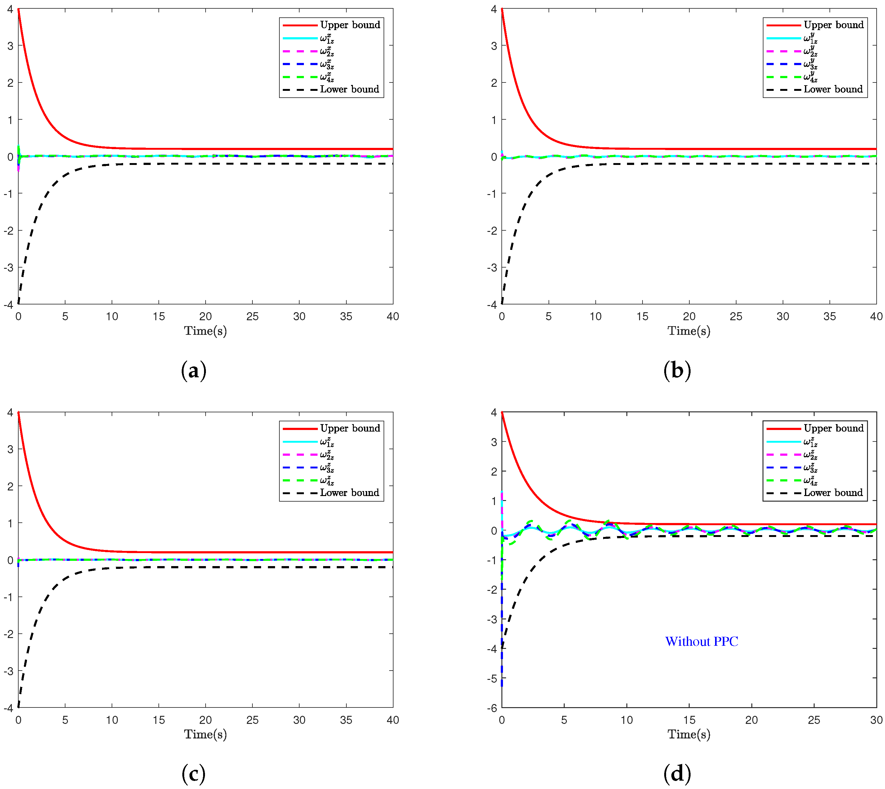
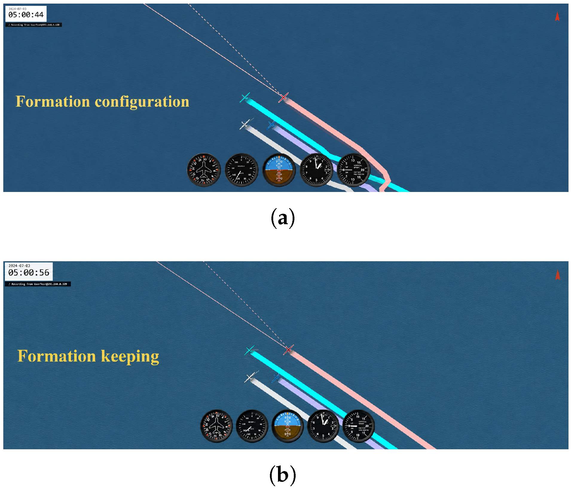
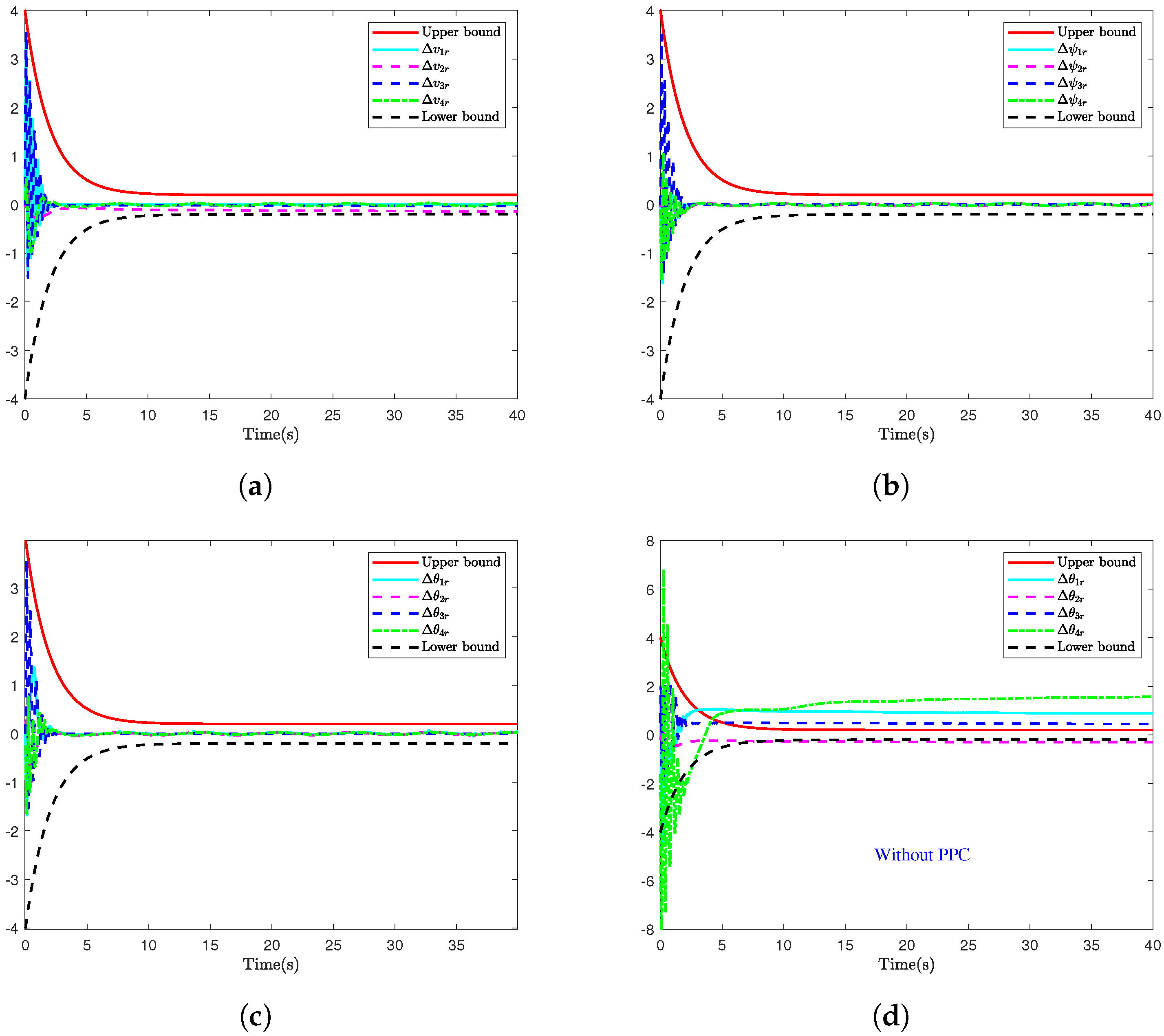
The effectiveness of the proposed optimal formation control strategy for fixed-wing UAVs is clearly demonstrated in Figure 2, Figure 3, Figure 4, Figure 5, Figure 6 and Figure 7. Specifically, Figure 2 is produced using Tacview based on the simulated three-dimensional UAV trajectories. It illustrates the spatial formation evolution of the virtual leader and four followers. Figure 2a shows the formation configuration during the maneuver, while Figure 2b shows the formation-keeping scenario after convergence. The represented quantities are UAV spatial positions, calibrated in meters according to the simulation settings. Figure 3 illustrates the formation tracking errors along the x, y, and z axes, where each error remains within the prescribed performance bounds. Furthermore, Figure 3d presents the error performance on z axes without considering PPC, where significantly poorer tracking results are observed. Further insights into the control performance are provided in Figure 4, which plots the errors in velocity, course angle, and pitch angle. Additionally, Figure 4d depicts the error outcome on pitch angle in the absence of PPC, revealing markedly inferior tracking performance.
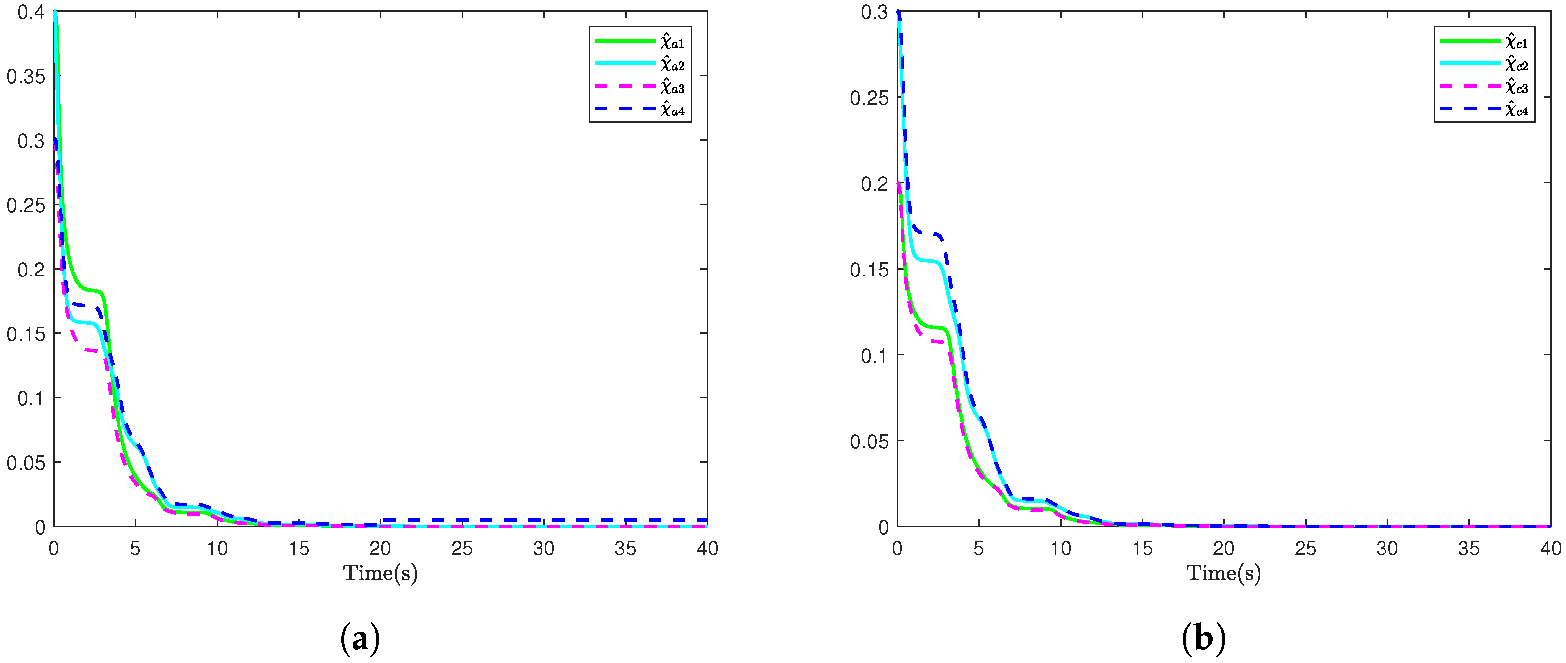
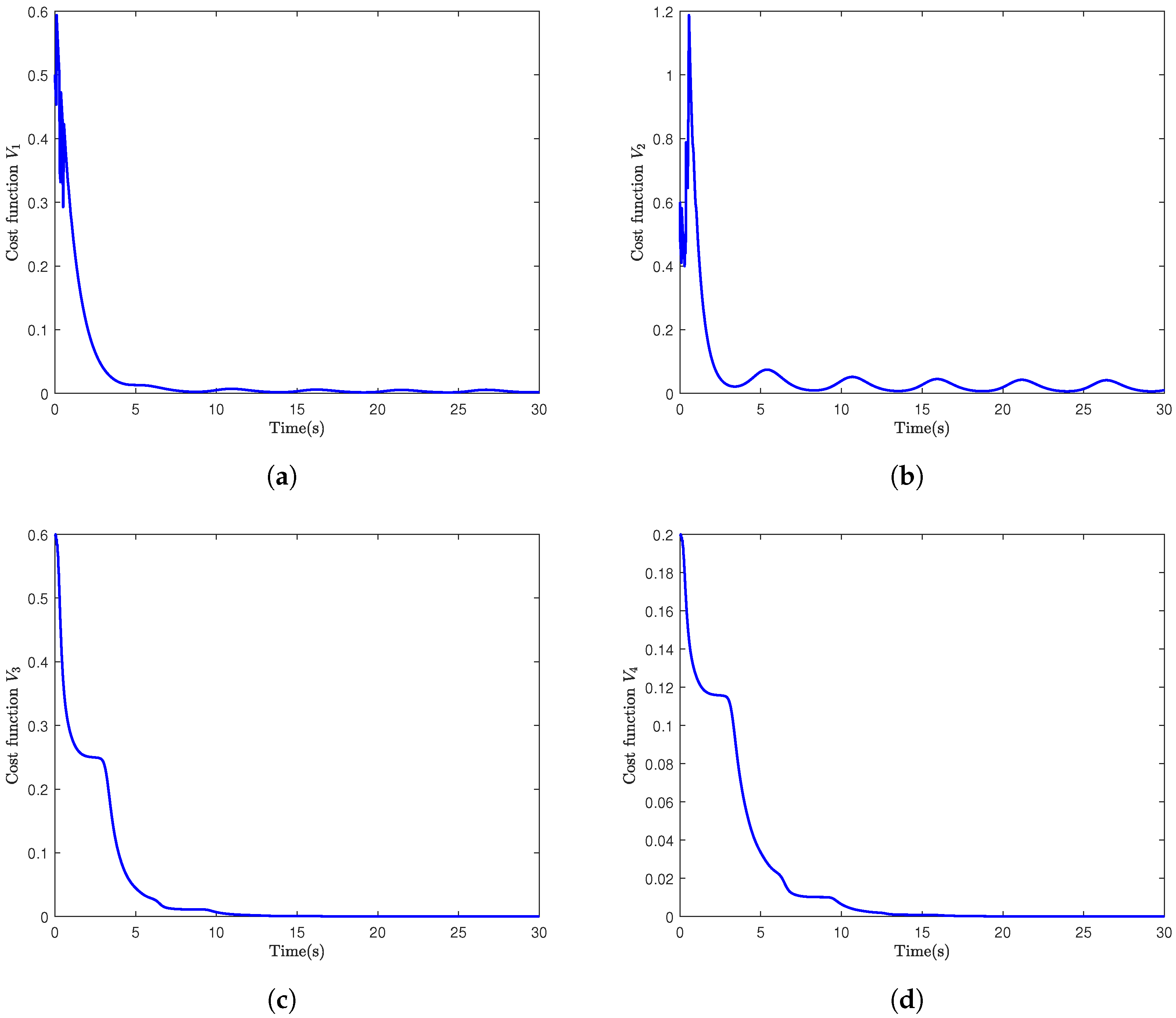
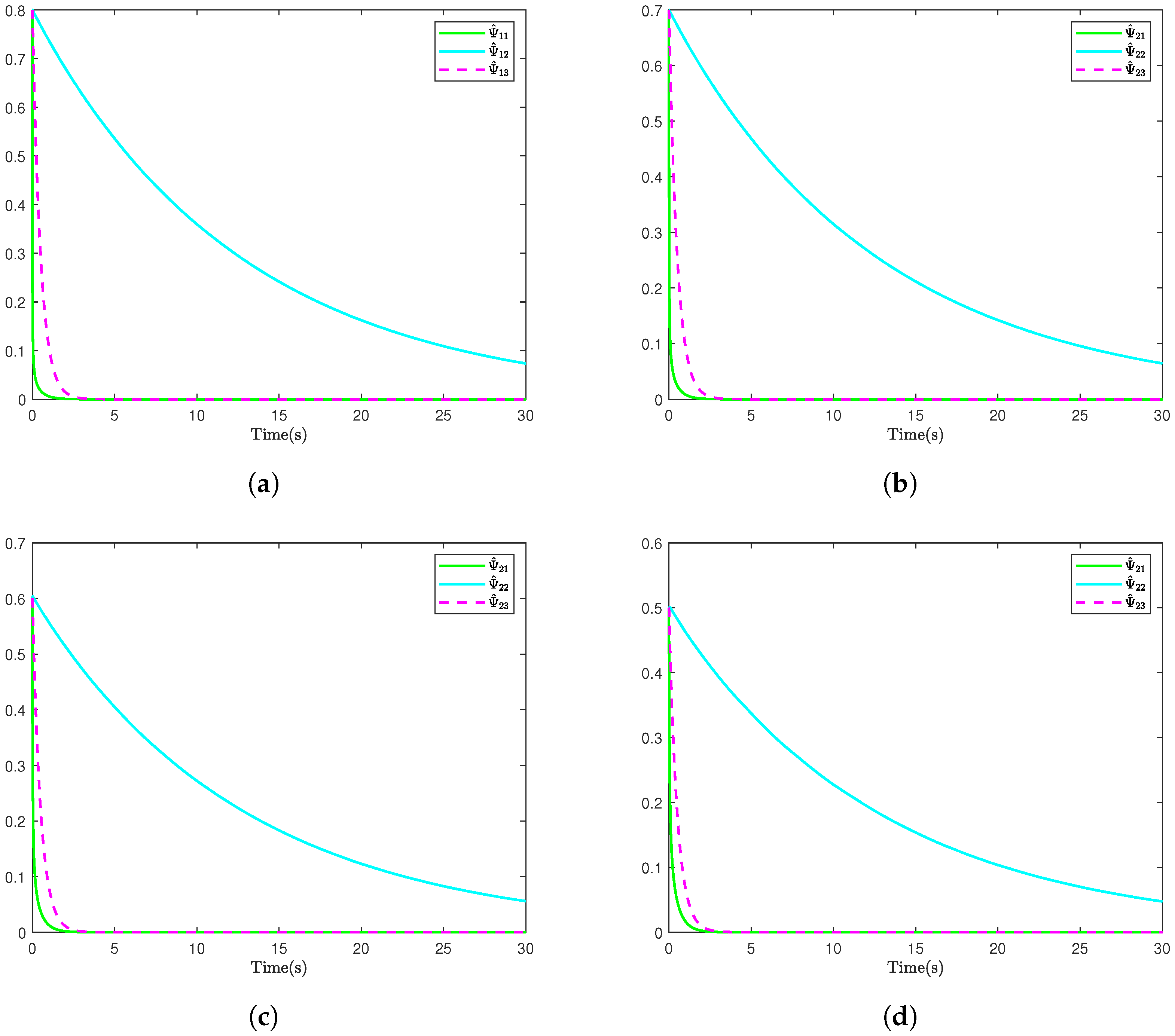
Figure 5 shows the evolution of actor and critic weights, respectively. All weights converge to small steady-state values, which demonstrates stable learning and successful approximation of the optimal control policy. Finally, Figure 6 shows the evolution of the cost functions V 1 , V 2 , and V 3 , offering a quantitative assessment of the optimization objective. The decreasing trends of these functions indicate that the proposed control scheme successfully minimizes the predefined infinite-horizon costs while respecting safety and performance constraints. Figure 7 presents the evolution of the adaptive laws, indicating that the system signals converge to near-zero steady states.

4.3. Sensitivity Analysis of Learning Parameters

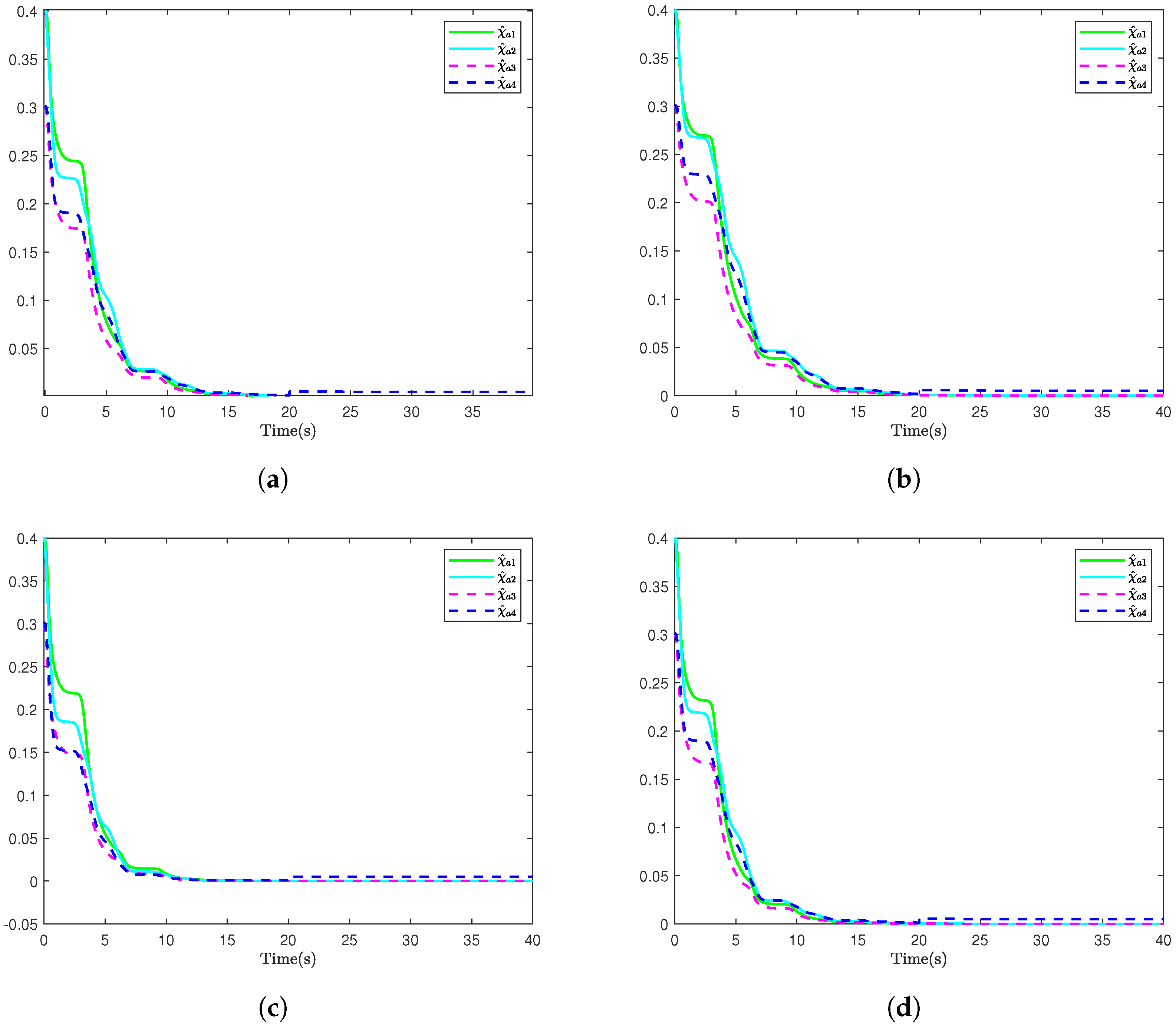
To analyze the influence of the learning gains, a sensitivity study is performed for the actor neural network weights. Table 2 summarizes the sensitivity analysis results of the actor-network learning parameters. Compared with the nominal case, reducing k c i or k a i leads to smoother learning trajectories but slower convergence, whereas increasing k c i or k a i improves the convergence speed at the cost of increased learning oscillations. It is worth noting that all tested cases remain stable, which verifies the robustness of the proposed learning mechanism with respect to moderate parameter variations. Therefore, the learning gains should be selected by considering both convergence speed and closed-loop smoothness. In this work, the nominal parameters k c i = 0.8 and k a i = 1.0 are adopted because they provide a satisfactory balance between fast convergence and low oscillation.
To further investigate the influence of learning gains on the online learning process, a sensitivity analysis is conducted for the actor neural network weights. The nominal learning gains are selected as k c 0 = 0.8 and k a 0 = 1.0 . Based on this nominal setting, different combinations of k c i and k a i are tested while keeping the other simulation parameters unchanged.
Figure 8 illustrates the actor neural network weight trajectories under different learning gain settings. It can be observed that all actor weights remain bounded and eventually converge to a small neighborhood around zero, indicating that the learning process is stable for all tested parameter combinations. Under the nominal setting k c i = 0.8 and k a i = 1.0 , the actor weights exhibit smooth convergence with relatively low oscillation. When k c i is reduced to 0.4 , the convergence becomes slower, and the weights require a longer time to approach the steady-state region. In contrast, increasing k c i to 1.2 or increasing k a i to 1.2 accelerates the convergence of the actor weights, but mild fluctuations and small overshoots appear during the transient stage. These results indicate that larger learning gains can improve the learning speed, while excessively large gains may introduce oscillatory behavior in the weight update process.

4.4. Ablation Study on PPC and RL Components

To further verify the individual contributions of the prescribed performance control and reinforcement learning components, an ablation study is conducted in this subsection. In addition to the proposed complete PPC-RL configuration, two alternative configurations are considered. In the first case, the PPC mechanism is removed while the RL-based optimal learning structure is retained, denoted as the No-PPC configuration. In the second case, the RL component is removed while the PPC mechanism is retained, denoted as the No-RL configuration.
All three configurations are tested under the same initial conditions, desired formation geometry, and simulation parameters, allowing a clear comparison of their tracking performance. The mean square error (MSE), root mean square error (RMSE), and mean absolute error (MAE) are adopted as quantitative performance indices, which are defined as
MSE = 1 n k = 1 n e i 2 , RMSE = 1 n k = 1 n e i 2 , MAE = 1 n k = 1 n | e i | .
The overall comparison results are listed in Table 3.
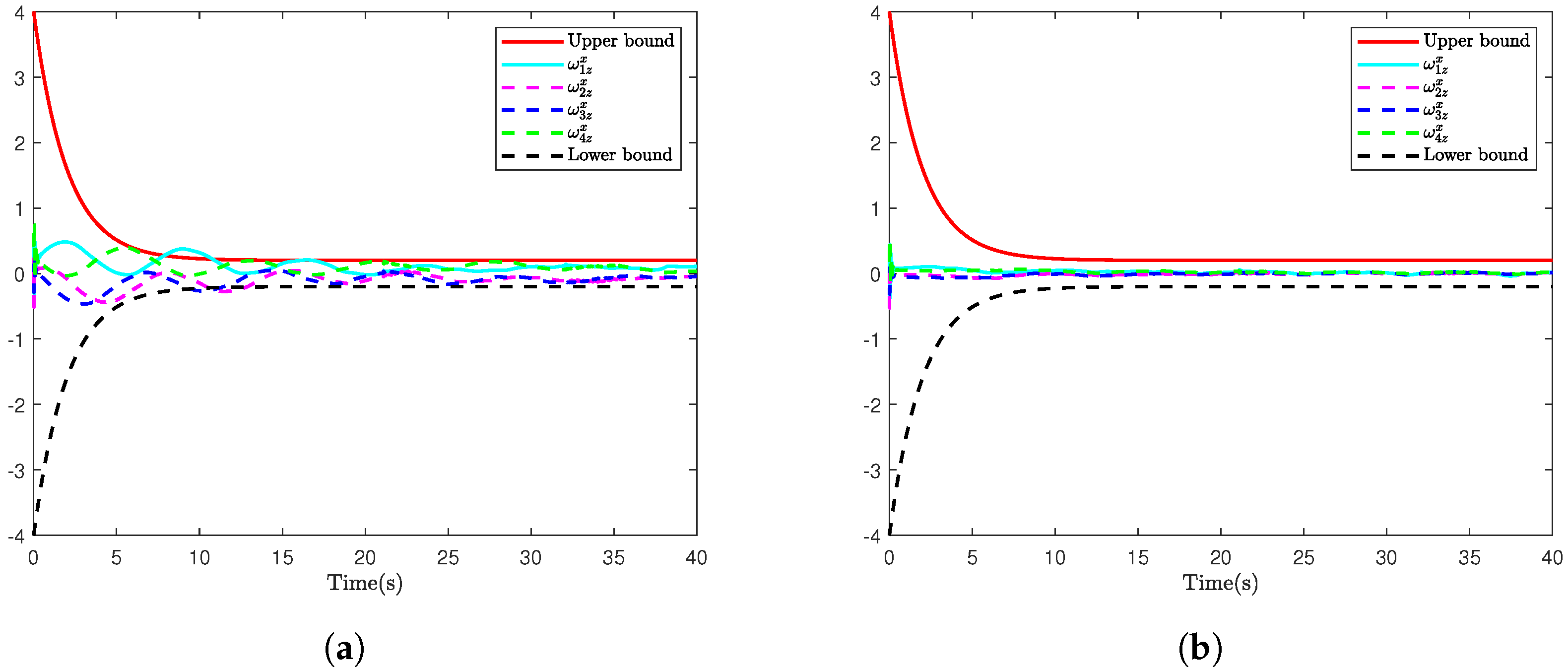
Table 3 shows that the proposed PPC-RL controller achieves the smallest MSE, RMSE, and MAE. Removing PPC significantly degrades tracking performance (RMSE from 0.031613 to 0.173645, MAE from 0.009885 to 0.129873), confirming that PPC is essential for enforcing prescribed error bounds and transient performance. Removing RL also reduces accuracy (RMSE to 0.052556, MAE to 0.028103), verifying that RL enhances optimality. Thus, PPC and RL play complementary roles: PPC guarantees prescribed performance and safety, while RL improves optimal control, and their integration yields the best overall performance.
Figure 9 compares the tracking errors of the PPC-RL, without PPC, and without RL. The proposed method achieves the fastest convergence and smallest steady-state error. The control scheme without PPC shows larger oscillations and poorer transient performance, while the control scheme without RL performs better than No-PPC but still worse than PPC-RL. These results confirm the necessity of integrating both PPC and RL in the framework.
Discussion: Although the proposed framework shows promising simulation results, several practical issues should be further considered before real fixed-wing UAV deployment. First, the current design assumes reliable communication under a fixed topology, while real UAV swarms may experience delays, packet loss, bandwidth limits, and link interruptions. Future work should therefore consider event-triggered communication, delay compensation, and switching topologies. Second, the control commands, including velocity, course angle, and pitch angle, are constrained by actuator saturation, rate limits, and flight envelope restrictions in real UAVs. Thus, input constraints and safety filters should be incorporated. Third, although the simplified actor–critic structure reduces computational burden, its real-time performance on embedded processors should be further tested, especially for large-scale formations. Finally, sensor noise, GPS drift, and estimation delays may affect error transformation and online learning, so robust filtering, sensor fusion, hardware-in-the-loop tests, and flight experiments will be considered in future work.

5. Conclusions

This study has presented formation optimal control scheme for fixed-wing UAV systems by proposing a safe optimal control framework that bridges the gap between performance optimization and safety assurance. By embedding PPC within a simplified actor–critic RL architecture, the proposed method achieved near-optimal control for coupled position–attitude dynamics without reliance on accurate models, thereby significantly enhancing energy efficiency. Simultaneously, the PPC mechanism ensures that all inter-UAV safety distances were strictly preserved. Furthermore, the Lyapunov theory analysis confirmed that all closed-loop signals remain SGUUB and that formation errors consistently stay within predefined boundaries.
Despite promising results, several limitations remain. First, the framework assumes a fixed communication topology, limiting its use in large-scale or dynamic swarms. Second, actor–critic learning is sensitive to initial weights and lacks provable global convergence. Third, structural vibration and material-dependent damping are not explicitly considered. Fourth, only simulation validation has been conducted. Implementation challenges include careful tuning of prescribed performance parameters and the computational load of online neural-network learning on onboard processors. Future work will focus on: (i) scalability to larger formations with dynamic topologies; (ii) resilience against cyberattacks, communication outages, and vibration-induced disturbances; (iii) extension to vibration-aware fixed-wing UAV models; and (iv) experimental flight tests for real-world validation.

Author Contributions

S.Q.: Writing—original, methodology. X.H.: Theoretical guidance. D.S.: Simulation guidance and communication author. All authors have read and agreed to the published version of the manuscript.

Funding

This work was supported by the Fundamental Research Funds for the Central Universities (No. 22120260160).

Data Availability Statement

Data will be made available on request.

Conflicts of Interest

The authors declare no conflicts of interest.

Abbreviations

The following abbreviations are used in this manuscript:
UAVUnmanned Aerial Vehicle
RLReinforcement Learning
PPCPrescribed Performance Control
HJBHamilton–Jacobi–Bellman
RBFNNRadial Basis Function Neural Network
MSEMean Square Error
RMSERoot Mean Square Error
MAEMean Absolute Error

Appendix A

Appendix A.1. RBF Neural-Network

In control engineering, the radial basis function neural network (RBFNN) is widely used for approximating unknown nonlinear functions due to its high accuracy [20]. Consider a continuous function D ( x ¯ i ) : R i n R n with input x ¯ i Ω x ¯ i R i n . The RBFNN approximation is given by
D ( x ¯ i ) = W ϕ ( x ¯ i ) ,
where W R l × n is the weight matrix, l the number of nodes, and ϕ ( x ¯ i ) = [ ϕ 1 ( x ¯ i ) , , ϕ l ( x ¯ i ) ] R l with Gaussian basis functions
ϕ j ( x ¯ i ) = exp x ¯ i c j 2 2 b j 2 , j = 1 , , l ,
where c j R i n and b j R are design parameters.
It is known that any continuous function on a compact set Ω x ¯ i can be approximated with arbitrary accuracy as
D ( x ¯ i ) = W * ϕ ( x ¯ i ) + δ i ( x ¯ i ) ,
with W * R l × n the ideal weight and δ i ( x ¯ i ) the bounded approximation error. There exists a constant δ * > 0 such that δ i < δ * . The ideal weight is defined for analytical purposes as
W * = arg min W R l × n sup x ¯ i Ω x ¯ i D ( x ¯ i ) W ϕ ( x ¯ i ) .

References

  1. Wang, H.; Wang, J.; Ding, G.; Chen, J.; Gao, F.; Han, Z. Completion Time Minimization with Path Planning for Fixed-Wing UAV Communications. IEEE Trans. Wirel. Commun. 2019, 18, 3485–3499. [Google Scholar] [CrossRef]
  2. Huang, Z.; Chen, M.; Shi, P. Disturbance Utilization-Based Tracking Control for the Fixed-Wing UAV with Disturbance Estimation. IEEE Trans. Circuits Syst. Regul. Pap. 2023, 70, 1337–1349. [Google Scholar]
  3. Lv, M.; Ahn, C.K.; Zhang, B.; Fu, A. Fixed-Time Antisaturation Cooperative Control for Networked Fixed-Wing Unmanned Aerial Vehicles Considering Actuator Failures. IEEE Trans. Aerosp. Electron. Syst. 2023, 59, 8812–8825. [Google Scholar] [CrossRef]
  4. Wang, Y.; Shan, M.; Wang, D. Motion Capability Analysis for Multiple Fixed-Wing UAV Formations with Speed and Heading Rate Constraints. IEEE Trans. Control Netw. Syst. 2020, 7, 977–989. [Google Scholar]
  5. Yan, X.; Fang, X.; Deng, C.; Wang, X. Joint Optimization of Resource Allocation and Trajectory Control for Mobile Group Users in Fixed-Wing UAV-Enabled Wireless Network. IEEE Trans. Wirel. Commun. 2024, 23, 1608–1621. [Google Scholar] [CrossRef]
  6. Shi, Y.; Li, J.; Lv, M.; Wang, N. Event-Based Fuzzy Asynchronous Consensus for UAV Swarm Under Jointly Connected Digraphs. IEEE Trans. Fuzzy Syst. 2025, 33, 3195–3209. [Google Scholar] [CrossRef]
  7. Wróbel, J.; Jendryka, K.; Milewski, M.; Kierzkowski, A.; Stosiak, M.; Prentkovskis, O.; Karpenko, M. Experimental Modal Testing of Lightweight Composite UAV Structures: Methods and Key Challenges. Machines 2026, 14, 457. [Google Scholar] [CrossRef]
  8. Karpenko, M.; Stosiak, M.; Deptuła, A.; Urbanowicz, K.; Nugaras, J.; Królczyk, G.; Żak, K. Performance evaluation of extruded polystyrene foam for aerospace engineering applications using frequency analyses. Int. J. Adv. Manuf. Technol. 2023, 126, 5515–5526. [Google Scholar] [CrossRef]
  9. Karpenko, M.; Nugaras, J. Vibration damping characteristics of the cork-based composite material in line to frequency analysis. J. Theor. Appl. Mech. 2022, 60, 593–602. [Google Scholar] [CrossRef] [PubMed]
  10. Meng, B.; Zhang, K.; Jiang, B. Fixed-Time Optimal Fault-Tolerant Formation Control with Prescribed Performance for Fixed-Wing UAVs Under Dual Faults. IEEE Trans. Signal Inf. Process. Over Netw. 2023, 9, 875–887. [Google Scholar] [CrossRef]
  11. Bu, X.; Lv, M.; Lei, H. Discrete-Time Optimal Control Ensuring Fixed-Time Prescribed Performance for SSP. IEEE Trans. Aerosp. Electron. Syst. 2025, 61, 3398–3407. [Google Scholar] [CrossRef]
  12. Zhang, B.; Lv, M.; Cui, S.; Bu, X.; Park, J.H. Learning-Based Optimal Cooperative Formation Tracking Control for Multiple UAVs: A Feedforward-Feedback Design Framework. IEEE Trans. Autom. Sci. Eng. 2025, 22, 11–23. [Google Scholar] [CrossRef]
  13. Yang, Q.; Cao, W.; Meng, W.; Si, J. Reinforcement-Learning-Based Tracking Control of Waste Water Treatment Process Under Realistic System Conditions and Control Performance Requirements. IEEE Trans. Syst. Man Cybern. Syst. 2022, 52, 5284–5294. [Google Scholar] [CrossRef]
  14. Sun, Y.; Xu, J.; Chen, C.; Hu, W. Reinforcement Learning-Based Optimal Tracking Control for Levitation System of Maglev Vehicle with Input Time Delay. IEEE Trans. Instrum. Meas. 2022, 71, 7500813. [Google Scholar] [CrossRef]
  15. Zhou, Y.; Cao, L.; Lei, Y.; Ren, H. Observer-Based Prescribed-Time Optimal Neural Consensus Control for Six-Rotor UAVs: A Novel Actor-Critic Reinforcement Learning Strategy. Neural Netw. 2026, 108644. [Google Scholar] [CrossRef]
  16. Yin, S.; Zhao, S.; Zhao, Y.; Yu, F.R. Intelligent Trajectory Design in UAV-Aided Communications with Reinforcement Learning. IEEE Trans. Veh. Technol. 2019, 68, 8227–8231. [Google Scholar] [CrossRef]
  17. Cui, J.; Liu, Y.; Nallanathan, A. Multi-Agent Reinforcement Learning-Based Resource Allocation for UAV Networks. IEEE Trans. Wirel. Commun. 2020, 19, 729–743. [Google Scholar] [CrossRef]
  18. Lv, M.; De Schutter, B.; Shi, C.; Baldi, S. Logic-based distributed switching control for agents in power-chained form with multiple unknown control directions. Automatica 2022, 137, 110143. [Google Scholar] [CrossRef]
  19. Wen, G.; Chen, C.P.; Li, B. Optimized formation control using simplified reinforcement learning for a class of multiagent systems with unknown dynamics. IEEE Trans. Ind. Electron. 2020, 67, 7879–7888. [Google Scholar] [CrossRef]
  20. Wen, G.; Ge, S.S.; Tu, F. Optimized backstepping for tracking control of strict-feedback systems. IEEE Trans. Neural Netw. Learn. Syst. 2018, 29, 3850–3862. [Google Scholar] [CrossRef]
  21. Wen, G.; Chen, C.P.; Ge, S.S. Simplified optimized backstepping control for a class of nonlinear strict-feedback systems with unknown dynamic functions. IEEE Trans. Cybern. 2021, 51, 4567–4580. [Google Scholar] [CrossRef]
  22. Hamidoğlu, A. Designing discrete-time control-based strategies for pursuit-evasion games on the plane. Optimization 2025, 74, 239–268. [Google Scholar] [CrossRef]
  23. Hamidoğlu, A.; Gul, O.M.; Kadry, S.N.; Jana, C.; Elghirani, A.; Gultekin, G.K. A cost-effective nash-based allocation method for task distribution of multiple robots in distributed robotic networks. Eng. Appl. Artif. Intell. 2025, 162, 112548. [Google Scholar] [CrossRef]
  24. Lv, M.; Chen, Z.; De Schutter, B.; Baldi, S. Prescribed-performance tracking for high-power nonlinear dynamics with time-varying unknown control coefficients. Automatica 2022, 146, 110584. [Google Scholar] [CrossRef]
  25. Tian, G.; Golestani, M.; Lam, J.; Duan, G.; Kong, H. Prescribed-Time Control of Nonlinear Systems with Global Prescribed Performance for State Errors. IEEE Trans. Circuits Syst. Regul. Pap. 2025, 72, 6148–6158. [Google Scholar] [CrossRef]
  26. Wang, P.; Yu, C.; Lv, M. Optimized Formation Control of Nonlinear Systems with Full-State Constraints Using Adaptive Fixed-Time Techniques. IEEE Trans. Autom. Sci. Eng. 2025, 22, 3331–3344. [Google Scholar] [CrossRef]
  27. Lv, M.; Wang, N. Distributed Control for Uncertain Multiagent Systems with the Powers of Positive-Odd Numbers: A Low-Complexity Design Approach. IEEE Trans. Autom. Control 2024, 69, 434–441. [Google Scholar] [CrossRef]
  28. Zhang, G.; Xing, Y.; Zhang, W.; Li, J. Prescribed Performance Control for USV-UAV via a Robust Bounded Compensating Technique. IEEE Trans. Control Netw. Syst. 2025, 12, 2289–2299. [Google Scholar] [CrossRef]
  29. Yang, S.; Zhao, Z.; Zhu, X.; Huang, Y.; Zhang, W. Adaptive Robust Constraint-Following Control with Prescribed Performance for Quadrotor UAV Subjected to Time-Varying Uncertainties. IEEE Trans. Transp. Electrif. 2026, 12, 1630–1641. [Google Scholar] [CrossRef]
  30. Lv, M.; De Schutter, B.; Cao, J.; Baldi, S. Adaptive Prescribed Performance Asymptotic Tracking for High-Order Odd-Rational-Power Nonlinear Systems. IEEE Trans. Autom. Control 2023, 68, 1047–1053. [Google Scholar] [CrossRef]
  31. Wang, Y.; Wang, H.; Liu, Y.; Li, J. Neural Adaptive Coordinated Docking Control with Improved Prescribed Performance for UAV Aerial Recovery. IEEE Trans. Ind. Electron. 2024, 71, 16546–16557. [Google Scholar] [CrossRef]
  32. Bu, X. Saturated Control with Variable Prescribed Performance Applied to the Manipulator of UAV. IEEE J. Miniaturization Air Space Syst. 2023, 4, 212–220. [Google Scholar] [CrossRef]
  33. Wang, X.; Baldi, S.; Feng, X.; Wu, C.; Xie, H.; De Schutter, B. A Fixed-Wing UAV Formation Algorithm Based on Vector Field Guidance. IEEE Trans. Autom. Sci. Eng. 2023, 20, 179–192. [Google Scholar] [CrossRef]
  34. Shi, Y.; Li, J.; Lv, M.; Wang, N.; Zhang, B. Distributed Consensus Control for 6-DOF Fixed-Wing Multi-UAVs in Asynchronously Switching Topologies. IEEE Trans. Veh. Technol. 2025, 74, 5649–5663. [Google Scholar] [CrossRef]
  35. Yang, X.; Huang, C.; Cao, J.; Liu, H. Predefined-time adaptive fuzzy echo state network containment control of uncertain multiagent systems with prescribed performance. Expert Syst. Appl. 2025, 286, 128046. [Google Scholar] [CrossRef]
  36. Deng, C.; Yang, G. Distributed adaptive fuzzy control for nonlinear multiagent systems under directed graphs. IEEE Trans. Fuzzy Syst. 2018, 26, 1356–1366. [Google Scholar]
  37. Wang, M.; Liang, H.; Pan, Y.; Xie, X. A New Privacy Preservation Mechanism and a Gain Iterative Disturbance Observer for Multiagent Systems. IEEE Trans. Netw. Sci. Eng. 2023, 11, 392–403. [Google Scholar] [CrossRef]
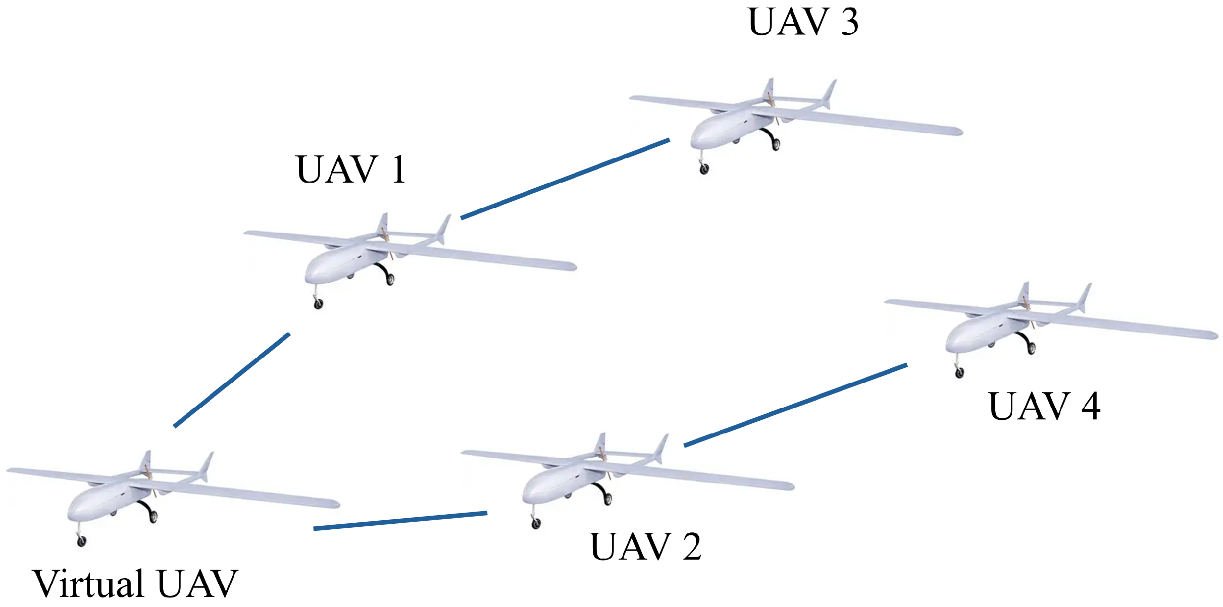
Figure 1. Communication relationship.
Machines 14 00583 g001
Figure 2. 3D formation scenarios showed by Tacview: (a) Formation configuration scenario. (b) Formation keeping scenario.
Machines 14 00583 g002
Figure 3. State errors of UAVs: (a) Error on x axis. (b) Error on y axis. (c) Error on z axis. (d) Error on z axis without prescribed performance control.
Machines 14 00583 g003
Figure 4. Attitude errors of UAVs: (a) Error on velocity. (b) Error on course angle. (c) Error on pitch angle. (d) Error on pitch angle without prescribed performance control.
Machines 14 00583 g004
Figure 5. Curves of actor and critic weights: (a) Actor weights of UAV. (b) Critic weights of UAV.
Machines 14 00583 g005
Figure 6. Cost function: (a) Cost function V 1 . (b) Cost function V 2 . (c) Cost function V 3 . (d) Cost function V 4 .
Machines 14 00583 g006
Figure 7. Adaptive laws: (a) Adaptive laws of UAV 1. (b) Adaptive laws of UAV 2. (c) Adaptive laws of UAV 3. (d) Adaptive laws of UAV 4.
Machines 14 00583 g007
Figure 8. Actor neural network weight trajectories under different learning parameters: (a) k c i = 0.8 , k a i = 1.0 ; (b) k c i = 0.4 , k a i = 1.0 ; (c) k c i = 1.2 , k a i = 1.0 ; (d) k c i = 0.8 , k a i = 1.2 .
Machines 14 00583 g008
Figure 9. Curves of quantitative comparison: (a) Without prescribed performance control. (b) Without reinforcement learning.
Machines 14 00583 g009
Table 1. Summary of existing control approaches.
Method CategoryMain AdvantageMain LimitationDifference of This Work
Robust/adaptive UAV controlHandles uncertainties and disturbancesUsually does not optimize long-term control costIntroduces actor–critic RL to approximate optimal control
Conventional actor–critic UAV controlLearns near-optimal policy under limited model knowledgeSafety constraints are not explicitly guaranteedUses PPC to enforce formation error bounds
PPC-based UAV controlGuarantees transient/steady-state error constraintsOften lacks optimality or energy-efficiency designCombines PPC with HJB-based actor-critic learning
Existing RL-PPC controlCombines learning and performance constraintsOften for single UAV, simplified dynamics, or nonlinear systemsFocuses on UAV formation with coupled position–attitude dynamics
Proposed methodSafe and near-optimal formation controlCurrent validation is simulation-basedEnsures SGUUB stability and defined boundary satisfaction
Table 2. Sensitivity analysis of actor network learning parameters.
Case k ci k ai Convergence TimeLearning OscillationStability
Actor
network
0.8111.7Low
0.4117.0Low
1.218.8Medium
0.81.213.0Medium
Table 3. Quantitative comparison of the proposed controller and ablation cases.
Data TypeMSERMSEMAE
Proposed PPC-RL0.0009990.0316130.009885
Without PPC0.0301530.1736450.129873
Without RL0.0027620.0525560.028103
Disclaimer/Publisher’s Note: The statements, opinions and data contained in all publications are solely those of the individual author(s) and contributor(s) and not of MDPI and/or the editor(s). MDPI and/or the editor(s) disclaim responsibility for any injury to people or property resulting from any ideas, methods, instructions or products referred to in the content.