Longitudinal Finite-Time Control of Intelligent Vehicle Fleet Considering Time-Delay and Interference

Abstract

To address the robustness degradation of intelligent vehicle fleet longitudinal control systems caused by the coexistence of disturbances and time-delay, a longitudinal finite-time control strategy based on a predictive finite-time extended state observer (PFTESO) is proposed. First, a finite-time extended state observer (FTESO) is designed to estimate system disturbances. To address the observer input asynchrony induced by time-delay, an improved Smith predictor is integrated into the FTESO to construct the PFTESO, thereby improving disturbance observation accuracy under delayed conditions. Meanwhile, a proportional–integral (PI) compensation controller is introduced based on the estimation error to further enhance control accuracy. Subsequently, a global fast integral terminal sliding mode controller (GFITSMC) is developed based on the PFTESO to improve the robustness and finite-time convergence performance of the intelligent vehicle fleet system under disturbances and time-delay. Finally, comparative simulation studies under different operating conditions are conducted to evaluate the effectiveness of the proposed strategy. Simulation results demonstrate that the proposed PFTESO effectively improves state observation accuracy under delayed conditions, where the RMSE values of z₁ and z₂ are reduced from 0.082 and 0.214 to 0.021 and 0.067, respectively. In addition, compared with conventional sliding mode control strategies, the proposed FTESO-GFITSMC reduces the peak acceleration chattering from ±0.23 m/s² to 0.03 m/s² while achieving a finite-time convergence time of 13 s. The proposed method exhibits superior robustness, faster convergence performance, and smoother acceleration response for an intelligent vehicle fleet under disturbances and delayed conditions.

1. Introduction

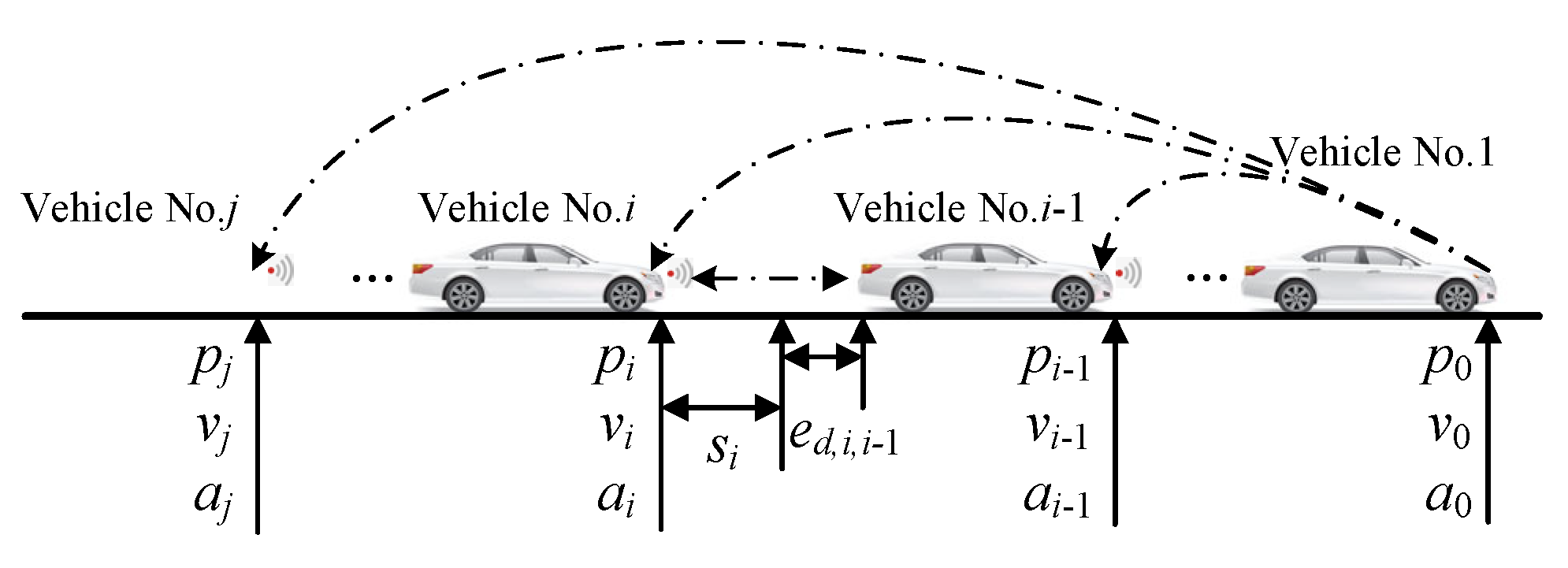
In the complex urban road network, intelligent transportation systems have been developed to improve traffic conditions and driving safety [1,2]. An intelligent vehicle fleet is one of the most important technologies of intelligent transportation systems, holding substantial promise for cultivating ecologically sustainable transportation networks [3]. An intelligent vehicle fleet is a vehicle queue composed of multiple intelligent vehicles that can communicate with each other. Vehicles in the queue can obtain the state information of other vehicles through onboard sensors and communication devices and dynamically adjust the optimal distance to realize safe driving of the fleet and improve traffic efficiency [4].

Adaptive cruising with minimal safe inter-vehicle spacing, while concurrently ensuring fleet stability, is a pivotal challenge in vehicle fleet control [5]. A wealth of advanced control algorithms have been proposed as prospective solutions to address this critical issue, such as model predictive control [6,7], neural network control [8], sliding mode control [9], and robust control [10]. Mosharafian et al. addressed the multifaceted challenges in the safety control of intelligent vehicle fleets and smooth traffic flow by constructing a hybrid model predictive control strategy operating under three distinct modes: free following, warning, and emergency braking [11]. In light of the intricate uncertainties and nonlinear behaviors exhibited by intelligent vehicle fleet systems, Guo introduced a hierarchical control framework composed of an upper-layer model predictive controller and a lower-layer adaptive neural network sliding mode controller (ANN-SMC) [12]. In the upper layer, the model predictive controller was employed to generate smooth desired acceleration commands in real time, while saturation characteristics were introduced to constrain the acceleration within a predefined range. In the lower layer, the uncertainties and variable structure control terms were adaptively adjusted by the neural network, and the stability of the proposed ANN-SMC was guaranteed using the Lyapunov theory. Molnár et al. investigated vehicle fleet dynamics and proposed two robust control strategies in which the feedback gain was regulated to address parameter perturbations within the control loop [13].

Notably, most existing control algorithms mainly focus on improving vehicle dynamic performance, such as vehicle speed tracking and acceleration smoothness. However, the convergence performance of the spacing error remains a crucial issue in vehicle fleet control systems. The convergence speed directly affects fleet efficiency, driving safety, and disturbance recovery capability [14,15]. Existing methodologies have mainly synthesized vehicle fleet controllers based on the Lyapunov asymptotic stability theory, which cannot explicitly guarantee optimal control performance in the time domain [16]. Recent studies have demonstrated that, compared with asymptotically stable control systems, finite-time closed-loop control systems can achieve better robustness and stronger anti-interference capability [17,18]. Therefore, developing a longitudinal cooperative control system for an intelligent vehicle fleet based on finite-time control methodologies is of great significance, especially under complex driving conditions.

The longitudinal driving stability of a vehicle fleet is greatly affected by numerous external factors, such as rolling resistance variations caused by changes in road adhesion coefficients and measurement noise introduced by onboard sensors. In particular, sensor measurement noise, as a kind of mismatched disturbance, is usually imposed on the controller input side and significantly affects control performance. However, finite-time stability analysis of intelligent vehicle systems under mismatched disturbances has been rarely investigated in existing studies, with most research primarily focusing on the effects of matched disturbances. To address parameter uncertainty within vehicle fleet systems, Chehardoli adopted the recursive least squares method to identify the parameters governing longitudinal vehicle dynamics and subsequently designed a linear robust controller to achieve stable control of relative vehicle spacing and velocity [19]. By combining the integral sliding mode method with the finite-time Lyapunov theory, Coppola et al. introduced a distributed finite-time control strategy characterized by rapid convergence of vehicle spacing within a predefined time interval under external disturbances regardless of initial conditions [20]. Considering the influence of model uncertainty and external disturbances, Aghababa et al. proposed a robust terminal sliding mode controller based on a novel spacing error definition, which ensured finite-time rapid convergence of vehicle spacing as well as global stability of the vehicle fleet [21].

It is worth noting that, although considerable progress has been achieved in improving the robustness of vehicle fleet systems under external disturbances, the impact of the coexistence of time-delay and disturbances on vehicle fleet robustness remains largely unexplored in existing studies. In practical vehicle fleet systems, communication delay, controller computation delay, actuator response delay, and sensor transmission delay are unavoidable [22,23]. When time-delay and mismatched disturbances coexist, the time-delay may lead to asynchronous observer inputs, causing the system states and control inputs received by the observer to become temporally inconsistent. This asynchrony degrades disturbance observation accuracy, weakens system robustness, and further affects the finite-time convergence performance of vehicle fleet systems.

In light of the aforementioned research gaps, this paper elaborates on the construction of a finite-time extended state observer (FTESO) tailored to address system mismatched disturbances. An improved Smith predictor is introduced into the FTESO to construct a predictive finite-time extended state observer (PFTESO), thereby alleviating the influence of time-delay on the state observer and improving disturbance observation accuracy under delayed conditions. On this basis, and from the perspective of finite-time optimal control, a global fast integral terminal sliding mode controller (GFITSMC) is further designed by combining finite-time theory with predicted state observation results to improve the driving performance and robustness of intelligent vehicle fleet systems under time-delay and disturbances. The main contributions of this study are summarized as follows:

(1)

In order to address the limitation that intelligent vehicle fleet systems cannot achieve time-optimal control based on infinite-time asymptotic stability theory, the GFITSMC is proposed to improve the convergence performance of vehicle spacing errors. Meanwhile, a nonsmooth reaching law (NSRL) is constructed to ensure that the vehicle spacing error reaches the sliding mode surface within finite-time while effectively suppressing the chattering phenomenon caused by the discontinuity of the conventional sign function.

(2)

The influences of time-delay and disturbances on the stability of the intelligent vehicle fleet is comprehensively considered. An improved Smith predictor is introduced into the FTESO to alleviate the asynchronous observer input problem caused by time-delay. Based on the predicted extended state observation results, a finite-time controller is designed to improve fleet robustness and convergence performance under the coexistence of time-delay and disturbances.

The remainder of this paper is organized as follows. Section 2 introduces the control problem of the intelligent vehicle fleet and preliminary knowledge. Section 3 presents the controller design and stability analysis. Section 4 provides comparative simulation studies under different scenarios. Finally, the conclusions are drawn in Section 5.

2. Problem Description and Preliminary Knowledge

2.1. Problem Description

The longitudinal intelligent vehicle fleet considered in this study is shown in Figure 1. The fleet consists of multiple intelligent vehicles traveling along a straight road, where p_i, v_i, and a_i represent the longitudinal position, velocity, and acceleration of the i-th vehicle (i = 0,1,2,3…), respectively. The variable s_i denotes the desired safe inter-vehicle spacing, while e_d,i,j represents the vehicle spacing error between the i-th and j-th vehicles.

In intelligent vehicle fleet systems, vehicles exchange motion information through onboard sensors and vehicle-to-vehicle (V2V) communication devices to maintain safe spacing and coordinated longitudinal motion. According to different communication architectures, the fleet communication topology can generally be classified into two types. If the vehicles in the fleet can directly obtain the leading vehicle information through V2V communication, the communication structure is referred to as the Lead–Follow (LF) topology. Alternatively, if each vehicle can only obtain the motion information of its preceding vehicle through onboard sensors, the communication structure is defined as the Preceding–Follow (PF) topology.

The lateral dynamics of the intelligent vehicle fleet are ignored in this study, and only the longitudinal driving dynamics under external disturbances are considered. The vehicle spacing strategy between adjacent vehicles can be described as

$$d_{i,j}=p_j-p_i-h_i\left(j-i\right){\dot{p}}_i-l_i\left(j-i\right),$$

(1)

where h_i is the vehicle spacing coefficient and the value is 1~2; l_i is the body length of the ith vehicle; and d_i,j is the relative spacing between the ith and jth vehicles.

The longitudinal dynamics of the vehicle fleet can be expressed as the following nonlinear model:

$$\begin{array}{l}{\dot{e}}_{d,i,j}={\dot{p}}_j-{\dot{p}}_i-h_i\left({\dot{v}}_i+{\dot{d}}_i\right),\\ {\dot{e}}_{v,i,j}=a_i-a_j,\\ {\dot{a}}_i=-{\displaystyle \frac{1}{{\tau }_i}}{a}_i+{\displaystyle \frac{1}{m_i{\tau }_i}}\left[{\displaystyle \frac{i_g{i}_0{\eta }_t{T}_{e,i}}{r_{w,i}}}-F_i\right].\end{array}$$

(2)

where d_i denotes the measurement noise of the vehicle speed sensor, which is modeled as a mismatched disturbance acting on the controller input channel; τ_i is the engine response coefficient; m_i is the vehicle body mass; i_g and i₀ are ratios of the transmission and main reducer, respectively; η_t is the mechanical efficiency; r_w,i is the wheel radius; T_e,i is the engine torque; and F_i is the vehicle driving resistance.

In practical intelligent vehicle fleet systems, communication delay, controller computation delay, actuator response delay, and sensor transmission delay are unavoidable. When the system is simultaneously affected by sensor measurement noise and time-delay, the observer inputs may become temporally asynchronous, thereby degrading disturbance observation accuracy and affecting the robustness and convergence performance of the fleet control system. Therefore, both mismatched disturbances and time-delay are comprehensively considered in this study.

Assuming that the target vehicle is driving at the desired acceleration a_dmd, the expected output torque of the engine can be expressed as

$$T_{e,i}={\displaystyle \frac{1}{i_g{i}_0{\eta }_t}}\left[F_i+m_i{a}_{\mathrm{dmd}}\right]r_{w,i},$$

(3)

The longitudinal nonlinear model of the fleet can be further rewritten as

$$\begin{array}{l}{\dot{e}}_{d,i,j}={\dot{p}}_j-{\dot{p}}_i-h_i\left({\dot{v}}_i+{\dot{d}}_i\right),\\ {\dot{e}}_{v,i,j}=a_i-a_j,\\ {\dot{a}}_i=-{\displaystyle \frac{1}{{\tau }_i}}{a}_i+{\displaystyle \frac{1}{{\tau }_i}}{u}_i.\end{array}$$

(4)

where u_i = a_dmd is the control input of the i-th vehicle.

2.2. Preliminary Knowledge

To facilitate the subsequent finite-time stability analysis of the predictive finite-time extended state observer (PFTESO) and the global fast integral terminal sliding mode controller (GFITSMC), the following finite-time stability theorems and string stability lemmas are introduced:

Theorem 1

([24]). For the following system,

$$\dot{x}\left(t\right)=f\left(x\left(t\right)\right),$$

(5)

if there is a continuously differentiable function V(x) that satisfies

$$\dot{V}\left(x\right)+c{V}^{\alpha }\left(x\right)\le 0,$$

(6)

then the system described by Equation (5) is finite-time stable. The stability time satisfies

$$t\le {\displaystyle \frac{1}{c\left(1-\alpha \right)}}{V}^{1-\alpha }\left(x_0\right).$$

(7)

where the parameters c > 0, 0 < α < 1, and V(x₀) represent the initial value of V(x).

Theorem 2

([25]). Considering the system as shown by Equation (8),

$$\dot{x}\left(t\right)=f\left(x\left(t\right)\right)+d\left(t\right),$$

(8)

if there exists a continuous and first-order differentiable positive function V(x) that satisfies

$$\dot{V}\left(x\right)\le -{\phi }_{1}V{\left(x\right)}^{\gamma }-{\phi }_{2}V\left(x\right)+{\phi }_3,x\in D/\left\{0\right\},$$

(9)

then the system described by Equation (8) is finite-time stable. The system stability time satisfies

$$t\le \max \left\{\begin{array}{l}{\displaystyle \frac{\ln \frac{k{\theta }_0{V}^{1-\gamma }\left(x_0\right)+{\phi }_1}{{\phi }_1}}{k{\theta }_0\left(1-\gamma \right)}},\\ {\displaystyle \frac{\ln \frac{k{V}^{1-\gamma }\left(x_0\right)+{\theta }_0{\phi }_1}{{\phi }_1}}{k\left(1-\gamma \right)}}\end{array}\right\}.$$

(10)

where φ_i > 0, 0 < γ < 1, k > 0, and θ₀ > 0.

Lemma 1

([26]). When the unknown external disturbance D_i is bounded and nonzero and the following inequality (11) is satisfied,

$${{\displaystyle {\int }_0^{T_s}{‖e_{d,i,j}‖}^{2}dt\le {\gamma }_d^2{\displaystyle {\int }_0^{T_s}‖D_i‖}}}^{2}dt.$$

(11)

the nonlinear system described by Equation (4) has strong robustness against disturbances, where γ_d is a robust gain coefficient and satisfies 0 < γ_d < 1.

Lemma 2

([27]). When a vehicle is traveling in a fleet, if the control error of the preceding vehicle will not affect that of the rear vehicle, and will not be transmitted backward along the direction of the fleet, the fleet is stable. Generally, the string stability of a vehicle fleet can be defined as the vehicle spacing error ratio of two adjacent vehicles, as shown by

$$G\left(s\right)={\displaystyle \frac{E_{i+1}\left(s\right)}{E_i\left(s\right)}}.$$

(12)

where E_i(s) is the Laplace transform of the vehicle spacing error between the ith vehicle and its preceding vehicle. When G(s) meets 0 < |G(s)| < 1, the vehicle spacing error will attenuate and converge, and the vehicle satisfies strong string stability.

3. Controller Design and Analysis

During the operation of intelligent vehicle fleet systems, external factors such as vehicle speed measurement noise and communication delay are unavoidable, which may degrade the robustness and convergence performance of the fleet control system. In practical intelligent vehicle fleet systems, mismatched disturbances and time-delay usually coexist simultaneously. When the observer is directly constructed based on delayed measurement signals, the observer inputs may become temporally asynchronous, thereby reducing disturbance observation accuracy and affecting the control performance of the fleet system.

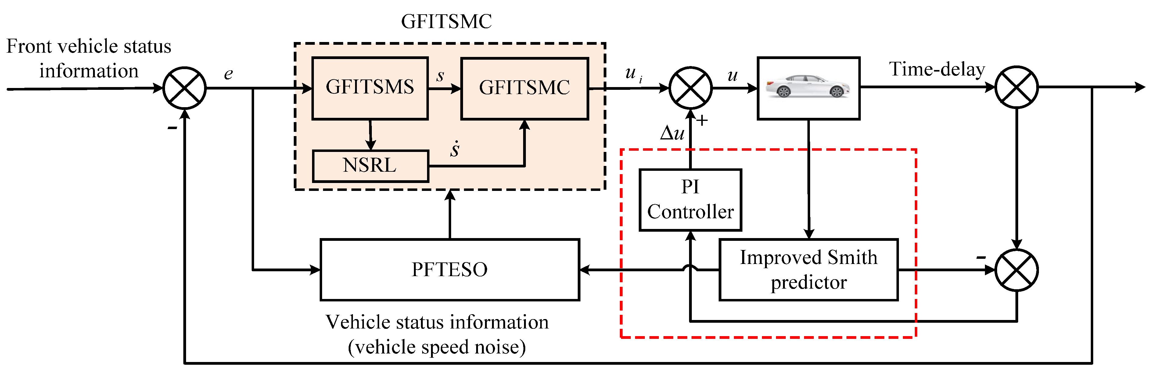
The intelligent vehicle fleet generally adopts a hierarchical control architecture, in which the upper-level controller calculates the desired acceleration and the lower-level controller converts the desired acceleration into actuator commands, including throttle and brake signals. To achieve finite-time longitudinal cooperative control under disturbances and time-delay, the intelligent vehicle fleet control framework shown in Figure 2 is established. The intelligent vehicles obtain state information through onboard sensors and wireless communication devices. A finite-time extended state observer (FTESO) is designed to estimate the vehicle speed measurement noise and lumped disturbances. Meanwhile, an improved Smith predictor is introduced into the FTESO to construct the predictive finite-time extended state observer (PFTESO), thereby alleviating the asynchronous observer input problem caused by time-delay. Based on the predictive state observation results of the PFTESO, a global fast integral terminal sliding mode controller (GFITSMC) is further designed to improve the convergence performance and robustness of the intelligent vehicle fleet system. In addition, a proportional–integral (PI) compensation controller is introduced based on the estimated errors to further improve the control accuracy of the vehicle fleet.

3.1. Upper-Level Controller

3.1.1. Design of the Finite-Time Extended State Observer

The longitudinal error model of the intelligent vehicle fleet under measurement noise disturbance is shown by Equation (4). In this study, the vehicle speed measurement noise is modeled as a mismatched disturbance acting on the controller input channel. To facilitate the observer design and disturbance estimation, the following state variables are defined as

$$\left\{\begin{array}{l}{z}_1=e_{d,i,j}\\ z_2=e_{v,i,j}-h_i{a}_i+h_i{\dot{d}}_i\\ z_3=-\left(1+b\right)a_i+a_j+h_i{\ddot{d}}_i\end{array}\right.,$$

(13)

where b is the system parameter. The longitudinal error model can be rewritten as

$$\left\{\begin{array}{l}{\dot{z}}_1=z_2\\ {\dot{z}}_2=b{u}_i+z_3\end{array}\right.,$$

(14)

To achieve rapid estimation of the system states and lumped disturbances, the finite-time extended state observer (FTESO) is designed as

$$\left\{\begin{array}{l}{\dot{\widehat{z}}}_1={\widehat{z}}_2+L_1{\left({\widehat{z}}_1-z_1\right)}^{m_1}\\ {\dot{\widehat{z}}}_2=b{u}_i+{\widehat{z}}_3+L_2{\left({\widehat{z}}_1-z_1\right)}^{m_2}\\ {\dot{\widehat{z}}}_3=L_3{\left({\widehat{z}}_1-z_1\right)}^{m_3}\end{array}\right..$$

(15)

where L_i (i = 1,2,3) is the observer coefficient; and m_i is the power coefficient (0 < m_i < 1).

The nonlinear correction terms are introduced to ensure finite-time convergence of the observer estimation errors. By properly selecting the observer coefficients, the FTESO can rapidly estimate the vehicle spacing states and lumped disturbances under mismatched disturbance conditions. The stability of the designed finite-time extended state observer is proved in Appendix A.

3.1.2. Design of Predictive Finite-Time Extended State Observer

System time-delay may lead to asynchronous observer inputs, thereby degrading disturbance observation accuracy and weakening the robustness of intelligent vehicle fleet systems. Therefore, predicting and compensating for system time-delay is essential to obtain delay-compensated state information for the observer. Considering that the Smith predictive compensation control is an effective method to overcome pure hysteresis [26], an improved Smith predictor combined with a linear state observer is constructed to estimate the delayed system states and alleviate the asynchronous observer input problem caused by time-delay. The dynamic equation of the i-th vehicle in the system can be expressed as

$$\left\{\begin{array}{l}{\dot{p}}_i\left(t\right)=v_i\left(t\right)\\ {\dot{v}}_i\left(t\right)=a_i\left(t\right)\\ {\dot{a}}_i\left(t\right)=-{\displaystyle \raisebox{1ex}{$1$}\!\left/ \!\raisebox{-1ex}{$\tau $}\right.}{a}_i\left(t\right)+{\displaystyle \raisebox{1ex}{$1$}\!\left/ \!\raisebox{-1ex}{$\tau $}\right.}{u}_i\left(t\right)\end{array}\right.,$$

(16)

Therefore, the state space expression of the vehicle with time-delay can be written as

$$\left\{\begin{array}{l}\dot{x}\left(t-\tau \right)=Ax\left(t-\tau \right)+B{u}_i\left(t-\tau \right)\\ y\left(t\right)=Cx\left(t-\tau \right)\end{array}\right.,$$

(17)

The state vector is

$$x\left(t-\tau \right)={\left[p_i(t-\tau ),v_i(t-\tau ),a_i(t-\tau )\right]}^T,$$

(18)

where p_i(t − τ), v_i(t − τ), and a_i(t − τ) indicate the position, speed, and acceleration of the vehicle at time (t − τ), with τ as the lag time and y(t) is the system output.

The delayed system states are estimated by introducing a linear predictive observer, in which the delayed outputs are utilized to reconstruct synchronized state information. The linear state observer is constructed as

$$\left\{\begin{array}{l}\dot{z}(t)=Az(t)+Bu(t)+L\left[Cz(t)-w(t)\right]\\ \dot{w}(t)=CAz(t)+CBu(t)\\ y(t)=w(t)\end{array}\right.,$$

(19)

where z(t) and w(t) represent the observed states of x(t − τ) and y(t), respectively, and L is the observer parameter matrix.

By defining the state observation error as e₁ = z(t) − x(t − τ), e₂ = y(t) − w(t), according to Equations (17) and (19), the error dynamics can be further formulated as

$$\left\{\begin{array}{l}{\dot{e}}_1=\dot{z}(t)-\dot{x}(t-\tau )\\ = Az(t)+Bu(t)+L\left[Cz(t)-w(t)\right]\\ - Ax(t-\tau )-Bu(t)\\ = (A+LC)e_1+L{e}_2\\ {\dot{e}}_2=\dot{y}(t)-\dot{w}(t)=CA[x(t)-z(t)]\end{array}\right.,$$

(20)

The Lyapunov function can be built as:

$$V(e_1)=e_1^{T}R{e}_1,$$

(21)

Taking the derivative of Equation (21), Equation (22) can be obtained as

$$\begin{array}{ll}\dot{V}(e_1)& ={\dot{e}}_1^{T}R{e}_1+e_1^T\dot{R}{e}_1+e_1^{T}R{\dot{e}}_1\\ & ={\left[(A+LC)e_1+L{e}_2\right]}^{T}R{e}_1+e_1^T\dot{R}{e}_1\\ & + e_1^{T}R\left[(A+LC)e_1+L{e}_2\right]\\ & =e_1^T\left[{(A+LC)}^{T}R+R(A+LC)+\dot{R}\right]e_1\\ & + 2e_1^{T}RL{e}_2.\end{array}$$

(22)

Let (A + LC)^TR + R(A + LC) + R ≤ μR and r₁I_n ≤ R ≤ r₂I_n, where μ is constant and r₂ ≥ r₁ > 0. We have

$$\begin{array}{ll}\dot{V}(e_1)& \le e_1^T\left[{(A+LC)}^{T}R+R(A+LC)+\dot{R}\right]e_1\\ & + 2e_1^{T}RL{e}_2\le \mu V(e_1)+\eta V(e_1)+{\displaystyle \frac{L^T{e}_2^{T}RL{e}_2}{\eta }}\\ & \le (\mu +\eta )V(e_1)+{\displaystyle \frac{{‖L‖}^2{‖e_2‖}^2‖R‖}{\eta }}\\ & \le (\mu +\eta )V(e_1)+{\displaystyle \frac{r_2{‖L‖}^2{‖e_2‖}^2}{\eta }}.\end{array}$$

(23)

Select the appropriate parameter η and let ϑ = μ + η < 0 and $\rho ={\displaystyle \frac{r_2{‖L‖}^2}{\eta }}$, then the above inequality can be further modified as

$$\dot{V}(e_1)\le \vartheta V(e_1)+\rho {‖e_2‖}^2,$$

(24)

If the inequality (24) is integrated in the interval t ∊ [0,T], according to the properties of the integral, there is

$$\begin{array}{ll}V\left(e_1\left(T\right)\right)& \le e^{\vartheta T}V\left(e_1\left(0\right)\right)+{\displaystyle {\int }_0^T\rho {‖e_2‖}^{2}dt}\\ & \le e^{\vartheta T}\left(V\left(e_1\left(0\right)\right)+{\displaystyle {\int }_0^T\rho {‖e_2‖}^2{e}^{-\vartheta t}dt}\right)\\ & \le \rho \underset{t\in [0,T]}{\sup }{‖e_2‖}^2{\displaystyle {\int }_0^T{e}^{\vartheta (T-t)}dt}+e^{\vartheta T}V\left(e_1\left(0\right)\right)\\ & \le \rho \underset{t\in [0,T]}{\sup }{‖e_2‖}^2{\displaystyle {\int }_0^T{e}^{0}dt}+e^{\vartheta T}V\left(e_1\left(0\right)\right)\\ & \le \rho T\underset{t\in [0,T]}{\sup }{‖e_2‖}^2+e^{\vartheta T}V\left(e_1\left(0\right)\right).\end{array}$$

(25)

Since

$${\dot{e}}_2=\dot{y}(t)-\dot{w}(t)=CA[x(t)-z(t)],$$

(26)

it can be obtained that:

$$‖e_2‖={\displaystyle {\int }_0^T\left[\dot{y}(t)-\dot{w}(t)\right]}d\tau \le T‖C‖‖A‖‖x(t)-z(t)‖,$$

(27)

By substituting Equation (27) into inequality (25), there is

$$\begin{array}{l}{r}_1{‖e_1\left(T\right)‖}^2\le V\left(e_1\left(T\right)\right)\\ \le -\rho T^2{‖C‖}^2{‖A‖}^2\underset{t\in [0,T]}{\sup }{‖e_1‖}^2+e^{\vartheta T}{r}_2{‖e_1(0)‖}^2,\end{array}$$

(28)

If the state observation error e₁ converges at time T, i.e., e₁(T) = 0, we have:

$$0\le -\rho T^2{‖C‖}^2{‖A‖}^2\underset{t\in [0,T]}{\sup }{‖e_1‖}^2+e^{\vartheta T}{r}_2{‖e_1(0)‖}^2,$$

(29)

and

$$T{e}^{{\displaystyle \frac{-\vartheta T}{2}}}\le \sqrt{{\displaystyle \frac{r_2}{\rho }}}{\displaystyle \frac{‖e_1(0)‖}{‖C‖‖A‖\underset{t\in [0,T]}{\sup }{‖e_1‖}^2}}.$$

(30)

When the initial error e₁(0) is bounded, the convergence time T is bounded and the state observer converges stably within finite-time. The predictive state of the intelligent vehicle fleet is

$$\left\{\begin{array}{l}{\stackrel{⌢}{p}}_i(t)=p_i(t-\tau )-p_i(t-{\tau }^{\prime })+p_i(t)\\ {\stackrel{⌢}{v}}_i(t)=v_i(t-\tau )-v_i(t-{\tau }^{\prime })+v_i(t)\\ {\stackrel{⌢}{a}}_i(t)=a_i(t-\tau )-a_i(t-{\tau }^{\prime })+a_i(t)\end{array}\right.,$$

(31)

where p_i(t − τ’), v_i(t − τ’), and a_i(t − τ’) represent the observed values of vehicle position, velocity, and acceleration with time-delay, respectively.

Equation (31) predicts the delayed vehicle states based on the observed delayed information, thereby providing synchronized predictive states for the subsequent disturbance observation process. The mathematical equation of the predictive extended state observer is

$$\left\{\begin{array}{l}{\dot{\tilde{z}}}_1={\tilde{z}}_2+L_1{\left({\tilde{z}}_1-{\stackrel{⌢}{z}}_1\right)}^{m_1}\\ {\dot{\tilde{z}}}_2=b{u}_i+{\tilde{z}}_3+L_2{\left({\tilde{z}}_1-{\stackrel{⌢}{z}}_1\right)}^{m_2}\\ {\dot{\tilde{z}}}_3=L_3{\left({\tilde{z}}_1-{\stackrel{⌢}{z}}_1\right)}^{m_3}\end{array}\right.,$$

(32)

where ${\stackrel{⌢}{z}}_1$ is a function of ${\stackrel{⌢}{p}}_i(t)$, ${\stackrel{⌢}{v}}_i(t)$, and ${\stackrel{⌢}{a}}_i(t)$.

Different from the conventional FTESO that directly utilizes delayed system signals as observer inputs, the proposed PFTESO introduces predictive delay compensation into the observer structure. The predicted delay-compensated states and delayed output states are jointly employed to improve the synchronization of disturbance observation under delayed conditions. Therefore, the proposed PFTESO provides a coordinated framework for simultaneously addressing time-delay compensation and disturbance estimation. Although the improved Smith predictive control framework contributes to the system stability, it demonstrates some limitations in ensuring precise control performance. Therefore, a proportional–integral (PI) controller is introduced as local feedback compensation to further reduce the prediction error and improve acceleration tracking performance. The PI controller is described as

$$\Delta u=k_P\left[{\stackrel{⌢}{x}}_i\left(t\right)-x_i\left(t\right)\right]+k_I{\displaystyle \int \left[{\stackrel{⌢}{x}}_i\left(t\right)-x_i\left(t\right)\right]}dt.$$

(33)

where ${\stackrel{⌢}{x}}_i\left(t\right)$ is the output of the improved Smith predictive controller; k_P and k_I are control parameters.

3.1.3. Design of Longitudinal Controller

Based on the above analysis, the three outputs of the predictive extended state observer are ${\tilde{z}}_1$, ${\tilde{z}}_2$, and ${\tilde{z}}_3$, respectively. A global fast integral terminal sliding mode controller (GFITSMC) is further designed by utilizing the predictive state observation outputs of the PFTESO to improve the convergence performance and robustness of the intelligent vehicle fleet system under disturbances and time-delay. To achieve finite-time convergence of the vehicle spacing error while maintaining global robustness, the global fast integrating terminal sliding mode surface (GFITSMS) is constructed as

$$s_i=A_1{\tilde{z}}_1+A_2{\displaystyle {\int }_0^t{\tilde{z}}_1^{\frac{p}{q}}d\tau }+A_3{\dot{\tilde{z}}}_1.$$

(34)

where A₁ > 0, A₂ > 0, A₃ > 0, 1 < p/q < 2; p and q are mutually different positive odd numbers.

Conclusion 1.

For the intelligent fleet control system shown by Equation (4), if the state error ${\tilde{z}}_1$ is on the sliding mode surface as described by Equation (34), the following error can converge to zero within the finite-time T_s to achieve finite-time stability within the vehicle fleet. Relevant proof is as follows:

Proof. 

When the vehicle spacing error converges completely, ${\tilde{z}}_1=0$. According to Equation (34), we have the sliding mode variable s_i = 0, so that

$$A_1{\tilde{z}}_1+A_2{\displaystyle {\int }_0^t{\tilde{z}}_1^{\frac{p}{q}}d\tau +A_3{\tilde{z}}_2}=0,$$

(35)

Equation (35) can be reorganized as

$$A_3{\ddot{\tilde{z}}}_I=-A_1{\dot{\tilde{z}}}_I-A_2{\tilde{z}}_I^{{\displaystyle \frac{p}{q}}},$$

(36)

where ${\tilde{z}}_I={\displaystyle {\int }_0^t{\tilde{z}}_1\left(\tau \right)}d\tau$.

Substituting the above relationship into Equation (36) gives

$$A_3{\dot{\tilde{z}}}_{I}d{\dot{\tilde{z}}}_I=\left(-A_1{\dot{\tilde{z}}}_I-A_2{\tilde{z}}_I^{{\displaystyle \frac{p}{q}}}\right)d{\tilde{z}}_I,$$

(37)

By integrating both sides of Equation (37), we have

$${\displaystyle {\int }_0^{{\dot{\tilde{z}}}_I\left(0\right)}{A}_3{\dot{\tilde{z}}}_{I}d{\dot{\tilde{z}}}_I}={\displaystyle {\int }_0^{{\tilde{z}}_I\left(0\right)}\left(-A_1{\dot{\tilde{z}}}_I-A_2{\tilde{z}}_I^{\frac{p}{q}}\right)d{\tilde{z}}_I}.$$

(38)

If the time for vehicle spacing error converging to zero is T_s, i.e., ${\tilde{z}}_1\left(T_s\right)=0$, and the initial value of error ${\tilde{z}}_1\left(0\right)$ is bounded and non-zero, then ${\tilde{z}}_I$ is bounded. The solution of Equation (38) is

$${\displaystyle {\int }_0^{T_s}{A}_1{\dot{\tilde{z}}}_I^{2}dt=0.5A_3{\dot{\tilde{z}}}_I^2\left(0\right)+\frac{A_{2}q}{p+q}{\tilde{z}}_I^{\frac{p+q}{q}}},$$

(39)

Therefore, the convergence time T_s for vehicle spacing error of the fleet is

$$T_s={\displaystyle \frac{A_1{\tilde{z}}_1^2\left(0\right)}{0.5A_3{\tilde{z}}_1^2\left(0\right)+\frac{q{A}_2}{p+q}{\tilde{z}}_I^{\frac{p+q}{q}}\left(0\right)}}.$$

(40)

Since the initial value of the vehicle spacing error ${\tilde{z}}_1\left(0\right)$ is bounded and non-zero, the convergence time T_s is also bounded. Therefore, the vehicle spacing error achieves finite-time convergence on the sliding mode surface. The convergence time depends on the parameters A₁, A₂, A₃, p, and q. In fact, with the integral sliding mode term, the initial vehicle spacing error can be constrained on the sliding mode surface to ensure the global robustness of the system.

Due to the external uncertain interferences, the vehicle spacing error cannot be guaranteed to always stay on the sliding mode surface, which will compromise the global robustness of the system. The non-smooth control can address this issue by switching the control law between nonlinear control and continuous control to realize the continuity of the control law [27]. In order to satisfy the accessibility of the vehicle spacing error to the sliding mode surface, and avoid the chattering problem of the traditional approaching law when the vehicle spacing error reaches the sliding mode surface caused by the discontinuity of the sign function, the non-smooth reaching law (NSRL) for the finite-time sliding mode control of the intelligent vehicle fleet is constructed as

$${\dot{s}}_i\left(t\right)=-k_1{s}_i-k_2{\mathrm{sig}}^{\theta }\left(s_i\right),$$

(41)

where k₁ > 0, k₂ > 1, 0 < θ < 1; sig^θ(s_i) = s_i^θsgn(s_i) (i = 1,2,3…), and sgn(∙) is sign function.

According to Equation (34), the first derivative of GFITSMS can be obtained as

$${\dot{s}}_i\left(t\right)=A_1{\dot{\tilde{z}}}_1\left(t\right)+A_2{\tilde{z}}_1^{{\displaystyle \frac{p}{q}}}+A_3{\dot{\tilde{z}}}_2\left(t\right),$$

(42)

Based on the constructed GFITSMS and NSRL, the global fast integrating terminal sliding mode controller (GFITSMC) is designed to achieve fast convergence and finite-time stability of the fleet, as described by

$$u_i\left(t\right)={\displaystyle \frac{1}{b{A}_3}}\left[-A_1{\tilde{z}}_2-A_2{\tilde{z}}_1^{{\displaystyle \frac{p}{q}}}-k_1{s}_i-k_2{\mathrm{sig}}^{\theta }\left(s_i\right)\right].$$

(43)

□

Conclusion 2.

For the vehicle fleet system studied in this paper, if the state of the vehicle spacing error is on the GFITSMS, the tracking error converges to zero within finite-time. Otherwise, according to the constructed NSRL, the system states can still reach the sliding mode surface within finite-time and subsequently converge to the equilibrium point, thereby improving the robustness of the intelligent vehicle fleet system.

Proof. 

Defining the Lyapunov function as

$$V\left(t\right)={\displaystyle \frac{1}{2}}{s}_i^2\left(t\right),$$

(44)

Taking the derivative of V(t), we obtain

$$\dot{V}\left(t\right)=s_i{\dot{s}}_i=s_i\left\{A_1{\dot{\tilde{z}}}_1+A_2{\tilde{z}}_1^{{\displaystyle \frac{p}{q}}}+A_{3}b{u}_i+A_3{\tilde{z}}_3\right\},$$

(45)

By substituting the finite-time controller as shown by Equation (43) into Equation (45), we have

$$\begin{array}{ll}\dot{V}\left(t\right)& =s_i{\dot{s}}_i=s_i\left(-k_1{s}_i-k_{2}si{g}^{\theta }\left(s_i\right)\right)+A_3{\tilde{z}}_3{s}_i\\ & \le -k_1{s}_i^2-k_{2}si{g}^{\theta +1}\left(s_i\right)+A_3{\tilde{z}}_3\left|s_i\right|,\end{array}$$

(46)

Assuming that the state variable ${\tilde{z}}_1$ is bounded, $\left|s_i\right|$ will be bounded as well. Let $\left|A_3{\tilde{z}}_3\left|s_i\right|\right|\le \left|D_i\right|$, then inequality (46) can be further converted into the following inequality:

$$\dot{V}\left(t\right)\le -k_1{s}_i^2-k_{2}si{g}^{\theta +1}\left(s_i\right)+\left|D_i\right|,$$

(47)

(1)

Assuming that the unknown external interference of the system D_i = 0, then the inequality (47) can be further formulated as

$$\begin{array}{l}\dot{V}\left(t\right)\le -k_1{\left|s_i\right|}^2-k_2{\left|s_i\right|}^{\theta +1}\\ \le -\sqrt{2}{k}_{1}V\left(t\right)-\sqrt{2}{k}_2{V}^{\frac{\theta +1}{2}}\left(t\right),\end{array}$$

(48)

According to Theorem 2, the system will reach the sliding mode surface with finite-time t₁, and the time meets

$$t_1\le \max \left\{\begin{array}{l}{\displaystyle \frac{\ln \frac{k{\theta }_0{V}^{\frac{1-\theta }{2}}\left(x_0\right)+\sqrt{2}{k}_1}{\sqrt{2}{k}_1}}{k{\theta }_0\left(\frac{1-\theta }{2}\right)}},\\ {\displaystyle \frac{\ln \frac{k{V}^{\frac{1-\theta }{2}}\left(x_0\right)+{\theta }_0\sqrt{2}{k}_1}{\sqrt{2}{k}_1}}{k\left(\frac{1-\theta }{2}\right)}}\end{array}\right\}.$$

(49)

At this time, the vehicle spacing error of the fleet will converge in the finite-time t ≤ T_s + t₁.

(2)

Assuming that the unknown external interference of the system D_i ≠ 0, the inequality (47) can be further deduced as

$$\begin{array}{ll}\dot{V}\left(t\right)& \le -k_2{‖s_i‖}^2+{‖D_i‖}^2\\ & \le -\sqrt{2}{k}_{2}V\left(t\right)+D,\end{array}$$

(50)

By integrating both sides of inequality (50), there is

$${\displaystyle {\int }_{t_2}^0\frac{dV\left(t\right)}{-\sqrt{2}{k}_{2}V\left(t\right)+D}}\le {\displaystyle {\int }_{t_2}^{0}dt},$$

(51)

Solving the above inequality, it will show that

$$\begin{array}{ll}{t}_2& \le {\left.{\displaystyle \frac{1}{\sqrt{2}{k}_2}}\ln \left[-\sqrt{2}{k}_{2}V\left(t\right)+D\right]\right|}_{t_2}^0\\ & ={\displaystyle \frac{1}{\sqrt{2}{k}_2}}\ln \left[{\displaystyle \frac{-\sqrt{2}{k}_{2}V\left(0\right)+D}{D}}\right].\end{array}$$

(52)

Therefore, if there is unknown interference in the fleet, the system will reach the sliding mode surface in a finite-time t₂. The vehicle spacing error of the fleet will converge in the finite-time t ≤ T_s + t₂.

To further verify the robustness of the proposed controller under disturbances, integrating both sides of Equation (50) yields

$${\displaystyle {\int }_0^t\dot{V}\left(\tau \right)}d\tau \le {\displaystyle {\int }_0^t{‖D_i‖}^{2}d\tau -{\displaystyle {\int }_0^t{k}_2{‖s_i‖}^2}}d\tau ,$$

(53)

Since V(t) > 0, we have

$${\displaystyle {\int }_0^t{k}_2{‖s_i‖}^2}d\tau \le {\displaystyle {\int }_0^t{‖D_i‖}^2},$$

(54)

and

$${\displaystyle {\int }_0^t{k}_2{‖s_i‖}^2}d\tau \le {\displaystyle {\int }_0^t{\left(\sqrt{\frac{1}{k_2}}\right)}^2{‖D_i‖}^2}.$$

(55)

According to Lemma 1, when k₂ > h_i, i.e., k₂ > 1, and there is unknown interference in the system, the system can achieve strong robustness under the action of finite-time control law.

Based on the above analysis, the longitudinal finite-time controller that considers interference and time-delay can be obtained as

$$u=u_i+\Delta u,$$

(56)

For the vehicle fleet, in addition to maintaining the stability of each vehicle in the fleet, it is also important that the relative spacing between adjacent vehicles in the fleet is gradually reduced along the direction to the end of the fleet; that is, the vehicle spacing error in the fleet is not transmitted backward, and the strong stability of the fleet should be maintained. If ψ_i = Qs_i − s_i+1, according to the previous analysis, it can be obtained that s_i(t) will converge to zero within finite-time, and ψ_i will be equal to zero as well. By substituting Equation (34) into ψ_i and applying the Laplace transform, it can be obtained that

$${\displaystyle \frac{E_{i+1}\left(s\right)}{E_i\left(s\right)}}={\displaystyle \frac{Q\left(a_3{s}_i^2+a_1{s}_i+a_2{E}_i^{\frac{p-q}{q}}\right)}{a_3{s}_i^2+a_1{s}_i+a_2{E}_{i+1}^{\frac{p-q}{q}}}},$$

(57)

By taking the limit on both sides of Equation (57), it can be obtained that

$$\underset{s\to 0}{\lim }{\displaystyle \frac{E_{i+1}\left(s\right)}{E_i\left(s\right)}}=Q^{{\displaystyle \frac{q}{p}}}.$$

(58)

If 0 < |Q| < 1, E_i+1 < E_i, and according to Lemma 2, the fleet system will achieve the strong stability of the queue. □

3.1.4. Analysis of Parameter Selection

(1)

Observer coefficients.

The observer coefficients L₁, L₂, and L₃ determine the convergence speed and noise sensitivity of the PFTESO. In this study, these parameters are selected according to the trade-off between estimation rapidity and noise sensitivity.

A larger L₁ improves the convergence speed of the state estimation error but amplifies high-frequency measurement noise. The parameter L₂ mainly affects the dynamic tracking capability of the observer and should be selected to ensure sufficient responsiveness to vehicle acceleration variations without introducing excessive sensitivity to modeling uncertainties. The coefficient L₃ determines the disturbance estimation speed of the extended state observer. Although a larger L₃ improves disturbance rejection capability, excessively large values may introduce high-frequency oscillations into the estimated disturbance signals.

Therefore, the observer gains are tuned to ensure fast disturbance estimation while maintaining smooth observation performance under measurement noise and delayed conditions.

(2)

Sliding surface parameters.

The parameters A₁, A₂, A₃, and P shape the convergence behavior and robustness of the GFITSMC sliding surface.

The coefficient A₁ mainly affects the linear error convergence speed during the reaching phase. The parameter A₂ is used to enhance finite-time convergence near the equilibrium point, while excessively large values may aggravate control chattering. The parameter A₃ is introduced to compensate for lumped disturbances and modeling uncertainties, and its value should exceed the upper disturbance bound to guarantee the existence of the sliding mode.

The parameter P is used to smooth the discontinuous switching action of the sliding mode controller. Smaller values improve control accuracy but increase chattering sensitivity, whereas larger values improve control smoothness at the expense of steady-state precision.

In this study, the sliding surface parameters are jointly selected to guarantee finite-time convergence, robustness, and smooth longitudinal control performance of the intelligent vehicle fleet.

(3)

NSRL parameters.

In the non-smooth reaching law, the parameters k₁, k₂, and θ jointly determine the reaching dynamics and finite-time convergence characteristics of the sliding mode controller.

The linear gain k₁ ensures smooth decay when the sliding variable is large, whereas k₂ accelerates finite-time reaching near the sliding surface. The linear gain k₁ ensures smooth convergence when the sliding variable is far from the sliding surface, whereas k₂ mainly determines the finite-time reaching speed near the sliding surface. Excessively large k₂ values may accelerate convergence but can also increase chattering amplitude.

The exponent θ determines the nonlinearity degree of the reaching law. Smaller θ values improve finite-time convergence speed but increase sensitivity to disturbances and measurement noise. Therefore, θ is selected as a moderate positive value to balance convergence speed and control smoothness.

The NSRL parameters are finally tuned according to the convergence performance, chattering suppression capability, and robustness requirements of the intelligent vehicle fleet system.

(4)

PI compensation parameters

The proportional gain k_P mainly improves the dynamic response speed of the acceleration compensation, while the integral gain k_I is introduced to reduce steady-state prediction errors caused by disturbances and delayed observations. Excessively large proportional or integral gains may introduce oscillations into the compensated acceleration signal. Therefore, the PI gains are selected to improve acceleration tracking accuracy while maintaining stable longitudinal control performance.

3.2. The Lower-Level Controller

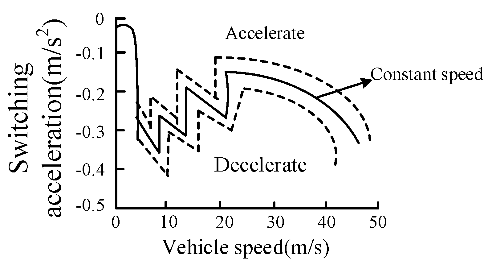
According to the hierarchical control strategy, the lower-level controller converts the desired acceleration command generated by the upper-level controller into corresponding throttle and brake actuator commands. The switching rules between acceleration and deceleration are shown in Figure 3. To improve vehicle driving comfort and reduce the number of accelerations and decelerations, a boundary layer of ±0.03 m/s² is added to the switching curve. In practical intelligent vehicle fleet systems, the lower-level controller mainly consists of throttle and brake actuators.

Considering that the focus of this study is the upper-level finite-time longitudinal cooperative control strategy under disturbances and time-delay, the actuator dynamics are simplified in the lower-level controller. The throttle and brake actuators are assumed to satisfy the desired acceleration commands within their operating ranges. In addition, actuator saturation and gear shifting dynamics are not explicitly modeled, while the engine response lag is indirectly represented by the first-order longitudinal dynamics in Equation (2). Therefore, the lower-level controller mainly serves as an acceleration tracking module for validating the effectiveness of the proposed upper-level controller.

3.2.1. Inverse Engine Model

Assuming that only the longitudinal force is considered and the brake pressure is 0 at vehicle acceleration conditions, the longitudinal vehicle dynamics can be expressed as

$$m_i{a}_{\mathrm{dmd}}=F_t-F_i,$$

(59)

where F_t represents the vehicle driving force.

The driving force is completely provided by the engine. The relationship between the vehicle driving force and the engine torque is

$$F_t={\displaystyle \frac{T_{\mathrm{e}\_\mathrm{dmd}}{i}_g{i}_0{\eta }_t}{r_w}},$$

(60)

where T_{e_dmd} is the engine torque.

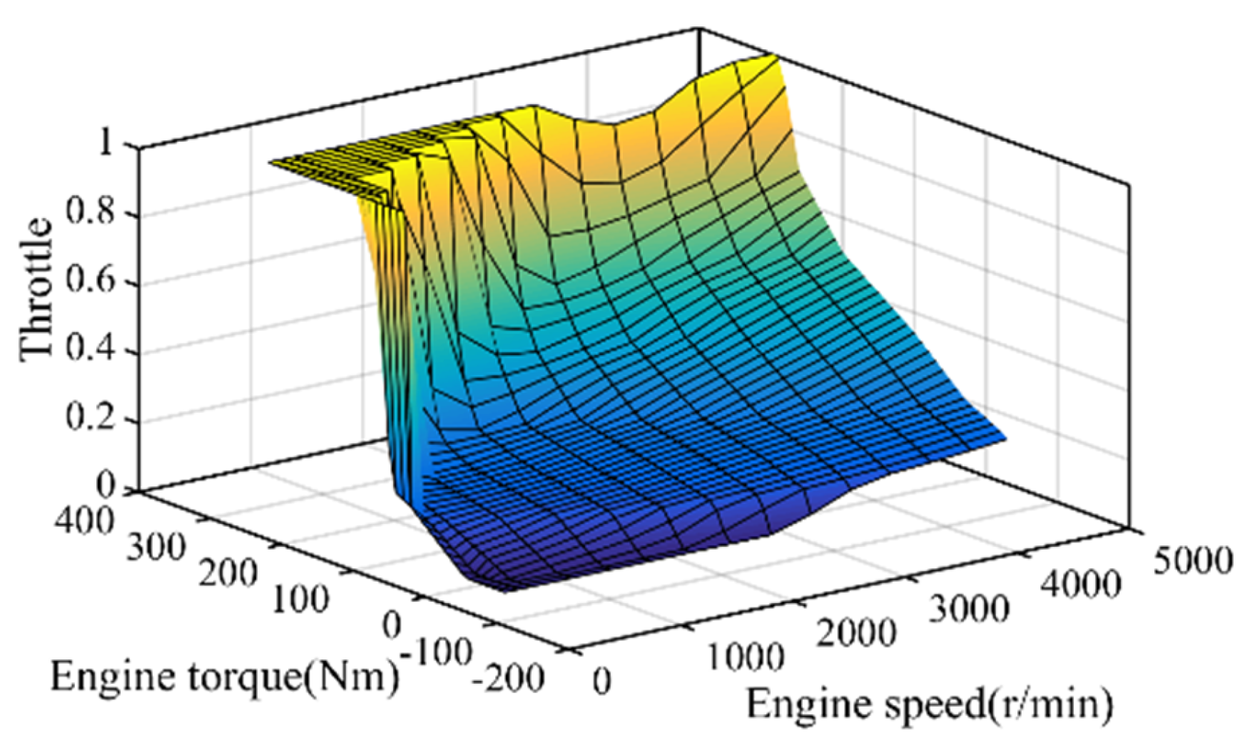
According to the inverse engine torque MAP shown by Figure 4, the throttle opening can be obtained from the engine torque and speed, as calculated by

$${\alpha }_{\mathrm{dmd}}=MAP\left(T_{\mathrm{e}\_\mathrm{dmd}},{\omega }_e\right).$$

(61)

where ω_e is the engine speed. The throttle opening is constrained within the physical operating range of the engine actuator to avoid unrealistic acceleration commands.

3.2.2. Reverse Brake Model

When the vehicle decelerates, it is necessary to control the brake pedal according to the desired deceleration. According to the relationship between the braking force and braking torque, the inverse brake model can be expressed as

$$T_{\mathrm{brk}\_\mathrm{dmd}}={\displaystyle \frac{\left|-m{a}_{\mathrm{dmd}}-F_r\right|}{k_b}}.$$

(62)

where T_{brk_dmd} is the desired braking torque and k_b is the braking system coefficient. The calculated braking torque is limited by the maximum braking capability to ensure feasible deceleration commands under practical operating conditions.

4. Simulation Analysis

To evaluate the effectiveness of the proposed longitudinal finite-time control strategy, an intelligent vehicle fleet consisting of one leading vehicle and four following vehicles is established in the MATLAB/Simulink R2020b environment. The vehicle parameters used in the simulations are listed in

Table 1. Main parameters of vehicle.

Parameter Name	Parameter Value	Unit
Vehicle mass	1370	kg
Vehicle length	4.674	m
Vehicle front area	1.746	m2
Air drag coefficient	0.3	/
Rolling resistance coefficient	0.02	/
Tire radius	0.257	m
Ratio of the main reducer	3.24	/
Ratio of the gearbox	[3.43, 1.81, 1.21, 0.86, 0.6]	/
Mechanical efficiency	0.92	/

. The initial longitudinal positions of the fleet are set as [0 m,−20 m,−40 m,−60 m,−80 m], respectively.

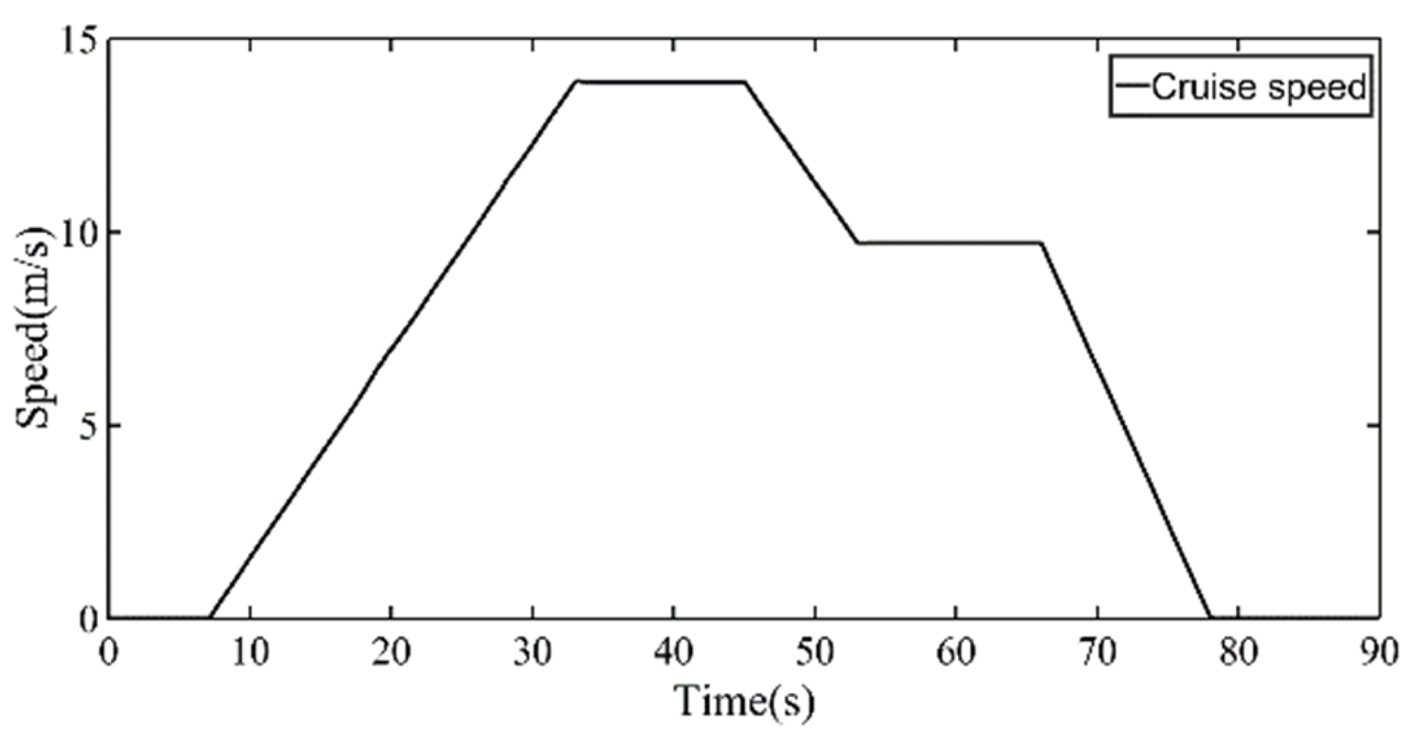
Considering the typical operating characteristics of intelligent vehicle fleet systems in practical urban and highway driving environments, the leading vehicle speed profile includes three representative driving conditions: acceleration, constant-speed cruising, and deceleration, as shown in Figure 5. The vehicle speed is initially 0 m/s. The leading vehicle starts accelerating at t = 7 s and reaches the peak speed of 13.9 m/s, after which the speed remains constant for a period of time. Subsequently, two deceleration maneuvers are introduced to evaluate the transient tracking and disturbance rejection performance of the proposed controller. The total simulation duration is 26 s.

To improve the practical representativeness of the simulation scenarios, both measurement disturbance and communication delay are considered in the intelligent vehicle fleet system. The vehicle speed sensor noise is modeled as bounded random measurement noise acting on the controller input channel. The communication delay is selected within the range of 0.1~0.2 s, which is consistent with the typical delay range reported in intelligent connected vehicle communication systems and vehicle network control studies [28]. The disturbance and delay conditions are simultaneously introduced to evaluate the robustness and finite-time convergence capability of the proposed control strategy under realistic operating conditions.

The simulation model is implemented in MATLAB/Simulink R2020b using a fixed-step solver. The simulation step size is set to 0.001 s to ensure numerical stability and accurate representation of the finite-time control dynamics. The controller parameters, observer gains, PI compensation gains, and NSRL parameters are selected according to the parameter analysis presented in Section 3.1.4.

4.1. Observation Results

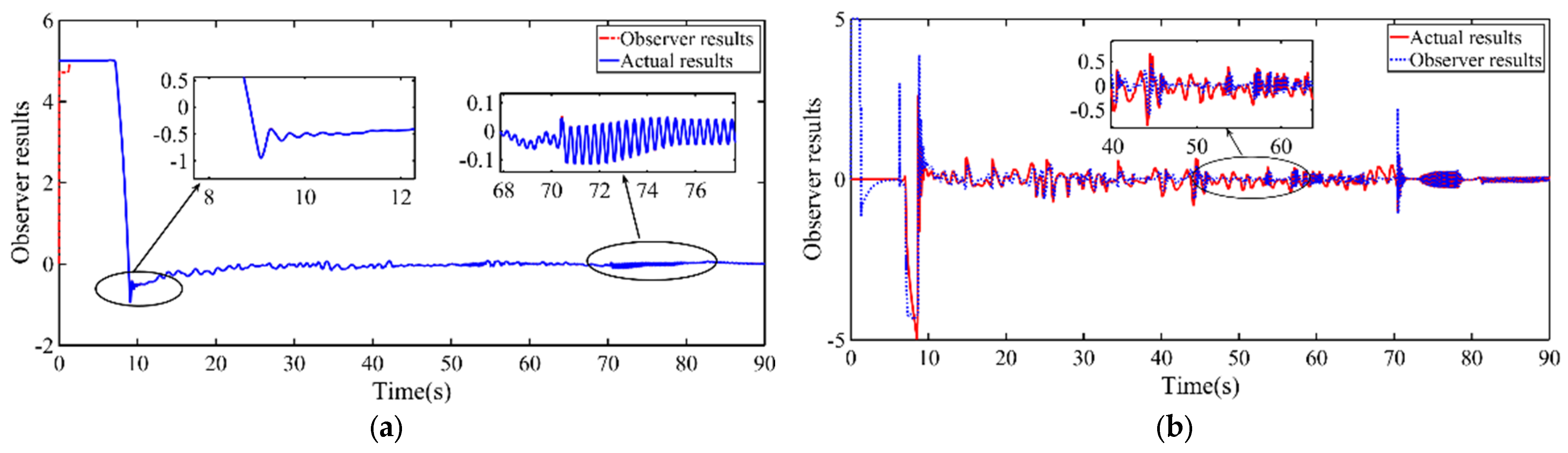
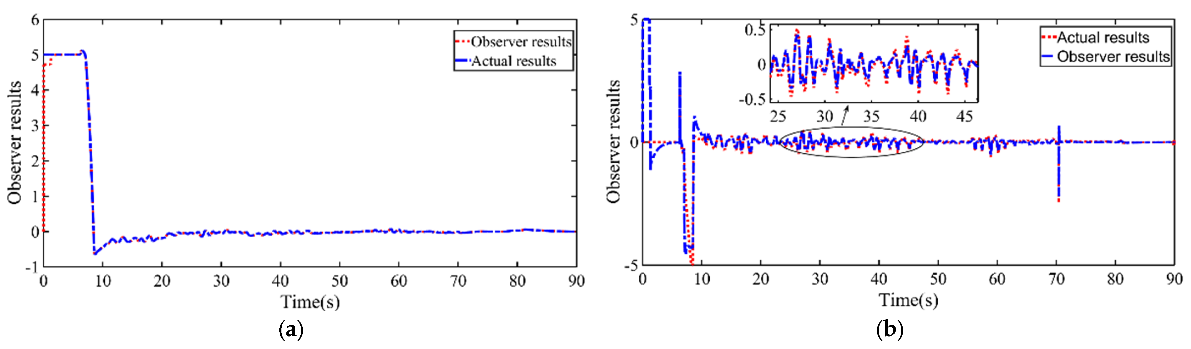
In this study, interference is represented by the measurement noise of the vehicle speed sensor, and random noise is imposed on the third vehicle with a magnitude of ±10%. Figure 6 and Figure 7 compare the observation performance of the FTESO without time-delay compensation and the proposed PFTESO that explicitly considers time-delay effects.

The time-delay in the simulations is selected within the range of [0.1 s, 0.2 s], which is consistent with commonly reported communication and sensing delays in practical vehicle fleet systems. It should be emphasized that this range is not chosen as a critical or limiting stability boundary, but rather as a representative small-delay interval that is sufficient to reveal the influence of time-delay on observer synchronization and control performance.

As can be seen from Figure 6a, the time-delay shows a slight influence on the observation results of z₁, because z₁ only contains the information of the relative vehicle spacing, while the effect of time-delay on the relative spacing is not significant. However, the system time-delay seriously reduces the observation accuracy of z₂, because z₂ contains the information of acceleration and interferences. The time-delay causes the interference information to be out of sync, resulting in a large observation error, as shown by Figure 6b. As illustrated by Figure 7, since the improved Smith predictor can address the issue of time-delay well, the PFTESO based on the Smith predictor achieves accurate observation results for both z₁ and z₂.

To quantitatively evaluate the observation performance, the root mean square error (RMSE) between the observed states and actual states is further calculated, as summarized in

Table 2. Quantitative comparison of observer performance under time-delay conditions.

Observer	z1 RMSE	z2 RMSE	Peak Observation Oscillation
FTESO	0.082	0.214	±0.53
PFTESO	0.021	0.067	±0.18

.

4.2. Simulation Analysis Considering Interference

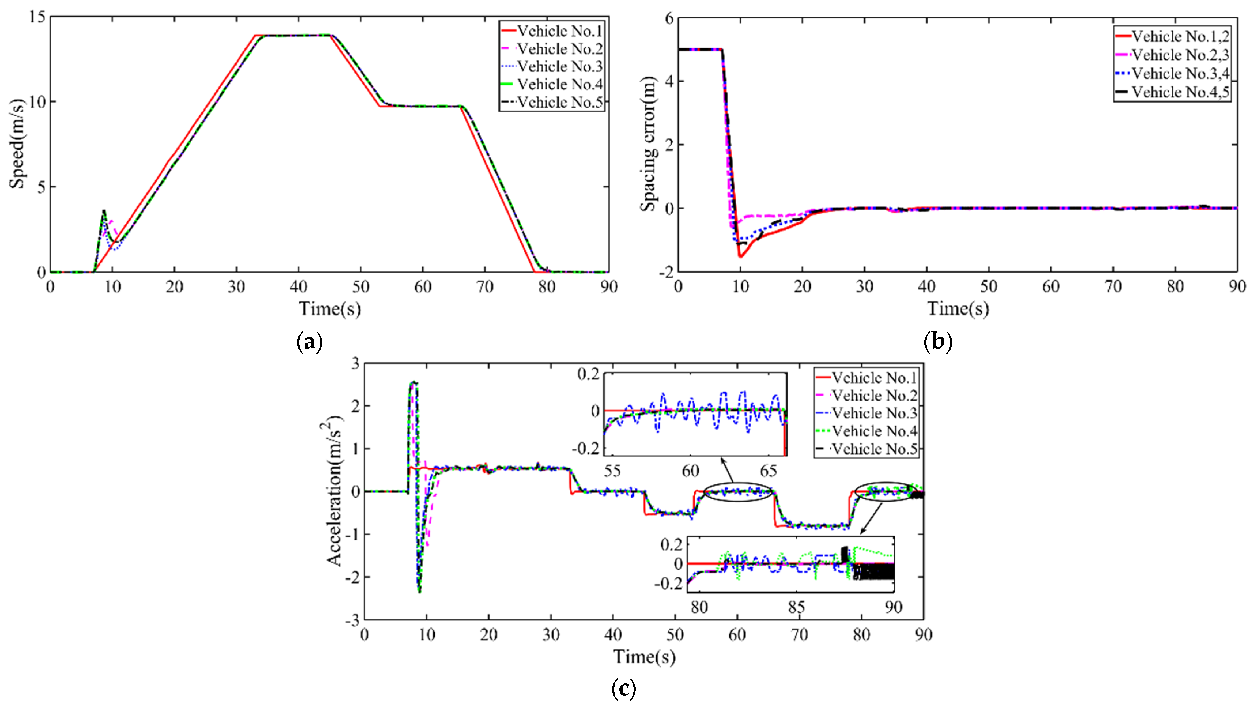
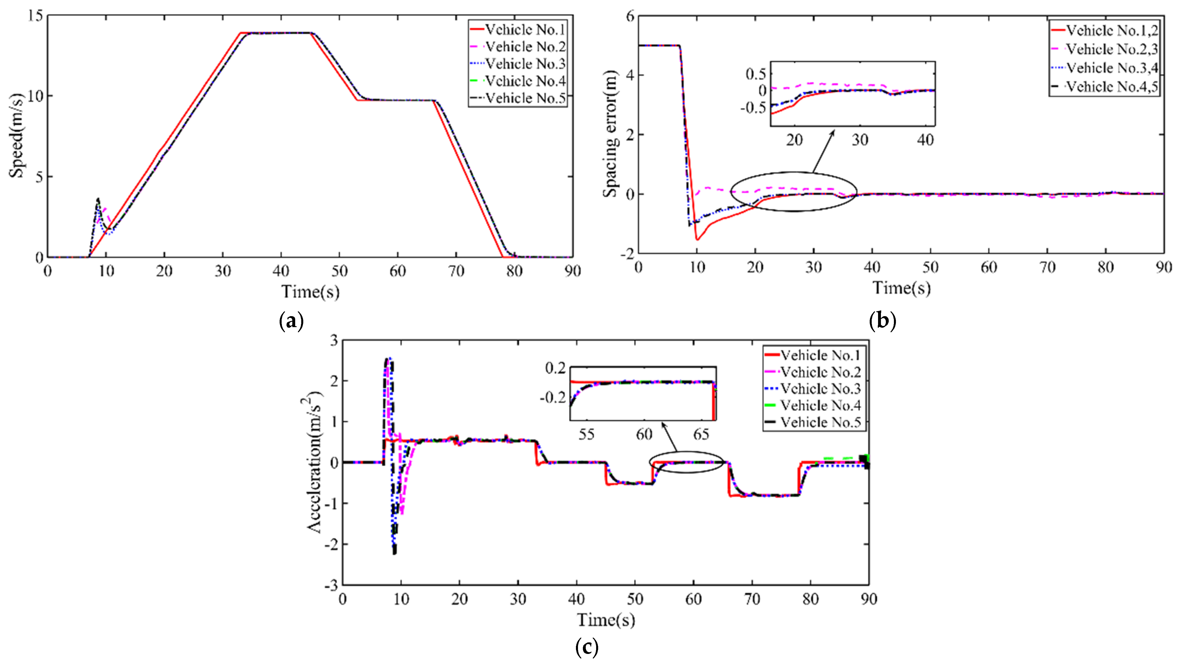
Firstly, the scenario that only considers interference is analyzed. In order to verify the feasibility and superiority of the proposed strategy, the performance of SMC strategy, GFITSMC strategy, and the improved FTESO-GFITSMC strategy are compared. The results with different strategies are compared in Figure 8, Figure 9 and Figure 10.

It can be seen from Figure 8a that when the SMC is used, the maximal overshoot of speed tracking is 3.62%. Due to the influence of speed measurement noise, the velocity of the following vehicles fluctuates slightly when they are stable. As shown by Figure 8b, it takes about 32 s for the vehicle spacing to converge. During the process of the vehicle spacing adjustment, the peak convergence value of vehicle spacing error is around ±1.5 m. Moreover, due to the discontinuity of SMC strategy, there is a chattering phenomenon during the convergence process of the vehicle spacing. Figure 8c shows that, when the first vehicle reaches a constant speed, the acceleration of the following vehicles demonstrate large chattering, which will cause frequent acceleration and deceleration of the following vehicles and affect driving comfort.

Different from the SMC strategy, the GFITSMC eliminates the speed fluctuation phenomenon, and the speed of the following vehicles is still relatively stable even with measurement noise, as shown by Figure 9a. It can be observed from Figure 9b that the relative distance between vehicles can converge rapidly, and the final convergence time is 13 s. In addition, when the speed changes again from constant speed, the vehicle spacing error does not change significantly. As can be seen from Figure 9c, since the GFITSMC neglects the influence of noise, local chattering occurs in the acceleration of the following vehicles, and the chattering amplitude is about ±0.08 m/s². However, the variation amplitude of the switching boundary layer for the acceleration and deceleration is only 0.03 m/s². Consequently, the chattering of this amplitude will still result in frequent acceleration and deceleration of the vehicle.

Compared with the GFITSMC, as shown by Figure 9a,b and Figure 10a,b, the proposed FTESO-GFITSMC demonstrates similar performance to the GFITSMC in terms of vehicle speed tracking and spacing control. The dynamic convergence performance of the system with the proposed FTESO-GFITSMC is not affected. On the other hand, since the speed noise interference is observed in advance using the FTESO and the influence of noise is considered in the controller design process, the FTESO-GFITSMC strategy significantly suppresses the vehicle acceleration chattering phenomenon, as shown by Figure 10c.

Based on the above analysis, the performance comparison of the longitudinal control strategy for an intelligent vehicle fleet considering mismatching disturbances can be further obtained, as shown in

Table 3. Performance comparison of longitudinal control strategies for intelligent vehicle fleet under mismatched disturbances.

Performance Index	SMC	GFITSMC	FTESO-GFITSMC
Maximum vehicle speed overshoot	3.62%	0.43%	0.36%
Relative inter-vehicle spacing convergence time	32 s	13 s	28 s
Steady-state relative inter-vehicle spacing error	0.06 m	0.06 m	0.04 m
Peak inter-vehicle spacing error	±1.5 m	−1.7 m	−1.7 m
Peak acceleration chattering	±0.23 m/s2	±0.08 m/s2	0.03 m/s2

.

4.3. Simulation Analysis Considering Both Interference and Time-Delay

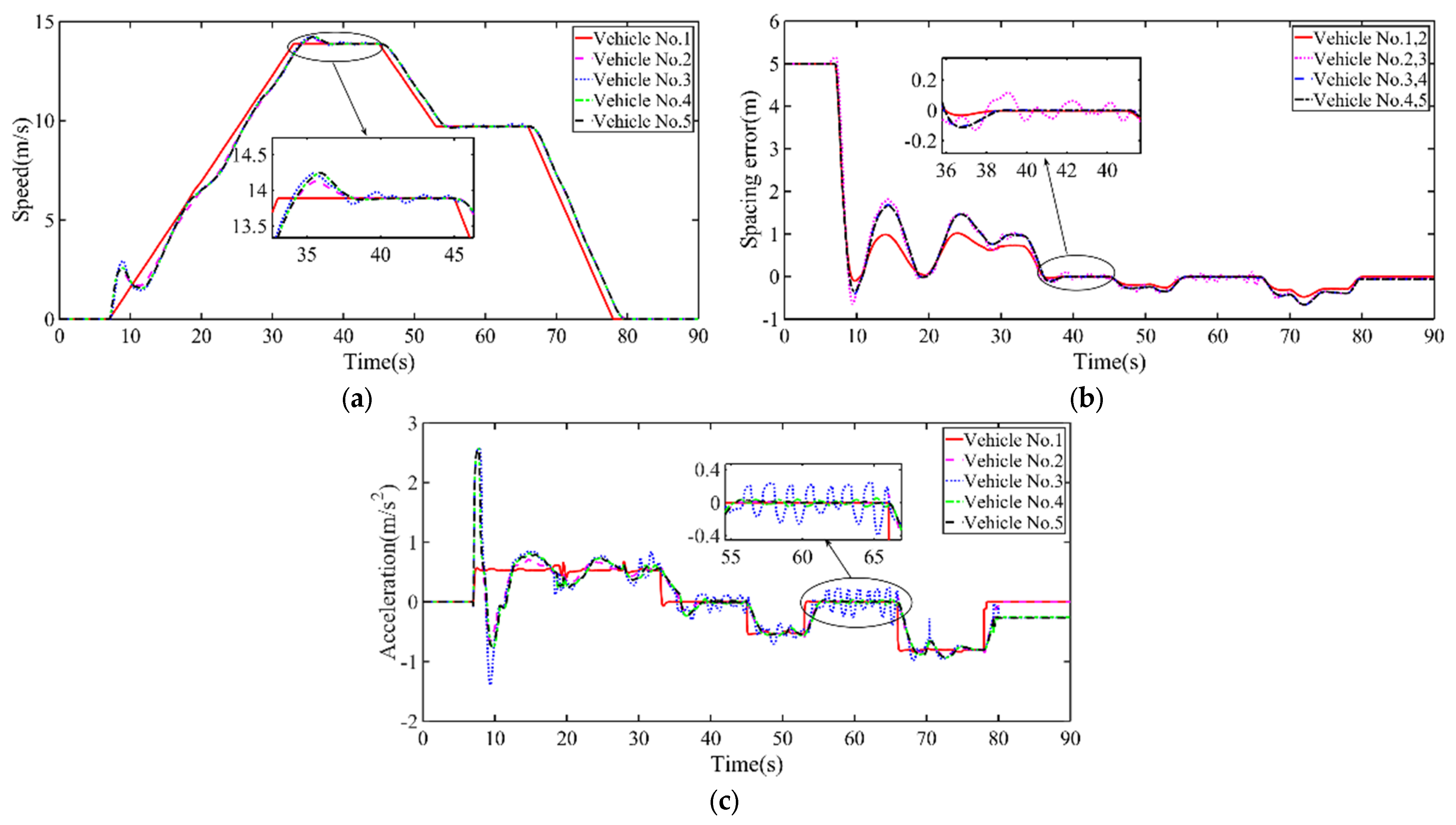
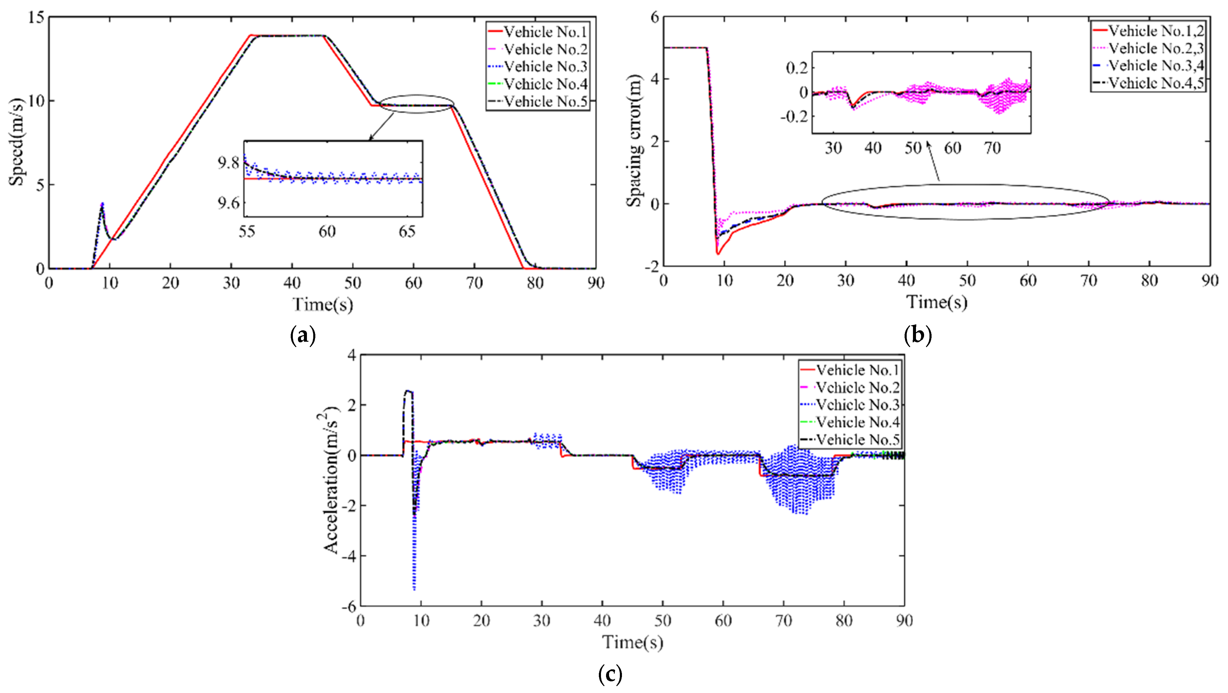
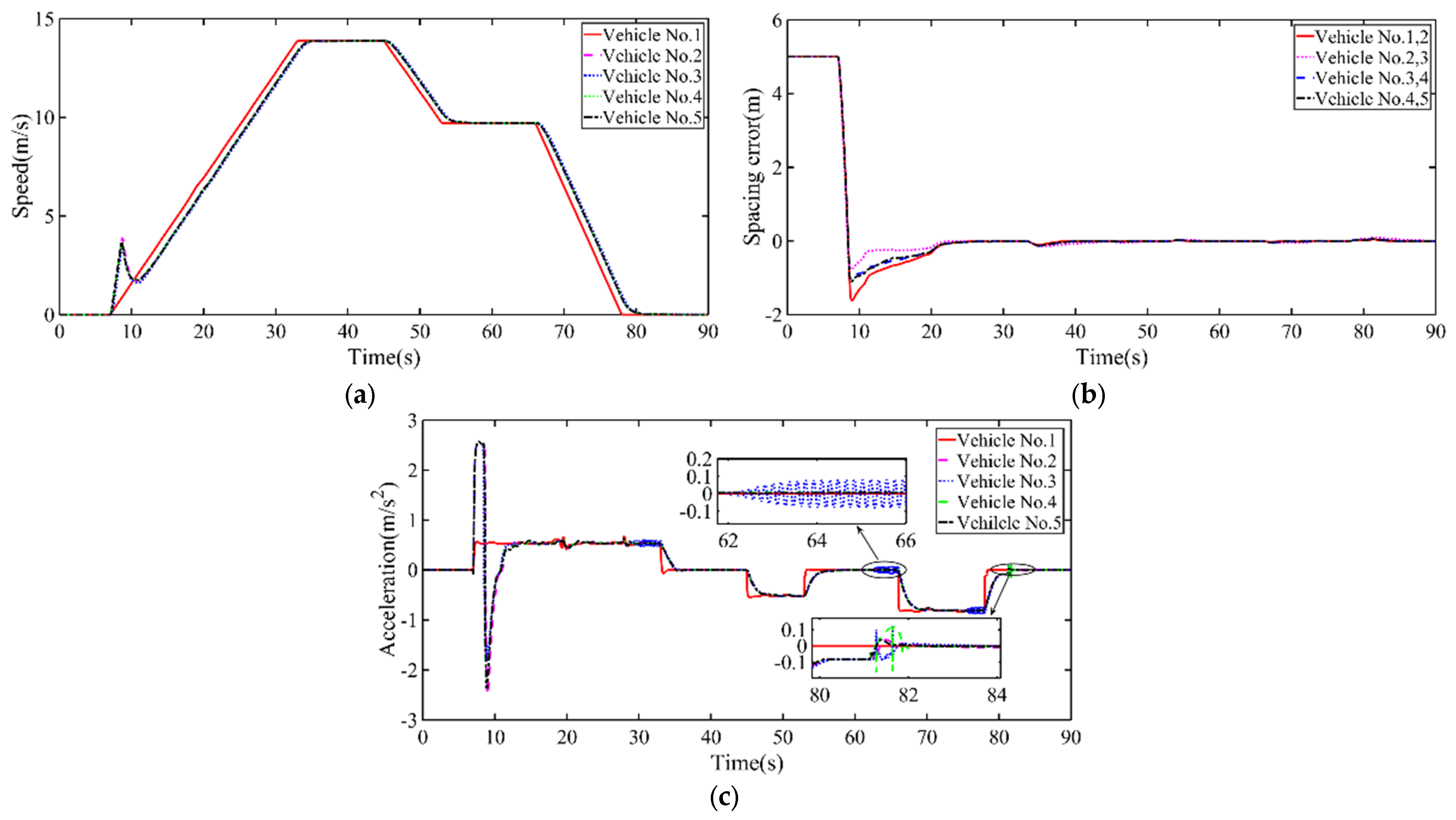
Using the communication time-delay between the third vehicle and other vehicles as an example, and randomly setting the time-delay in the time intervals of [0.1 s, 0.2 s], Figure 11, Figure 12 and Figure 13 respectively show the comparison results of the delay-free prediction strategy, the Smith time-delay prediction strategy, and our proposed improved Smith time-delay prediction strategy.

When the time-delay prediction is not adopted and the leading vehicle in the fleet is driving at a constant speed, the speed of the following vehicles in the fleet will fluctuate frequently, as shown by Figure 11a. At the same time, due to the time-delay of information interaction, the current following vehicle fails to obtain the state information of other vehicles in time, then the FTESO cannot accurately predict the interference value, resulting in an obvious and frequent chattering of relative distance between vehicles, which reduces the steady-state accuracy of vehicle spacing convergence, as shown by Figure 11b. This is detrimental to the safety and efficiency of the fleet. In fact, due to the time-delay between vehicles, the acceleration amplitude of the third vehicle increases significantly. When the speed of the leading vehicle changes again from a stable state, the acceleration of the third vehicle will also change with high frequency, which will cause the following vehicles to accelerate and decelerate frequently, as shown by Figure 11c, which will deteriorate driving comfort and even affect normal driving of the vehicle.

Compared with the delay-free prediction strategy, the Smith time-delay prediction strategy can ensure stable tracking of vehicle speed. Since the delay coefficient is predicted in advance, the time-delay of information communication does not affect the stability of vehicle speed tracking, as shown by Figure 12a, which indicates that Smith time-delay prediction is effective in alleviating the negative impact of time-delay. As shown by Figure 12b, the convergence process of vehicle relative spacing also becomes obviously stable, eliminating the fluctuation phenomenon of vehicle spacing error. However, due to the time-delay prediction error of the Smith predictor, the acceleration of the following vehicle still fluctuates at steady states. In particular, in the time interval of 60 s~80 s, when the vehicle decelerates from a constant speed, the acceleration chattering amplitude exceeds the acceleration and deceleration switching layer, leading to frequent acceleration switching. Compared with the delay-free prediction strategy, significant improvement in driving comfort is not observed, as shown by Figure 12c.

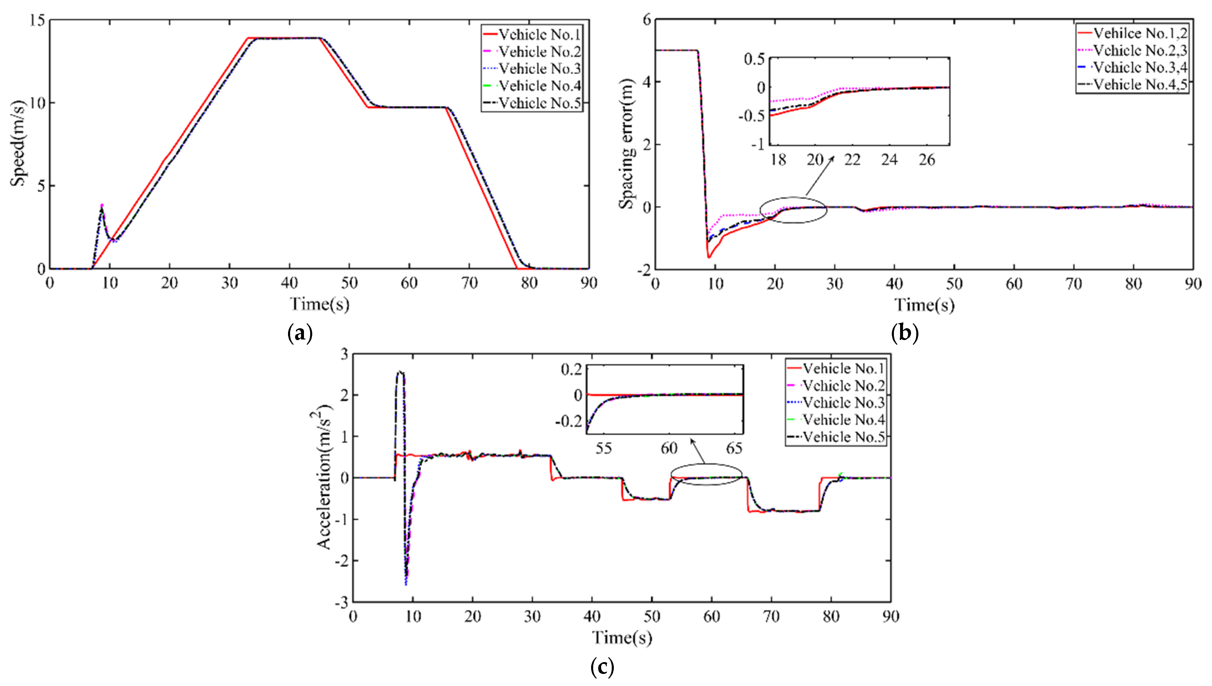
Compared with the previous two strategies, the improved Smith time-delay prediction strategy proposed in this paper ensures stable tracking of vehicle speed, as shown by Figure 13a, and stable driving of the fleet. Meanwhile, the finite-time convergence of vehicle relative spacing is realized, as shown by Figure 13b. The convergence time is about 13 s. Simulation results validate the feasibility and effectiveness of the strategy. Due to the application of a PI controller as the compensation control of the ideal acceleration, control accuracy is improved. Although the acceleration amplitude increases at the initial moment, the acceleration is still within a reasonable range and is acceptable, as shown by Figure 13c.

Based on the above analysis, the performance comparison of the longitudinal control strategies for an intelligent vehicle fleet considering interference and time-delay can be further obtained, as shown in

Table 4. Performance comparison of intelligent fleet longitudinal control strategies considering both interference and time-delay.

Performance Index	Delay-Free Prediction	Smith Prediction	FTESO-GFITSMC
Maximum vehicle speed overshoot	1.12%	0.23%	0.29%
Relative inter-vehicle spacing convergence time	32 s	13 s	13 s
Steady-state relative inter-vehicle spacing error	0.02 m	0.01 m	0.01 m
Peak inter-vehicle spacing error	±1.7 m	−1.7 m	−1.7 m
Peak acceleration chattering	±5.61 m/s2	±0.1 m/s2	0 m/s2

.

5. Conclusions

This study addresses the slow convergence problem of an intelligent vehicle fleet under the combined influence of mismatched disturbances and system time-delay. Considering the influence of vehicle speed measurement noise, a finite-time extended state observer (FTESO) is designed to estimate disturbance information. To alleviate the asynchronous observer input problem caused by time-delay, an improved Smith predictor is incorporated into the FTESO to construct a predictive finite-time extended state observer (PFTESO). On this basis, a global fast integral terminal sliding mode controller (GFITSMC) combined with proportional–integral (PI) compensation is developed to improve the robustness and finite-time convergence performance of the intelligent vehicle fleet system.

Comparative simulations under disturbance-only conditions and combined disturbance-delay conditions are conducted to evaluate the effectiveness of the proposed strategy. The simulation results demonstrate that the proposed PFTESO significantly improves disturbance observation accuracy under delayed conditions, where the RMSE values of z₁ and z₂ are reduced from 0.082 and 0.214 to 0.021 and 0.067, respectively. In addition, compared with conventional control strategies, the proposed FTESO-GFITSMC effectively suppresses acceleration chattering from ±0.23 m/s² to 0.03 m/s² while maintaining satisfactory finite-time convergence performance. Under the combined influence of disturbances and time-delay, the proposed strategy achieves a convergence time of 13 s and demonstrates improved robustness and control accuracy for the intelligent vehicle fleet.