Sustainable Multi-Energy Microgrid Operation: Birds of Prey-Based Day-Ahead Scheduling Under Seasonal Renewable Uncertainty

Abstract

The increasing integration of renewable energy resources into modern microgrids requires reliable scheduling methods capable of managing uncertainty, seasonal variability, operating cost, and environmental impact. This study proposes a stochastic day-ahead scheduling approach for a representative grid-connected multi-energy microgrid comprising photovoltaic generation, wind generation, a microturbine, a fuel cell, an energy storage system, and utility-grid exchange. The proposed model was implemented and simulated in a MATLAB (2024b) environment. The Birds of Prey-Based Optimization algorithm is applied to determine the optimal 24 h dispatch schedule by minimizing a weighted objective function that combines operating and emission costs. Uncertainties in solar irradiance, wind speed, electrical load, ambient temperature, and electricity prices are modeled using probabilistic distributions and Monte Carlo simulations. To improve computational efficiency, 1000 generated scenarios are reduced to 10 representative scenarios using Fast Forward Selection based on Kantorovich distance. Seasonal case studies for winter, spring, summer, and autumn are used to evaluate the proposed method. Compared with five metaheuristic algorithms, the proposed approach achieves the lowest fitness value in all seasons, with reductions of 15.2%, 26.5%, 6.8%, and 23.9%, respectively. The results confirm improved economic and environmental microgrid operation under seasonal renewable uncertainty.

1. Introduction

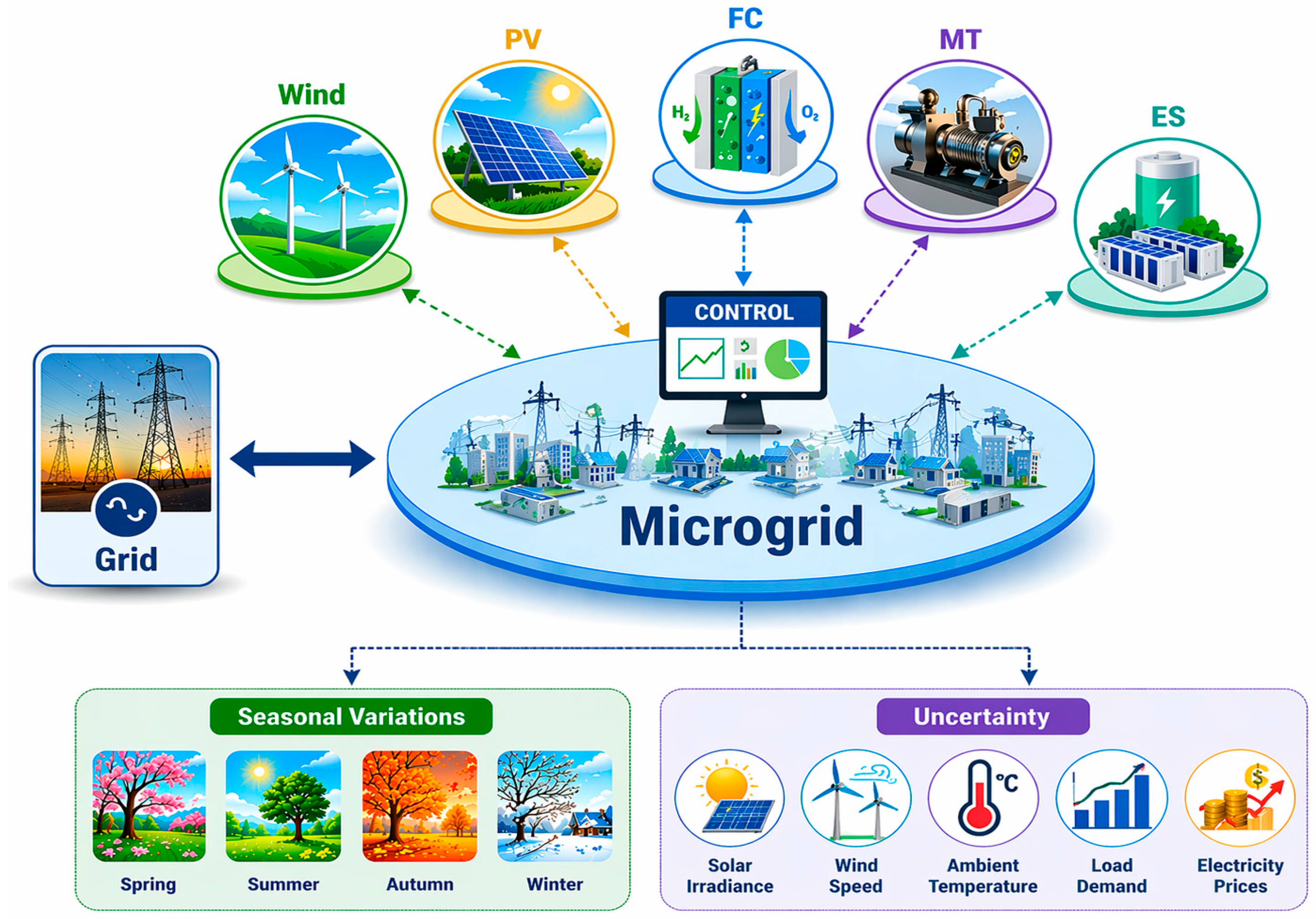
The incorporation of renewable energy technologies has become increasingly prominent in the global energy transition, owing to their capacity to mitigate carbon emissions and promote long-term energy sustainability [1,2]. Distributed generation (DG) resources, such as wind turbines (WTs), photovoltaic (PV) systems, microturbines (MTs), fuel cells (FCs), and energy storage (ES) systems, are expected to play a central role in the future energy landscape. To effectively harness the potential of these non-conventional resources, grid integration is essential [3]. Consequently, microgrids (MGs), especially those incorporating renewable resources, have emerged as key enablers for improving the efficiency and sustainability of modern power systems while reducing environmental pollution [4]. An MG represents the coordinated management and control of multiple DG units in conjunction with various ES systems [5]. Beyond simply meeting local load requirements by drawing energy from both the grid and conventional power sources, the MG also enhances grid resilience, mitigates system disturbances, and serves as a valuable grid-supporting asset that enables faster system response and recovery [6].

Day-ahead scheduling is therefore essential for achieving reliable and economical operation of grid-connected MGs. In a multi-energy MG, the energy management system must coordinate renewable generation, dispatchable units, storage charging/discharging, and utility-grid exchange while satisfying technical and economic constraints. Recent studies confirm that MG scheduling under renewable uncertainty remains an active research area because the dispatch problem is nonlinear, constrained, and strongly affected by stochastic input variables. For example, recent work on hybrid solar–wind MGs has shown that advanced energy-management strategies can improve the coordination of renewable generation, storage systems, FCs, and grid interaction under variable operating conditions [7]. A recent stochastic mixed-integer linear programming (MILP) framework has also been proposed for renewable-rich MG dispatch, emphasizing the importance of uncertainty-aware scheduling when renewable penetration is high [8].

Several optimization approaches have been developed for MG energy management. Mathematical programming methods, such as mixed-integer linear programming, provide structured dispatch solutions and are useful when the problem can be formulated in a tractable linear or mixed-integer form [8]. Nevertheless, MG scheduling often includes nonlinear component models, storage dynamics, nonconvex operational constraints, and coupled hourly decisions. For this reason, metaheuristic optimization methods have been widely used to solve complex MG scheduling problems. Recent studies have applied a modified multi-objective manta-ray foraging optimization for hybrid MGs [7], modified marine predators optimization for renewable MGs with ES and electricity price effects [9], Particle swarm optimization for hybrid renewable MG operation with reserve-margin consideration [10], improved differential evolution (DE) for multi-MG scheduling [11], Golden Jackal Optimization for hybrid-source MG energy management [12], and Honey Badger Algorithm-based scheduling for MG cost and emission reduction [13].

In addition to classical and nature-inspired optimization techniques, learning-based and forecasting-assisted approaches have recently been introduced to improve energy-management performance. Deep Reinforcement Learning (DRL) has been used for day-ahead and intra-day scheduling of multi-source energy storage systems, showing the potential of learning-based control under variable renewable conditions [14]. Probabilistic forecasting combined with robust multi-objective optimization has also been applied to renewable MG scheduling to improve decision-making under uncertain renewable output and load behavior [15]. These studies demonstrate a growing interest in combining optimization, forecasting, and uncertainty modeling. However, learning-based methods may require large training datasets and careful tuning, while robust and mathematical programming approaches may become computationally demanding when the scheduling model includes nonlinear multi-energy components and large uncertainty sets.

Uncertainty modeling is another essential aspect of renewable-rich MG scheduling. Monte Carlo (MC) simulation is commonly used to represent stochastic variations in solar irradiance, wind speed, electrical load, ambient temperature, and electricity prices. By generating many possible scenarios, MC simulation can capture the probabilistic behavior of uncertain variables over the scheduling horizon. However, directly using a large scenario set in the optimization problem increases the computational burden. Scenario-reduction methods, such as Fast Forward Selection (FFS), can reduce this complexity by selecting a smaller number of representative scenarios while preserving the main statistical features of the original scenario population. Recent stochastic dispatch studies have used fast-forward scenario reduction to reduce the size of uncertainty scenarios in renewable-rich energy systems, confirming the usefulness of this approach for computationally efficient stochastic scheduling [16].

While stochastic modeling techniques improve the representation of renewable and load uncertainties, many existing studies still overlook the seasonal variability of renewable resources and demand patterns. In [7], an energy management scheme for a hybrid solar–wind MG was developed by employing a modified multi-objective manta ray foraging optimizer (MOMRFO). Their method coordinated power allocation, load shifting, and storage operation to drive down operating costs, reduce emissions, and improve user satisfaction. Simulation results showed that the proposed framework delivered markedly better performance and achieved greater cost reductions than both conventional and recently introduced optimization approaches. In [17], a hybrid quadratic interpolation and new local search graylag goose optimization approach was proposed for energy management in multi-energy MGs. The method improved renewable uncertainty handling through enhanced forecasting, off-design device modeling, and multi-timescale scheduling, achieving superior operational performance. However, the approach strongly relies on forecasting accuracy and lacks robust adaptive uncertainty management. In addition, its high algorithmic complexity may limit practical real-time implementation. The authors of [9] studied the impact of V2G-enabled electric vehicles on MG operation under uncertainty using the unscented transformation and a modified marine predators algorithm. The approach improved dispatch coordination, lowered power losses, and reduced operating costs. However, the work focused mainly on economic objectives, with limited attention to emission reduction or adaptive intelligent control strategies for highly dynamic operating conditions. A multi-timescale scheduling framework was proposed in [14] to address renewable energy variability in day-ahead and intra-day operations. By combining a day-ahead optimization layer with an attention-guided DRL Actor–Critic model, the method adapted effectively to real-time deviations. Case studies on the East China grid have demonstrated improved renewable absorption, system flexibility, and operational economy. In a related contribution [8], a multi-objective MILP framework was developed for MG scheduling with renewable sources, ES, and demand response. The model improved economic, environmental, and technical performance in both operating modes while benefiting from real-time pricing and load flexibility. However, the approach remains largely deterministic and computationally intensive, limiting its effectiveness under stochastic and seasonal operating conditions. Summaries of some reported methods employed for managing the energy of MGs are discussed in Table 1.

Although the above studies provide important contributions, several research gaps remain. First, many MG scheduling studies evaluate system operation under a single representative day or limited operating condition, which may not fully capture seasonal variations in renewable generation, demand, storage behavior, grid exchange, operating cost, or emission costs. Second, some studies consider uncertainty modeling but do not provide sufficient integration between MC scenario generation, scenario reduction, and seasonal dispatch analysis. Third, many metaheuristic comparisons report numerical superiority without explaining how seasonal operating conditions affect the difficulty of the scheduling problem and the behavior of different algorithms. Finally, the Birds of Prey-Based Optimization (BPBO) algorithm, recently introduced as a metaheuristic inspired by the hunting strategies of predatory birds, has not yet been sufficiently explored for stochastic day-ahead multi-energy MG scheduling under seasonal renewable uncertainty [18]. BPBO is particularly attractive because its individual hunting, cooperative hunting, competitive movement, and continued-search mechanisms provide a balance between exploration and exploitation.

To address these gaps, this study proposes a stochastic day-ahead scheduling framework for a grid-connected multi-energy MG under seasonal renewable uncertainty. The MG surveys include PV generation, wind generation, MT, FC, ESS, and utility-grid exchange. The uncertain variables include solar irradiance, wind speed, ambient temperature, electrical load demand, and electricity price. MC simulation is used to generate stochastic operating scenarios, and FFS based on Kantorovich distance is applied to reduce the original scenario set from 1000 scenarios to 10 representative scenarios. The reduced scenario set is then used in the BPBO-based scheduling model to minimize a weighted objective function including operating cost and emission cost.

The main contributions of this work are summarized as follows:

• A stochastic day-ahead scheduling model is developed for a grid-connected multi-energy MG including PV, WT, MT, FC, ESS, and utility-grid exchange.
• Solar irradiance, wind speed, electrical load, ambient temperature, and electricity price uncertainties are modeled probabilistically, and an MC simulation is used to generate uncertainty scenarios.
• FFS, based on Kantorovich distance, is applied to reduce 1000 MC scenarios to 10 representative scenarios, improving computational efficiency while preserving the dominant statistical characteristics of the uncertainty set.
• The BPBO algorithm is adapted to solve the constrained MG scheduling problem and to coordinate dispatchable generation, renewable generation, storage operation, and grid transactions.
• Seasonal case studies are conducted for winter, spring, summer, and autumn to evaluate the economic and environmental effects of renewable uncertainty, load variation, and seasonal operating conditions.
• The performance of BPBO is compared with several metaheuristic algorithms using best, mean, worst, standard deviation, convergence behavior, computational time, and seasonal cost–emission analysis.

The remainder of this paper is organized as follows. Section 2 presents the MG system model and component equations. Section 3 describes the uncertainty modeling, MC scenario generation, and scenario-reduction procedure. Section 4 formulates the objective function and operational constraints. Section 5 explains the BPBO algorithm and its application to the scheduling problem. Section 6 presents and discusses the simulation results. Section 7 concludes the paper and outlines future research directions.

Table 1. Summary of some reported methods employed for managing the energy of MGs.

Ref.	Reference (Year)	Resources					Uncertainty	Seasonal Variation	Optimizer	Objective Function
		PV	Wind	ES	FC	MT				Cost	Emissions
[7]	2025	√	√	√	√	×	×	×	MOMRFO	√	√
[17]	2025	√	√	√	×	×	√	△	Modified Graylag Goose Optimization	√	×
[9]	2025	√	√	√	√	√	√	×	Modified Marine Predators Algorithm	√	×
[14]	2025	×	√	√	×	×	√	×	Attention-Based DRL	√	×
[8]	2025	√	√	√	×	×	√	×	Multi-Stage Stochastic MILP	√	×
[10]	2024	√	√	√	×	×	√	×	PSO	√	×
[11]	2024	√	√	√	×	×	√	△	Improved Differential Evolution Algorithm	√	√
[19]	2024	√	√	√	×	×	×	×	Improved Ant Lion Optimizer	√	×
[12]	2024	√	√	√	√	√	×	×	Golden Jackal Optimization	√	×
This study	This study	√	√	√	√	√	√	√	The Proposed PBPO	√	√
Ref.	Main Limitation/Gap Relative to this Work
[7]	Does not include MT, probabilistic uncertainty modeling, seasonal analysis, or MC–FFS scenario reduction.
[17]	Considers RES uncertainty, but lacks FC/MT, FFS-based scenario reduction, and detailed seasonal cost–emission dispatch.
[9]	Focuses mainly on operating-cost minimization; emission objective and seasonal MC–FFS analysis are not included.
[14]	Mainly focuses on multi-source storage and wind-power scheduling, not full PV–WT–ES–FC–MT microgrid dispatch.
[8]	Handles renewable uncertainty, but does not include FC/MT, emission objective, BPBO, or four-season scenario-reduced scheduling.
[10]	Considers PV–WT–BESS operation under uncertainty, but lacks FC/MT, emission objective, and seasonal stochastic scenario reduction.
[11]	Includes uncertainty and environmental cost terms, but lacks FC/MT, BPBO, MC–FFS reduction, and full four-season analysis.
[19]	Wind–solar–storage cost-focused study; does not include FC/MT, stochastic uncertainty, seasonal analysis, or emissions.
[12]	Includes a broad MG resource set but is mainly deterministic and cost-focused; uncertainty, seasonal analysis, and emission optimization are not central.
This study	Addresses the gap by combining PV, WT, ES, FC, MT, stochastic uncertainty, MC–FFS/Kantorovich scenario reduction, seasonal analysis, and cost–emission optimization.

Note: √ = considered; × = not considered; △ = partially/indirectly considered, but not as a full four-season stochastic analysis.

Table 1. Summary of some reported methods employed for managing the energy of MGs.

Ref.	Reference (Year)	Resources					Uncertainty	Seasonal Variation	Optimizer	Objective Function
		PV	Wind	ES	FC	MT				Cost	Emissions
[7]	2025	√	√	√	√	×	×	×	MOMRFO	√	√
[17]	2025	√	√	√	×	×	√	△	Modified Graylag Goose Optimization	√	×
[9]	2025	√	√	√	√	√	√	×	Modified Marine Predators Algorithm	√	×
[14]	2025	×	√	√	×	×	√	×	Attention-Based DRL	√	×
[8]	2025	√	√	√	×	×	√	×	Multi-Stage Stochastic MILP	√	×
[10]	2024	√	√	√	×	×	√	×	PSO	√	×
[11]	2024	√	√	√	×	×	√	△	Improved Differential Evolution Algorithm	√	√
[19]	2024	√	√	√	×	×	×	×	Improved Ant Lion Optimizer	√	×
[12]	2024	√	√	√	√	√	×	×	Golden Jackal Optimization	√	×
This study	This study	√	√	√	√	√	√	√	The Proposed PBPO	√	√
Ref.	Main Limitation/Gap Relative to this Work
[7]	Does not include MT, probabilistic uncertainty modeling, seasonal analysis, or MC–FFS scenario reduction.
[17]	Considers RES uncertainty, but lacks FC/MT, FFS-based scenario reduction, and detailed seasonal cost–emission dispatch.
[9]	Focuses mainly on operating-cost minimization; emission objective and seasonal MC–FFS analysis are not included.
[14]	Mainly focuses on multi-source storage and wind-power scheduling, not full PV–WT–ES–FC–MT microgrid dispatch.
[8]	Handles renewable uncertainty, but does not include FC/MT, emission objective, BPBO, or four-season scenario-reduced scheduling.
[10]	Considers PV–WT–BESS operation under uncertainty, but lacks FC/MT, emission objective, and seasonal stochastic scenario reduction.
[11]	Includes uncertainty and environmental cost terms, but lacks FC/MT, BPBO, MC–FFS reduction, and full four-season analysis.
[19]	Wind–solar–storage cost-focused study; does not include FC/MT, stochastic uncertainty, seasonal analysis, or emissions.
[12]	Includes a broad MG resource set but is mainly deterministic and cost-focused; uncertainty, seasonal analysis, and emission optimization are not central.
This study	Addresses the gap by combining PV, WT, ES, FC, MT, stochastic uncertainty, MC–FFS/Kantorovich scenario reduction, seasonal analysis, and cost–emission optimization.

Note: √ = considered; × = not considered; △ = partially/indirectly considered, but not as a full four-season stochastic analysis.

2. System Modeling and Components

The MG architecture investigated in this study comprises multiple distributed energy resources operating in coordination to meet local electrical demand while minimizing operational costs and environmental emissions. The system integrates both dispatchable and non-dispatchable generation units alongside ES capabilities and maintains connectivity to the grid for bidirectional power exchange, as displayed in Figure 1.

2.1. Microturbine Unit

The MT is considered a dispatchable generation unit in the studied MG. It supplies controllable electrical power when the available renewable generation and ES output are insufficient to meet the load demand. The MT is therefore important for maintaining the power balance, especially during periods of low PV and WT generation or high electricity demand. Since the MT consumes fuel during operation, its generation cost is represented using a quadratic fuel-cost function. The operational cost associated with MT generation at any time interval is expressed through a quadratic fuel cost function [20]:

$$C_{\mathrm{MT}}\left(t\right)=a_{\mathrm{MT}}{P}_{\mathrm{MT}}^2\left(t\right)+b_{\mathrm{MT}}{P}_{\mathrm{MT}}\left(t\right)+c_{\mathrm{MT}}$$

(1)

where $P_{\mathrm{MT}}\left(t\right)$ represents the MT power output at time $t$ (kW), $a_{\mathrm{MT}}$ denotes the quadratic fuel cost coefficient ($/kW²), $b_{\mathrm{MT}}$ signifies the linear fuel cost coefficient ($/kW), and $c_{\mathrm{MT}}$ indicates the fixed operational cost ($).

2.2. Fuel Cell System

The FC is also modeled as a dispatchable power source in the MG. Compared with conventional fuel-based generation units, the FC can provide electrical power with relatively lower emissions and stable operating performance. In the proposed scheduling model, the FC contributes to meeting the demand when renewable generation and ES are not sufficient. Its operating cost is also represented by a quadratic cost function. The operating cost of the FC at hour $t$ is given by [20]:

$$C_{\mathrm{FC}}\left(t\right)=a_{\mathrm{FC}}{P}_{\mathrm{FC}}^2\left(t\right)+b_{\mathrm{FC}}{P}_{\mathrm{FC}}\left(t\right)+c_{\mathrm{FC}}$$

(2)

where $P_{\mathrm{FC}}\left(t\right)$ represents FC power output (kW), while $a_{\mathrm{FC}}$, $b_{\mathrm{FC}}$, and $c_{\mathrm{FC}}$ are the corresponding cost coefficients with units analogous to the MT parameters.

2.3. Photovoltaic Generation

PV panels convert solar irradiance into electrical power, with output dependent on environmental conditions. The instantaneous PV power generation is modeled as [21,22]:

$$P_{PV}^{available}\left(t\right)=A_{\mathrm{PV}}·{\eta }_r·{\eta }_t·G\left(t\right)·[1-\beta (T_c\left(t\right)-T_r\left)\right]$$

(3)

where $A_{\mathrm{PV}}$ denotes the total panel area (m²), ${\eta }_r$ represents reference conversion efficiency, ${\eta }_t$ indicates maximum power point tracking efficiency, G(t) is solar irradiance (kW/m²), β specifies the temperature coefficient (°C⁻¹), $T_c\left(t\right)$ represents cell temperature (°C), and $T_r$ denotes reference temperature (°C). The cell temperature relates to ambient conditions through:

$$T_c(t)=T_a(t)+{\displaystyle \frac{\mathrm{NOCT}-20}{0.8}}·G(t)$$

(4)

where $T_a\left(t\right)$ is the ambient temperature (°C), and NOCT represents the nominal operating cell temperature (°C).

2.4. Wind Turbine System

Wind power generation exhibits nonlinear dependence on wind speed, described by a piecewise function reflecting cut-in, rated, and cut-out speed characteristics [23]:

$$P_{\mathrm{wind}}^{\mathrm{available}}\left(t\right)=\left\{\begin{array}{cc}0,& v\left(t\right)<v_{\text{cut-in}}\\ P_{\mathrm{rated}}·{\displaystyle \frac{v^3\left(t\right)-v_{\text{cut-in}}^3}{v_{\mathrm{rated}}^3-v_{\text{cut-in}}^3}},& v_{\text{cut-in}}\le v\left(t\right)<v_{\mathrm{rated}}\\ P_{\mathrm{rated}},& v_{\mathrm{rated}}\le v\left(t\right)<v_{\text{cut-out}}\\ 0,& v\left(t\right)\ge v_{\text{cut-out}}\end{array}\right.$$

(5)

where v(t) represents wind speed (m/s), $P_{\mathrm{rated}}$ indicates rated turbine power (kW), $v_{\text{cut-in}}$ denotes minimum operational wind speed (m/s), $v_{\mathrm{rated}}$ signifies rated wind speed (m/s), and $v_{\text{cut-out}}$ represents the maximum safe operating wind speed (m/s).

2.5. Energy Storage System

The ES system provides operational flexibility through charge and discharge capabilities. State of charge evolution follows [24]:

$$SOC(t+1)=SOC(t)+{\displaystyle \frac{{\eta }_{\mathrm{c}\mathrm{h}}{P}_{\mathrm{c}\mathrm{h}\mathrm{a}\mathrm{r}\mathrm{g}\mathrm{i}\mathrm{n}\mathrm{g}}\left(t\right) \Delta t - \frac{P_{\mathrm{d}\mathrm{i}\mathrm{s}\mathrm{c}\mathrm{h}\mathrm{a}\mathrm{r}\mathrm{g}\mathrm{i}\mathrm{n}\mathrm{g}}\left(t\right) \Delta t}{{\eta }_{\mathrm{d}\mathrm{i}\mathrm{s}\mathrm{c}\mathrm{h}\mathrm{a}\mathrm{r}\mathrm{g}\mathrm{i}\mathrm{n}\mathrm{g}}}}{E_{\mathrm{c}\mathrm{a}\mathrm{p}}}}$$

(6)

where $\mathrm{SOC}\left(t\right)$ represents the state of charge at time $t$; $P_{\mathrm{charging}}\left(t\right)$ denotes charging power (kW); $P_{\mathrm{discharging}}\left(t\right)$ indicates discharging power (kW); ${\eta }_{\mathrm{charging}}$ and ${\eta }_{\mathrm{discharging}}$ represent charging and discharging efficiencies, respectively; $E_{\mathrm{cap}}$ signifies ES capacity (kWh); and $\Delta t$ is the time interval (hours).

The ES is used to absorb surplus renewable energy during low-demand or low-price periods and discharge stored energy during high-demand or high-price periods. The ES charging and discharging efficiencies are assumed to be 95% and 95%, respectively. To preserve battery lifetime and avoid harmful operating conditions, the ES SOC is constrained within the allowable range of 15–95%. The lower SOC limit prevents deep discharge, which may accelerate battery degradation and reduce battery lifetime, while the upper SOC limit prevents excessive overcharging. In addition, the final SOC is returned to its initial value to ensure cyclic daily operation.

2.6. Grid Connection

The MG maintains bidirectional power exchange with the grid, enabling both power purchase and sale.

3. Uncertainty Modeling

Real-world MG operation faces inherent uncertainties stemming from weather-dependent renewable generation, fluctuating load demand, and variable electricity pricing. Accounting for these stochastic elements proves essential for developing robust operational strategies that remain viable across diverse operating conditions.

3.1. Stochastic Parameters

Five primary uncertain parameters influence system behavior: solar irradiance, wind speed, ambient temperature, electrical load demand, and grid electricity prices. Each parameter exhibits distinct statistical characteristics requiring appropriate probabilistic modeling approaches.

3.1.1. Solar Irradiance

Solar irradiance follows a Beta distribution, which naturally captures the bounded and skewed characteristics of solar-radiation behavior under varying atmospheric conditions [21,22]. The shape parameters, $\alpha$ and $\beta$, are calculated from the hourly mean and standard deviation values of solar irradiance using Equations (8) and (9). The Beta distribution is widely used in renewable-energy uncertainty modeling because it effectively represents the nonuniform and asymmetric nature of solar irradiance.

$$f_G(G;{\alpha }_G,{\beta }_G)={\displaystyle \frac{\Gamma \left({\alpha }_G+{\beta }_G\right)}{\Gamma \left({\alpha }_G\right).\Gamma \left({\beta }_G\right)}}{\left(G\right)}^{{\alpha }_G-1}{\left(1-G\right)}^{{\beta }_G-1} for {\alpha }_G>0; {\beta }_G>0$$

(7)

where $G\left(t\right)$ represents the solar irradiance at hour $t$ (kW/m²), and ${\alpha }_G\left(t\right)$ and ${\beta }_G\left(t\right)$ are shape parameters of the Beta-distribution, which can be calculated using the averages and standard deviations (${\mu }_G^t$ and ${\sigma }_G^t$) of the solar irradiance during the day-ahead as follows:

$${\beta }_G(t)=\left(1-{\mu }_G^t\right)\times \left({\displaystyle \frac{{\mu }_G^t\left(1+{\mu }_G^t\right)}{{\left({\sigma }_G^t\right)}^2}}-1\right)$$

(8)

$${\alpha }_G(t)={\displaystyle \frac{{\mu }_G^t\times {{\beta }_G}^t}{\left(1-{\mu }_G^t\right)}}$$

(9)

3.1.2. Wind Speed

Wind-speed uncertainty is modeled using the Weibull distribution because it effectively represents the asymmetric and skewed characteristics of wind-speed behavior [23]. The Weibull shape parameter, $k$, and scale parameter, $c$, are determined from the hourly mean and standard deviation values according to Equations (11) and (12):

$$f_v(V)=\left({\displaystyle \frac{{\vartheta }^t}{{\rho }^t}}\right){\left({\displaystyle \frac{V}{{\rho }^t}}\right)}^{\tau -1}{e}^{-{\left({\displaystyle \frac{V}{{\rho }^t}}\right)}^{{\vartheta }^t}}$$

(10)

where ${\vartheta }^t$ and ${\rho }^t$ refer to the shape and the scale values of the Weibull probability density function (PDF) at the time interval, t. These values can also be determined as follows.

$${\vartheta }^t={\left({\displaystyle \frac{{\sigma }_V^t}{{\mu }_V^t}}\right)}^{-1.086}$$

(11)

$${\rho }^t={\displaystyle \frac{{\mu }_V^t}{\Gamma \left(1+1/{\vartheta }^t\right)}}$$

(12)

where ${\mu }_V^t$ and ${\sigma }_V^t$ refer to the average and the standard deviation of the wind speed at the time interval, t.

3.1.3. Ambient Temperature

Ambient temperature significantly affects PV efficiency through the temperature coefficient relationship. Temperature is modeled using a normal (Gaussian) distribution, appropriate for variables with symmetric variability around mean values [22].

$$f_T(T;{\mu }_T,{\sigma }_T)={\displaystyle \frac{1}{{\sigma }_T\sqrt{2\pi }}}\mathrm{e}\mathrm{x}\mathrm{p}\left(-{\displaystyle \frac{\left(T−{\mu }_T{)}^2\right.}{2{\sigma }_T^2}}\right)$$

(13)

where $T_{\mathrm{amb}}\left(t\right)$ is the ambient temperature at hour $t$ (°C), ${\mu }_T\left(t\right)$ represents the mean temperature at hour $t$ (°C), and ${\sigma }_T^2\left(t\right)$ refers to the temperature variance at hour $t$ (°C²).

3.1.4. Load Demand

The load demands of the electric grids are varied based on the activities of the consumer during the day-ahead. In this study, the hourly seasonal load profile is first defined as a positive mean demand trajectory. The uncertainty around this mean profile is then represented using a bounded normal distribution. This assumption reflects short-term day-ahead forecast-error variation around the expected load value, while the bounding step prevents nonphysical negative demand values. The probability density function of the load demand before applying the physical bounds is expressed as [23]:

$$f_L\left(P_{\mathrm{load}};{\mu }_L\left(t\right),{\sigma }_L\left(t\right)\right)={\displaystyle \frac{1}{{\sigma }_L\left(t\right)\sqrt{2\pi }}}\mathrm{e}\mathrm{x}\mathrm{p}\left(-{\displaystyle \frac{(P_{\mathrm{load}}-{\mu }_L(t){)}^2}{2{\sigma }_L^2\left(t\right)}}\right)$$

(14)

where $P_{\mathrm{load}}\left(t\right)$ is the stochastic electrical load at hour $t$ (kW), ${\mu }_L\left(t\right)$ is the mean load at hour $t$ (kW), ${\sigma }_L^2\left(t\right)$ refers to the load variance at hour $t$ (kW²), and ${\sigma }_L\left(t\right)$ represents the load standard deviation at hour $t$ (kW).

3.1.5. Electricity Prices

Electricity prices exhibit temporal correlation and may be represented through a normal PDF as follows [23]:

$$f_{\lambda }(\lambda ;t)={\displaystyle \frac{1}{{\sigma }_{\lambda }\left(t\right)\sqrt{2\pi }}}\mathrm{e}\mathrm{x}\mathrm{p}\left(-{\displaystyle \frac{(\lambda -{\lambda }_{\mathrm{mean}}(t){)}^2}{2{\sigma }_{\lambda }^2\left(t\right)}}\right)$$

(15)

where $\lambda \left(t\right)$ represents the stochastic electricity price at hour $t$ ($/kWh), ${\lambda }_{\mathrm{mean}}\left(t\right)$ is the mean price at hour $t$, and ${\sigma }_{\lambda }^2\left(t\right)$ is the price variance at hour $t$.

Electricity price is modeled as a time-dependent uncertain parameter. In Equation (15), ${\lambda }_{\mathrm{m}\mathrm{e}\mathrm{a}\mathrm{n}}\left(t\right)$ represents the hourly mean electricity price at hour $t$, and therefore, it reflects the daily time-of-use tariff profile. Peak-price and off-peak-price periods are captured by assigning different mean values to different hours of the day. The standard deviation, ${\sigma }_{\lambda }\left(t\right)$, represents the uncertainty around the corresponding hourly mean price.

Accordingly, Equation (15) does not describe a single fixed electricity price for the whole day. Instead, it represents stochastic variation around an hourly price profile. This allows the scheduling model to account for the effect of peak and off-peak electricity prices on grid purchase, grid sale, and ES charging/discharging decisions. Since the implemented simulations already used the hourly electricity price profile, this clarification does not affect the reported numerical results.

3.2. Monte Carlo Simulation Framework

Probabilistic methods have been widely used to represent uncertainty in power-system and MG studies. For example, correlated load and PV-generation uncertainties have been modeled using Copula theory [25], probabilistic load-flow analysis has been performed using nonparametric distributions [26], and correlated wind farm uncertainty has also been represented using Copula-based probabilistic models [27]. These studies show the importance of selecting suitable probabilistic tools for capturing renewable-generation and demand uncertainties.

In this study, probability-distribution-based modeling is used to generate stochastic scenarios for the uncertain input variables, including solar irradiance, wind speed, ambient temperature, load demand, and electricity price. MC simulation is then applied to generate a large set of possible 24 h realizations for each season [23,28]. The parameters of the adopted probability density functions are determined from the hourly seasonal mean values and corresponding standard deviations. Specifically, Beta-distribution parameters are calculated for solar irradiance uncertainty, Weibull-distribution parameters are derived for wind-speed uncertainty, and normal-distribution parameters are applied for ambient temperature, load demand, and electricity price uncertainties. During the MC simulation process, all uncertain variables are sampled simultaneously at each hour to generate physically consistent stochastic operating scenarios.

For a scheduling horizon of $T=24$ h and a total number of generated scenarios $N_{\mathrm{M}\mathrm{C}}$, the $s$^th MC scenario can be expressed as:

$${\mathrm{S}}_s={\left[G_{s,t},v_{s,t},T_{a,s,t},P_{L,s,t},{\lambda }_{s,t}\right]}_{t=1}^T,s=\mathrm{1,2},\dots ,N_{\mathrm{M}\mathrm{C}}$$

(16)

where $G_{s,t}$ is the solar irradiance, $v_{s,t}$ is the wind speed, $T_{a,s,t}$ is the ambient temperature, $P_{L,s,t}$ is the electrical load demand, and ${\lambda }_{s,t}$ is the electricity price at hour $t$ in scenario $s$. The initial scenario probability (${\pi }_s$) is assumed to be uniform because all MC samples are generated with equal statistical importance:

$${\pi }_s={\displaystyle \frac{1}{N_{\mathrm{M}\mathrm{C}}}},s=\mathrm{1,2},\dots ,N_{\mathrm{M}\mathrm{C}}$$

(17)

In this study, $N_{\mathrm{M}\mathrm{C}}=1000$ scenarios were generated for each seasonal case. Each generated scenario contains a complete 24 h trajectory of all uncertain variables. Therefore, the MC set can capture the simultaneous variation of weather conditions, demand behavior, and market prices rather than treating each uncertainty independently.

For each scenario, the available PV and wind power are calculated using the component models described in Section 2. The generated renewable power, load demand, and price values are then passed to the scheduling model. The expected operating cost over all MC scenarios can be estimated as:

$$\mathbb{E}[C]={\displaystyle \sum _{s=1}^{N_{\mathrm{M}\mathrm{C}}}}{\pi }_s{C}_s$$

(18)

where $C_s$ is the total operating cost obtained under scenario $s$, and ${\pi }_s$ is the probability assigned to that scenario. This expected-value formulation allows the optimizer to search for a dispatch schedule that remains economically effective under a wide range of possible operating conditions.

Although the use of 1000 scenarios improves the statistical description of uncertainty, directly solving the scheduling problem with the full set would increase the computational burden. Therefore, scenario reduction was applied before the final BPBO-based optimization.

3.3. Fast Forward Selection for Scenario Reduction Framework

FFS is applied to reduce the original MC scenario set while preserving its main statistical characteristics [28]. The purpose of this step is to retain a small number of representative scenarios that closely approximate the probability distribution of the original 1000 scenarios. This reduction is important because stochastic scheduling with a large number of scenarios increases the computational time, especially when the optimization problem is solved using population-based metaheuristic algorithms.

Let the original MC scenario set be denoted by:

$$\mathrm{S}=\{s_1,s_2,\dots ,s_{N_{\mathrm{M}\mathrm{C}}}\}$$

(19)

where $N_{\mathrm{M}\mathrm{C}}=1000$. The reduced scenario set is denoted by:

$$s_R=\{s_{r_1},s_{r_2},\dots ,s_{r_K}\}$$

(20)

where $K=10$ is the number of selected representative scenarios. In the FFS procedure, the reduced set is built gradually. At the beginning, ${\mathrm{s}}_R$ is empty. At each iteration, one scenario from the original set is added to ${\mathrm{s}}_R$. The selected scenario is the one that produces the smallest distance between the probability distribution of the reduced set and that of the original MC set.

The distance between two scenarios, $i$ and $j$, is calculated using the normalized difference between their hourly uncertainty vectors:

$$d_{ij}={\displaystyle \sum _{t=1}^T}\parallel {\mathbf{x}}_{i,t}-{\mathbf{x}}_{j,t}\parallel$$

(21)

$${\mathbf{x}}_{s,t}=\left[G_{s,t},v_{s,t},T_{a,s,t},P_{L,s,t},{\lambda }_{s,t}\right]$$

(22)

where ${\mathrm{x}}_{s,t}$ is the vector of uncertain variables at hour $t$ in scenario $s$. Before calculating the distances, the variables are normalized to avoid bias caused by different physical units, such as kW/m², m/s, °C, kW, and $/kWh.

The FFS procedure selects the representative scenarios according to the following steps:

Step 1: Generate the original MC scenario set, $\mathsf{\Omega }$, with $N_{\mathrm{M}\mathrm{C}}=1000$.

Step 2: Calculate the pairwise distance, $d_{ij}$, between all generated scenarios.

Step 3: Start with an empty reduced set, ${\mathsf{\Omega }}_R$.

Step 4: Add the scenario that minimizes the total weighted distance to the remaining scenarios.

Step 5: Reassign each non-selected scenario to its nearest selected representative scenario.

Step 6: Update the probability of each selected scenario by summing the probabilities of all scenarios assigned to it.

Step 7: Repeat the selection process until $K=10$ representative scenarios are obtained.

After the representative scenarios are selected, their probabilities are recalculated as:

$${\pi }_r=\sum _{s\in {\mathcal{A}}_r}{\pi }_s$$

(23)

where ${\pi }_r$ is the updated probability of representative scenario $r$, and ${\mathcal{A}}_r$ is the set of original MC scenarios assigned to that representative scenario. This reassignment ensures that the reduced scenario set not only retains selected trajectories but also preserves the probability weight of the original uncertainty distribution.

The reduced scenario set is then used in the stochastic scheduling problem instead of the complete MC set. Accordingly, the expected cost used by the optimizer becomes:

$$\mathbb{E}[C]={\displaystyle \sum _{r=1}^K}{\pi }_r{C}_r$$

(24)

where $C_r$ is the operating cost associated with representative scenario $r$. By reducing the number of scenarios from 1000 to 10, the computational effort is significantly decreased while the dominant uncertainty patterns of the original scenario population are retained. This makes the proposed scheduling framework more suitable for practical day-ahead MG operation.

3.4. Experimental Data Preparation and Scenario-Generation Procedure

The seasonal input profiles used in this study are prepared as typical representative profiles for a simulation-based MG scheduling case study. They are not obtained from direct field measurements at a specific site. Instead, they are constructed to reflect physically reasonable daily and seasonal operating patterns for solar irradiance, wind speed, ambient temperature, electrical load demand, and electricity price. This approach enables the proposed stochastic scheduling framework to be evaluated under controlled and comparable seasonal conditions.

For each season, a 24 h mean profile is defined for every uncertain input variable. The winter profile reflects reduced solar irradiance, moderate wind availability, lower ambient temperature, and increased demand during morning and evening periods. The summer profile represents higher solar irradiance, elevated ambient temperature, increased cooling-related demand, and higher electricity prices during peak periods. The spring and autumn profiles represent transitional operating conditions with moderate load levels and improved renewable availability.

These representative seasonal profiles are used as the hourly mean trajectories for MC scenario generation. Around each hourly mean value, random samples are generated according to the probability distributions described in Section 3.1. Solar irradiance is modeled using a Beta distribution because it effectively captures the bounded and skewed characteristics of solar-radiation variability. The Beta-distribution shape parameters, $\alpha$ and $\beta$, are calculated from the hourly mean and standard deviation values using Equations (8) and (9). Wind speed is modeled using a Weibull distribution, which is widely adopted for representing the asymmetric statistical behavior of wind-speed uncertainty. The Weibull shape and scale parameters are determined using Equations (11) and (12).

Ambient temperature, electrical load demand, and electricity price are modeled using bounded normal distributions around the corresponding hourly seasonal mean values. The bounded formulation is adopted to ensure physically realistic operating conditions and to avoid nonphysical negative values during MC scenario generation. Accordingly, the generated stochastic scenarios preserve the principal statistical characteristics of MG operation, including boundedness, variability, seasonal dependence, and skewed renewable-generation behavior.

The hourly seasonal load-demand profile is used as the mean trajectory for stochastic scenario generation. Around this hourly mean profile, random samples are generated using the bounded normal-distribution model described in Equation (14). The generated load-demand scenarios are checked to ensure physically acceptable operating limits before applying the MC simulation and FFS scenario reduction.

These typical seasonal profiles are used as the hourly mean trajectories for MC scenario generation. Around each hourly mean value, random samples are generated according to the probability distributions described in Section 3.1. Solar irradiance is modeled using a Beta distribution, wind speed using a Weibull distribution, and ambient temperature, load demand, and electricity price using normal distributions. Therefore, the generated scenarios represent stochastic deviations around the selected typical seasonal profiles rather than fixed deterministic operating days.

Before scenario generation, all input profiles are checked for physical consistency. Solar irradiance values are constrained to non-negative values, wind speed is checked against the turbine cut-in, rated, and cut-out speeds, and load demand is verified to remain within the expected seasonal operating range. The component ratings, conversion efficiencies, cost coefficients, emission factors, storage limits, and grid-exchange limits used in the optimization model are summarized in

Table 2. The cost and the parameter coefficients of system components.

	Parameter	Value		Parameter	Value
PV [22,29]	${\eta }_r$	15%	MT [20]	$a_{\mathrm{MT}}$	0 $/kW2
	${\eta }_t$	100%		$b_{\mathrm{MT}}$	0.457 $/kW
	NOCT	47 °C		$c_{\mathrm{MT}}$	0 $
	$T_r$	25 °C		$P_{\mathrm{MT}}^{\mathrm{m}\mathrm{i}\mathrm{n}}$	6 kW
	$\beta$	0.005 ${℃}^{-1}$		$P_{\mathrm{MT}}^{\mathrm{m}\mathrm{a}\mathrm{x}}$	30 kW
	${\gamma }_{\mathrm{PV}}$	0.01 $/kWh		${\epsilon }_{\mathrm{MT}}^{{\mathrm{CO}}_2}$	0.72 kg/kWh
WT [22,29]	$P_{\mathrm{rated}}$	15 kW		${\epsilon }_{\mathrm{MT}}^{{\mathrm{SO}}_2}$	0.0000036 kg/kWh
	$v_{\text{cut-in}}$	2.6 m/s		${\epsilon }_{\mathrm{MT}}^{{\mathrm{NO}}_x}$	0.0001 kg/kWh
	$v_{\mathrm{rated}}$	9.5 m/s	ES [24]	${\eta }_{\mathrm{charging}}$	95%
	$v_{\text{cut-out}}$	25 m/s		${\eta }_{\mathrm{discharging}}$	95%
	${\gamma }_{wind}$	0.01 $/kWh		$P_{\mathrm{charging}}^{\mathrm{m}\mathrm{a}\mathrm{x}}$	40 kW
FC [20]	$a_{\mathrm{FC}}$	0 $/kW2		$P_{\mathrm{discharging}}^{\mathrm{m}\mathrm{a}\mathrm{x}}$	40 kW
	$b_{\mathrm{FC}}$	0.294 $/kW		${\mathrm{SOC}}^{\mathrm{m}\mathrm{i}\mathrm{n}}$	0.15
	$c_{FC}$	0 $		${\mathrm{SOC}}^{\mathrm{m}\mathrm{a}\mathrm{x}}$	0.95
	$P_{FC}^{\mathrm{m}\mathrm{i}\mathrm{n}}$	3 kW		$\mathrm{SOC}\left(0\right)$	0.5
	$P_{FC}^{\mathrm{m}\mathrm{a}\mathrm{x}}$	30 kW		${\gamma }_{ES}$	0.01 $/kWh
	${\epsilon }_{FC}^{{\mathrm{CO}}_2}$	0.46 kg/kWh		$E_{\mathrm{cap}}$	100 kWh
	${\epsilon }_{FC}^{{\mathrm{SO}}_2}$	0.000003 kg/kWh	Grid [20]	$P_{\mathrm{grid}}^{\mathrm{m}\mathrm{a}\mathrm{x},\mathrm{sell}}$	30 kW
	${\epsilon }_{FC}^{{\mathrm{NO}}_x}$	0.000075 kg/kWh		$P_{\mathrm{grid}}^{\mathrm{m}\mathrm{a}\mathrm{x},\mathrm{buy}}$	30 kW
Emission Costs [24]	$c_{{\mathrm{CO}}_2}$	0.035 $/kg		${\epsilon }_{\mathrm{grid}}^{{\mathrm{CO}}_2}$	0.95 kg/kWh
	$c_{{\mathrm{SO}}_2}$	2.3 $/kg		${\epsilon }_{\mathrm{grid}}^{{\mathrm{SO}}_2}$	0.0005 kg/kWh
	$c_{\mathrm{N}\mathrm{O}\mathrm{x}}$	8.95 $/kg		${\epsilon }_{\mathrm{grid}}^{{NO}_x}$	0.0021 kg/kWh

.

The role, basis, and processing method of each input variable are summarized in

Table 3. Experimental data, uncertainty modeling, and processing procedure.

Data Item	Role in the Study	Processing Method	Probability Model
Solar irradiance	Determines available PV generation	Seasonal 24 h profile; checked for non-negative values	Beta distribution using hourly mean and standard deviation
Wind speed	Determines available WT generation	Seasonal 24 h profile; checked using cut-in, rated, and cut-out limits	Weibull distribution using hourly mean and standard deviation
Ambient temperature	Affects PV cell temperature and PV efficiency	Seasonal 24 h profile; used in PV temperature correction	Normal distribution
Electrical load demand	Represents hourly MG demand	Seasonal 24 h load profile	Normal distribution around hourly demand values
Electricity price	Determines grid purchase and sale cost	Hourly tariff profile, including time-varying price behavior	Normal distribution around hourly price values
PV, WT, MT, FC, ES, and grid parameters	Define operating limits, costs, and emissions	Technical parameters summarized in Table 2	Literature-based values and system data
MC scenarios	Represent uncertainty in renewable output, demand, temperature, and price	1000 scenarios generated over 24 h	Random sampling from assigned distributions
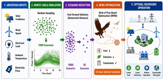
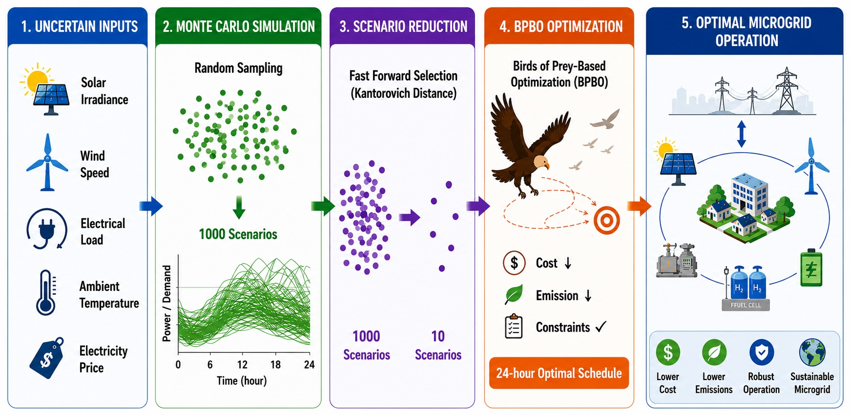
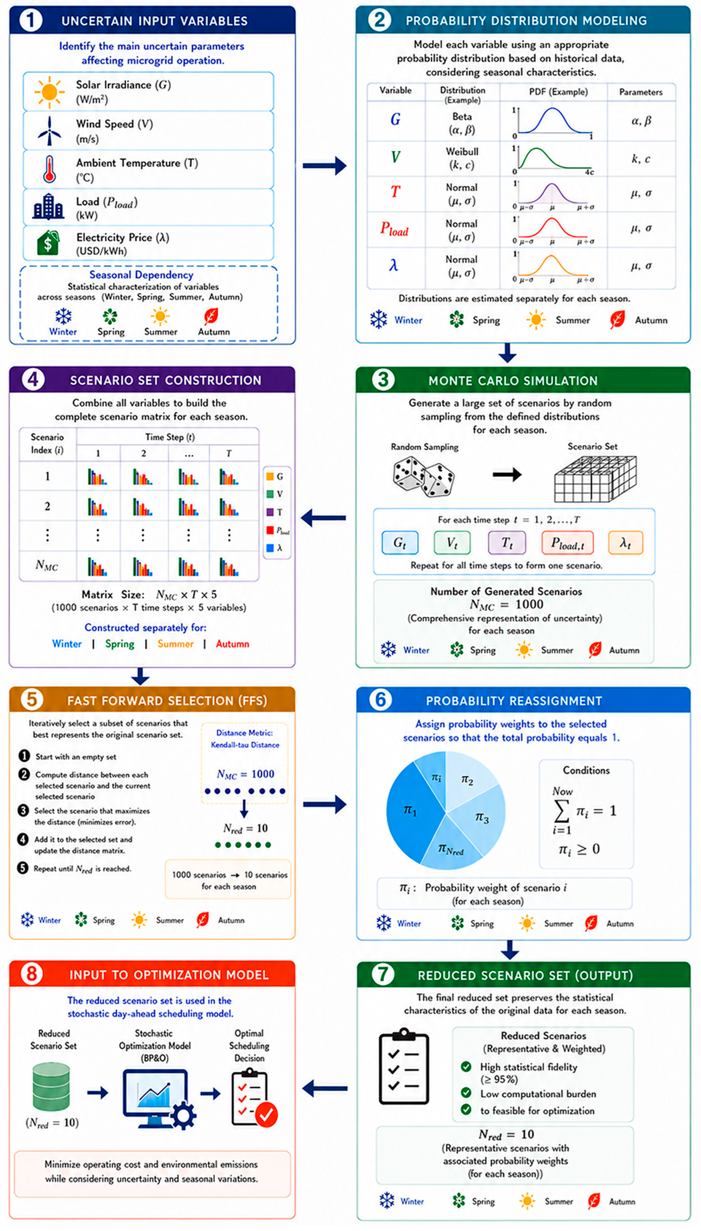
Representative scenarios	Reduce computational burden	10 scenarios selected from the original set	FFS using Kantorovich distance

. The seasonal input profiles provide the mean trajectories for uncertainty modeling, while the system-component parameters define the physical and economic limits of the MG scheduling problem. The complete data-preparation, scenario-generation, scenario-reduction, and optimization workflow is illustrated in Figure 2.

Using these inputs, 1000 MC scenarios are generated for each season. Each scenario contains a complete 24 h realization of solar irradiance, wind speed, ambient temperature, load demand, and electricity price. Since using all generated scenarios would significantly increase the computational burden, FFS based on Kantorovich distance is applied to obtain 10 representative scenarios. The reduced scenario set is then used in the BPBO-based day-ahead scheduling model.

The reduced representative scenario set is subsequently used within the BPBO-based day-ahead scheduling framework to determine the optimal coordinated operation of dispatchable generation units, ES charging/discharging actions, and utility-grid exchange under seasonal stochastic uncertainty.

4. Problem Formulation

The MG energy management problem seeks optimal dispatch schedules that minimize total operational costs while satisfying all technical and operational constraints. This formulation adopts a multi-objective approach, balancing economic efficiency against environmental sustainability.

4.1. Objective Function

The comprehensive multi-objective function incorporates both operational costs and emission penalties:

$$\mathrm{m}\mathrm{i}\mathrm{n} F=w_{\mathrm{cost}}·C_{\mathrm{op}}+w_{\mathrm{emission}}·C_{\mathrm{em}}$$

(25)

where $w_{\mathrm{cost}}$ and $w_{\mathrm{emission}}$ represent weighting factors for operational cost and emission cost, respectively, satisfying $w_{\mathrm{cost}}+w_{\mathrm{emission}}=1$.

The operational cost component aggregates fuel costs, grid transactions, and operation and maintenance expenses:

$$C_{\mathrm{op}}={\sum }_{t=1}^T\left[C_{\mathrm{MT}}\right(t)+C_{\mathrm{FC}}(t)+C_{\mathrm{grid}}(t)+C_{\mathrm{O}\&\mathrm{M}}(t\left)\right]\Delta t$$

(26)

where $C_{\mathrm{grid}}\left(t\right)$ represents the net grid cost given by

$$C_{\mathrm{grid}}\left(t\right)={\lambda }_{\mathrm{grid}}\left(t\right)·\left[P_{\mathrm{grid},\mathrm{buy}}\right(t)-P_{\mathrm{grid},\mathrm{sell}}(t\left)\right]$$

(27)

where ${\lambda }_{\mathrm{g}\mathrm{r}\mathrm{i}\mathrm{d}}\left(t\right)$ is the hourly electricity price, $P_{\mathrm{g}\mathrm{r}\mathrm{i}\mathrm{d},\mathrm{b}\mathrm{u}\mathrm{y}}\left(t\right)$ is the power purchased from the utility grid, and $P_{\mathrm{g}\mathrm{r}\mathrm{i}\mathrm{d},\mathrm{s}\mathrm{e}\mathrm{l}\mathrm{l}}\left(t\right)$ is the power sold to the utility grid. The hourly value of ${\lambda }_{\mathrm{g}\mathrm{r}\mathrm{i}\mathrm{d}}\left(t\right)$ represents the time-varying electricity price profile, so peak and off-peak tariff effects are included in the grid-exchange cost calculation.

The operation and maintenance cost encompasses contributions from all generation sources:

$$C_{\mathrm{O}\&\mathrm{M}}\left(t\right)={\gamma }_{\mathrm{MT}}{P}_{\mathrm{MT}}\left(t\right)+{\gamma }_{\mathrm{FC}}{P}_{\mathrm{FC}}\left(t\right)+{\gamma }_{\mathrm{PV}}{P}_{\mathrm{PV}}\left(t\right)+{\gamma }_{\mathrm{Wind}}{P}_{\mathrm{Wind}}\left(t\right)+{\gamma }_{\mathrm{ES}}{P}_{\mathrm{discharging}}\left(t\right)$$

(28)

where ${\gamma }_i$ denotes the operation and maintenance cost coefficient for the component $i$($/kWh).

Environmental impact quantification considers three major pollutants:

$$C_{\mathrm{em}}={\sum }_{t=1}^T\left[c_{{\mathrm{CO}}_2}{E}_{{\mathrm{CO}}_2}\right(t)+c_{{\mathrm{SO}}_2}{E}_{{\mathrm{SO}}_2}(t)+c_{{\mathrm{NO}}_x}{E}_{{\mathrm{NO}}_x}(t\left)\right]\Delta t$$

(29)

where $c_i$ represents the penalty cost for pollutant $i$ ($/kg), and emissions are calculated as

$$E_{{\mathrm{CO}}_2}(t)={\epsilon }_{\mathrm{MT}}^{{\mathrm{CO}}_2}{P}_{\mathrm{MT}}(t)+{\epsilon }_{\mathrm{FC}}^{{\mathrm{CO}}_2}{P}_{\mathrm{FC}}(t)+{\epsilon }_{\mathrm{grid}}^{{\mathrm{CO}}_2}{P}_{\mathrm{grid},\mathrm{buy}}(t)$$

(30)

$$E_{{\mathrm{SO}}_2}(t)={\epsilon }_{\mathrm{MT}}^{{\mathrm{SO}}_2}{P}_{\mathrm{MT}}(t)+{\epsilon }_{\mathrm{FC}}^{{\mathrm{SO}}_2}{P}_{\mathrm{FC}}(t)+{\epsilon }_{\mathrm{grid}}^{{\mathrm{SO}}_2}{P}_{\mathrm{grid},\mathrm{buy}}(t)$$

(31)

$$E_{{\mathrm{NO}}_x}(t)={\epsilon }_{\mathrm{MT}}^{{\mathrm{NO}}_x}{P}_{\mathrm{MT}}(t)+{\epsilon }_{\mathrm{FC}}^{{\mathrm{NO}}_x}{P}_{\mathrm{FC}}(t)+{\epsilon }_{\mathrm{grid}}^{{\mathrm{NO}}_x}{P}_{\mathrm{grid},\mathrm{buy}}(t)$$

(32)

where ${\epsilon }_j^i$ denotes the emission factor of pollutant $i$ from source $j$ (kg/kWh).

4.2. Operational Constraints

The optimization problem must satisfy multiple physical, technical, and operational constraints, ensuring feasible and safe system operation.

4.2.1. Power Balance Constraint

At each time interval, total generation must equal total consumption:

$$P_{\mathrm{MT}}\left(t\right)+P_{\mathrm{FC}}\left(t\right)+P_{\mathrm{PV}}\left(t\right)+P_{\mathrm{Wind}}\left(t\right)+P_{\mathrm{discharging}}\left(t\right)+P_{\mathrm{grid},\mathrm{buy}}\left(t\right)=P_{\mathrm{load}}\left(t\right)+P_{\mathrm{charging}}\left(t\right)+P_{\mathrm{grid},\mathrm{sell}}\left(t\right)$$

(33)

4.2.2. Generator Capacity Constraints

All generation units must operate within rated limits as follows:

• The MT output must respect technical constraints:

$$P_{\mathrm{MT}}^{\mathrm{m}\mathrm{i}\mathrm{n}}\le P_{\mathrm{MT}}\left(t\right)\le P_{\mathrm{MT}}^{\mathrm{m}\mathrm{a}\mathrm{x}}$$

(34)

where $P_{\mathrm{MT}}^{\mathrm{m}\mathrm{i}\mathrm{n}}$ and $P_{\mathrm{MT}}^{\mathrm{m}\mathrm{a}\mathrm{x}}$ define the minimum and maximum generation limits (kW), respectively.

• Operating limits constrain the FC output:

$$P_{\mathrm{FC}}^{\mathrm{m}\mathrm{i}\mathrm{n}}\le P_{\mathrm{FC}}\left(t\right)\le P_{\mathrm{FC}}^{\mathrm{m}\mathrm{a}\mathrm{x}}$$

(35)

where $P_{\mathrm{FC}}^{\mathrm{m}\mathrm{i}\mathrm{n}}$ and $P_{\mathrm{FC}}^{\mathrm{m}\mathrm{a}\mathrm{x}}$ define the minimum and maximum generation limits of FC (kW), respectively.

• PV Power output bounds:

$$0\le P_{\mathrm{PV}}\left(t\right)\le P_{\mathrm{PV}}^{\mathrm{available}}\left(t\right)$$

(36)

where $P_{\mathrm{PV}}$(t) is the dispatched PV power at hour t. $P_{\mathrm{PV}}^{\mathrm{available}}$ represents the available PV power at hour $t$, calculated from the corresponding solar irradiance model. Thus, the PV generation limits vary over the 24 h scheduling horizon and across different stochastic scenarios.

• Wind generation bounds:

$$0\le P_{\mathrm{wind}}\left(t\right)\le P_{\mathrm{wind}}^{\mathrm{available}}\left(t\right)$$

(37)

where $P_{\mathrm{wind}}\left(t\right)$ is the dispatched wind power at the hour $t$. $P_{\mathrm{wind}}^{\mathrm{available}}\left(t\right)$ represents the available wind power at hour $t$, calculated from the corresponding wind-speed model. Thus, the wind generation limits vary over the 24 h scheduling horizon and across different stochastic scenarios.

4.2.3. Energy Storage Constraints

ES operation respects SOC limits, power limits, and charging/discharging exclusivity can be formulated as follows:

$${\mathrm{SOC}}^{\mathrm{m}\mathrm{i}\mathrm{n}}\le \mathrm{SOC}\left(t\right)\le {\mathrm{SOC}}^{\mathrm{m}\mathrm{a}\mathrm{x}}$$

(38)

where ${\mathrm{SOC}}^{\mathrm{m}\mathrm{i}\mathrm{n}}$ is the minimum allowable SOC, and ${\mathrm{SOC}}^{\mathrm{m}\mathrm{a}\mathrm{x}}$ is the maximum allowable SOC. The lower limit ${\mathrm{SOC}}^{\mathrm{m}\mathrm{i}\mathrm{n}}$ prevents deep discharge, while the upper limit ${\mathrm{SOC}}^{\mathrm{m}\mathrm{a}\mathrm{x}}$ prevents excessive charging. In this study, the ES is maintained within the allowable SOC range of 15–95% [24]. The lower SOC limit prevents deep discharge and excessive battery stress, while the upper SOC limit avoids overcharging conditions that may negatively affect battery lifetime and operational safety.

$$0\le P_{\mathrm{charging}}\left(t\right)\le P_{\mathrm{charging}}^{\mathrm{m}\mathrm{a}\mathrm{x}}$$

(39)

$$0\le P_{\mathrm{discharging}}\left(t\right)\le P_{\mathrm{discharging}}^{\mathrm{m}\mathrm{a}\mathrm{x}}$$

(40)

$$P_{\mathrm{charging}}\left(t\right)·P_{\mathrm{discharging}}\left(t\right)=0$$

(41)

where the final constraint prevents simultaneous charging and discharging.

To ensure battery longevity and operational continuity, the final SOC should return to its initial value:

$$\mathrm{S}\mathrm{O}\mathrm{C}\left(T\right)=\mathrm{S}\mathrm{O}\mathrm{C}\left(0\right)$$

(42)

These constraints ensure that the ES supports MG operation while avoiding harmful deep-discharge or overcharge conditions.

4.2.4. Load Constraints

To ensure physical consistency, each generated load-demand scenario is constrained as:

$$P_L^{\mathrm{m}\mathrm{i}\mathrm{n}}\left(t\right)\le P_{L,s}\left(t\right)\le P_L^{\mathrm{m}\mathrm{a}\mathrm{x}}\left(t\right)$$

(43)

where $P_{L,s}\left(t\right)$ is the generated load demand for scenario $s$ at hour $t$, $P_L^{\mathrm{m}\mathrm{i}\mathrm{n}}\left(t\right)>0$ is the minimum allowable load demand, and $P_L^{\mathrm{m}\mathrm{a}\mathrm{x}}\left(t\right)$ is the maximum allowable load demand. This bounded treatment avoids negative demand values while preserving the assumed short-term stochastic variation around the seasonal hourly mean load.

4.2.5. Grid Exchange Constraints

Power transactions with the grid remain within contracted limits and prevent simultaneous buying and selling can be defined as follows:

$$0\le P_{\mathrm{grid},\mathrm{buy}}(t)\le P_{\mathrm{grid}}^{\mathrm{m}\mathrm{a}\mathrm{x},\mathrm{buy}}$$

(44)

$$0\le P_{\mathrm{grid},\mathrm{sell}}(t)\le P_{\mathrm{grid}}^{\mathrm{m}\mathrm{a}\mathrm{x},\mathrm{sell}}$$

(45)

$$P_{\mathrm{grid},\mathrm{buy}}\left(t\right)·P_{\mathrm{grid},\mathrm{sell}}\left(t\right)=0$$

(46)

where $P_{\mathrm{grid},\mathrm{buy}}\left(t\right)$ and $P_{\mathrm{grid},\mathrm{sell}}\left(t\right)$ represent grid purchase and sale powers (kW), while $P_{\mathrm{grid}}^{\mathrm{m}\mathrm{a}\mathrm{x},\mathrm{buy}}$ and $P_{\mathrm{grid}}^{\mathrm{m}\mathrm{a}\mathrm{x},\mathrm{sell}}$ denote maximum exchange limits (kW).

5. Birds of Prey-Based Optimizer

5.1. Inspiration

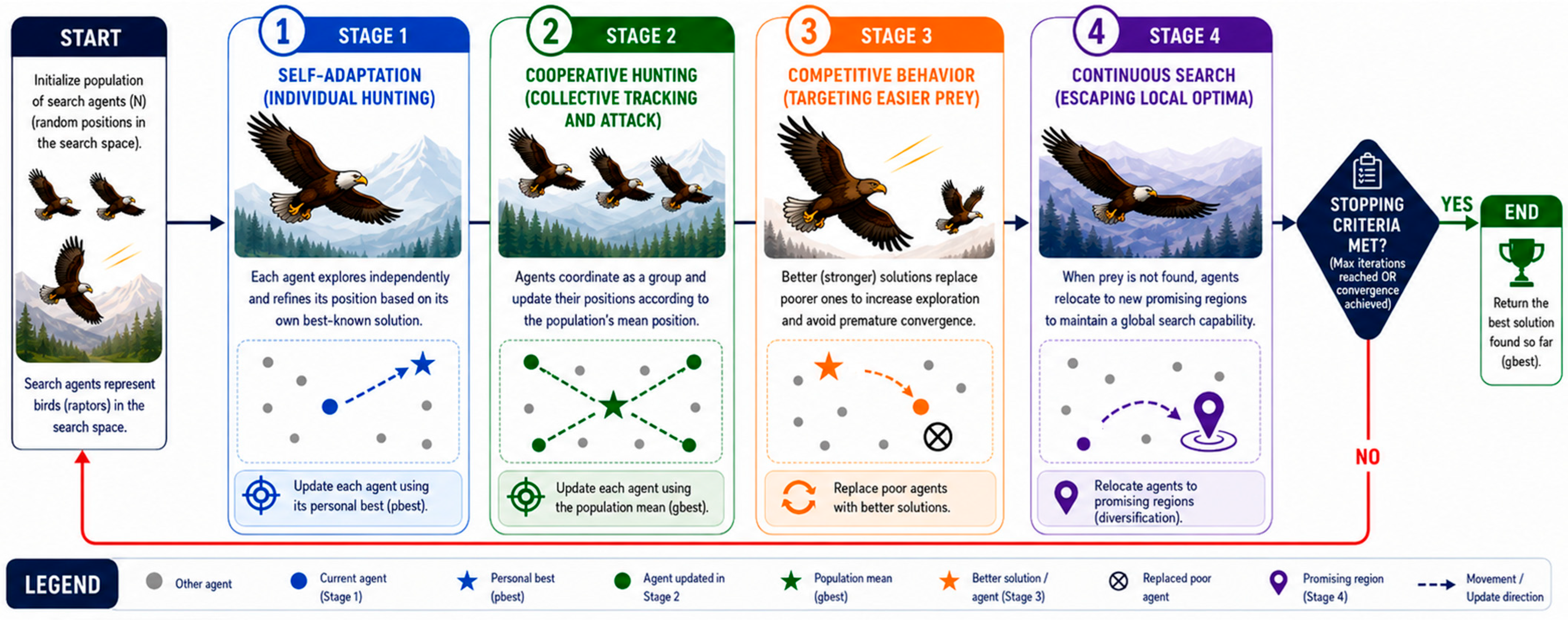
The proposed BPBO algorithm is inspired by the multifaceted hunting behaviors observed in birds of prey. These raptors employ both solitary and cooperative strategies, while also facing the risk of becoming prey themselves. At times, a hunting bird may fail to secure its target, prompting it to continue searching and adjusting its strategy. The proposed optimizer models these natural behaviors by translating them into a structured optimization model composed of four main stages, as displayed in Figure 3, each representing a specific type of avian hunting action:

• Stage #1: Self-adaptation (individual hunting): Raptors such as eagles and falcons rely heavily on speed, agility, and independent decision-making when pursuing prey. In the algorithm, this behavior is reflected through individual exploration and refinement, where each search agent updates its position based on its best-identified solution, much like a bird adjusting its trajectory to reach food more efficiently.
• Stage #2: Cooperative hunting (collective tracking and attack): Species like kites and hawks often hunt in coordinated groups, synchronizing their movements to overwhelm prey. The BPBO framework mimics this through population-based adjustments, where agents update their trajectories according to the group’s mean position, increasing diversity and strengthening the collective search capability.
• Stage #3: Competitive behavior (targeting easier prey): In nature, stronger raptors may pursue smaller or weaker birds when an opportunity arises. This competitive instinct is modeled by allowing superior solutions to replace poorer ones, which increases the exploration potential of the algorithm and helps avoid premature convergence.
• Stage #4: Continuous search (escaping local optima): When prey is not found, birds naturally relocate to new grounds. To emulate this, the developed method incorporates a relocation mechanism that directs agents toward promising regions, ensuring that the global search process remains active and dynamic.

5.2. Optimization Process

By aligning each procedural step with specific avian behaviors, the BPBO algorithm maintains a balanced interplay between exploitation and exploration, ultimately improving its optimization performance. The process of implementing the proposed algorithm can be summarized as follows:

Step #1: Initialization of the BPBO population

As with most meta-heuristic methods, the procedure begins by generating an initial set of (N) candidate solutions within the search space (analogous to a hunting field). The best individual, denoted as ($G_{best}$ or prey), represents the prey as $X_{pray}$, while the remaining (N − 1) individuals act as hunters. For each agent (i = 1:N), the initial position is assigned according to:

$$X_i=X_{min}+rand(1,D)\times (X_{max}-X_{min})$$

(47)

where the maximum and minimum ranges of decisions are defined by the upper and lower bounds of decision variables $X_{max} and X_{min}$, D is the dimensionality of the problem, and rand generates uniformly distributed random numbers in [0, 1].

Step #2: Identifying the raptor

Once the population is initialized, exploration begins. Similar to how raptors continually scan their surroundings for suitable prey, each agent begins seeking its objective, denoted as $P_i$. This marks the start of the search process, leading to the behaviors described in Steps 3 to 5.

Step #3: Individual hunting

During this stage, each hunter, $X_i$, attempts to close the distance to the current prey $X_{pray}$, which represents the best solution found so far. The agent updates its position by integrating information from the optimal solution, thereby refining its approach toward the global optimum. The update rule is:

$$X_i^{new}=X_i+rand(1,D)\times (X_{prey}-K_{i1}\times X_i)$$

(48)

where $K_{i1}$ = 1 or 2, which randomly determines whether the hunter approaches the target from the front or the rear.

Step #4: Group hunting

In many species, birds of prey combine individual and collective hunting. Within BPBO, the population forms a collective center given by the mean position $X_{mean}$. Agents then align themselves either individually or cooperatively toward $X_{prey}$. This group-enhanced movement is modeled by:

$$X_i^{new}=X_{mean}+rand(1,D)\times (X_{prey}-K_{i2}\times X_{mean})$$

(49)

where $K_{i2}$ = 1 or 2, which randomly determines the direction of attack relative to the prey.

Step #5: Targeting weaker prey (competition)

Raptors sometimes pursue smaller or weaker birds to secure an easy meal. The algorithm captures this competitive mechanism by allowing hunters to adjust their positions relative to the weakest individual, $X_{Worst}$:

$$X_i^{new}=X_i+rand(1,D)\times (X_i-K_{i3}\times X_{Worst})$$

(50)

where $K_{i3}$ = 1 or 2, which indicates whether the attack is from the front or the back. This mechanism enhances diversity and prevents stagnation.

Step #6: Continued search

If a particular agent fails to locate suitable prey during iteration ith, it relocates to explore new areas of the search space. This is expressed as:

$$X_i^{new}=X_i+{rand}_1\times X_{min}+rand\times (X_{max}-X_{min})$$

(51)

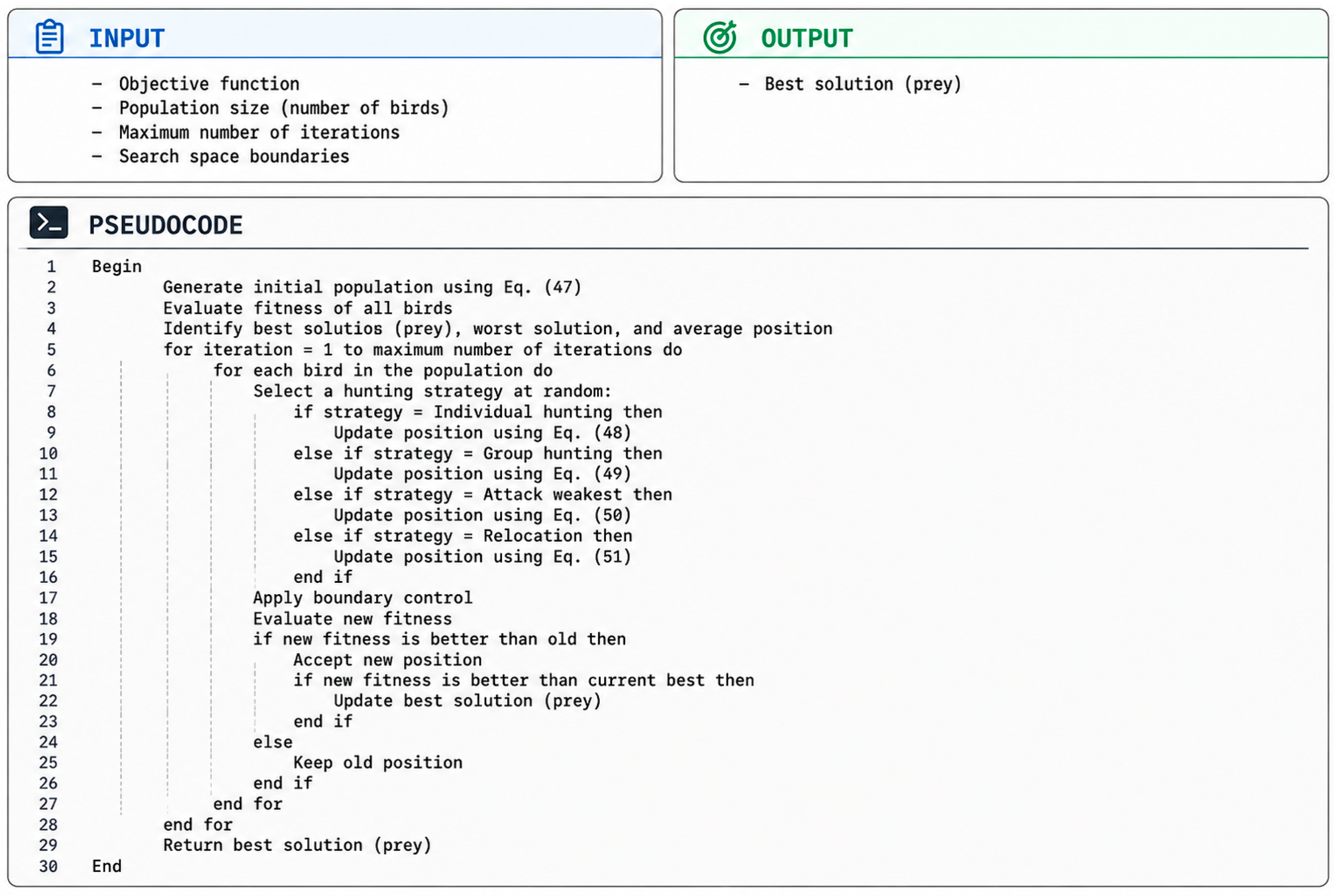
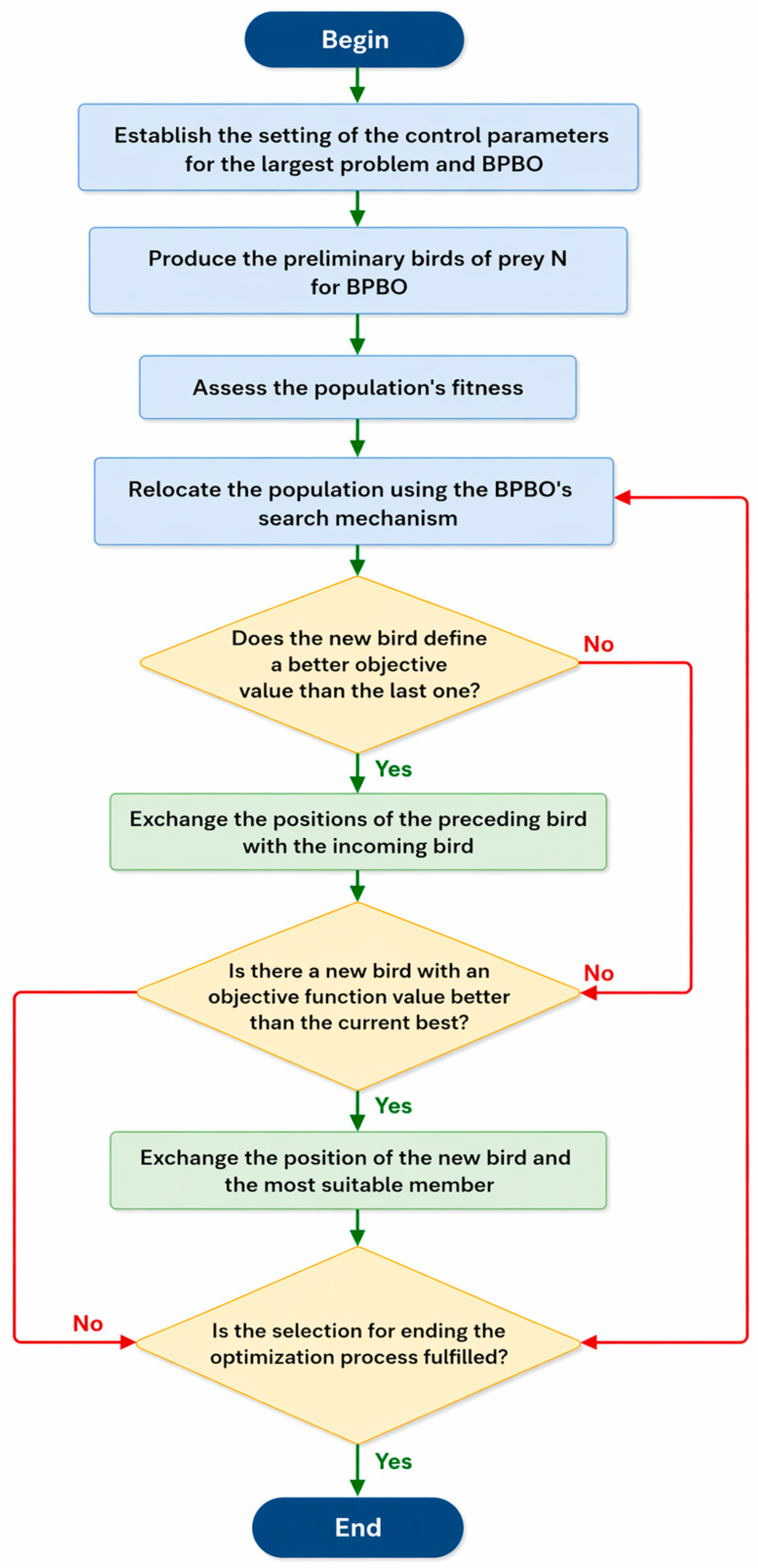
where ${rand}_1$ is a random number in the range 0 to 1, and each phase described occurs probabilistically. Finally, Figure 4 and Figure 5 illustrate the pseudocode and the overall optimization workflow.

5.3. BPBO Application to the MG Scheduling Problem

In this study, the BPBO algorithm is applied to solve the stochastic day-ahead scheduling problem of the grid-connected multi-energy MG. Unlike a generic optimization description, each BPBO search agent represents a complete candidate dispatch schedule for the controllable power-system components over the 24 h scheduling horizon.

For the $i$-th search agent, the decision vector is defined as:

$$\begin{gathered} {\mathrm{X}}_i=\left[P_{\mathrm{M}\mathrm{T},i}\left(1:T\right),P_{\mathrm{F}\mathrm{C},i}\left(1:T\right),P_{\mathrm{c}\mathrm{h}\mathrm{a}\mathrm{r}\mathrm{g}\mathrm{i}\mathrm{n}\mathrm{g},i}\left(1:T\right),P_{\mathrm{d}\mathrm{i}\mathrm{s}\mathrm{c}\mathrm{h}\mathrm{a}\mathrm{r}\mathrm{g}\mathrm{i}\mathrm{n}\mathrm{g},i}\left(1:T\right),P_{\mathrm{g}\mathrm{r}\mathrm{i}\mathrm{d},\mathrm{b}\mathrm{u}\mathrm{y},i}\left(1:T\right),P_{\mathrm{g}\mathrm{r}\mathrm{i}\mathrm{d},\mathrm{s}\mathrm{e}\mathrm{l}\mathrm{l},i}\left(1:T\right)\right], \\ T=24 \end{gathered}$$

(52)

where $P_{\mathrm{M}\mathrm{T},i}(1:T)$ and $P_{\mathrm{F}\mathrm{C},i}(1:T)$ are the 24 h scheduled power outputs of the MT and FC, respectively. $P_{\mathrm{c}\mathrm{h}\mathrm{a}\mathrm{r}\mathrm{g}\mathrm{i}\mathrm{n}\mathrm{g},i}(1:T)$ and $P_{\mathrm{d}\mathrm{i}\mathrm{s}\mathrm{c}\mathrm{h}\mathrm{a}\mathrm{r}\mathrm{g}\mathrm{i}\mathrm{n}\mathrm{g},i}(1:T)$ are the 24 h ES charging and discharging power schedules, while $P_{\mathrm{g}\mathrm{r}\mathrm{i}\mathrm{d},\mathrm{b}\mathrm{u}\mathrm{y},i}(1:T)$ and $P_{\mathrm{g}\mathrm{r}\mathrm{i}\mathrm{d},\mathrm{s}\mathrm{e}\mathrm{l}\mathrm{l},i}(1:T)$ are the 24 h grid purchase and sale power schedules. Therefore, each candidate solution contains six hourly control-variable groups over the 24 h scheduling horizon, resulting in $6\times 24=144$ decision variables.

PV and wind generations are not treated as independent BPBO decision variables in this formulation. Instead, $P_{PV}\left(t\right)$ and $P_{WT}\left(t\right)$ are calculated from the hourly solar-irradiance and wind-speed scenarios, respectively. These renewable-generation values are incorporated into the power-balance equation as time-dependent available generation and are constrained by their corresponding hourly maximum available power limits.

For each representative scenario, the candidate dispatch schedule is evaluated using the proposed cost–emission fitness function. The fitness value of the $i$-th search agent is expressed as:

$$F_i=w_{\mathrm{c}\mathrm{o}\mathrm{s}\mathrm{t}}{C}_{\mathrm{o}\mathrm{p},i}+w_{\mathrm{e}\mathrm{m}\mathrm{i}\mathrm{s}\mathrm{s}\mathrm{i}\mathrm{o}\mathrm{n}}{C}_{\mathrm{e}\mathrm{m},i}$$

(53)

where $C_{op,i}$ represents the operating cost, $C_{em,i}$ denotes the emission cost, and $w_{cost}$ and $w_{emission}$ are the corresponding weighting coefficients. In the stochastic scheduling framework, these costs are evaluated over the reduced representative scenario set obtained from the FFS procedure.

The main constraints checked during the evaluation process include the power-balance constraint, MT and FC generation limits, ES charging/discharging limits, SOC limits, cyclic final SOC condition, grid purchase/sale limits, and time-dependent PV and wind availability constraints.

During the BPBO search process, each candidate dispatch schedule is updated through the individual-hunting, cooperative-hunting, competition, and continued-search mechanisms of the algorithm. After each update, the candidate solution is verified against the operating limits of the MG components. If any variable exceeds its allowable operating range, it is corrected to the nearest feasible bound. Subsequently, the ES SOC trajectory is recalculated over the 24 h scheduling horizon to ensure that the ES remains within the allowable SOC limits.

Finally, the best candidate solution is selected according to the minimum expected fitness value over the reduced representative scenario set. Therefore, the BPBO algorithm is directly linked to the MG scheduling variables and is effectively used to coordinate dispatchable generation, ES operation, and utility-grid exchange under seasonal stochastic uncertainty.

6. Results and Discussion

The optimization of MG energy management systems under stochastic renewable generation and seasonal demand variations represents a critical challenge in modern power systems. To evaluate the realism of the adopted uncertainty-modeling framework, the generated stochastic scenarios were compared with the corresponding hourly seasonal mean profiles used during the MC scenario-generation stage. The generated renewable-generation, load-demand, ambient-temperature, and electricity price trajectories remained physically consistent with expected real-time MG operating behavior. In particular, solar irradiance scenarios maintained zero nighttime generation and realistic daytime peaks, wind-speed scenarios remained within turbine operating limits, and electrical-load scenarios preserved practical hourly demand variations without generating nonphysical values. Similarly, the generated electricity price scenarios successfully reflected peak and off-peak tariff behavior over the 24 h scheduling horizon. These observations confirm that the adopted probabilistic uncertainty models and MC-based scenario-generation framework provide realistic seasonal operating scenarios suitable for stochastic MG scheduling analysis.

This study proposes the BPBO algorithm as an efficient solution methodology and validates its effectiveness through a comprehensive comparison with five established metaheuristic algorithms, PSO [30], DE [31], ALO [32], DO [33], and ACO [34]. The benchmark algorithms used in this study are selected to represent different metaheuristic search mechanisms and to provide a balanced comparison with the proposed BPBO method. PSO is included as a representative swarm-intelligence optimizer based on velocity-guided social learning. DE is selected as an evolutionary algorithm based on mutation, recombination, and selection. ALO is used to represent random-walk-based exploration and exploitation, while ACO is included as a pheromone-guided constructive search method. DO is also considered because it represents a more recent seed-dispersal-based population optimizer. This set of algorithms allows BPBO to be evaluated against optimizers with different search behaviors, convergence characteristics, and population-update mechanisms. Other recent metaheuristics, such as Harris Hawks Optimization, Whale Optimization Algorithm, Marine Predators Algorithm, and Grey Wolf Optimizer, are also relevant for MG scheduling; however, they are not included in the present comparison to keep the computational study focused across four seasonal cases, 30 independent runs with 100 maximum iterations, and stochastic scenario-based optimization. A broader comparison with these recent algorithms will be considered in future work to further assess the relative performance and scalability of BPBO. The investigation addresses optimal energy dispatch for a grid-connected MG incorporating PV arrays, WTs, MT, FC, ES, and grid connection under realistic season-dependent behavior.

Table 4. Main BPBO parameter settings used in the simulation.

Parameter	Description	Value Used
Number of runs	Independent optimization trials	30
$\mathit{N}$	Population size	30
${\mathit{i}\mathit{t}\mathit{e}\mathit{r}}_{\mathbf{m}\mathbf{a}\mathbf{x}}$	Maximum number of iterations	100
$\mathit{D}$	Number of decision variables	6 $\times$ 24 = 144
${\mathit{X}}_{\mathbf{m}\mathbf{i}\mathbf{n}}$	Lower bound of decision variables	Component-dependent
${\mathit{X}}_{\mathbf{m}\mathbf{a}\mathbf{x}}$	Upper bound of decision variables	Component-dependent
${\mathit{K}}_{\mathit{i}1}$, ${\mathit{K}}_{\mathit{i}2}$, ${\mathit{K}}_{\mathit{i}3}$	Randomly determines the direction of attack	1 or 2

lists the main BPBO parameter settings used in the simulation. The multi-objective fitness function simultaneously minimizes both operational costs and pollutant-related costs, weighed equally at 50% each, thereby achieving a balanced economic–environmental scheduling strategy.

6.1. Seasonal Energy Profile Characteristics

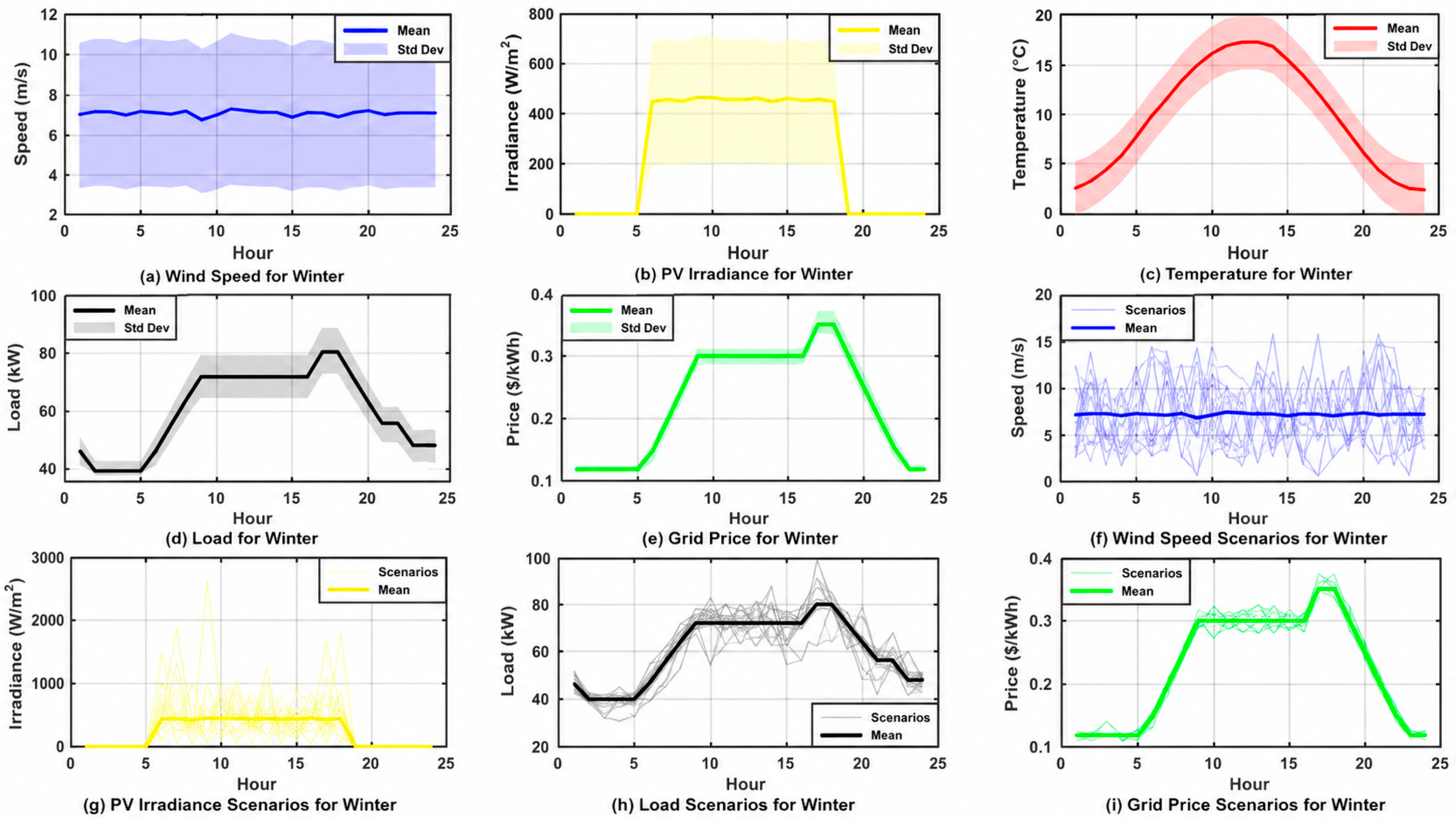
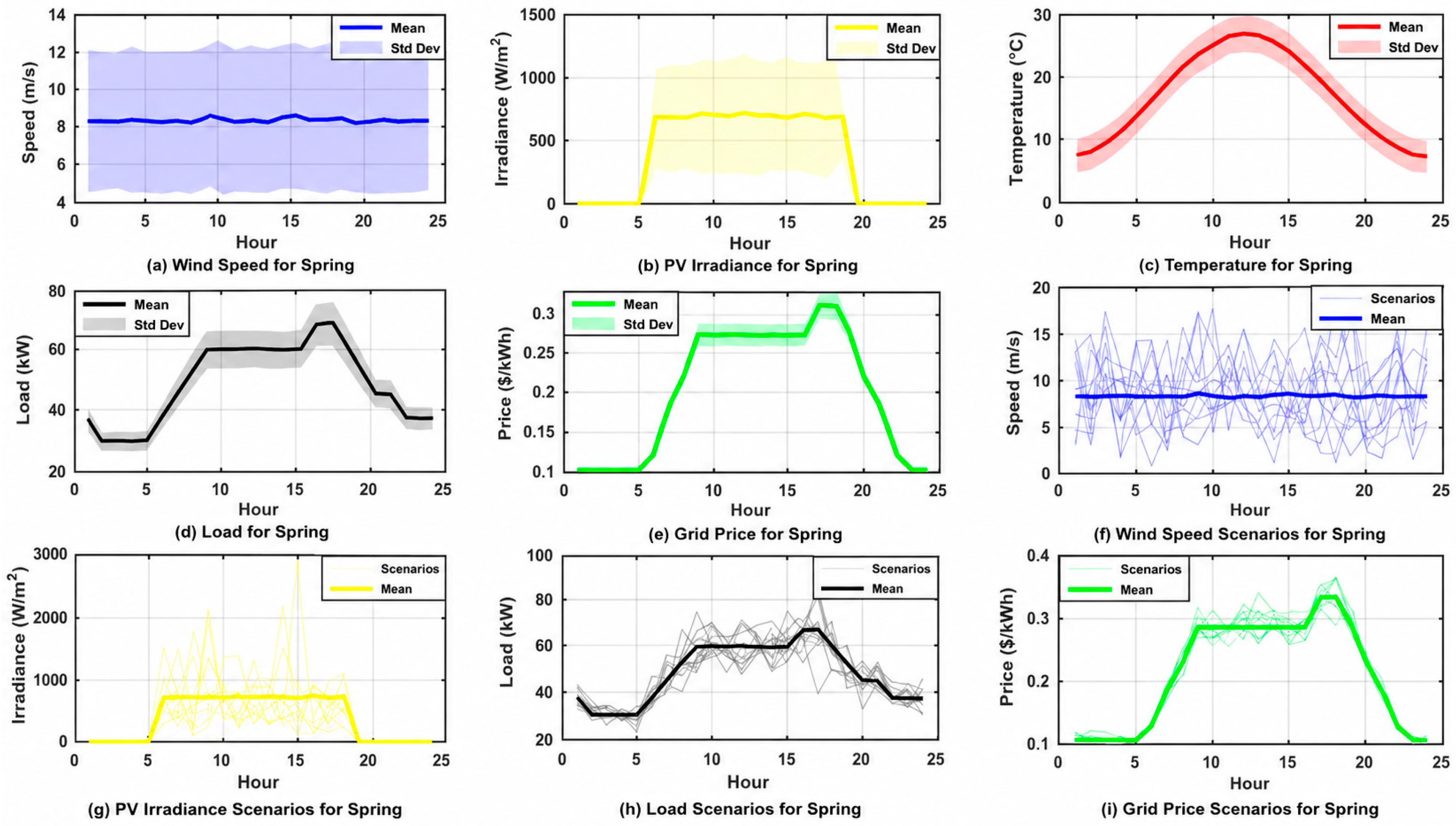
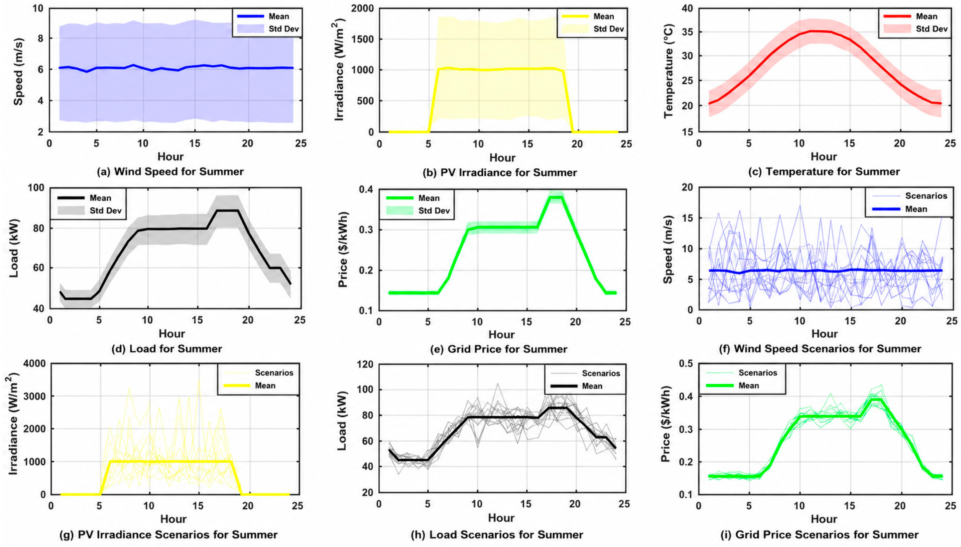
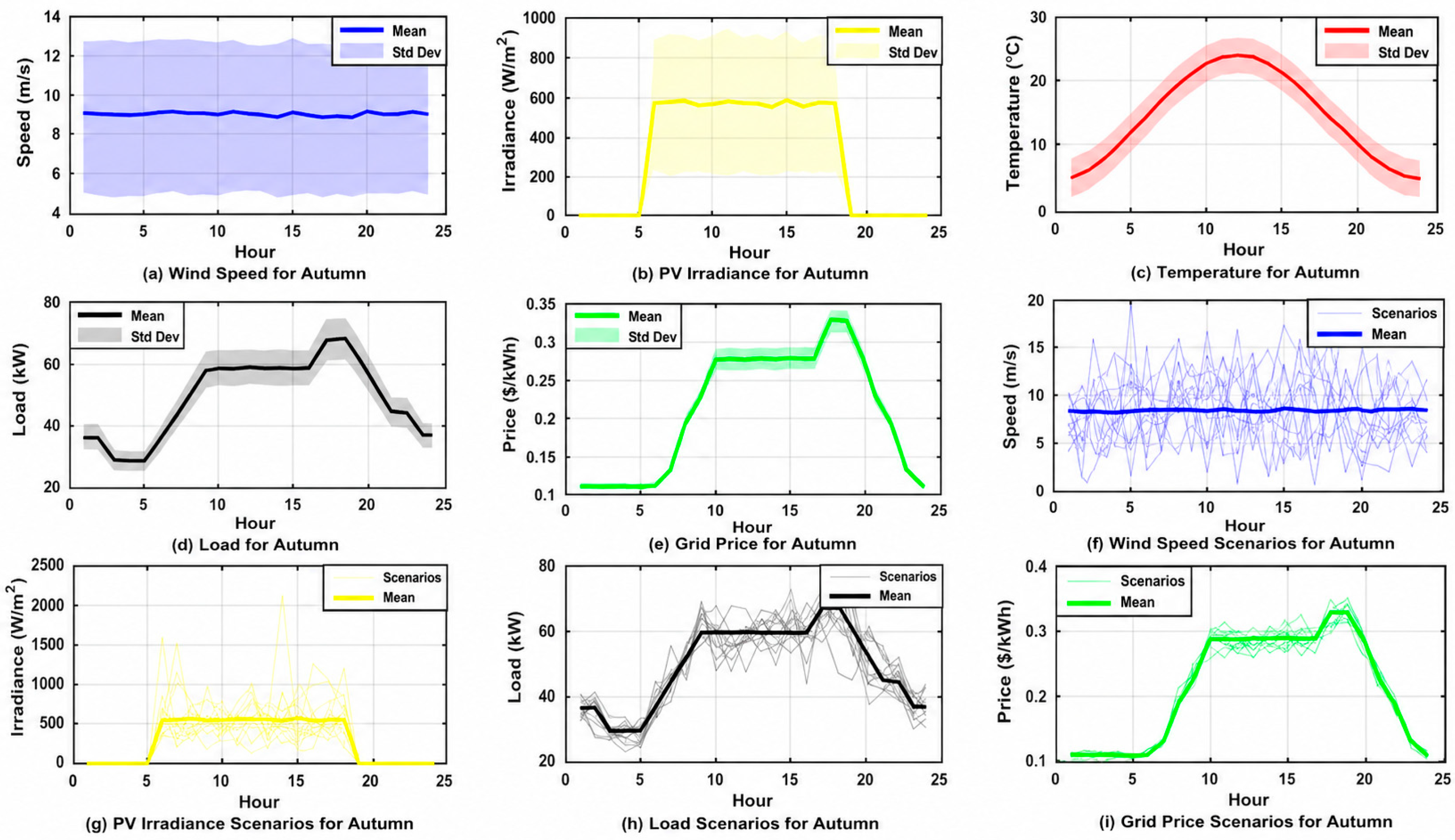
The generated data profiles reveal distinct seasonal patterns that fundamentally influence optimization outcomes. Figure 6, Figure 7, Figure 8 and Figure 9 demonstrate substantial variations in solar irradiance, wind speed, ambient temperature, and load demand across winter, spring, summer, and autumn seasons. Winter conditions (Figure 6) exhibit reduced PV generation capacity due to lower solar irradiance levels, coupled with moderate wind availability and elevated heating loads during early morning and evening hours. Conversely, spring conditions (Figure 7) show increased solar potential with balanced wind resources and moderate load profiles. Summer (Figure 8) presents the highest PV generation potential but also encounters peak cooling loads during midday and afternoon periods, creating critical demand windows. Autumn (Figure 9) demonstrates transitional characteristics with enhanced wind generation compensating for declining solar availability.

These substantial climatic effects directly impact optimization complexity and solution characteristics. Summer’s high load-to-generation ratio necessitates maximum utilization of dispatchable resources and continuous grid imports, constraining solution flexibility. Conversely, spring’s balanced supply–demand relationship enables diverse dispatch strategies, testing the optimizer’s ability to identify economically optimal resource allocation patterns. The stochastic modeling approach, incorporating MC simulation with Beta-distributed solar irradiance and Weibull-distributed wind speed, accurately captures real-world uncertainty that BPBO must navigate to identify robust operational strategies. The implementation of scenario reduction techniques ensures computational tractability while preserving statistical fidelity of the uncertainty representation.

6.2. Optimal Power Dispatch Across Seasons

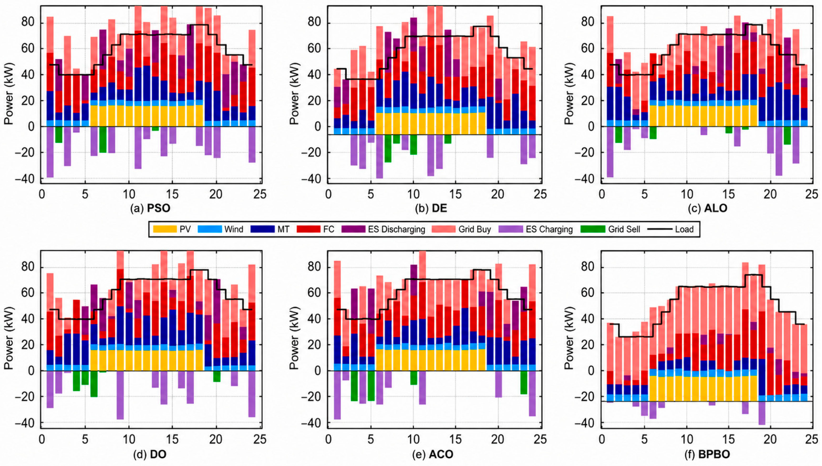
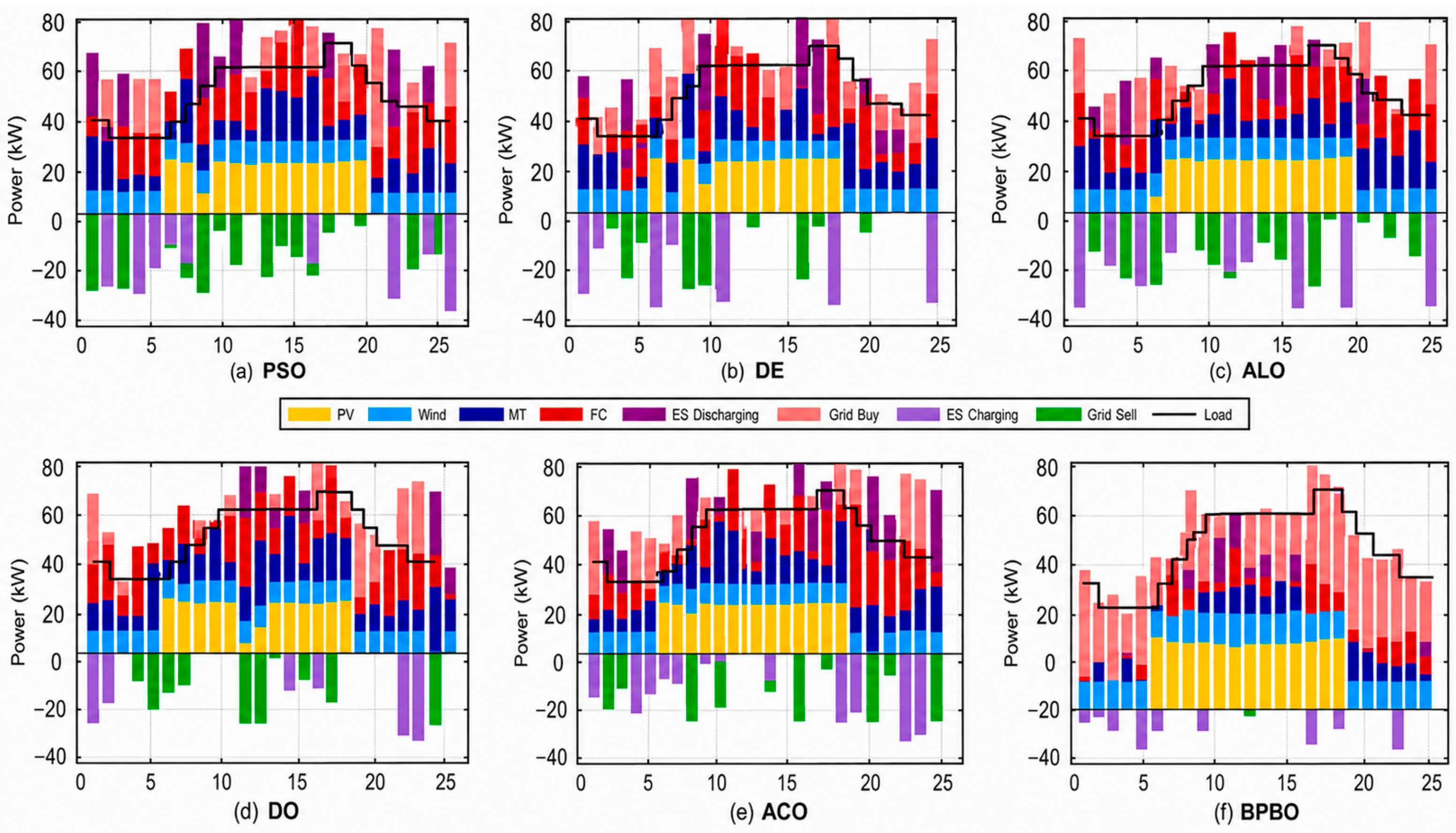
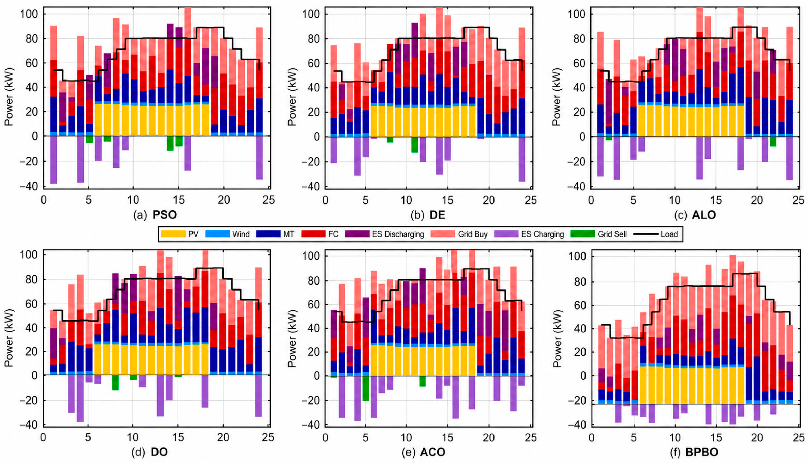
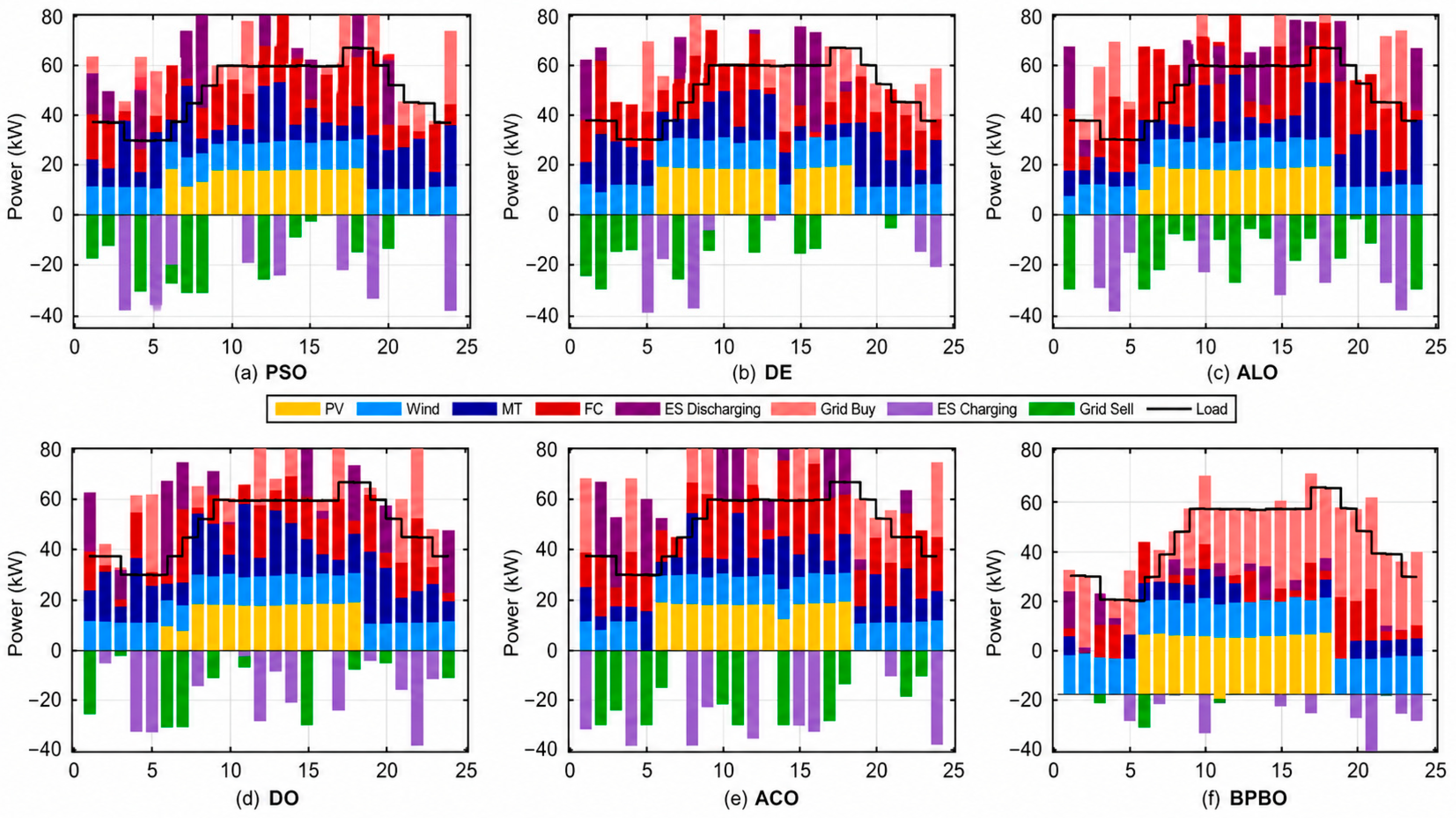
The hourly power scheduling results for all four seasons using the BPBO optimizer are visualized through stacked bar charts in Figure 10, Figure 11, Figure 12 and Figure 13. These results demonstrate the algorithm’s capability to orchestrate diverse distributed energy resources while satisfying complex operational constraints, including power balance, ES state-of-charge limits, and component capacity restrictions.

6.2.1. Winter Season Dispatch Strategy

Figure 10 illustrates the optimal 24 h power scheduling for the winter season. During nighttime hours (hours 1–5 and 19–24) when solar generation is unavailable, the system exhibits a coordinated dispatch pattern that leverages the MT operating consistently at or near its minimum power threshold of 6 kW to ensure technical feasibility. Grid imports reach the maximum allowable limit of 30 kW during peak demand periods (hours 1, 5–10, 12–19, and 22–24), indicating the grid serves as the primary balanced resource when renewable generation is insufficient. The FC operates flexibly across a wide power range, from zero to 30 kW, responding dynamically to load variations and complementing other generation sources. Wind power maintains relatively steady contributions ranging from 3.83 to 4.83 kW throughout the day, reflecting the moderate wind conditions characteristic of winter meteorology in the study region.

The PV system delivers its peak generation of approximately 15–16 kW during midday hours (6–18), coinciding with maximum solar irradiance. This substantial solar contribution during daylight hours enables strategic ES charging operations, with notable charging events occurring at hours 1, 2, 4, 5, 6, 7, and 17–19, storing energy when generation capacity exceeds immediate demand or when electricity prices are favorable. Conversely, ES discharging events at hours 3, 8, 9, 12, 14–16, 18, and 20–24 provide critical load support during high-demand periods or when marginal generation costs exceed ES discharge costs. The ES management strategy successfully maintains SOC within prescribed limits (20–90%) while returning to the initial 50% SOC at hour 24, ensuring daily cyclic operation without long-term degradation. Notably, no grid sales occur during winter, as the relatively low renewable penetration combined with higher heating loads results in consistent net energy import from the grid.

Although local sources are available in the studied MG, the optimized schedule may still select grid purchase during some hours. This behavior occurs because the objective function minimizes the total operating and emission costs rather than minimizing grid import alone. Therefore, the grid can be used when its hourly electricity price is economically favorable or when increasing local dispatchable generation would produce a higher total cost or emission penalty.

In winter, the grid-use pattern is affected by the combined influence of renewable availability, load demand, SOC limits, and MT/FC operating constraints. During hours when renewable generation is not sufficient or when the ES must preserve its SOC for later high-demand periods, grid purchase can become the most suitable balancing source. Thus, higher grid use in certain hours does not indicate an optimization error. Instead, it reflects the cost–emission trade-off selected by the optimizer under the imposed operational constraints.

6.2.2. Spring Season Operating Schedule

The spring season results, visualized in Figure 11, reveal a markedly different operational paradigm characterized by enhanced renewable energy availability and moderate load profiles. Wind power generation increases significantly compared to winter, ranging from 7.24 to 9.84 kW, nearly doubling the winter baseline. This higher wind capacity factor stems from the stronger spring winds prevalent in the geographical location under study. Solar generation exhibits even more pronounced enhancement, with PV output reaching 20–22 kW during peak irradiance hours (6–18), representing approximately 30–40% improvement over winter conditions. This increased solar yield results from longer daylight duration, reduced atmospheric attenuation, and optimal solar panel operating temperatures during the spring months.

The abundance of renewable generation fundamentally alters the dispatch logic. Grid imports decrease substantially, with several hours (11 and 17) requiring minimal or zero grid imports. The system even achieves net export conditions at hour 11, selling 1.17 kW back to the grid, a capability absent during winter operation. This demonstrates the season’s superior renewable resource availability, enabling occasional grid support rather than continuous dependence. MT and FC utilization become more selective, with multiple hours showing zero conventional generation as renewables and ES sufficiently meet demand. ES charging activities intensify during high solar production periods (hours 1, 2, 3, 5, 6, 9, 16, 18, and 22), accumulating surplus renewable energy. Strategic discharge events (hours 8, 10, 11, 13, 15, and 20) provide seamless load support during transient demand peaks or renewable generation dips. The coordinated renewable–ES-grid interaction exemplifies the spring season’s favorable energy economics, reducing reliance on fossil-fueled generation and associated emissions.

6.2.3. Summer Season Dispatch Pattern

Summer presents the most challenging operational scenario, as evidenced by Figure 12. The seasonal load profile peaks at 90.20 kW (hour 19), representing the highest demand across all seasons due to intensive air conditioning requirements in hot climates. This 25–30% increase compared to spring and autumn significantly stresses the MG’s generation portfolio. Despite enhanced solar availability, PV generation reaches 24–25 kW during hours 6–18, and the massive cooling loads necessitate maximum utilization of all available resources. The MT and FC frequently operate at their rated capacities of 30 kW during afternoon and evening peak periods (hours 10, 11, 14, and 16–20), unlike the part-load operation observed in other seasons.

Grid imports remain at the maximum 30 kW threshold for most hours, particularly during the critical peak demand window (hours 8–19). Wind generation declines to approximately 1.81–2.65 kW, substantially lower than spring and autumn, reflecting typical summer wind patterns characterized by calm conditions. This wind scarcity exacerbates the supply–demand imbalance. The ES operates under high stress, executing frequent charging (hours 3, 4, 5, 7, 10, 14, and 16) and discharging (hours 1, 2, 8, 9, 12, 13, 15, 19, 21, 23, and 24) cycles to provide rapid response capability. Despite these intensive dispatch strategies, the system never achieves surplus conditions suitable for grid exports, underscoring the summer’s net energy deficit characteristic. The summer scenario thus validates the robustness of the energy management approach under extreme loading conditions where conventional generation, renewables, storage, and grid support must synergistically operate at near-maximum capacity.

6.2.4. Autumn Season Dispatch Strategy

Autumn operational characteristics, presented in Figure 13, closely resemble spring patterns with minor variations. Wind power generation averages 10.83–12.23 kW, representing the highest wind contribution among all seasons and confirming autumn as the prime wind resource period. This exceptional wind availability provides substantial baseload renewable generation throughout the entire 24 h cycle. Solar generation achieves 17–19 kW during daylight hours (6–18), slightly reduced from spring but significantly higher than winter, reflecting the moderate solar conditions of transitional seasons.

The combination of strong wind and adequate solar resources enables optimal renewable penetration levels. Grid imports range widely from zero to 30 kW, depending on hourly conditions, with many intervals requiring minimal utility support. The system successfully exports 9.91 kW at hour 6, demonstrating surplus renewable generation capacity during optimal wind-solar coincidence. MT and FC dispatch follow an opportunistic pattern, activating primarily during evening peaks (hours 17–24) when solar generation ceases but loads remain substantial. ES operations exhibit balanced charge–discharge cycling, storing excess renewable energy during high generation periods (hours 5, 7, 10, 15, 19, 21, 23, and 24) and supplementing supply during demand surges (hours 1, 3, 4, 8, 9, 11, 13, 14, 16, 18, and 22). The autumn energy management decision epitomizes well-coordinated renewable–ES-grid interaction, minimizing fossil fuel consumption while maintaining grid stability through judicious energy arbitrage.

6.3. Cost Decomposition Analysis

Table 5. Seasonal comparison of operating and emission cost contributions to total fitness function.

Season	Optimizer	Operational Cost ($)	Emission Cost ($)	Fitness Function ($)
Winter	PSO	403.62	39.047	221.33
	DE	392.95	40.165	216.56
	ALO	400.74	39.635	220.19
	DO	411.65	40.021	225.83
	ACO	405.56	40.415	222.99
	BPBO	328.64	46.566	187.6
Spring	PSO	286.87	25.501	156.19
	DE	265.61	26.729	146.17
	ALO	283.56	26.036	154.8
	DO	283.05	25.203	154.12
	ACO	265.48	27.357	146.42
	BPBO	186.15	28.835	107.49
Summer	PSO	458.26	44.129	251.19
	DE	459.86	43.148	251.51
	ALO	467.91	42.966	255.44
	DO	463.84	44.283	254.06
	ACO	461.57	43.962	252.77
	BPBO	420.21	48.879	234.54
Autumn	PSO	287.86	25.775	156.82
	DE	286.06	24.981	155.52
	ALO	289.13	25.439	157.28
	DO	292.65	26.063	159.36
	ACO	285.21	28.834	157.02
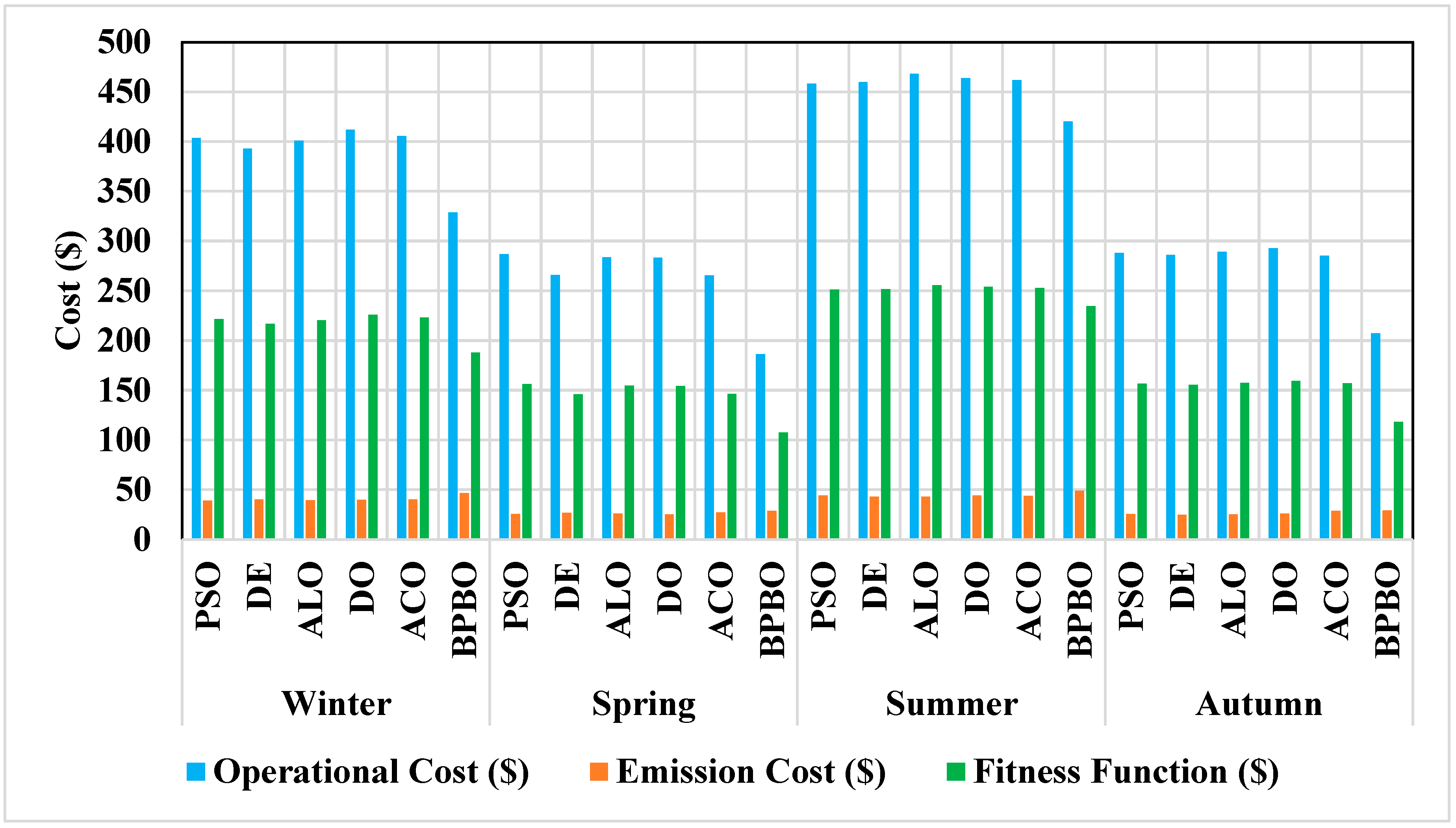
	BPBO	207	29.335	118.17

and Figure 14 provide a detailed decomposition of the best fitness values into their constituent operational cost and emission cost components across all seasons and optimizers. This decomposition offers critical insights into the multi-objective optimization trade-offs inherent in sustainable MG operation.

6.3.1. Seasonal Cost Patterns

Summer consistently exhibits the highest operational costs across all optimizers, ranging from 420.21 $ (BPBO) to 467.91 $ (ALO), reflecting the season’s extreme cooling, loads necessitating maximum utilization of expensive conventional generation. Winter operating costs occupy the second-highest tier at 328.64 $–411.65 $, driven by heating demands and reduced renewable availability. Spring and autumn demonstrate substantially lower dispatch costs (186.15 $–292.65 $), benefiting from moderate loads and abundant renewable resources. This seasonal cost stratification ranges from two to two and a half times between summer peaks and spring valleys, quantifying the profound economic impact of seasonal variability on MG economics.

Emission costs exhibit a more complex seasonal pattern. Winter shows moderate emissions (39.05 $–46.57 $), and summer displays elevated emissions (42.97 $–48.88 $), while spring and autumn achieve the lowest emission costs (24.98 $–29.34 $). The emission cost variation (approximately 1.8 times from minimum to maximum) proves less dramatic than operational cost variation, suggesting that renewable energy penetration, the primary emission reduction mechanism, exhibits moderate seasonal fluctuation, whereas load-driven operating costs demonstrate more extreme seasonality.

6.3.2. BPBO Performance Advantage

The proposed BPBO optimizer consistently achieves the lowest total fitness across all seasons, demonstrating robust superiority over competing algorithms. For winter, BPBO attains 187.60 $ compared to the next-best DE at 216.56 $, representing a 13.4% improvement. Spring season shows BPBO’s most dramatic advantage: 107.49 $ versus DE’s 146.17 $, a remarkable 26.5% cost reduction. Summer season yields 234.54 $ for BPBO against DE’s 251.51 $ (6.8% improvement), while autumn produces 118.17 $ versus DE’s 155.52 $ (24.0% improvement).

Interestingly, BPBO achieves these superior total fitness values despite occasionally exhibiting higher emission costs compared to other optimizers. For instance, in winter, BPBO’s emission cost of 46.57 $ exceeds PSO’s 39.05 $, yet the total fitness remains lowest due to substantially reduced economic costs (328.64 $ versus 403.62 $). This phenomenon reveals BPBO’s sophisticated optimization philosophy: it explores the Pareto frontier more comprehensively, identifying operating points where modest emission increases yield disproportionately larger operational cost savings. Given the equal 50% weighting of both objectives, BPBO’s strategy proves mathematically optimal, achieving lower total weighted costs than algorithms that narrowly focus on emission minimization at the expense of operational economics.

6.4. Statistical Performance Comparison

Table 6. Statistical analysis considering seasonal variation.

Season	Optimizer	Best	Mean	Worst	Std	Mean Time (s)
Winter	PSO	221.3342	237.0220	260.3787	10.2325752	0.5109
	DE	216.5586	226.0407	235.8830	4.60617417	0.5014
	ALO	220.1896	333,333,568	1 × 1010	1,825,741,814	3.7879
	DO	225.833	235.6856	258.1085	7.6752	0.7023
	ACO	222.9873	239.2809	254.1709	7.5199	0.6115
	BPBO	187.6012	200.7063	228.2522	9.3467	0.4908
Spring	PSO	156.1853	179.7851	214.5303	18.083	0.5412
	DE	146.1686	159.4530	173.0351	6.3093	0.5107
	ALO	154.7999	192.7634	264.6031	32.537	3.8866
	DO	154.1241	666,666,827	1 × 1010	2,537,081,274	0.7357
	ACO	146.4161	172.0218	195.3626	10.2978	0.6237
	BPBO	107.4937	123.3354	151.3503	8.8439	0.4885
Summer	PSO	251.1946	284.7121	317.9886	23.4577	0.5493
	DE	251.5053	263.2707	277.7926	6.9115	0.5578
	ALO	255.4366	333,333,618	1 × 1010	1,825,741,805	4.0451
	DO	254.0617	333,333,594	1 × 1010	1,825,741,809	0.7829
	ACO	252.7658	270.5533	286.6199	11.5266	0.7868
	BPBO	234.5438	244.3535	264.4906	7.0453	0.5409
Autumn	PSO	156.8178	184.1527	220.8776	18.0375	0.5341
	DE	155.5214	162.4446	170.2612	3.7926	0.5850
	ALO	157.2835	193.3976	244.9247	27.9447	4.2481
	DO	159.3585	177.4124	193.5640	9.1893	0.9328
	ACO	157.0228	179.5082	203.6643	13.1441	0.9436
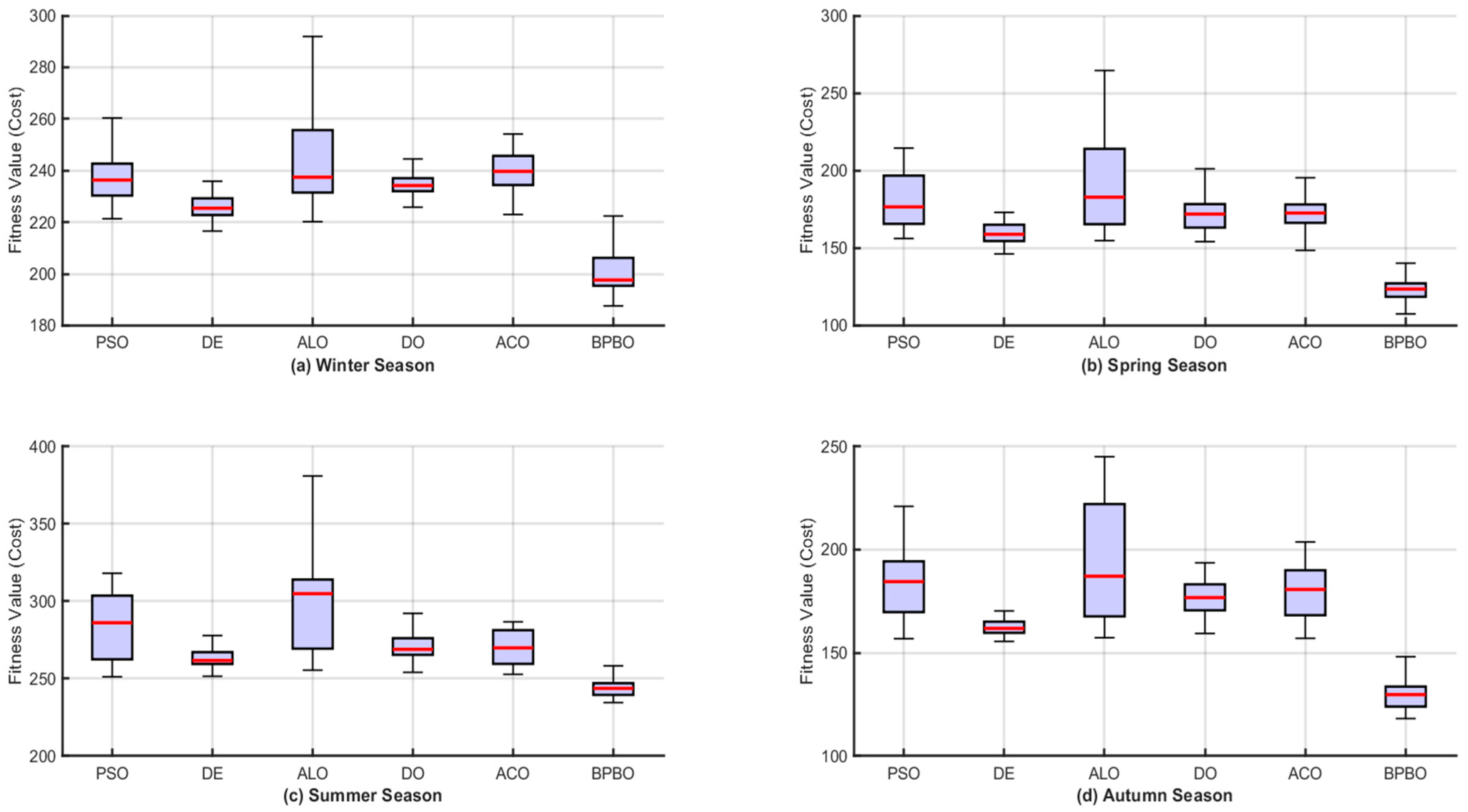
	BPBO	118.1673	129.9124	156.3883	8.1723	0.7086

presents comprehensive statistical metrics, best, mean, worst, standard deviation, and computational time, enabling rigorous multi-criteria assessment of algorithm performance across 30 independent runs per seasonal scenario. Figure 15 visualizes these distributions through box plots, clearly illustrating central tendencies, dispersion, and outlier characteristics.

6.4.1. Solution Quality Metrics

• Best Fitness: BPBO consistently delivers the lowest best fitness across all seasons: winter: 187.60 $, spring: 107.49 $, summer: 234.54 $, and autumn: 118.17 $. The second-ranked algorithm varies seasonally (DE in winter/spring and ALO in summer/autumn) but consistently underperforms BPBO by 13–27%. This unwavering best-case superiority establishes BPBO as the premier optimizer for MG energy management.
• Mean Fitness: Mean values reveal algorithm consistency across multiple runs. BPBO maintains excellent means—winter: 200.71 $, spring: 123.34 $, summer: 244.35 $, and autumn: 129.91 $—closely tracking the best fitness values. The small best-to-mean gaps (6–15%) indicate reliable convergence to near-optimal solutions in most runs. Competing algorithms exhibit substantially larger best-to-mean gaps: PSO shows 7–15% degradation, while DO suffers catastrophic failures with mean values exceeding 333 million (essentially infinite), indicating frequent convergence to infeasible solutions.
• Worst Fitness: BPBO’s worst-case performance remains competitive: winter: 228.25 $, spring: 151.35 $, summer: 264.49 $, and autumn: 156.39 $. These worst values still outperform or match the best values of inferior algorithms like DO and ALO in several scenarios. Conversely, ALO and DO demonstrate worst-case failures reaching 1 × 10¹⁰, representing constraint violations with maximum penalty application. Such catastrophic failures disqualify these algorithms for real-world deployment where reliability is paramount.
• Standard Deviation: BPBO maintains moderate standard deviations (winter: 9.35, spring: 8.84, summer: 7.05, and autumn: 8.17), indicating reasonable solution stability. DE achieves slightly lower standard deviations (4.61–6.91), suggesting tighter convergence but at higher mean fitness levels. PSO and ACO show larger variations (7.52–23.46), reflecting less consistent optimization performance. The extreme standard deviations of ALO (27.94–1.83 × 10⁹) and DO (7.68–2.54 × 10⁹) underscore their fundamental instability, rendering them unsuitable for practical MG applications.

6.4.2. Computational Efficiency

Computational time analysis reveals critical practical considerations. BPBO achieves remarkably fast execution: winter: 0.49 s, spring: 0.49 s, summer: 0.54 s, and autumn: 0.71 s. These times prove competitive with or faster than DE (0.50–0.59 s) and PSO (0.51–0.55 s), while being substantially faster than ACO (0.61–0.94 s) and DO (0.70–0.93 s). ALO suffers from excessive computational complexity (3.79–4.25 s), approximately 7–9 times slower than BPBO, likely due to the complex random walk mechanisms inherent in antlion-based search.

The computational efficiency of BPBO becomes particularly significant for real-time MG control applications where optimization must be completed within seconds to accommodate 5-to-15 min control intervals typical of energy management systems. Sub-second execution times enable BPBO deployment in computationally constrained embedded controllers or distributed control architectures, whereas multi-second algorithms like ALO may necessitate powerful centralized computing infrastructure.

The computational time reported in Table 6 represents the average runtime over 30 independent runs for each algorithm and seasonal case. The same population size, maximum number of iterations, scheduling horizon, and number of representative scenarios are used in all seasons. Therefore, the theoretical computational structure is the same for each seasonal case.

However, the measured runtime is not exactly identical because each season has different renewable-generation profiles, load-demand levels, electricity price patterns, and representative uncertainty scenarios. These differences affect the feasibility of candidate dispatch schedules and may require different numbers of constraint checks, boundary corrections, and SOC recalculations during the optimization process. In addition, small variations can occur due to random initialization and normal computer execution overhead. Therefore, the computation times are comparable across seasons but are not expected to be exactly the same.

6.5. Convergence Behavior Analysis

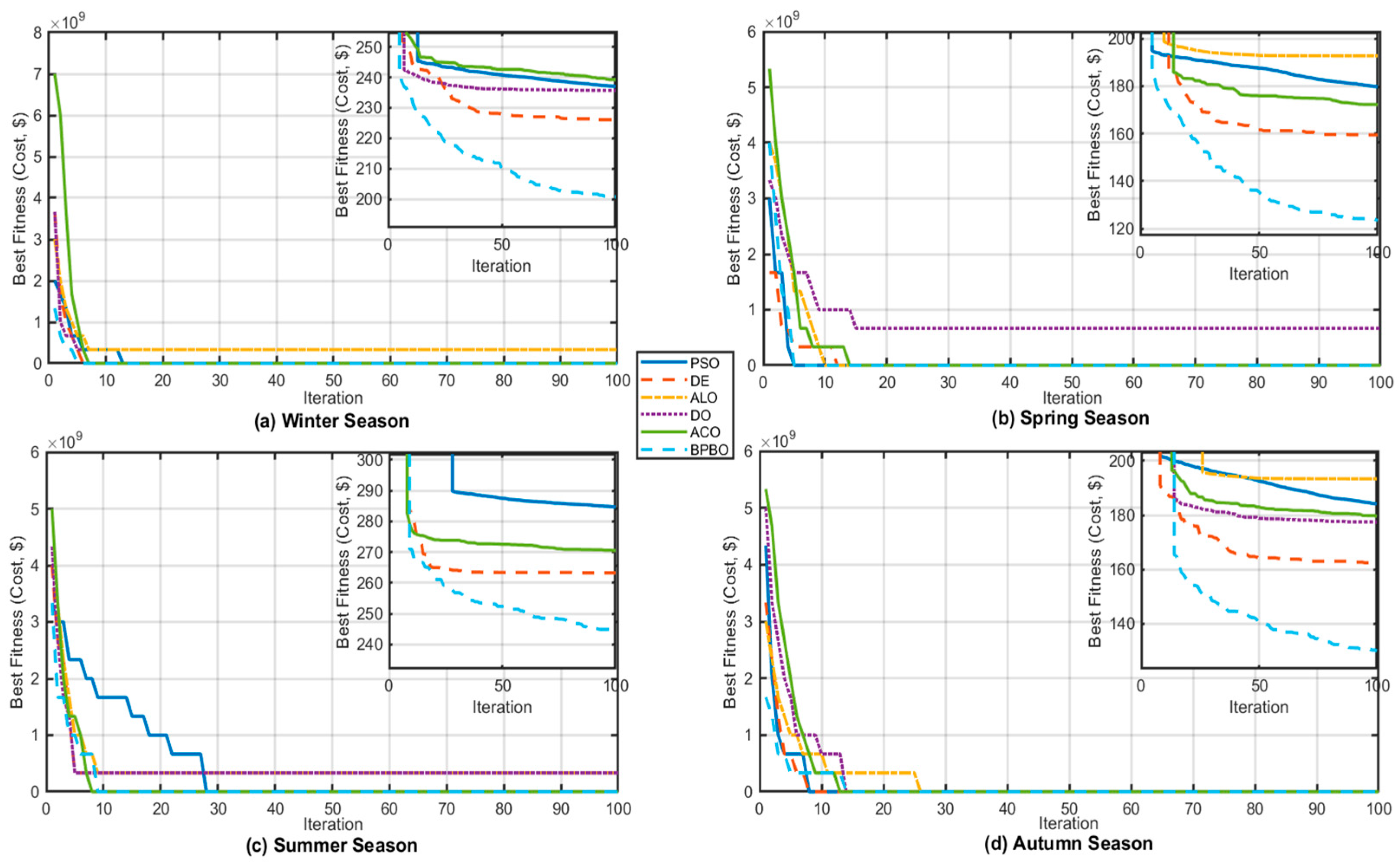
Figure 16 presents comprehensive convergence curves tracking the evolution of best fitness values across 100 optimization iterations for all six algorithms (PSO, DE, ALO, DO, ACO, and BPBO) under four seasonal operating scenarios. Each subplot includes both full-scale and zoomed-in inset views, enabling detailed examination of convergence dynamics in the critical final fitness range. These curves provide essential insights into search efficiency, exploitation-exploration balance, convergence rate, and algorithmic stability, critical performance dimensions for practical MG deployment.

6.5.1. Convergence Speed

Quantitative convergence rate comparison reveals BPBO’s consistent superiority across all seasons. Defining computational convergence as the iteration count required to reach within 5% of final fitness, BPBO achieves convergence in approximately 10–15 iterations across all seasons. DE requires 30–50 iterations, PSO and ACO need 25–40 iterations, while ALO often fails to converge even after 100 iterations, exhibiting continuous oscillations.

The rapid convergence characteristic proves particularly valuable for real-time MG control applications where optimization must be executed within seconds to accommodate 5-to-15 min dispatch intervals. If each iteration requires approximately 5 milliseconds of computation (based on Table 6 timing data with 100 iterations requiring 0.49–0.71 s for BPBO), then BPBO achieves near-optimal solutions in approximately 50–75 milliseconds, enabling potential deployment in high-frequency control scenarios or real-time pricing response applications.

6.5.2. Solution Quality Refinement Phase

A critical distinction between BPBO and competing algorithms emerges in the solution refinement phase (iterations 20–100). BPBO curves show continued gradual fitness reduction throughout this phase, with the zoomed-in insets revealing incremental improvements of 2 $–5 $ between iterations 20 and 100. This sustained refinement capability indicates BPBO maintains population diversity through stochastic Gaussian sampling, preventing complete convergence to a single point and enabling continued local search around the best-known solution.

In contrast, PSO and ACO exhibit flat convergence curves beyond iteration 30–40, indicating zero improvement in the refinement phase. This stagnation results from premature loss of population diversity when all particles/ants cluster around local optima, eliminating exploratory capability. DE maintains modest refinement capability, showing small but consistent improvements throughout iterations 30–100, attributable to its mutation-based diversity preservation mechanism.

The refinement phase improvements, while seemingly minor (2 $–5 $), translate into meaningful operational savings. For an MG operating 365 days annually, a 5 $ daily improvement yields 1825 $ annual savings, which is economically significant for small-scale distributed energy systems with tight economic margins.

6.5.3. Algorithmic Stability Assessment

Convergence curve smoothness provides critical insights into algorithmic stability. BPBO demonstrates exceptionally smooth, monotonically decreasing trajectories across all seasons, with no visible upward fitness jumps. This stability indicates robust search dynamics where each iteration reliably maintains or improves upon the best-known solution. DE and PSO show comparable stability with smooth curves exhibiting minimal fluctuations.

Conversely, ALO exhibits pronounced instability across all seasons, with convergence curves showing multiple sharp upward spikes where fitness temporarily increases by 10 $–50 $. These spikes occur because ALO’s random walk mechanism can generate solutions inferior to the current best, temporarily degrading the population’s best-known solution until superior alternatives are discovered. While such exploration behavior theoretically benefits global search, the frequency and magnitude of these instabilities in the MG application suggest poor algorithm-problem compatibility.

DO’s stability varies dramatically by season and runs, ranging from smooth convergence in successful runs to complete divergence in failed runs (visible in the astronomical mean fitness values in Table 6). This unpredictable behavior stems from DO’s dandelion seed dispersion mechanism, which can cause the population to explore excessively distant regions of the solution space, frequently violating constraints in high-dimensional problems like 192-variable MG optimization.

6.5.4. Seasonal Convergence Difficulty Assessment

Comparing convergence patterns across seasons reveals relative problem difficulty. Spring and autumn exhibit the fastest multi-algorithm convergence with the lowest final fitness values, suggesting that these seasons present well-structured optimization landscapes with clear gradients toward optimal solutions. The abundant renewable resources and moderate loads create favorable conditions where multiple dispatch strategies achieve near-optimal performance.

Summer demonstrates the most challenging convergence characteristics, slower convergence rates, higher final fitness values, and multiple algorithm failures (ALO and DO). The extreme loads combined with reduced wind availability create a highly constrained solution space where feasible solutions occupy a small fraction of the total search space, requiring more sophisticated search strategies to avoid constraint violations.

Winter presents moderate difficulty, with convergence speeds and final fitness values falling between summer and spring/autumn. The seasonal convergence difficulty patterns provide valuable insights for algorithm selection and parameter tuning strategies. More robust algorithms with strong constraint handling prove essential for summer operation, while simpler methods may suffice for spring/autumn scenarios.

6.6. Discussion of Seasonal Performance Differences and Algorithmic Advantages

The comparative results indicate that the performance of the optimization algorithms is affected not only by their search mechanisms but also by the seasonal operating conditions of the MG. Each season creates a different scheduling environment because solar irradiance, wind speed, ambient temperature, electrical demand, and electricity price vary simultaneously. These variations change the size and shape of the feasible search space and directly influence the contribution of renewable generation, dispatchable units, ES, and grid exchange.

In spring and autumn, the MG operates under more favorable conditions because renewable generation is relatively available and the electrical demand remains moderate. These seasons provide greater scheduling flexibility, allowing the optimizer to select among several feasible combinations of renewable utilization, ES operation, dispatchable generation, and grid transactions. This explains the lower fitness values obtained in these seasons. The availability of wind and solar resources also reduces the need for continuous grid imports and allows the ES system to support the load more effectively during selected periods.

Summer represents the most constrained operating condition. Although PV generation is higher during this season, the increase in cooling-related demand creates a heavier load burden on the MG. At the same time, the lower wind contribution reduces the diversity of the renewable supply. Consequently, the optimizer must rely more frequently on the MT, FC, grid purchase, and battery discharge while still satisfying power-balance, generation-limit, grid-exchange, and state-of-charge constraints. Under these conditions, the feasible region becomes narrower, and the relative improvement among algorithms becomes smaller. This explains why the performance advantage of BPBO in summer is lower than that observed in spring and autumn.

Winter also presents a challenging scheduling condition, but for different reasons. The reduction in solar irradiance limits PV contribution, especially during early and late hours, while demand remains relatively high during morning and evening periods. This increases the dependence on dispatchable generation and grid purchase. However, compared with summer, the load level is less extreme, which gives the optimizer slightly more flexibility in coordinating the ES system and conventional generation units. Therefore, the winter results fall between the highly constrained summer case and the more flexible spring and autumn cases.

The superior performance of BPBO can be attributed to its balanced exploration and exploitation behavior. In the early search stage, BPBO explores a wide range of candidate schedules, which helps identify promising operating regions and reduces the probability of premature convergence. In later iterations, the algorithm refines the best candidate solutions and improves the coordination among the available energy resources. This behavior is particularly important in the studied scheduling problem because the decision variables are temporally coupled through the ES state of charge. A charging or discharging decision at one hour affects the feasible operating range in subsequent hours, making the problem more complex than a set of independent hourly dispatch decisions.

Compared with the other tested metaheuristic algorithms, BPBO shows a stronger ability to maintain solution quality across different seasonal conditions. Algorithms with rapid but less diverse search behavior may converge early to local solutions, especially when renewable generation and demand profiles create tight operational constraints. On the other hand, algorithms with excessive random exploration may produce infeasible or heavily penalized schedules. BPBO provides a more suitable compromise between these two behaviors, allowing it to reduce the total fitness value while maintaining acceptable convergence stability and computational time.

The results also show that BPBO is able to manage the economic–environmental trade-off more effectively than the competing algorithms. The objective function considers both operating costs and emission costs; therefore, the best solution is not necessarily the one with the lowest emission component alone or the lowest operating component alone. Instead, the optimizer must find a balanced dispatch schedule that minimizes the weighted objective. BPBO achieves lower total fitness values by coordinating renewable generation, dispatchable units, ES operation, and grid exchange in a way that improves the overall objective value. This explains why the proposed method can outperform other algorithms even when some individual cost components are not always the lowest.

From an operational perspective, the main advantage of BPBO is its ability to adapt the dispatch schedule to the available seasonal flexibility. In spring and autumn, the algorithm benefits from higher renewable availability and moderate demand by increasing the contribution of renewable generation and using the ES system more strategically. In summer, when the load is high and the system operates closer to its technical limits, BPBO still maintains the lowest fitness value by coordinating all available resources under tighter constraints. In winter, it compensates for reduced solar generation by balancing dispatchable generation, storage operation, and grid purchase.

6.7. Generalizability and Scalability of the Proposed BPBO-Based Scheduling Framework

Although the numerical results reported in this study are based on a representative grid-connected multi-energy MG with specific component ratings and seasonal operating profiles, the proposed BPBO-based scheduling framework is not limited to this particular configuration. The algorithm operates on a decision vector defined by the dispatch variables, system constraints, and lower and upper bounds of the controllable resources. Therefore, the same framework can be applied to other MG sizes and regions by updating the PV and wind capacities, dispatchable-unit ratings, energy storage capacity, grid-exchange limits, load demand, electricity-tariff structure, and renewable-resource profiles. Different climatic conditions can also be represented by modifying the hourly mean values and probability-distribution parameters of solar irradiance, wind speed, ambient temperature, load demand, and electricity price. Accordingly, BPBO is expected to remain applicable under different climates, tariffs, and component ratings; however, the resulting dispatch schedules, cost savings, emission reductions, and convergence behavior may vary depending on the local resource availability, demand characteristics, tariff design, and system constraints. Future work will therefore extend the validation to larger MG configurations, different geographical regions, measured site-specific data, and alternative tariff structures to further assess the scalability and transferability of the proposed approach.

From a computational perspective, the scalability of the proposed method mainly depends on the number of decision variables, representative scenarios, optimization iterations, and operational constraints. Larger MGs with additional buses, dispatchable generators, renewable units, storage systems, or controllable loads will increase the dimension of the decision vector and the number of constraint evaluations. Similarly, longer scheduling horizons will increase the number of hourly dispatch variables and storage-state updates. In general, the computational effort of the BPBO-based scheduling process can be related to the population size, maximum number of iterations, number of representative scenarios, scheduling horizon, and number of controllable resources. Nevertheless, the use of FFS reduces the stochastic scenario set before optimization, which helps limit the computational burden. For larger-scale applications, parallel fitness evaluation, adaptive population sizing, decomposition strategies, or rolling-horizon implementation can be used to improve computational efficiency. Therefore, while the runtime results obtained in this study are promising for the investigated test system, further assessment on larger multi-bus MGs and extended scheduling horizons is recommended.

6.8. Battery Degradation and Lifecycle Cost Discussion

The ES system plays an important role in the proposed scheduling framework because it supports renewable-energy utilization, reduces grid purchases during peak-price periods, and improves MG flexibility. In the present formulation, the storage model includes charging and discharging efficiencies, power limits, state-of-charge bounds, and a cyclic final state-of-charge constraint. These constraints maintain feasible storage operation and prevent unrealistic deep depletion or overcharging. However, the model does not explicitly include battery degradation or lifecycle cost.

This assumption should be considered when interpreting the economic results. Frequent charge–discharge cycling can accelerate battery aging, reduce usable capacity, and increase replacement cost over the project lifetime. Therefore, excluding degradation cost may overestimate the net economic benefit of storage, especially in seasons where the battery is used intensively to support peak demand or compensate for renewable-generation fluctuations. A more detailed degradation-aware formulation can be introduced by adding a cycling cost term to the objective function. For example, the degradation cost may be estimated as a function of battery replacement cost, rated energy capacity, depth of discharge, charge/discharge throughput, and equivalent cycle life. This additional term would discourage excessive cycling when the economic savings from storage operations are lower than the associated aging cost.

Accordingly, battery degradation modeling is identified as an important extension of the present work. Future research will incorporate degradation-aware storage scheduling to evaluate the trade-off between short-term operating-cost reduction and long-term battery lifecycle cost. This extension will provide a more comprehensive assessment of the economic feasibility of storage-intensive MG operation.

6.9. Limitations

Despite the advantages, some limitations should be acknowledged. First, the seasonal profiles used in this study are representative simulation profiles rather than measured data from a specific MG site. Therefore, the numerical results should be interpreted as a controlled case-study assessment of the proposed scheduling framework rather than a site-specific operational validation. Future work should test the method using measured meteorological, load, and electricity price data from real MG installations.

Second, the study considers a fixed MG configuration and a 24 h day-ahead scheduling horizon. Larger systems with additional buses, renewable units, storage devices, controllable loads, and network constraints may increase the number of decision variables and the complexity of the optimization problem. Although the computation times obtained in this study are promising, further investigation is required to evaluate the scalability of BPBO for larger and more detailed MG models.

Third, the current formulation constrains the ES system through charging and discharging limits, SOC limits, and a cyclic final SOC condition. These constraints help avoid unrealistic storage operations, but they do not explicitly account for battery degradation cost or lifetime reduction caused by frequent cycling. Including a degradation-aware storage cost model would provide a more complete economic assessment, especially in cases where the battery is used intensively to reduce grid imports or support peak demand.

Finally, the comparison in this study includes several well-known metaheuristic algorithms, which provide a useful benchmark for evaluating BPBO. However, additional comparisons with other recent optimizers, hybrid methods, mathematical programming approaches, and learning-assisted scheduling techniques would further strengthen the assessment. Future studies may also combine BPBO with forecasting models or artificial intelligence techniques to improve uncertainty representation for renewable generation, load demand, and electricity prices.

Overall, the expanded discussion shows that the performance differences among the algorithms are closely related to both algorithmic behavior and seasonal operating conditions. BPBO provides the best overall performance in the studied cases because it maintains an effective balance between search diversification, solution refinement, constraint handling, and computational efficiency. At the same time, further validation using measured data, larger test systems, battery degradation modeling, and broader algorithmic comparisons is recommended to confirm its applicability under more practical operating conditions.

7. Conclusions

This study proposed a stochastic day-ahead scheduling framework for a grid-connected multi-energy MG under seasonal renewable uncertainty. The proposed framework combined probabilistic uncertainty modeling, MC scenario generation, FFS scenario reduction, and BPBO. The studied MG included PV generation, wind generation, an MT, an FC, an ES system, and utility-grid exchange. The scheduling objective minimized a weighted combination of operating cost and emission cost while satisfying generation, storage, power-balance, and grid-exchange constraints.

The results showed that BPBO achieved the best fitness value among the compared metaheuristic algorithms in all four seasonal cases. The proposed method reduced the total fitness value by 15.2% in winter, 26.5% in spring, 6.8% in summer, and 23.9% in autumn compared with the second-best optimizer. The seasonal analysis also showed that summer produced the highest operating cost and emission cost because of increased cooling demand and lower wind contribution, while spring and autumn provided more favorable operating conditions due to better renewable availability and moderate load demand.

The findings confirm that the proposed BPBO-based scheduling framework can effectively coordinate dispatchable generation, renewable generation, ES operation, and grid exchange under stochastic seasonal conditions. The use of FFS reduced the original MC scenario set from 1000 scenarios to 10 representative scenarios, which improved computational practicality while preserving the main uncertainty characteristics required for scheduling.

Future work will extend the proposed framework to larger multi-bus MG systems, measured site-specific datasets, alternative tariff structures, and longer scheduling horizons. Battery degradation cost and artificial-intelligence-based uncertainty forecasting will also be considered to improve the practical applicability and long-term economic assessment of storage-intensive MG operation.