Cooperative Learning NN-Based Fault-Tolerant Formation of Networked Unmanned Surface Vehicles with Input Saturation and Prescribed Performance

Abstract

This paper investigates the cooperative formation control problem in unmanned surface vehicles (USVs) with prescribed performance constraints under complex marine conditions including external disturbances, model uncertainties, actuator faults, and input saturation. A novel fault-tolerant control (FTC) algorithm is developed by integrating cooperative learning neural networks (NNs), distributed disturbance observers, and the backstepping technique. Specifically, the learning NNs adaptively approximate system uncertainties, and the learned weight information is shared among vehicles to enhance cooperative cognition. Additionally, an auxiliary dynamic system and an actuator configuration matrix are designed to compensate for input saturation and propeller failures. Theoretical analysis based on the Lyapunov method proves that all signals in the closed-loop system are bounded, and the formation tracking errors strictly remain within the predefined transient and steady-state performance bounds. Finally, simulation experiments involving a group of four USVs validate the proposed algorithm. The results demonstrate that the USVs can rapidly converge to and maintain the desired quadrilateral formation shape despite time-varying disturbances and actuator efficiency loss. Furthermore, comparative simulation results indicate that the proposed cooperative learning FTC scheme significantly reduces velocity tracking error oscillations compared to traditional non-learning methods, explicitly verifying its superior robustness and fault-tolerant capabilities.

1. Introduction

As is well known, marine resource exploration has always been a hot topic in the field of ocean engineering. With the increasing attention on the field, surface vehicles are required to possess various tools for exploring and developing marine resources, particularly in harsh ocean environments. Unmanned surface vehicles (USVs) have gained significance due to their feasibility, flexibility, and low mission cost [1,2,3,4], playing a crucial role in marine engineering [5]. However, in the face of more complex ocean environments, a single USV is no longer sufficient to meet the demands of exploration and resource development [6]. Subsequently, multiple USVs, offering advantages of enhanced robustness, adaptability, and reliability, have been developed [7,8,9], and vehicles have achieved behaviors, such as formation, containment, and flocking by designing proper cooperative algorithms [10].

In the design of formation control, various methods have been proposed including finite-time control [11], integral sliding-mode control [12], and backstepping control [13]. Note that the backstepping control method is designed in a straightforward manner and can achieve system stability through a step-by-step recursive process. It is particularly advantageous in handling strong couplings for nonlinear systems with various disturbances, and it is widely applied for the formation control of systems. For instance, Jiang et al. [14] designed an efficient state observer-based backstepping method to record the system states. In practical applications, the redundancy in the actuator interactions within the overactuated system always leads to the occurrence of actuator failures. For example, stuck (or hardover) failures affecting multiple actuators often trigger saturation phenomena in the remaining functional actuators, ultimately giving rise to system instability [15] and significantly increasing the possibility of actuator failure. Therefore, it is necessary to use a variable actuator configuration matrix, allocate signal computations to individual actuators, and minimize the overall system power consumption [16]. In the process of control allocation, it is essential to take into account adverse effects of actuator failures caused by factors such as operating duration or external environmental influences on control systems [17]. Hence, it is crucial to develop fault-tolerant control (FTC) algorithms to ensure safety and dependability of vehicle systems. Liang et al. [18] proposed an underactuated adaptive FTC algorithm that estimated and compensated for the impact of actuator faults by using an observer. Liu et al. [19] proposed a fixed-time FTC algorithm for USVs with external disturbances, that combined the estimator with a fixed-time sliding-mode surface to solve unknown effects caused by actuator failures. In practical applications, uncertainties in dynamics are inevitable; as such, system uncertainties represent a problem that must be considered in the design of control systems.

Commonly used methods to solve uncertainties include fuzzy adaptive control and neural network (NN) control [20]. NNs have incredibly powerful capabilities for easily handling some common problems. Typically, they are used to approximate the uncertainties in systems [21] and achieve adaptive estimation of unknown terms by updating the weights of the NNs [22]. Skjetne et al. [23] estimated the unknown terms of the system using NNs and designed an adaptive auxiliary system to achieve finite-time convergence by minimizing parameters. Tsolakis et al. [24] proposed an NN-based observer to estimate the unknown terms, which achieved state constrained tracking control of surface vehicles. The above results mainly focus on achieving stability of the control systems but neglect the strong learning ability of NNs, namely, only self-updating of NN weights is used in traditional NN adaptive control [25]. Moreover, in most NN-based control methods, the weights of the NNs have difficulty in converging to the optimal values [26]. In addition to the previously mentioned issues such as actuator faults and unknown parameters, one aspect that needs to be considered is external disturbances such as waves, hurricanes, and other marine environmental factors that may change over time. These conditions can affect the accuracy of NN estimation, and in more severe cases, they can lead to the failure of the vehicles’ state convergence.

In addition, there are always special requirements for control inputs and outputs in the process of control systems. The input of the system is limited and cannot reach the theoretically unrestricted range, so input saturation is a common problem encountered in the system. Wang et al. [27] proposed a finite-time controller that introduced a saturation function to solve the input saturation issue. Wang et al. [28] utilized a strategy of combining NNs with dynamic surfaces and introduced an auxiliary system to compensate for input saturation effects. Additionally, the outputs of practical equipment are also subject to specific constraints. For example, the movement of vehicles must be within certain ranges and the stroke of the hydraulic cylinder needs to be limited during specific tasks. Therefore, research on output constraints of systems has become increasingly important. Yan et al. [29] studied the tracking control of vehicles formations with prescribed performance, and then proposed control strategies to ensure that leaders and followers maintained contact within prescribed performance limits without conflicts [30]. The constrained control problems have always been a hot research topic, but how to settle the complex issue of faulted USVs with simultaneous input and output constraints is still challenging.

Based on the above analysis and discussion, this paper mainly focuses on the complex formation tracking of uncertain USVs subject to propeller failures, input and output constraints. A learning NN-based FTC algorithm is designed by combining NNs with backstepping. The innovation can be summarized in three key aspects.

I1:

Compared to previous results that neglect the constraints of inputs and outputs, an FTC algorithm is designed to maintain the prescribed performance of systems such that it can achieve adaptive formation tracking of USVs even with actuator failures or redundancy.

I2:

The proposed control algorithm settles the model uncertainties by estimating unknown dynamics with learning NNs. It stores and employs the learned update knowledge of NN weights from other vehicles, and hence it can easily achieve optimal performance of formation tracking through more robust mechanism of information sharing.

I3:

An adaptive auxiliary variable is introduced in the algorithm to effectively address the input saturation issue, ensuring that the system operates within prescribed performance bounds. Meanwhile, the influence of time-varying disturbances on the estimation information is reduced by designing a disturbance observer. Therefore, the control system states tend to stabilization and consistently maintain the prescribed performance.

The remaining sections are organized as follows: Section 2 provides an introduction to the foundational knowledge and problem description. Section 3 presents the main results, including the design of the cooperative learning NN-based FTC algorithm, which demonstrates the system ability to maintain prescribed performance and proves the algorithm convergence. Section 4 and Section 5 present the simulation studies and the final conclusion, highlighting the effectiveness of the control algorithm.

Notations: R, ${\mathbb{R}}^p$ and ${\mathbb{R}}^{p\times p}$ are all real matrices. ⊗ denotes the Kronecker product. $∥·∥$ is the Euclidean norm. $I_{n\times n}$ is an $n\times n$ identity matrix. $\mathrm{diag}\{·\}$ is a diagonal matrix. ${\lambda }_{min}(·)$ and ${\lambda }_{max}(·)$ are the minimum and maximum eigenvalues, respectively.

2. Preliminaries and Formulation

2.1. Graph Theory

An undirected graph $\mathcal{G}=\left\{\mathcal{N},\mathcal{E},\mathcal{A},\mathcal{L}\right\}$ is used to describe the interactions among USVs, with $\mathcal{N}=\{1,\dots ,n\}$ as the vertex set indexed by each vehicle, $\mathcal{E}\subseteq \mathcal{N}\times \mathcal{N}$ as the edge set, $\mathcal{A}={\left[a_{ij}\right]}_{n\times n}$ and $\mathcal{L}={\left[l_{ij}\right]}_{n\times n}$ as adjacency and Laplacian matrices. An edge $\left\{i,j\right\}\in \mathcal{E}$ with $a_{ij}=1$ if the i-th and j-th vehicles can transfer information, and $a_{ij}=0$, otherwise. Additionally, $l_{ij}={\sum }_{j=1}^n{a}_{ij}$ for $i=j$, and $l_{ij}=-a_{ij}$ for $i\ne j$.

2.2. Problem Formulation

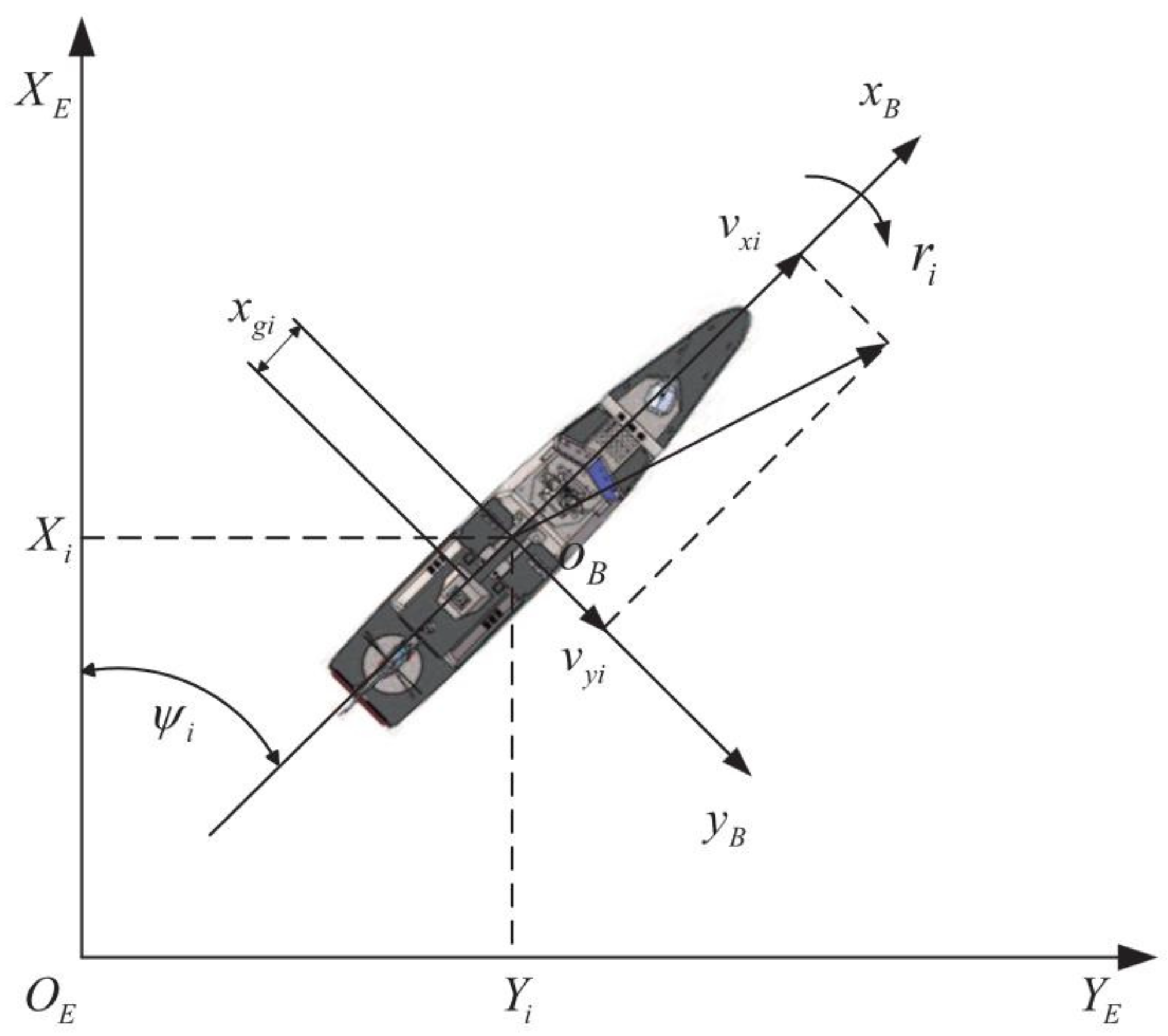
With the earth-fixed and body-fixed frames shown in Figure 1, the kinematics and dynamics of USVs are described by the following equation:

$$\begin{array}{c}{\dot{\eta }}_i=R\left({\psi }_i\right)v_i,\hfill \\ M{\dot{v}}_i+C\left(v_i\right)v_i+D\left(v_i\right)v_i+\rho ({\eta }_i,v_i)={\tau }_{f,i}+d_i,\hfill \end{array}$$

(1)

where ${\eta }_i={\left[x_i,y_i,{\psi }_i\right]}^T\in {\mathbb{R}}^3$ represents the position vector $(x_i,y_i)$ and yaw angle ${\psi }_i$ of vehicles in the earth-fixed coordinate frame, and ${\nu }_i={\left[u_i,v_i,r_i\right]}^T\in {\mathbb{R}}^3$ represents the linear velocity $(u_i,v_i)$ and yaw velocity $r_i$ in the body-fixed coordinate frame. $M=M^T\in {\mathbb{R}}^{3\times 3}$ is the symmetric positive definite inertia matrix, and $C\left({\nu }_i\right)\in {\mathbb{R}}^{3\times 3}$ denotes the total Coriolis and centripetal matrix. $D\left({\nu }_i\right)\in {\mathbb{R}}^{3\times 3}$ is the damping matrix, and $\rho ({\eta }_i,{\nu }_i)={[{\rho }_1,{\rho }_2,{\rho }_3]}^T\in {\mathbb{R}}^3$ indicates the unaccounted system dynamics stemming from unspecified parameter fluctuations. ${\tau }_{f,i}\in {\mathbb{R}}^3$ represents the faulted control input vector, and $d_i\in {\mathbb{R}}^3$ denotes the unknown time-varying disturbance. $R\left({\psi }_i\right)$ denotes the rotation matrix as

$$R\left({\psi }_i\right)=\left[\begin{array}{ccc}cos\left({\psi }_i\right)& -sin\left({\psi }_i\right)& 0\\ sin\left({\psi }_i\right)& cos\left({\psi }_i\right)& 0\\ 0& 0& 1\end{array}\right].$$

Note that the actuators of the vehicles are the same rotating propellers producing propulsive forces. Assume there are p propellers, and the k-th propeller is located at the position:

$$l_{k,i}=\left[l_{kx,i},l_{ky,i}\right],$$

where $l_{kx,i}$ and $l_{ky,i}$, $i\in \mathcal{N}$ represent the distance from propeller k to the origin of body-fixed coordinate, and a force $F_{k,i}$ can be generated in a direction determined by an orientation vector angle ${\varphi }_k$. Thus, the force generated by the k-th propeller has the following effects:

$$\begin{array}{c}{F}_{kx,i}=F_{k,i}cos\left({\varphi }_k\right),\hfill \\ F_{ky,i}=F_{k,i}sin\left({\varphi }_k\right),\hfill \\ T_{k,i}=F_{k,i}{N}_{k,i},\hfill \end{array}$$

where $N_{k,i}=l_{kx,i}sin\left({\varphi }_k\right)-l_{ky,i}cos\left({\varphi }_k\right)$, and the combination of the forces produced by all propellers are

$${\tau }_{f,i}=B\left(\varphi \right){\tau }_{s,i},$$

(2)

where ${\tau }_{s,i}={[{\tau }_{s,1},\dots ,{\tau }_{s,n}]}^T\in {\mathbb{R}}^{p\times 1}$ is the designed control input of the actuator, $B\left(\varphi \right)\in {\mathbb{R}}^{3\times p}$, $\varphi =[{\varphi }_1,\dots {\varphi }_p]\in {\mathbb{R}}^p$, is the configuration matrix with the form as follows:

$$B\left(\varphi \right)=\left[\begin{array}{cccc}cos\left({\varphi }_1\right)& cos\left({\varphi }_2\right)& \dots & cos\left({\varphi }_p\right)\\ sin\left({\varphi }_1\right)& sin\left({\varphi }_2\right)& \dots & sin\left({\varphi }_p\right)\\ N_1& N_2& \dots & N_p\end{array}\right].$$

(3)

In practice, the input is usually limited in a boundary as

$$-{\underline{\tau }}_{s,i}\le {\tau }_{s,i}\le {\overline{\tau }}_{s,i},$$

where ${\underline{\tau }}_{s,i}={[{\tau }_{s,1 min},\dots ,{\tau }_{s,n min}]}^T\in {\mathbb{R}}^{p\times 1}$ and ${\overline{\tau }}_{s,i}={[{\tau }_{s,1 max},\dots ,{\tau }_{s,n max}]}^T\in {\mathbb{R}}^{p\times 1}$ represent the lower and upper boundary of the input constraints, and ${\tau }_{s,i}$ is described as

$${\tau }_{s,i}=\left\{\begin{array}{cc}{\tau }_{s,i max},\hfill & \mathrm{if}{\tau }_{s,i}>{\tau }_{s,i max},\hfill \\ {\tau }_{s,i},\hfill & \mathrm{if}-{\tau }_{s,i min}\le {\tau }_{s,i}\le {\tau }_{s,i max},\hfill \\ -{\tau }_{s,i min},\hfill & \mathrm{if}{\tau }_{s,i}<-{\tau }_{s,i min},\hfill \end{array}\right.$$

(4)

The purpose of this paper is to force all vehicles to track the position ${\eta }_d$ of the reference trajectory while maintaining the prescribed shape. During this process, formation tracking error $e_i\in {\mathbb{R}}^3$ is generated, where ${∆}_i\in {\mathbb{R}}^3$ represents the formation offset, and $e_i$ is written as

$$e_i={\eta }_i-{\eta }_d-{∆}_i.$$

(5)

To ensure better control performance, the tracking error $e_i$ must remain within the boundaries of the following predetermined thresholds.

$$-{\underline{e}}_i\left(t\right)<e_i\left(t\right)<{\overline{e}}_i\left(t\right),$$

(6)

with the lower bound ${\underline{e}}_i$ and upper bound ${\overline{e}}_i$ as

$$\begin{array}{c}{\underline{e}}_i\left(t\right)=({\underline{e}}_{i,0}-{\underline{e}}_{i,\infty })exp(-{\mu }_{i}t)+{\underline{e}}_{i,\infty },\hfill \\ {\overline{e}}_i\left(t\right)=({\overline{e}}_{i,0}-{\overline{e}}_{i,\infty })exp(-{\mu }_{i}t)+{\overline{e}}_{i,\infty },\hfill \end{array}$$

(7)

where $e_{i,0}$, $e_{i,\infty }$ and ${\mu }_i$ are all parameters that need to be designed as positive with $e_{i,0}>e_{i,\infty }$, so as to constrain the accuracy of trajectory tracking. The objectives of this paper include the following two aspects:

Objective 1. 

USVs are able to achieve the expected formation while tracking the reference trajectory ${\eta }_d$.

$$\left\{\begin{array}{c}\underset{t\to \infty }{lim}∥{\eta }_i-{\eta }_d-{∆}_i∥=0,\hfill \\ \underset{t\to \infty }{lim}∥{\dot{\eta }}_i-{\dot{\eta }}_d∥=0,\hfill \end{array}\right.$$

Objective 2. 

To ensure the prescribed performance of the system, the formation tracking error $e_i$ always remains within the pre-designed upper and lower bounds.

$$-{\underline{e}}_i\left(t\right)<e_i\left(t\right)<{\overline{e}}_i\left(t\right).$$

For the sake of better development, we present some necessary assumptions and lemmas as follows.

Assumption A1. 

The undirected graph $\mathcal{G}$ is connected.

Assumption A2. 

The initial value of formation tracking error should satisfy $-{\underline{e}}_i\left(0\right)<e_i\left(0\right)<{\overline{e}}_i\left(0\right)$, $i\in \mathcal{N}$.

Assumption A3. 

The disturbances $d_i$ and first-order derivatives ${\dot{d}}_i$ are bounded with unknown upper boundary.

Assumption A4. 

The states of the reference trajectory ${\eta }_d$, ${\dot{\eta }}_d$, and ${\ddot{\eta }}_d$ are smooth, bounded and periodic signals.

Assumption A5. 

If $B\left({\varphi }_0\right)$ is a full row rank matrix with $rank\left(B\left({\varphi }_0\right)\right)=3<p$, a bounded uncertain actuator configuration matrix $∆B(∆\varphi )$ satisfies the following condition with a positive constant β.

$$∥∆B(∆\varphi )K∥<\beta {\hslash }_1.$$

Lemma 1 

([31]). If there exists a continuously positive definite Lyapunov function $V\left(x\right)$ that satisfies $\dot{V}\left(x\right)\le -\zeta V\left(x\right)+\delta$ with bounded $V\left(0\right)$, ζ and δ as positive constants, it can be deduced that $x\left(t\right)$ is uniformly bounded.

Lemma 2. 

For any $\alpha \in \mathbb{R}$, $\beta \in \mathbb{R}$, the following equation transformations can be applied:

$$sin(\alpha +\beta )=sin\alpha +\beta {\int }_0^{1}cos(\alpha +s\beta )ds=sin\alpha +\beta {\theta }_c(\alpha ,\beta ),$$

(8)

$$cos(\alpha +\beta )=cos\alpha -\beta {\int }_0^{1}sin(\alpha +s\beta )ds=cos\alpha -\beta {\theta }_s(\alpha ,\beta ),$$

(9)

with $|{\theta }_c(\alpha ,\beta )|\le 1$ and $|{\theta }_s(\alpha ,\beta )|\le 1$.

Proof. 

Assume that f is a continuously differentiable function defined on an open interval I. $\alpha$ and $\alpha +\beta$ are points in the open interval I. Then, one obtains [32]:

$$f(\alpha +\beta )-f\left(\alpha \right)={\int }_{\alpha }^{\alpha +\beta }{f}^{\prime }\left(\zeta \right)d\zeta .$$

(10)

Defining $\zeta =\alpha +s\beta$ and substituting it into (10), one obtains

$$f(\alpha +\beta )-f\left(\alpha \right)=\beta {\int }_0^1{f}^{\prime }(\alpha +s\beta )ds.$$

Let $f\left(\zeta \right)=sin\left(\zeta \right)$ or $f\left(\zeta \right)=cos\left(\zeta \right)$, and we can derive (8) and (9), separately. Furthermore, since the trigonometric functions satisfy $sin\left(\zeta \right)\le 1$ and $cos\left(\zeta \right)\le 1$, we can obtain $|{\theta }_s(\alpha +\beta )|=|{\int }_0^{1}sin(\alpha +s\beta )ds|\le {\int }_0^1|sin(\alpha +s\beta \left)\right|ds\le 1$ and $|{\theta }_c(\alpha +\beta )|=|{\int }_0^{1}cos(\alpha +s\beta )ds|\le 1$. □

Lemma 3 

([33]). For all continuous cyclic trajectories $X\left(t\right)\in [0,\infty )\to {\mathbb{R}}^q$, $X\left(t\right)$ remains within a compact set ${\mathrm{\Omega }}_x$ with ${\mathrm{\Omega }}_x\subset {\mathbb{R}}^q$. The center of the NN $W^{T}h\left(x\right)$ is maintained on a regular lattice. It is large enough to cover the compact set ${\mathrm{\Omega }}_x$, and the regress subvector $h_{\zeta }\left(x\right)$ maintains a continuous excitation.

3. Learning NN Formation with Input and Output Constraints

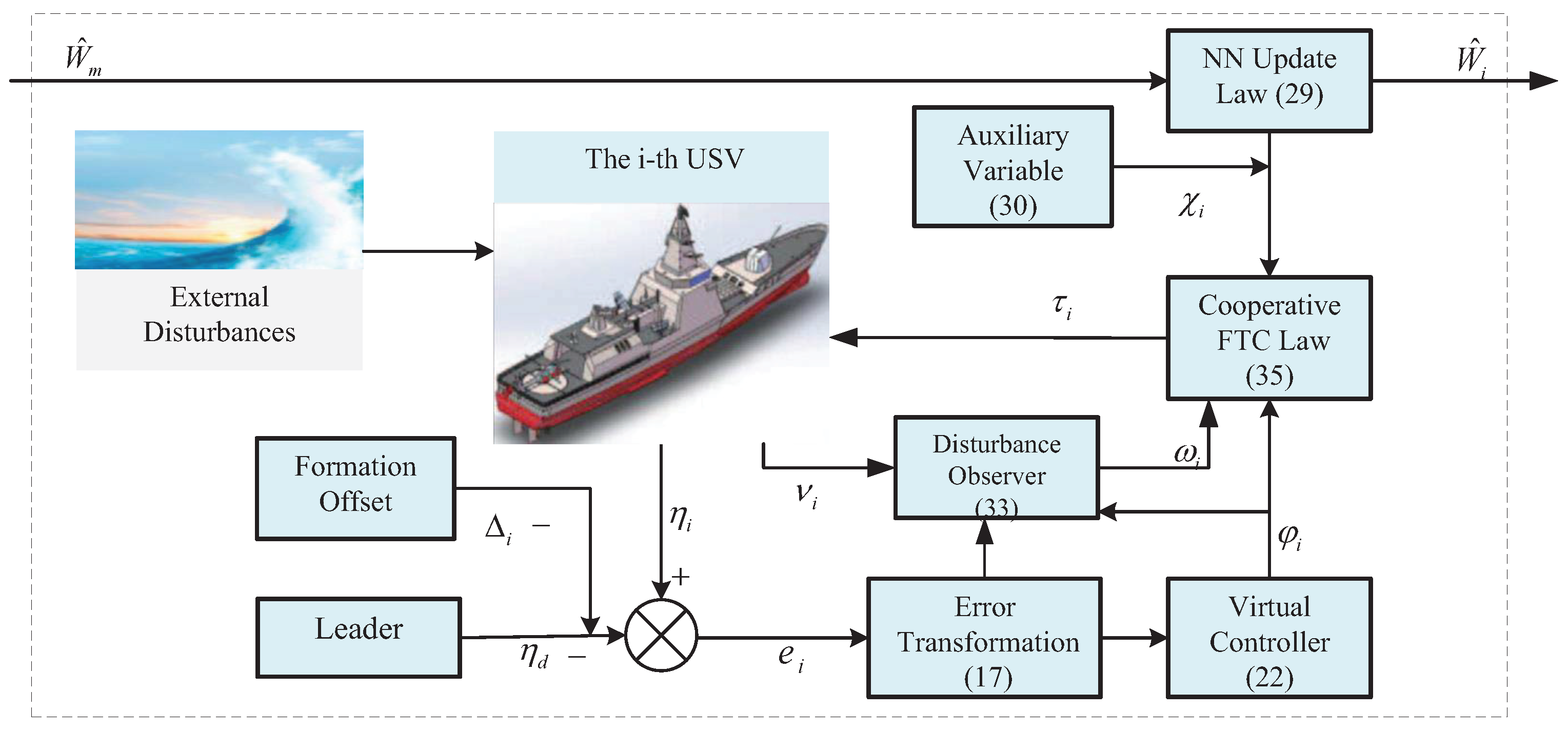
In this section, in the face of challenges encountered in practice, such as actuator faults and saturation, unknown dynamic parameters $\rho ({\eta }_i,{\nu }_i)$, and singularities in the variable actuator configuration matrix $B\left(\varphi \right)$. A formation control algorithm based on cooperative learning NNs, as shown in Figure 2, is proposed for USVs dynamics (1). It ensures adaptive tracking even in the presence of performance constraints (6), facilitating the achievement of the prescribed performance.

From (2), it can be derived that the orientation vector angle $\varphi \in {\mathbb{R}}^p$ of the propellers is divided into the following form.

$$\varphi ={\varphi }_0+∆\varphi ,$$

(11)

where ${\varphi }_0={\left[{\varphi }_{10},{\varphi }_{20},\dots ,{\varphi }_{p0}\right]}^T\in {\mathbb{R}}^p$ is the initial orientation angle of propellers, and $∆\varphi ={\left[∆{\varphi }_1,∆{\varphi }_2,\dots ,∆{\varphi }_p\right]}^T\in {\mathbb{R}}^p$ is the variable orientation angle.

By Lemma 2 and (3), we can perform the transformation

$$\begin{array}{cc}\hfill sin({\varphi }_{k0}+∆{\varphi }_k)& =sin{\varphi }_{k0}+∆{\varphi }_k{\int }_0^{1}cos({\varphi }_{k0}+s∆{\varphi }_k)ds\hfill \\ \hfill & =sin{\varphi }_{k0}+∆{\varphi }_k{\theta }_c({\varphi }_{k0},∆{\varphi }_k),\hfill \end{array}$$

(12)

$$\begin{array}{cc}\hfill cos({\varphi }_{k0}+∆{\varphi }_k)& =cos{\varphi }_{k0}-∆{\varphi }_k{\int }_0^{1}sin({\varphi }_{k0}+s∆{\varphi }_k)ds\hfill \\ \hfill & =cos{\varphi }_{k0}-∆{\varphi }_k{\theta }_s({\varphi }_{k0},∆{\varphi }_k),\hfill \end{array}$$

(13)

with bounded properties $|{\theta }_c({\varphi }_{k0},∆{\varphi }_k)|\le 1$ and $|{\theta }_s({\varphi }_{k0},∆{\varphi }_k)|\le 1$, $k=1,2,\dots ,p$.

Considering (11)–(13), we have

$$B\left(\varphi \right)=B\left({\varphi }_0\right)+∆B(∆\varphi ),$$

(14)

with

$$B\left({\varphi }_0\right)=\left[\begin{array}{cccc}cos\left({\varphi }_{10}\right)& cos\left({\varphi }_{20}\right)& \dots & cos\left({\varphi }_{p0}\right)\\ sin\left({\varphi }_{10}\right)& sin\left({\varphi }_{20}\right)& \dots & sin\left({\varphi }_{p0}\right)\\ N_{10}& N_{20}& \dots & N_{p0}\end{array}\right],$$

$$∆B(∆\varphi )=\left[\begin{array}{ccc}\hfill -∆{\varphi }_1{\theta }_s({\varphi }_{10},∆{\varphi }_1)\hfill & \hfill \dots \hfill & \hfill -∆{\varphi }_p{\theta }_s({\varphi }_{p0},∆{\varphi }_p)\hfill \\ \hfill ∆{\varphi }_1{\theta }_c({\varphi }_{10},∆{\varphi }_1)\hfill & \hfill \dots \hfill & \hfill ∆{\varphi }_p{\theta }_c({\varphi }_{p0},∆{\varphi }_p)\hfill \\ \hfill ∆N_1\hfill & \hfill \dots \hfill & \hfill ∆N_p\hfill \end{array}\right]$$

$∆N_k=l_{kx}∆{\varphi }_k{\theta }_c({\varphi }_{k0},∆{\varphi }_k)-l_{ky}∆{\varphi }_k{\theta }_s({\varphi }_{k0},∆{\varphi }_k)$, and $N_{k0}=l_{kx}sin\left({\varphi }_{k0}\right)-l_{ky}cos\left({\varphi }_{k0}\right)$.

In the coordinated operation of all propellers in tracking control, if the actuator fails, the performance of the systems will be greatly reduced, and there is even the possibility of a safety incident occurring. Therefore, designing a reasonable control plan for actuator faults is an essential step.

Assume actuator efficiency gain matrix $A\left(t\right)=diag\{a_1\left(t\right),\dots ,a_p\left(t\right)\}$, and $a_i\left(t\right)$ satisfy $0\le a_i\left(t\right)\le 1$. Then $a_i\left(t\right)$ can represent a reduction in the performance of the actuators when they are in operation. If $a_i\left(t\right)=0$, it means the i-th actuator is in a normal state. If $a_i\left(t\right)>0$, the actuator is failed, and if $a_i\left(t\right)=1$, the actuator is completely failed. $A\left(t\right)$ can be incorporated into the actuator configuration matrix. We select $K=I-A$ with $K=diag\{k_1,\dots ,k_p\}$ and $k_i=1-a_i$, then ${\tau }_{f,i}=B\left({\varphi }_0\right){\tau }_{s,i}-B\left({\varphi }_0\right)A{\tau }_{s,i}+∆B(∆\varphi )K{\tau }_{s,i}$, $0\le a_i\left(t\right)\le 1$ and $0\le 1-a_i\left(t\right)\le 1$. Therefore, we have $∥K∥<{\hslash }_1$ and $∥A∥<{\hslash }_2$ with known constants ${\hslash }_1>0$ and ${\hslash }_2>0$.

Remark 1. 

Assumption 5 is feasible, as USVs typically operate with more than three propellers, and their orientation angle vector ${\varphi }_0$ can be preset. We can select appropriate initial orientation angle to ensure that $B\left({\varphi }_0\right)$ is full row rank. Additionally, in practical USVs control systems, the deflection angle of each propeller is known to be bounded, meaning $∆{\varphi }_k$ is bounded. According to the bounded properties of ${\theta }_c({\varphi }_{k0},∆{\varphi }_k)$ and ${\theta }_s({\varphi }_{k0},∆{\varphi }_k)$, the upper bound of $∥∆B(∆\varphi )K∥$ is known with fixed $l_{kx}$ and $l_{ky}$.

Next, we perform a formal transformation of tracking error

$$e_i={\overline{e}}_i{T}_i(z_{1,i},{\chi }_{e,i}),i\in \mathcal{N},$$

(15)

where ${\chi }_{e,i}={\underline{e}}_i/{\overline{e}}_i$, the boundary functions ${\underline{e}}_i$ and ${\overline{e}}_i$ are obtained from (7). $z_{1,i}$ is the transformed error and the error transformation function $T_i(z_{1,i},{\chi }_{e,i})$ satisfies

$$\left\{\begin{array}{c}-{\chi }_{e,i}<T_i(z_{1,i},{\chi }_{e,i})<1,\forall z_{1,i}\in L_{\infty },\hfill \\ \underset{z_{1,i}\to -\infty }{lim}{T}_i(z_{1,i},{\chi }_{e,i})=-{\chi }_{e,i},\hfill \\ \underset{z_{1,i}\to +\infty }{lim}{T}_i(z_{1,i},{\chi }_{e,i})=1,\hfill \\ T_i(z_{1,i},{\chi }_{e,i})=0,if{z}_{1,i}=0,\hfill \\ {\displaystyle \frac{\partial T_i(z_{1,i},{\chi }_{e,i})}{\partial z_{1,i}}}>0,\hfill \end{array}\right.$$

(16)

where $L_{\infty }$ is a space comprising all bounded functions. The error transformation function is represented as

$$T_i(z_{1,i},{\chi }_{e,i})={\displaystyle \frac{e^{z_{1,i}}-e^{-z_{1,i}}}{e^{z_{1,i}}+{\chi }_{e,i}^{-1}{e}^{-z_{1,i}}}}.$$

(17)

Substituting (17) into (15), we have

$$z_{1,i}={\displaystyle \frac{1}{2}}ln(1+{\displaystyle \frac{e_i}{{\underline{e}}_i}})-{\displaystyle \frac{1}{2}}ln(1-{\displaystyle \frac{e_i}{{\overline{e}}_i}}),$$

and its time derivative is represented as

$${\dot{z}}_{1,i}={\gamma }_i{\dot{e}}_i-{\varpi }_i{e}_i,$$

(18)

with

$${\gamma }_i={\displaystyle \frac{1}{2}}({\displaystyle \frac{1}{{\underline{e}}_i+e_i}}+{\displaystyle \frac{1}{{\overline{e}}_i-e_i}}),{\varpi }_i={\displaystyle \frac{1}{2}}({\displaystyle \frac{{\underline{\dot{e}}}_i}{{\underline{e}}_i({\underline{e}}_i+e_i)}}+{\displaystyle \frac{{\dot{\overline{e}}}_i}{{\overline{e}}_i({\overline{e}}_i-e_i)}}).$$

Then, define ${\mathrm{\Theta }}_i=diag\left\{{\gamma }_{i1},{\gamma }_{i2},{\gamma }_{i3}\right\}$ and ${\mathrm{X}}_i=diag\left\{{\varpi }_{i1},{\varpi }_{i2},{\varpi }_{i3}\right\}$. Using (5) and (18), we can obtain

$${\dot{z}}_{1,i}={\mathrm{\Theta }}_i({\dot{\eta }}_i-{\dot{\eta }}_d-{\dot{∆}}_i)-{\mathrm{X}}_i{e}_i.$$

(19)

Based on system (1) and Equation (19) combined with the backstepping process, an adaptive formation tracking controller with the learning NNs is designed.

Step 1: Define error variable with a virtual control law ${\phi }_i$.

$$z_{2,i}={\nu }_i-{\phi }_i,$$

(20)

Substituting (1) and (20) into (19) yields

$${\dot{z}}_{1,i}={\mathrm{\Theta }}_i\left[R\left({\psi }_i\right)(z_{2,i}+{\phi }_i)-{\dot{\eta }}_d-{\dot{∆}}_i\right]-{\mathrm{X}}_i{e}_i.$$

(21)

Consider the property of system (1) with $R^T\left({\psi }_i\right)R\left({\psi }_i\right)=I$, and choose the following virtual control law

$${\phi }_i=R^T\left({\psi }_i\right)(-{\mathrm{\Theta }}_i^{-1}{\mathrm{K}}_{1,i}{z}_{1,i}+{\dot{\eta }}_d+{\dot{∆}}_i+{\mathrm{\Theta }}_i^{-1}{\mathrm{X}}_i{e}_i),$$

(22)

with ${\mathrm{\Theta }}_i^{-1}=diag\left\{1/{\gamma }_{i1},1/{\gamma }_{i2},1/{\gamma }_{i3}\right\}$ and ${\mathrm{K}}_{1,i}=diag\left\{{\kappa }_{1,i1},{\kappa }_{1,i2},{\kappa }_{1,i3}\right\}>0$.

Substituting (22) into (21), we can obtain

$${\dot{z}}_{1,i}=-{\mathrm{K}}_{1,i}{z}_{1,i}+{\mathrm{\Theta }}_{i}R\left({\psi }_i\right)z_{2,i}.$$

Consider the Lyapunov function $V_1={\displaystyle \frac{1}{2}}{\sum }_{i=1}^N{z}_{1,i}^T{z}_{1,i}$, and its time derivative is represented as

$${\dot{V}}_1={\sum }_{i=1}^N(-z_{1,i}^T{\mathrm{K}}_{1,i}{z}_{1,i}+z_{1,i}^T{\mathrm{\Theta }}_{i}R\left({\psi }_i\right)z_{2,i}),$$

(23)

where the first term in the expression gives a stable result, and the second term is analyzed through the subsequent step.

Step 2: Based on (1), the derivative of (20) is

$$\begin{array}{cc}\hfill {\dot{z}}_{2,i}=& -M^{-1}C\left({\nu }_i\right){\nu }_i-f\left(x_i\right)+{\tau }_{\omega ,i}-{\dot{\phi }}_i\hfill \\ \hfill & +M^{-1}\left[B\left({\varphi }_0\right){\tau }_{s,i}-B\left({\varphi }_0\right)A{\tau }_{s,i}+∆B(∆\varphi )K{\tau }_{s,i}\right],\hfill \end{array}$$

(24)

where ${\tau }_{\omega ,i}=M^{-1}{d}_i$ is unknown time-varying disturbance, and $f_i\left(x_i\right)$ represents the model uncertainty of the system, including the damping matrix $D\left({\nu }_i\right){\nu }_i$ and unknown dynamics $\rho ({\eta }_i,{\nu }_i)$. Therefore, $f_i\left(x_i\right)$ can be represented as

$$f_i\left(x_i\right)=M^{-1}(D\left({\nu }_i\right){\nu }_i+\rho ({\eta }_i,{\nu }_i)),$$

(25)

where $f_i\left(x_i\right)=\left[f_{i1}\left(x_i\right),f_{i2}\left(x_i\right),f_{i3}\left(x_i\right)\right]\in {\mathbb{R}}^3$ and $x_i={\left[{\eta }_i^T,{\nu }_i^T\right]}^T\in {\mathbb{R}}^6$. Then, the NNs to estimate unknown dynamics $f_{ij}\left(x_i\right),j=1,2,3$, $i\in \mathcal{N}$ are as follows.

$$f_{ij}\left(x_i\right)=W_{ij}^{*T}{h}_{ij}\left(x_i\right)+o_i\left(x_i\right)\forall x_i\in {\mathrm{\Omega }}_{x_i},$$

(26)

where $W_{ij}^{*}\in {\mathbb{R}}^l$ denotes the optimal common weight vector, and ${\mathrm{\Omega }}_{x_i}\in {\mathbb{R}}^6$ is a known compact set.

Using (24)–(26), we can obtain

$$\begin{array}{cc}\hfill {\dot{z}}_{2,i}=& -M^{-1}C\left({\nu }_i\right){\nu }_i-W_{ij}^{*T}{h}_{ij}\left(x_i\right)+{\mathrm{K}}_{d,i}{\tau }_{d,i}-{\dot{\phi }}_i\hfill \\ \hfill & +M^{-1}\left[B\left({\varphi }_0\right){\tau }_{s,i}-B\left({\varphi }_0\right)A{\tau }_{s,i}+∆B(∆\varphi )K{\tau }_{s,i}\right],\hfill \end{array}$$

(27)

where

$${\tau }_{d,i}={\mathrm{K}}_{d,i}^{-1}({\tau }_{\omega ,i}-o_i\left(x_i\right)),$$

(28)

is the sum of disturbance with ${\tau }_{d,i}={\left[{\tau }_{d,i1},{\tau }_{d,i2},{\tau }_{d,i3}\right]}^T$, and $o_i\left(x_i\right)={\left[o_{i1}\left(x_i\right),o_{i2}\left(x_i\right),o_{i3}\left(x_i\right)\right]}^T$ being the approximation error, and ${\mathrm{K}}_{d,i}=diag\left[{\kappa }_{d,i1},{\kappa }_{d,i2},{\kappa }_{d,i3}\right]>0$ being the designed parameter matrix. $W_{ij}^{*T}=diag\left[W_{i1}^{*T},W_{i2}^{*T},W_{i3}^{*T}\right]$ and $h_{ij}\left(x_i\right)={\left[h_{i1}^T\left(x_i\right),h_{i2}^T\left(x_i\right),h_{i3}^T\left(x_i\right)\right]}^T$.

Let ${\widehat{W}}_{ij}(i\in \mathcal{N},j=1,2,3)$ be the estimation of $W_{ij}$, and $W_{ij}^{*}$ be optimal common NN weight. Then, the estimation error of $W_{ij}$ is defined as ${\tilde{W}}_{ij}={\widehat{W}}_{ij}-W_{ij}^{*}$. Based on the information exchange between neighboring vehicles, cooperative NN weight update law is designed as

$$\begin{array}{cc}\hfill {\dot{\widehat{W}}}_{ij}=& -{\mathrm{Y}}_{1,i}(h_{ij}\left(x_i\right)z_{2,i}+{\sigma }_i{\widehat{W}}_{ij})\hfill \\ \hfill & -{\mathrm{Y}}_{2,i}\sum _{m=1}^n{a}_{im}({\widehat{W}}_{ij}-{\widehat{W}}_{mj}),\hfill \end{array}$$

(29)

with $i\in \mathcal{N},j=1,2,3$, ${\mathrm{Y}}_{1,i}={\mathrm{Y}}_{1,i}^T>0$, ${\sigma }_i>0$, and ${\mathrm{Y}}_{2,i}>0$ are all known parameters.

To address the potential issue of input saturation in the actuators, we design the following auxiliary system for resolution

$$\begin{array}{cc}\hfill {\dot{\chi }}_i=& -{\mathrm{\Gamma }}_i{({\mathrm{\Lambda }}_{\xi ,i}+\varsigma I_3)}^{-1}{\mathrm{\Lambda }}_c{\xi }_i\hfill \\ \hfill & -{\mathrm{\Gamma }}_i{({\mathrm{\Lambda }}_{\xi ,i}+\varsigma I_3)}^{-1}{\xi }_i{\left({\xi }_i^T{\xi }_i\right)}^{-1}\left(\right|z_{2,i}^{T}B\left({\varphi }_0\right)∆{\tau }_{s,i}|\hfill \\ \hfill & -{\hslash }_2∥z_{2,i}∥∥B\left({\varphi }_0\right)∥∥{\tau }_{s,i}∥+\beta {\hslash }_1∥z_{2,i}∥∥{\tau }_{s,i}∥),\hfill \end{array}$$

(30)

where ${\mathrm{\Gamma }}_i={(I_3-\varsigma ({\mathrm{\Lambda }}_{\xi ,i}+\varsigma I_3))}^{-1}{\xi }_i{\left({\xi }_i^T{\xi }_i\right)}^{-1}{\xi }_i^T{)}^{-1}$, ${\xi }_i={\left[{\displaystyle \frac{1}{2}}{e}^{{\chi }_{i,1}},{\displaystyle \frac{1}{2}}{e}^{{\chi }_{i,2}},{\displaystyle \frac{1}{2}}{e}^{{\chi }_{i,3}}\right]}^T\in {\mathbb{R}}^3$ is intermediate variable. $∆{\tau }_{s,i}={\tau }_{s,i}-{\tau }_i$ and ${\mathrm{\Lambda }}_{\xi ,i}=diag\left[{\displaystyle \frac{1}{2}}{e}^{{\chi }_{i,1}},{\displaystyle \frac{1}{2}}{e}^{{\chi }_{i,2}},{\displaystyle \frac{1}{2}}{e}^{{\chi }_{i,3}}\right]\in {\mathbb{R}}^{3\times 3}$. ${\mathrm{\Lambda }}_c={\mathrm{\Lambda }}_c^T>0\in {\mathbb{R}}^{3\times 3}$ and $\varsigma >0$.

Then, the derivative of ${\xi }_i$ is rewritten as

$${\dot{\xi }}_i={\mathrm{\Lambda }}_{\xi ,i}{\dot{\chi }}_i=({\mathrm{\Lambda }}_{\xi ,i}+\varsigma I_3){\dot{\chi }}_i-\varsigma {\dot{\chi }}_i.$$

(31)

Considering (30) and (31), we have

$$\begin{array}{cc}\hfill {\xi }_i^T{\dot{\xi }}_i=& -{\xi }_i^T{\mathrm{\Lambda }}_c{\xi }_i-\left(\right|z_{2,i}^{T}B\left({\varphi }_0\right)∆{\tau }_{s,i}|-{\hslash }_2∥z_{2,i}∥∥B\left({\varphi }_0\right)∥∥{\tau }_{s,i}∥+\beta {\hslash }_1∥z_{2,i}∥∥{\tau }_{s,i}∥).\hfill \end{array}$$

(32)

To estimate the unknown sum of disturbance ${\tau }_{d,i}$ in (28), we design the following distributed disturbance observer.

$$\begin{array}{cc}\hfill {\widehat{\tau }}_{d,i}& ={\omega }_i+{\mathrm{K}}_{\zeta ,i}{z}_{2,i},\hfill \\ \hfill {\dot{\omega }}_i& ={\mathrm{K}}_{d,i}{z}_{2,i}-{\mathrm{K}}_{\zeta ,i}\left[-M^{-1}C\left({\nu }_i\right){\nu }_i-{\widehat{W}}_i^{T}h\left(x_i\right)+{\mathrm{K}}_{d,i}{\widehat{\tau }}_{d,i}+M^{-1}B\left({\varphi }_0\right){\tau }_i-{\dot{\phi }}_i\right],\hfill \end{array}$$

(33)

where ${\omega }_i\in {\mathbb{R}}^3$ is the state variable of the observer and ${\mathrm{K}}_{\zeta ,i}=diag\left\{{\kappa }_{\zeta ,i1},{\kappa }_{\zeta ,i2},{\kappa }_{\zeta ,i3}\right\}>0$ is designed parameter matrix. Then, the estimation error of ${\tau }_{d,i}$ is defined as ${\tilde{\tau }}_{d,i}={\widehat{\tau }}_{d,i}-{\tau }_{d,i}$, and ${\dot{\tilde{\tau }}}_{d,i}$ is formulated as

$${\dot{\tilde{\tau }}}_{d,i}={\mathrm{K}}_{d,i}{z}_{2,i}+{\mathrm{K}}_{\zeta ,i}{\tilde{W}}_i^T{h}_i\left(x_i\right)-{\mathrm{K}}_{\zeta ,i}{\mathrm{K}}_{d,i}{\tilde{\tau }}_{d,i}-{\dot{\tau }}_{d,i}.$$

(34)

Using (29) and (33), the FTC input ${\tau }_i$ is established as

$$\begin{array}{cc}\hfill {\tau }_i=& B^{+}\left({\varphi }_0\right)[-M(R^T\left({\psi }_i\right){\mathrm{\Theta }}_i{z}_{1,i}-K_{2,i}{z}_{2,i}+{\dot{\phi }}_i\hfill \\ \hfill & +{\widehat{W}}_i^T{h}_i\left(x_i\right)-K_{d,i}{\widehat{\tau }}_{d,i}+{\xi }_i)+C\left({\nu }_i\right){\nu }_i].\hfill \end{array}$$

(35)

with $B^{+}\left({\varphi }_0\right)=B^T\left({\varphi }_0\right){\left[B\left({\varphi }_0\right)B^T\left({\varphi }_0\right)\right]}^{-1}$, and ${\mathrm{K}}_{2,i}=diag\left\{{\kappa }_{2,i1},{\kappa }_{2,i2},{\kappa }_{2,i3}\right\}$ is designed positive parameter matrix.

Substituting (35) into (27) yields

$$\begin{array}{cc}\hfill {\dot{z}}_{2,i}& =-R^T\left({\psi }_i\right){\mathrm{\Theta }}_i{z}_{1,i}-{\mathrm{K}}_{2,i}{z}_{2,i}+{\tilde{W}}_i^T{h}_i\left(x_i\right)\hfill \\ \hfill & -{\mathrm{K}}_{d,i}{\tilde{\tau }}_{d,i}+{\xi }_i+M^{-1}[B\left({\varphi }_0\right)∆{\tau }_{s,i}\hfill \\ \hfill & -B\left({\varphi }_0\right)A{\tau }_{s,i}+∆B(∆\varphi )K{\tau }_{s,i}].\hfill \end{array}$$

(36)

The Lyapunov function candidate is selected as

$$\begin{array}{cc}\hfill V_2& =V_1+{\displaystyle \frac{1}{2}}\sum _{i=1}^N\left({\xi }_i^T{M}^{-1}{\xi }_i+z_{2,i}^T{z}_{2,i}+{\tilde{\tau }}_{d,i}^T{\tilde{\tau }}_{d,i}+\sum _{j=1}^3{\tilde{W}}_{ij}^T{{\rm Y}}_{1,ij}^{-1}{\tilde{W}}_{ij}\right).\hfill \end{array}$$

(37)

Using (23), (29), (32), (34) and (36), by taking time derivative of $V_2$, we can obtain

$$\begin{array}{cc}\hfill {\dot{V}}_2& =\sum _{i=1}^N(-z_{1,i}^T{\mathrm{K}}_{1,i}{z}_{1,i}-z_{2,i}^T{\mathrm{K}}_{2,i}{z}_{2,i}-{\tilde{\tau }}_{d,i}^T{\mathrm{K}}_{\zeta ,i}{\mathrm{K}}_{d,i}{\tilde{\tau }}_{d,i}-{\tilde{\tau }}_{d,i}^T{\dot{\tau }}_{d,i}-\sum _{j=1}^3{\sigma }_{ij}{\tilde{W}}_{ij}^T{\widehat{W}}_{ij}\hfill \\ \hfill & +\sum _{j=1}^3{\mathrm{K}}_{\zeta ,ij}{\tilde{\tau }}_{d,ij}{\tilde{W}}_{ij}^T{h}_{ij}\left(x_i\right)-{\xi }_i^T{M}^{-1}{\mathrm{\Lambda }}_c{\xi }_i-|z_{2,i}^T{M}^{-1}B\left({\varphi }_0\right)∆{\tau }_s|\hfill \\ \hfill & +z_{2,i}^T{M}^{-1}\left[B\left({\varphi }_0\right)∆{\tau }_{s,i}-B\left({\varphi }_0\right)A{\tau }_{s,i}+∆B(∆\varphi )K{\tau }_{s,i}\right]\hfill \\ \hfill & +z_{2,i}^T{\xi }_i+{\hslash }_2\parallel z_{2,i}\parallel \parallel B\left({\varphi }_0\right)\parallel \parallel {\tau }_{s,i}\parallel \parallel M^{-1}\parallel quad-\beta {\hslash }_1\parallel z_{2,i}\parallel \parallel {\tau }_{s,i}\parallel \parallel M^{-1}\parallel )\hfill \\ \hfill & -\sum _{j=1}^3{{\rm Y}}_{1,j}^{-1}{{\rm Y}}_{2,j}{\tilde{W}}_j^T(L\otimes I){\tilde{W}}_j,\hfill \end{array}$$

where ${{\rm Y}}_{2,j}=\mathrm{diag}\left\{{{\rm Y}}_{2,1j},\dots ,{{\rm Y}}_{2,Nj}\right\}$, ${{\rm Y}}_{1,j}^{-1}=\mathrm{diag}\left\{{{\rm Y}}_{1,1j}^{-1},\dots ,{{\rm Y}}_{1,Nj}^{-1}\right\}$, ${{\rm Y}}_{2,j}$ and ${{\rm Y}}_{1,j}^{-1}$ are positive parameters, ${\tilde{W}}_j=\mathrm{diag}\left\{{\tilde{W}}_{1j}^T,\dots ,{\tilde{W}}_{Nj}^T\right\}$. From Assumption 1, $\mathcal{L}\otimes I$ is positive semidefinite, where I denotes an identify matrix. Then, we can obtain the following inequality

$${\displaystyle \begin{array}{c}{\dot{V}}_2\le {\displaystyle \sum _{i=1}^N}(-\underset{1,i}{\overset{T}{z}}{\mathrm{K}}_{1,i}{z}_{1,i}-z_{2,i}^T{\mathrm{K}}_{2,i}{z}_{2,i}-{\tilde{\tau }}_{d,i}^T{\mathrm{K}}_{\zeta ,i}{\mathrm{K}}_{d,i}{\tilde{\tau }}_{d,i}\hfill \\ -{\tilde{\tau }}_{d,i}^T{\dot{\tau }}_{d,i}-{\xi }_i^T{M}^{-1}{\mathrm{\Lambda }}_c{\xi }_i+z_{2,i}^T{\xi }_i\hfill \\ +{\displaystyle \sum _{j=1}^3}({\mathrm{K}}_{\zeta ,ij}{\tilde{\tau }}_{d,ij}{\tilde{W}}_{ij}^T{h}_{ij}\left(x_i\right)-{\sigma }_{ij}{\tilde{W}}_{ij}^T{\widehat{W}}_{ij})).\hfill \end{array}}$$

(38)

Based on Assumption 3 and Young’s inequality, we have

$$\begin{array}{c}-{\sigma }_{ij}{\tilde{W}}_{ij}^T{\widehat{W}}_{ij}\le -{\displaystyle \frac{1}{2}}{\sigma }_{ij}{∥{\tilde{W}}_{ij}∥}^2+{\displaystyle \frac{1}{2}}{\sigma }_{ij}{∥W_{ij}^{*}∥}^2,\hfill \\ {\mathrm{K}}_{\zeta ,ij}{\tilde{\tau }}_{d,ij}{\tilde{W}}_{ij}^T{h}_{ij}\left(x_i\right)\le {\displaystyle \frac{1}{2}}{\mathrm{K}}_{3j}{\mathrm{K}}_{\zeta ,ij}^2{h}_{ij}^{*2}{\tilde{\tau }}_{d,ij}^2+{\displaystyle \frac{{∥{\tilde{W}}_{ij}∥}^2}{2{\mathrm{K}}_{3j}}},\hfill \\ -{\tilde{\tau }}_{d,i}^T{\dot{\tau }}_{d,i}\le {\displaystyle \frac{{\kappa }_d∥{\tilde{\tau }}_{d,i}^2∥}{2}}+{\displaystyle \frac{{\overline{\tau }}_{d,i}^2}{2{\kappa }_d}},\hfill \end{array}$$

(39)

where ${\kappa }_d>0$, ${\mathrm{K}}_{3j}>0,j=1,2,3$, $\left|{\dot{\tau }}_{d,i}\right|\le {\overline{\tau }}_{d,i}$ with an unknown constant ${\overline{\tau }}_{d,i}$. By combining (39) and (38), it gives

$$\begin{array}{c}{\dot{V}}_2\le -{\displaystyle \sum _{i=1}^N}(z_{1,i}^T{\mathrm{K}}_{1,i}{z}_{1,i}+z_{2,i}^T({\mathrm{K}}_{2,i}-0.5I_{3\times 3})z_{2,i}\hfill \\ +{\displaystyle \frac{{\tilde{\tau }}_{d,i}^T{\mathrm{K}}_{\tilde{d},i}{\tilde{\tau }}_{d,i}}{2}}+{\xi }_i^T(M^{-1}{\mathrm{\Lambda }}_c-0.5I_{3\times 3}){\xi }_i\hfill \\ +{\displaystyle \sum _{j=1}^3}{\displaystyle \frac{({\sigma }_{ij}{\mathrm{K}}_{3j}-1){∥{\tilde{W}}_{ij}∥}^2}{2{\mathrm{K}}_{3j}}})+{\displaystyle \sum _{i=1}^N}({\displaystyle \sum _{j=1}^3}{\displaystyle \frac{{\sigma }_{ij}{∥W_{ij}^{*}∥}^2}{2}}+{\displaystyle \frac{{\overline{\tau }}_{d,i}^2}{2{\kappa }_d}}),\hfill \end{array}$$

(40)

where ${\mathrm{K}}_{\tilde{d},i}=\mathrm{diag}\left[2{\mathrm{K}}_{\zeta ,ij}{\mathrm{K}}_{d,ij}-{\kappa }_d-{\mathrm{K}}_{3j}{\mathrm{K}}_{\zeta ,ij}^2{h}_{ij}^{*2}\right],j=1,2,3$, ${\sigma }_{ij}{\mathrm{K}}_{3j}-1>0$ and ${\mathrm{K}}_{\tilde{d},i}>0$. Then, we can express it in the following form

$${\dot{V}}_2\le -{\zeta }_1{V}_2+{\delta }_1,$$

with

$$\begin{array}{cc}\hfill {\zeta }_1& =\underset{\begin{array}{c}i\in \mathcal{N},\\ j=1,2,3\end{array}}{min}\{2{\lambda }_{min}\left({\mathrm{K}}_{1,i}\right),{\lambda }_{min}(2{\mathrm{K}}_{2,i}-0.5I_{3\times 3}),\hfill \\ \hfill & ({\sigma }_{ij}{\mathrm{K}}_{3j}-1){\lambda }_{min}\left({{\rm Y}}_{1,ij}\right)/{\mathrm{K}}_{3j},{\lambda }_{min}\left({\mathrm{K}}_{\tilde{d},i}\right),\hfill \\ \hfill & 2{\lambda }_{min}(M^{-1}{\mathrm{\Lambda }}_c-0.5I_{3\times 3})\},\hfill \\ \hfill {\delta }_1& =\sum _{i=1}^N\left(\sum _{j=1}^3{\displaystyle \frac{{\sigma }_{ij}{\parallel W_{ij}^{*}\parallel }^2}{2}}+{\displaystyle \frac{{\overline{\tau }}_{d,i}^2}{2{\kappa }_d}}\right).\hfill \end{array}$$

In conclusion, this paper primarily focuses on the control law designed for cooperative learning NN formation control in the presence of actuator faults, input saturation, model uncertainties, and unknown external disturbances. The control law (35), NN weight update rates (29), virtual control rates (22), and disturbance observer (33) work together to keep the tracking error in specified bounds.

Theorem 1. 

For the system of USVs (1), if Assumptions 1–5 hold, based on the FTC law (35), NN weight update rate (29), and disturbance observer (33), the following conclusions for $\forall t>0,x_i\in {\mathrm{\Omega }}_{x_i}\subset R^6$ will be obtained. $\left(i\right)$ The tracking error $e_i$ never violates thresholds (6) with lower and upper bounds (7). $\left(ii\right)$ All system signals ultimately converge to a bounded state. $\left(iii\right)$ By appropriately selecting control parameters, the tracking error $e_i$, disturbance observer error ${\tilde{\tau }}_{d,i}$ can exponentially converge to a region near zero in a finite time T.

Proof. 

(i) Suppose ${\ell }_1={\displaystyle \frac{{\delta }_1}{{\zeta }_1}}$, then using (40) gives

$$V_2\left(t\right)\le (V_2\left(0\right)-{\ell }_1)exp(-{\ell }_{1}t)+{\ell }_1,\forall t\ge 0.$$

(41)

Based on (37) and (41), we can obtain

$$\begin{array}{c}∥z_{1,i}∥\le \sqrt{2{\ell }_1},∥z_{2,i}∥\le \sqrt{2{\ell }_1},\hfill \\ ∥{\tilde{W}}_i∥\le \sqrt{{\displaystyle \frac{2{\ell }_1}{{\lambda }_{min}\left({{\rm Y}}_{1,i}^{-1}\right)}}},∥{\tilde{\tau }}_{d,i}∥\le \sqrt{2{\ell }_1},\hfill \end{array}$$

(42)

thus, it implies that $z_{1,i}$, $z_{2,i}$, ${\tilde{W}}_i$ and ${\tilde{\tau }}_{d,i}$ all eventually converge to bounded states. Referring to (16), $-{\chi }_{e,i}<T_i(z_{1,i},{\chi }_{e,i})<1$, from ${\overline{e}}_i>0$, ${\chi }_{e,i}={\underline{e}}_i/{\overline{e}}_i$ and (15), we can obtain $-{\underline{e}}_i<e_i<{\overline{e}}_i$, and it proves that (6) with (7) will never be violated as $\forall t>0$.

(ii) By invoking Assumption 3 and (26), ${\tau }_{\omega ,i}$ and $o_i\left(x_i\right)$ are bounded, then ${\tau }_{d,i}$ in (28) is bounded. We know that ${\tilde{\tau }}_{d,i}={\widehat{\tau }}_{d,i}-{\tau }_{d,i}$, thus ${\widehat{\tau }}_{d,i}$ is bounded. Due to the boundedness of ${\widehat{\tau }}_{d,i}$ and $z_{2,i}$, we can obtain ${\omega }_i$ in (33) is also bounded. From Assumption 4, it is clear that the system state ${\eta }_i$ is bounded. All terms in (22) are bounded, so it can be concluded that both virtual control input ${\phi }_i$ and its derivative ${\dot{\phi }}_i$ are bounded. Using $z_{2,i}={\nu }_i-{\phi }_i$ in (20), we know that ${\nu }_i$ is bounded. In addition, the Gaussian function $h_{ij}\left(x_i\right)$ is bounded, such that all signals ultimately converge to bounded ranges.

(iii) Selected a Lyapunov function candidate as

$$V_z={\displaystyle \frac{1}{2}}\sum _{i=1}^N(z_{1,i}^T{z}_{1,i}+z_{2,i}^T{z}_{2,i}+{\xi }_i^T{M}^{-1}{\xi }_i+{\tilde{\tau }}_{d,i}^T{\tilde{\tau }}_{d,i}),$$

(43)

with its time derivative as

$$\begin{array}{cc}\hfill {\dot{V}}_z& \le \sum _{i=1}^N{\displaystyle (}-z_{1,i}^T{\mathrm{K}}_{1,i}{z}_{1,i}-z_{2,i}^T{\mathrm{K}}_{2,i}{z}_{2,i}+z_{2,i}^T{\tilde{W}}_i^T{h}_i\left(x_i\right)\hfill \\ \hfill & -{\tilde{\tau }}_{d,i}^T{\mathrm{K}}_{\zeta ,i}{\mathrm{K}}_{d,i}{\tilde{\tau }}_{d,i}+{\tilde{\tau }}_{d,i}{\mathrm{K}}_{\zeta ,i}{\tilde{W}}_i^T{h}_i\left(x_i\right)\hfill \\ \hfill & -{\tilde{\tau }}_{d,i}^T{\dot{\tau }}_{d,i}+z_{2,i}^T{\xi }_i-{\xi }_i^T{M}^{-1}{\mathrm{\Lambda }}_c{\xi }_i{\displaystyle )}.\hfill \end{array}$$

We can know from (42) that ${\tilde{W}}_i$ is bounded, then we have ${\tilde{W}}_i\le w_i^{*}$, with $w_i^{*}>0$ being an unknown constant. Using Young’s inequality, we have

$$\begin{array}{c}{z}_{2,i}{\tilde{W}}_i^T{h}_i\left(x_i\right)\le {\displaystyle \frac{1}{2}}{\overline{\mathrm{K}}}_3{z}_{2,i}^2+{\displaystyle \frac{1}{2}}{\displaystyle \frac{w{w_i^{*}}^2{h_i^{*}}^2}{{\overline{\mathrm{K}}}_3}},\hfill \\ {\mathrm{K}}_{\zeta ,i}{\tilde{\tau }}_{d,i}{\tilde{W}}_i^T{h}_i\left(x_i\right)\le {\displaystyle \frac{{\mathrm{K}}_{\zeta ,i}{\overline{\mathrm{K}}}_3{\tilde{\tau }}_{d,i}^2}{2}}+{\displaystyle \frac{{\mathrm{K}}_{\zeta ,i}{w_i^{*}}^2{h_i^{*}}^2}{2{\overline{\mathrm{K}}}_3}},\hfill \end{array}$$

(44)

with ${\overline{\mathrm{K}}}_3>0$, then using (39) and (44), we can obtain

$${\dot{V}}_z\le -{\overline{\zeta }}_1{V}_z+{\overline{\delta }}_1,$$

(45)

with

$$\begin{array}{cc}\hfill {\overline{\zeta }}_1& =\underset{\begin{array}{c}i\in \mathcal{N},\\ j=1,2,3\end{array}}{min}\{2{\lambda }_{min}\left({\overline{\mathrm{K}}}_{1,i}\right),2{\lambda }_{min}({\overline{\mathrm{K}}}_{2,i}-0.5I_{3\times 3}),\hfill \\ \hfill & {\lambda }_{min}\left(2{\overline{\mathrm{K}}}_{\tilde{d},i}\right),2{\lambda }_{min}(M^{-1}{\mathrm{\Lambda }}_c-0.5I_{3\times 3})\},\hfill \\ \hfill {\overline{\delta }}_1& =\sum _{i=1}^N\left(\sum _{j=1}^3{\displaystyle \frac{w_i^{*2}{h}_i^{*2}+{\mathrm{K}}_{\zeta ,i}{w}_i^{*2}{h}_i^{*2}}{2{\overline{\mathrm{K}}}_3}}+{\displaystyle \frac{{\overline{\tau }}_{d,i}^2}{2{\kappa }_d}}\right),\hfill \end{array}$$

where ${\overline{\mathrm{K}}}_{2,i}=\mathrm{diag}\{{\kappa }_{2,ij}-{\overline{\mathrm{K}}}_3/2\}$, ${\overline{\mathrm{K}}}_{\tilde{d},i}=\mathrm{diag}\{{\mathrm{K}}_{\zeta ,ij}{\mathrm{K}}_{d,ij}-{\kappa }_d/2-{\mathrm{K}}_{\zeta ,ij}{\overline{\mathrm{K}}}_3/2\}$. In the parameter selection, if the parameters ${\overline{\mathrm{K}}}_3$ and ${\kappa }_d$ are selected as large enough, the residual term ${\overline{\delta }}_1$ becomes small enough. We can obtain from (45) that

$$V_z\left(t\right)\le V_z\left(0\right)exp(-{\overline{\zeta }}_{1}t)+{\overline{\zeta }}_1,$$

where ${\overline{\ell }}_1={\displaystyle \frac{{\overline{\delta }}_1}{{\overline{\zeta }}_1}}$. Then, we have

$$∥z_{1,i}∥\le \sqrt{2{\overline{\ell }}_1},∥z_{2,i}∥\le \sqrt{2{\overline{\ell }}_1},∥{\tilde{\tau }}_{d,i}∥\le \sqrt{2{\overline{\ell }}_1}.$$

In summary, by appropriately selecting the control system parameters, the tracking error $e_i$, disturbance observer error ${\tilde{\tau }}_{d,i}$ can exponentially converge to a region near zero in a finite time T. The proof is completed. □

Remark 2. 

This paper highlights the difference between the proposed cooperative learning update rate (29) and the general multi-agent interaction. Through cooperative update rate, real-time knowledge and information sharing can be achieved even in the presence of actuator faults, input saturation, and model uncertainties in the dynamics of vehicles. This indicates that each vehicle can adapt its NN weight values to recognize the dynamics, where all vehicles navigate together along trajectory. Therefore, the cooperative learning NN interaction is more comprehensive and extensive compared to traditional decentralized learning.

4. Results

In this section, we validate the proposed adaptive formation tracking algorithm based on cooperative learning NNs. The USVs consists of four Cyber-ship II, which is a 1:70 scale supply vehicle. The dynamics terms of each vehicle are as follows, and the detailed model parameters of USVs are given in

Table 1. Universal hydrodynamic and nonlinear parameters.

Nonlinear Coefficients	Damping-Related Coefficients
$c_{31}=33.8v_i+1.01r_i$	$d_{11}=0.72+1.33\left|u_i\right|+5.87u_i^2$
$c_{32}=25.8u_i$	$d_{22}=0.89+36.5|u_i|+0.81|r_i|$
${\rho }_1=1+cos\left(u_i^2\right)$	$d_{23}=7.25+0.845|v_i|+3.45|r_i|$
${\rho }_2=0.01v_i^2+0.5$	$d_{32}=0.0313+3.96|v_i|+0.13|r_i|$
${\rho }_3=-0.1r_i^3+sin\left(v_i\right)$	$d_{33}=1.9-0.08|v_i|+0.75|r_i|$

.

$$M=\left[\begin{array}{ccc}25.8& 0& 0\\ 0& 33.8& 1.01\\ 0& 1.01& 2.76\end{array}\right],$$

$$C\left({\nu }_i\right)=\left[\begin{array}{ccc}0& 0& -c_{31}\\ 0& 0& -c_{32}\\ c_{31}& c_{32}& 0\end{array}\right],D\left({\nu }_i\right)=\left[\begin{array}{ccc}{d}_{11}& 0& 0\\ 0& d_{22}& d_{23}\\ 0& d_{32}& d_{33}\end{array}\right].$$

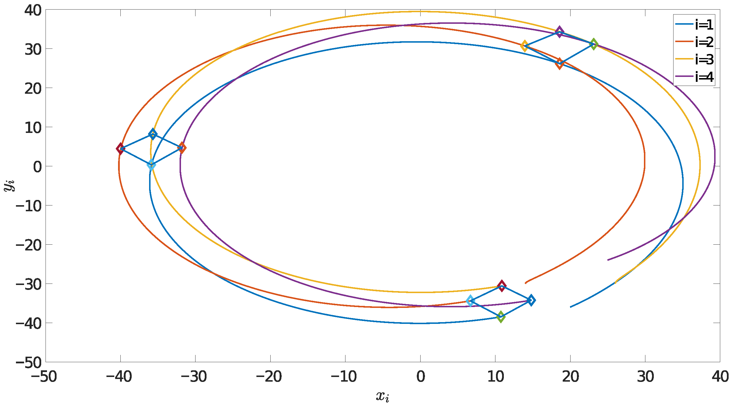
The formation tracking trajectories of the USVs in the x-y plane. The units of the position coordinates on both the $x_i$ and $y_i$ axes are in meters (m). The solid lines depict the continuous dynamic tracking paths of the four vehicles. Communication topology can be described as an adjacent set ${\mathcal{N}}_1=\{2,3\}$, ${\mathcal{N}}_2=\{1,4\}$, ${\mathcal{N}}_3=\{1,4\}$, ${\mathcal{N}}_4=\{2,3\}$. The target formation shape is a quadrilateral, and the four vehicles are located at the four vertices of the quadrilateral. Therefore, we design the position of reference trajectory as ${\eta }_d={\left[20\cos (0.1t)+30\sin (0.1t),20\sin (0.1t\right)-30\cos (0.1t),0.1t]}^T$. The designed offsets are ${∆}_1={[0,-4,0]}^T$, ${∆}_2={[-4,0,0]}^T$, ${∆}_3={[0,4,0]}^T$, and ${∆}_4={[4,0,0]}^T$. The time-varying disturbance is supposed as $d_i\left(t\right)={[5+0.6cos(0.3t+\pi /4)+1.9sin\left(0.5t\right),5+0.7sin(0.3t+\pi /6)+0.3cos\left(0.7t\right),5+0.6sin(0.8t+\pi /6)]}^T$.

The supply vehicle is controlled by four propellers, and each is responsible for controlling one of the vehicle’s orientations. The actuator parameters are ${\varphi }_{10}=-{42}^{\circ }$, ${\varphi }_{20}={42}^{\circ }$ and ${\varphi }_{30}={\varphi }_{40}={90}^{\circ }$. We that assume all the actuators are rotatable, and choose the initial configuration matrix

$$B\left({\varphi }_0\right)=\left[\begin{array}{cccc}0.7215& 0.7215& 0& 0\\ -0.6730& 0.6730& 1& 1\\ 0.3425& -0.3425& 0.3500& 0.4500\end{array}\right].$$

The parameter choices for the performance function (7) are ${\underline{e}}_{i1}={\overline{e}}_{i1}=3.7exp(-0.2t)+0.5$, ${\underline{e}}_{i2}={\overline{e}}_{i2}=2.7exp(-0.2t)+0.5$, and ${\underline{e}}_{i3}={\overline{e}}_{i3}=0.14exp(-0.2t)+0.02$ with $i=1,2,3,4$. The initial state vectors of the USVs are presented as ${\eta }_1\left(0\right)={[21,-35,0.1]}^T$, ${\eta }_2\left(0\right)={[15,-31,-0.1]}^T$, ${\eta }_3\left(0\right)={[27,-31,-0.1]}^T$, ${\eta }_4\left(0\right)={[25,-25,0.1]}^T$, and ${\nu }_i\left(0\right)={[0,0,0]}^T$. The gains of the controller are ${\mathrm{K}}_{1,i}=\mathrm{diag}\{0.3,0.3,6\}$, ${\mathrm{K}}_{2,i}=\mathrm{diag}\{3,3,6\}$, ${\mathrm{K}}_{\zeta ,i}=\mathrm{diag}\{5,9,17\}$, ${\mathrm{K}}_{d,i}=\mathrm{diag}\{2,2,2\}$, ${{\rm Y}}_{1,i1}=0.16$, ${{\rm Y}}_{1,i2}=0.44$, ${{\rm Y}}_{1,i3}=20$, ${{\rm Y}}_{2,ij}=0.5{{\rm Y}}_{1,ij},j=1,2,3$, ${\sigma }_i=0$, $\varsigma =1$, ${\mathrm{\Lambda }}_c=\mathrm{diag}\{2,2,2\}$, $\beta =10$, ${\hslash }_1=4$. The system initial values are ${\chi }_i\left(0\right)={[0,0,0]}^T$, ${\widehat{W}}_{ij}\left(0\right)=0$, ${\omega }_1\left(0\right)={[16,16,-1.20]}^T$, ${\omega }_2\left(0\right)={[21,16,-1.26]}^T$, ${\omega }_3\left(0\right)={[16,13,-1.02]}^T$, ${\omega }_4\left(0\right)={[21,13,-1.26]}^T$. The control saturation point is chosen as ${\tau }_{i,max}=150$ and ${\tau }_{i,min}=-150$.

We choose the NNs ${\widehat{W}}_{i1}^T{h}_{i1}\left(u_i\right),i=1,2,3,4$ to estimate unknown dynamics $f_1\left(u_i\right)$, and the number of neurons are 11 with the center placed in $[-2,6]$ and the width of the Gaussian function being $0.7$. Using the NNs ${\widehat{W}}_{i2}^T{h}_{i2}(v_i,r_i)$ to approximate the uncertainty $f_2(v_i,r_i)$ with 15 nodes, where the center placed in $[-0.6,2.6]\times [-2,2]$ and the width of the Gaussian function is $0.5$. Eventually, to estimate $f_3(v_i,r_i)$, we construct ${\widehat{W}}_{i3}^T{h}_{i3}(v_i,r_i)$, using 11 nodes, with the center placed in $[-0.6,2.6]\times [-2,2]$ and the width being 5.

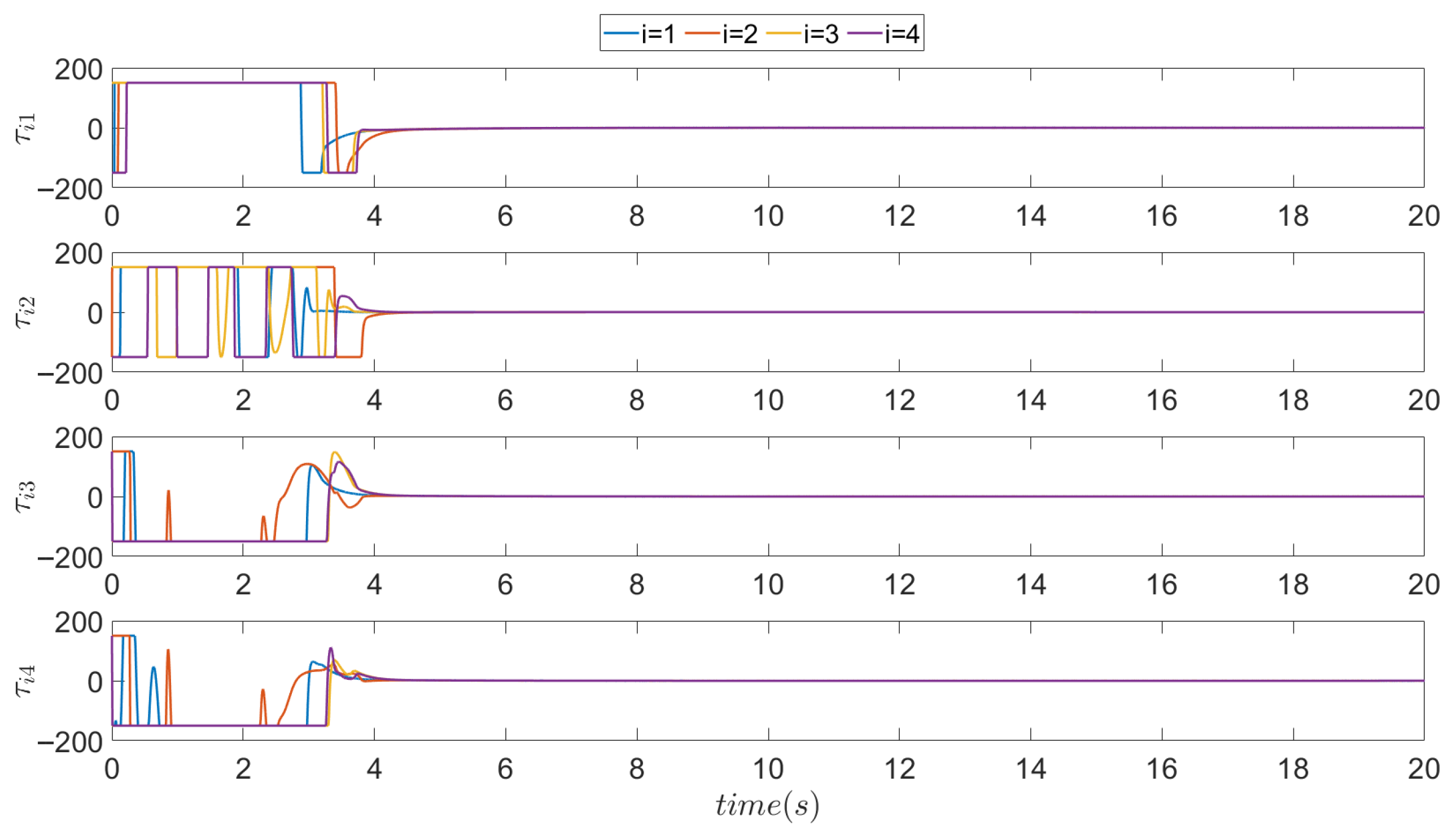
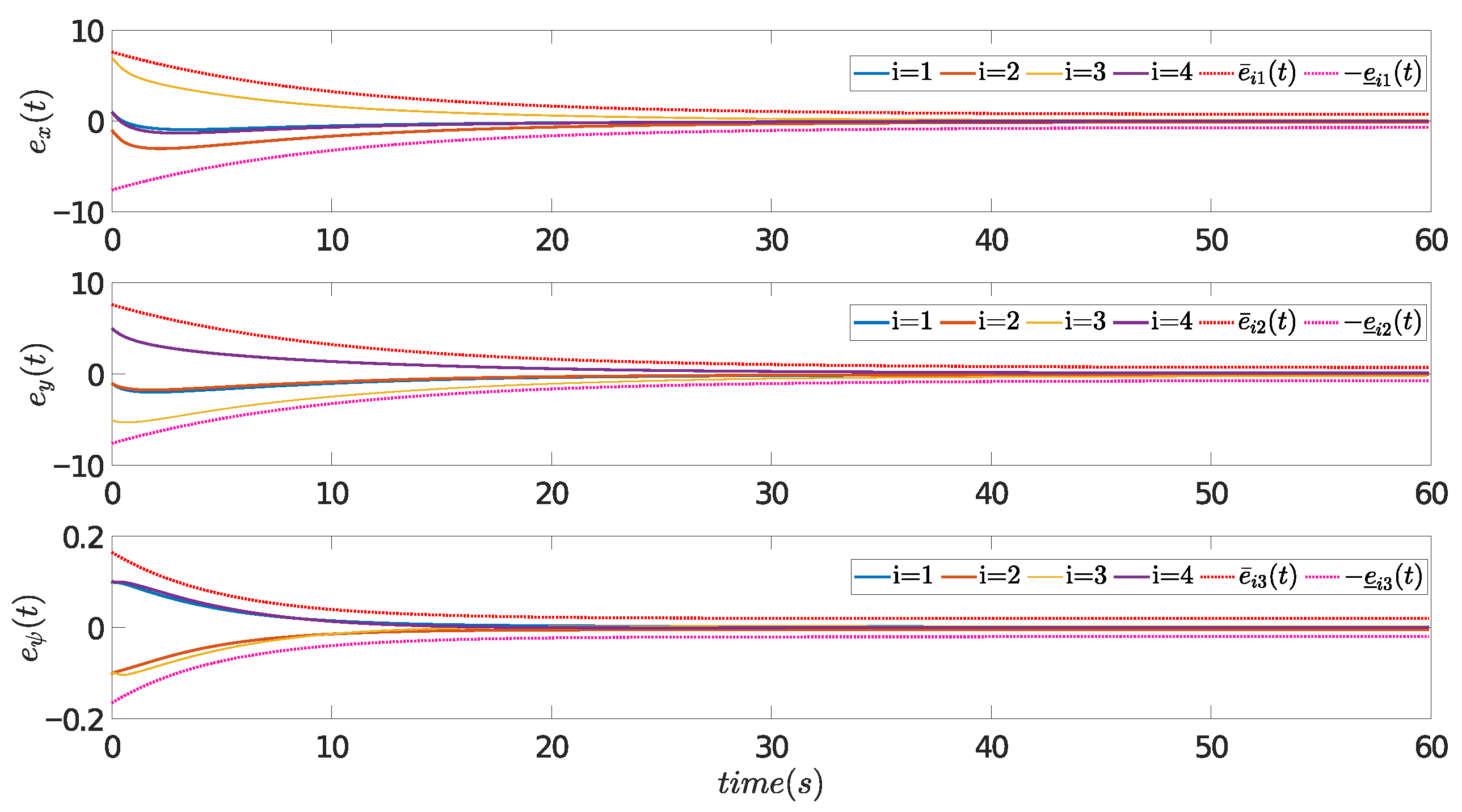
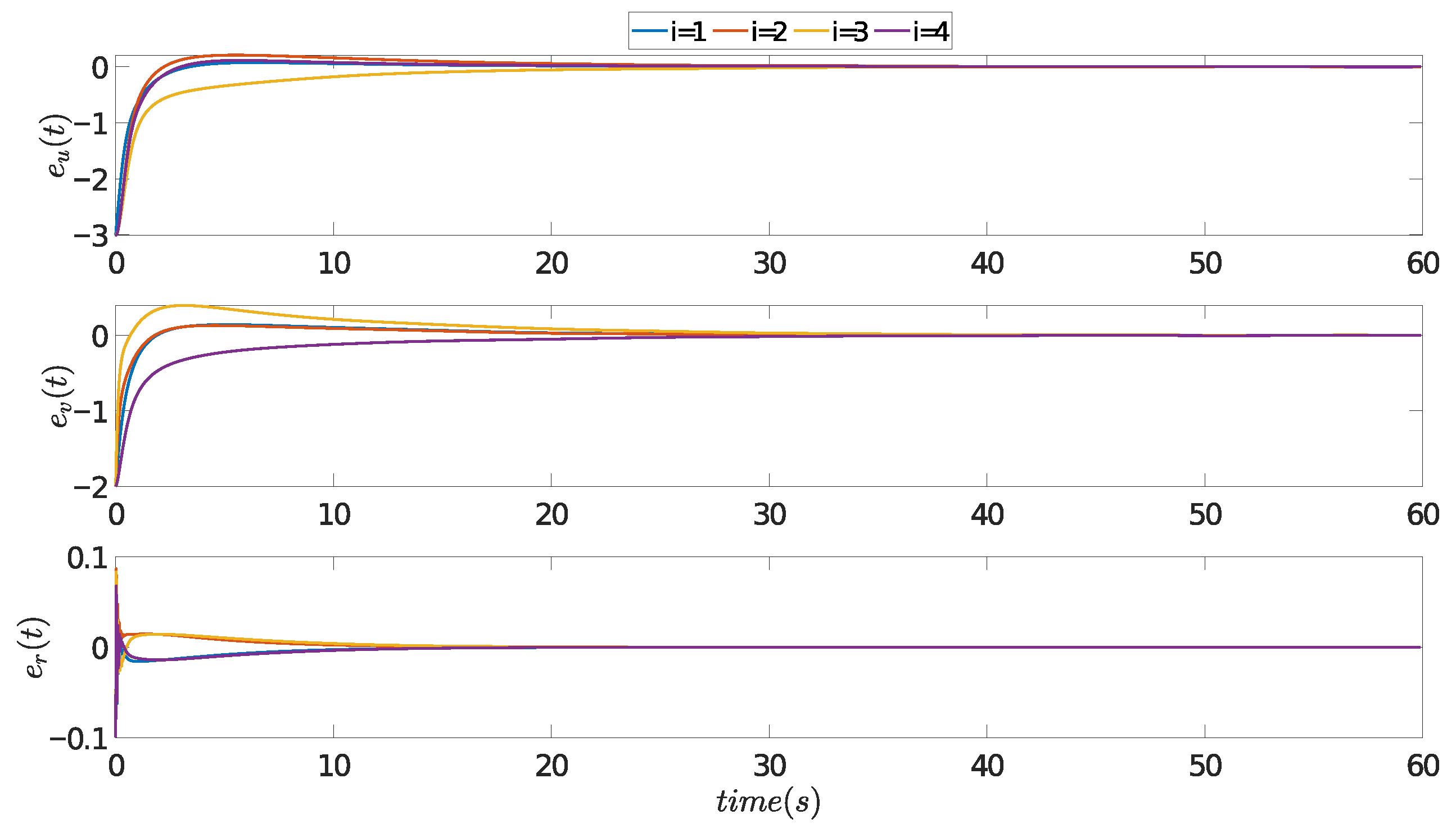
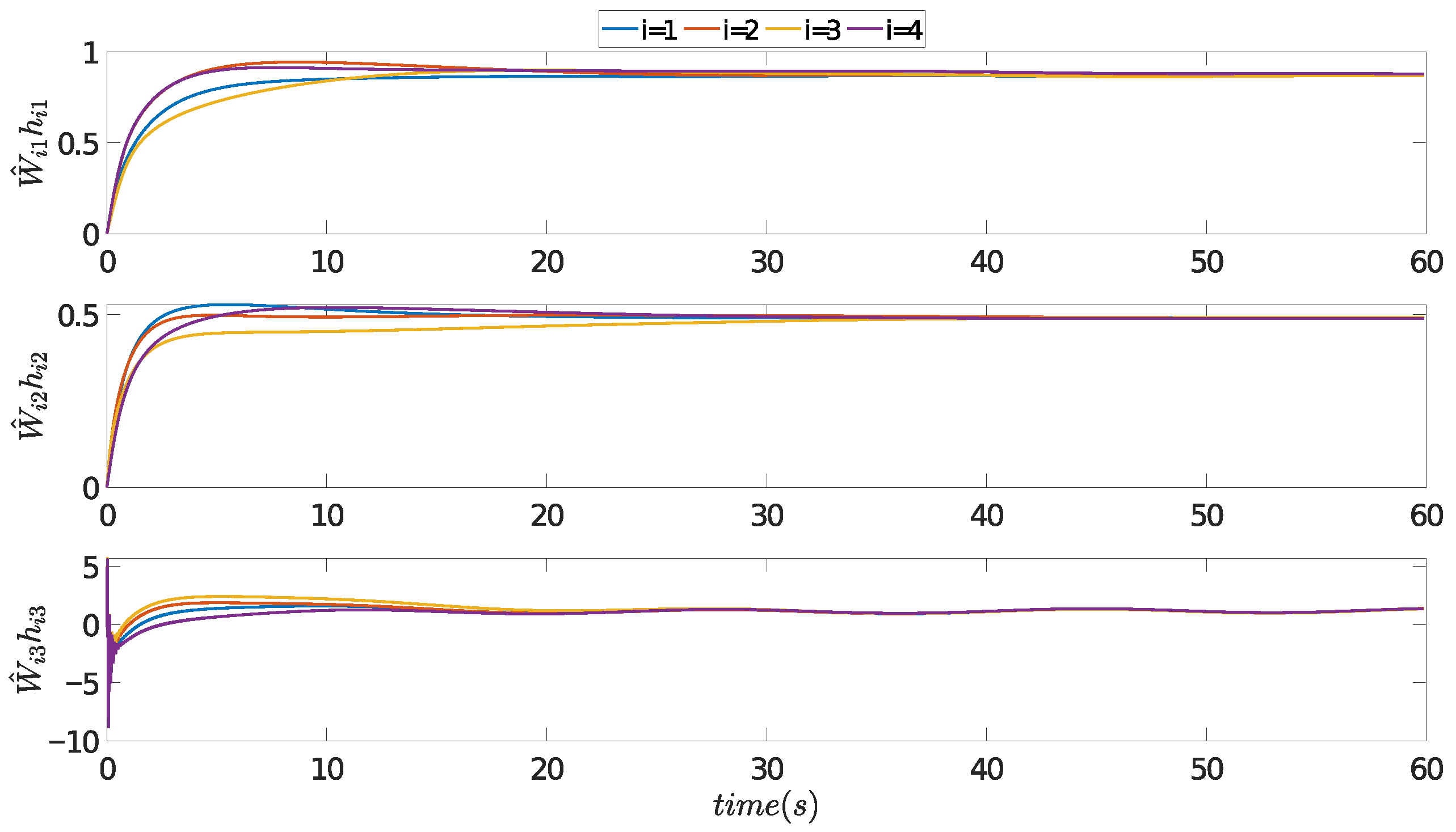
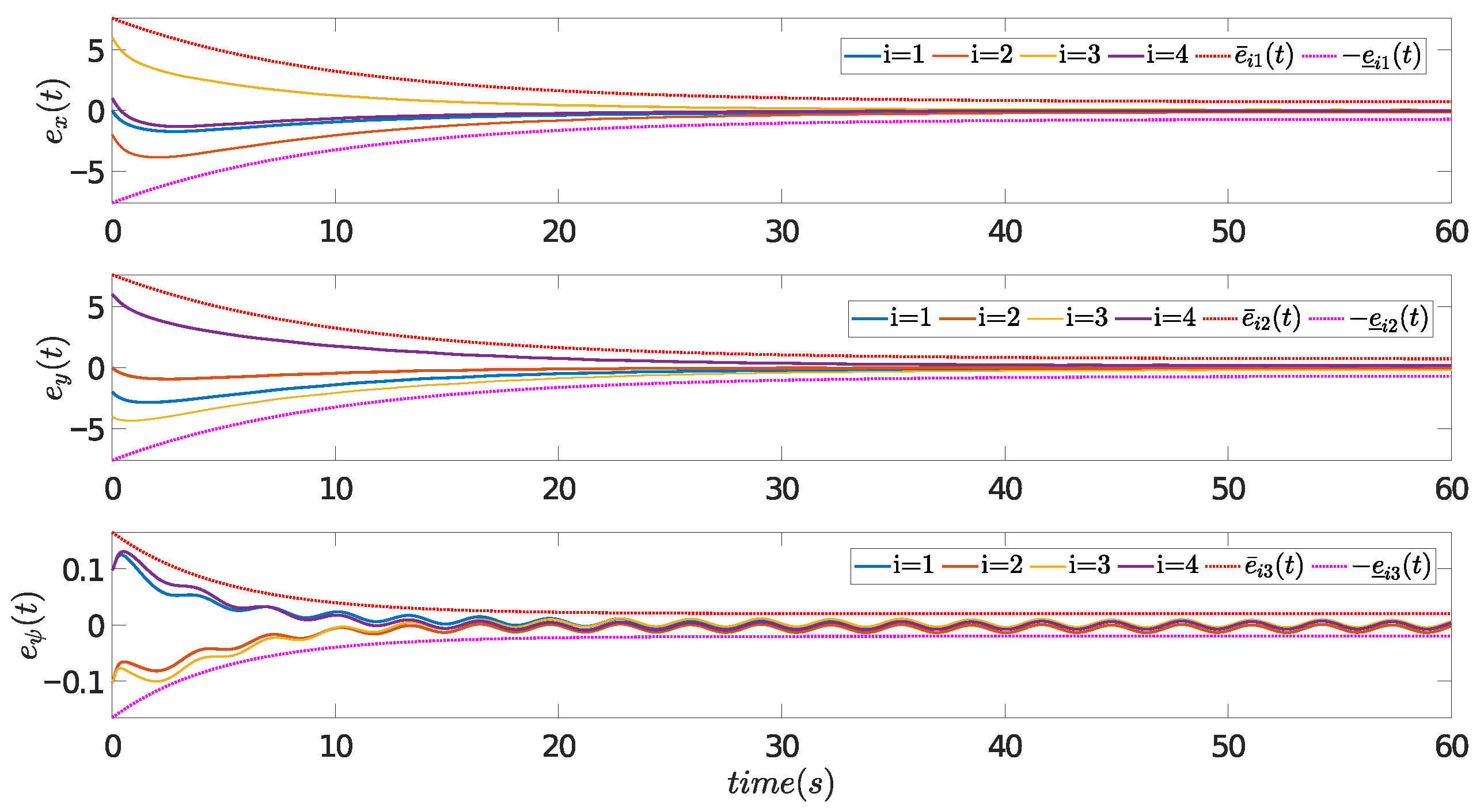
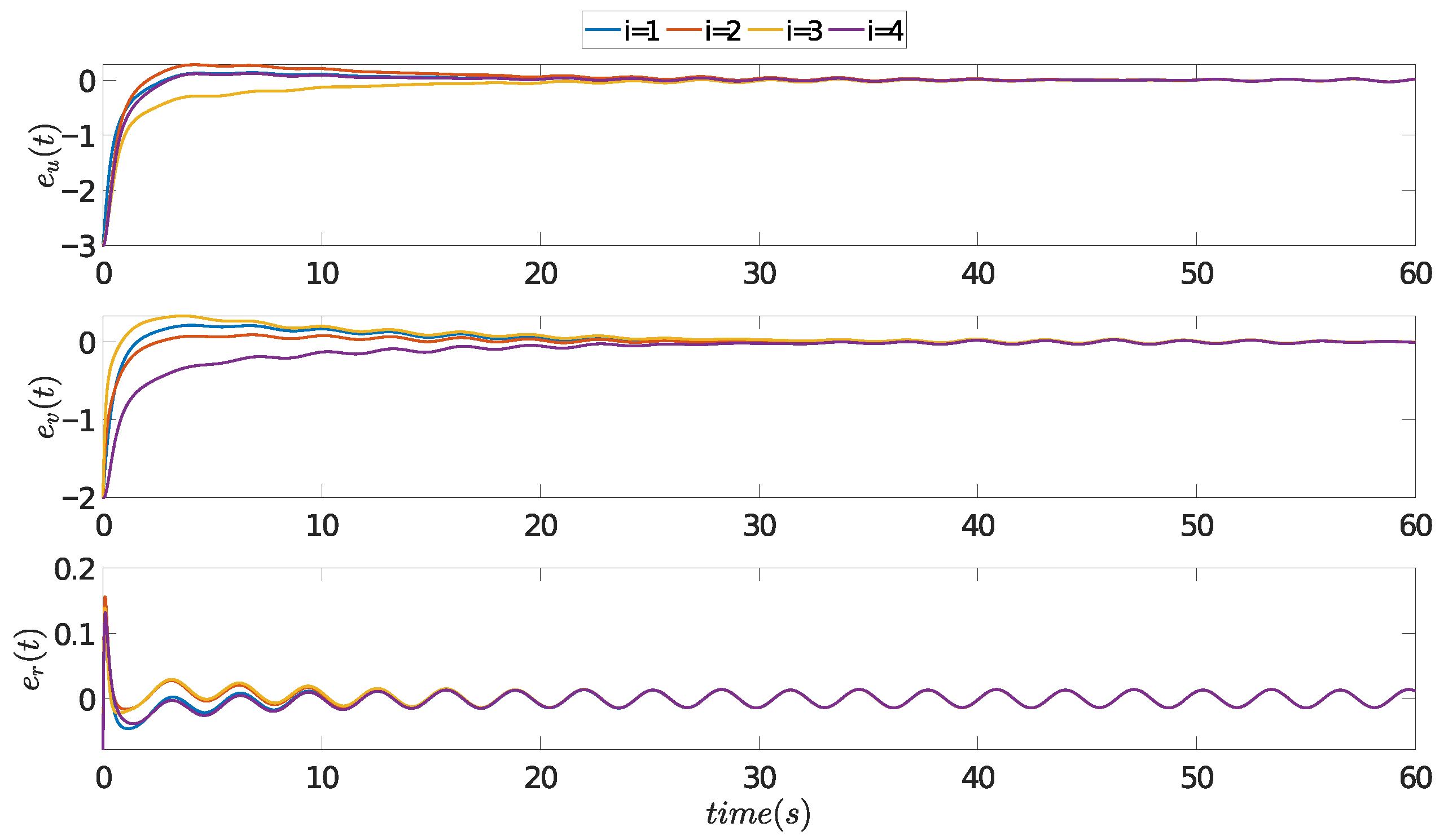
Figure 3 shows the cooperative trajectory of the USVs formation on the phase plane, where four of them can maintain a quadrilateral formation shape to complete trajectory tracking tasks.The diamond shapes denote the USVs at specific time instances, illustrating the maintenance of the desired quadrilateral formation. The tracking error curves of each USV in the formation are shown in Figure 4 and Figure 5. In the position tracking error diagram, even in the presence of model uncertainties, external disturbances, and actuator fault, the formation tracking error $e_{ij}\left(t\right)$ eventually converges to a small domain of 0 and always remains within the region formed by the prescribed performance functions ${\overline{e}}_i\left(t\right)$ and $-{\underline{e}}_i\left(t\right)$. As shown in Figure 6, the NN approximation ${\widehat{W}}_{ij}{h}_{ij}$ eventually converges together, and the designed adaptive control law with disturbance observer can identify and approximate the uncertainty of the system model. In the end, the control input signals are given by Figure 7. The tracking performance of the controllers without learning NNs in Figure 8 shows a more oscillatory and bad tracking performance. Figure 9 shows that the velocity tracking error vibration is greater without learning NNs. It shows that the traditional NNs are not able to perfectly solve formation tracking problems in the presence of model uncertainties, external disturbances, actuator faults and input saturation, while the developed control algorithm can solve the formation tracking problem of USVs systems.

To thoroughly evaluate the robustness and superiority of the proposed cooperative learning FTC algorithm, an in-depth analysis of the system’s response to external disturbances, model uncertainties, actuator faults, and input saturation is conducted below.

External Disturbances: Despite the continuous injection of complex, time-varying environmental disturbances, the position and velocity tracking errors of the formation (Figure 4 and Figure 5) converge rapidly. Driven by the distributed disturbance observer, the tracking errors $e_{ij}\left(t\right)$ are strictly constrained within the predefined upper and lower boundaries of the prescribed performance functions, ${\overline{e}}_i\left(t\right)$ and $-{\underline{e}}_i\left(t\right)$. This demonstrates the observer’s capability to provide accurate real-time compensation, ensuring high-precision formation keeping under harsh marine conditions.

Model Uncertainties: The learning and adaptive capabilities of the proposed method are validated in Figure 6, where the neural network approximation terms ${\widehat{W}}_{ij}^T{h}_{ij}\left(x_i\right)$ stabilize after an initial transient phase, effectively identifying the unknown nonlinear dynamics. The critical advantage of this cooperative learning mechanism becomes distinctly visually evident when comparing the proposed method (Figure 4 and Figure 5) with the non-learning traditional NN approach (Figure 8 and Figure 9). The absence of cooperative learning NNs in Figure 8 and Figure 9 leads to continuous, severe oscillations and degraded steady-state performance in tracking errors. Conversely, the proposed method completely mitigates these oscillations, proving its superior ability to handle unmodeled dynamics.

Actuator Faults: In practical USV operations, actuator efficiency loss severely threatens system stability. Figure 7 illustrates the dynamic evolutions of the FTC control inputs ${\tau }_i$. Upon the occurrence of simulated actuator faults during the operation, the designed fault-tolerant control law (Equation (35)) automatically and rapidly reallocates the control signals. This instantaneous restructuring of the control inputs guarantees that the multi-agent system continues to generate sufficient and balanced forces to maintain the target quadrilateral formation, thereby preventing the destabilization that typically follows propeller failures.

Input Saturation: To ensure physical realizability, the control inputs must strictly adhere to the mechanical limitations of the actuators. As clearly depicted in Figure 7, all control input signals are safely confined within the predefined saturation boundaries of $\pm 150$, even during initial transient responses or post-fault signal reallocations. The introduced adaptive auxiliary system actively compensates for the nonlinear effects induced by control truncation. By successfully averting the integral wind-up phenomenon, the system maintains the prescribed tracking performance without violating the physical constraints of the USVs.

5. Conclusions

This article investigates a cooperative learning control strategy with prescribed performance to address the formation tracking problem of unmanned surface vehicles (USVs) subject to model uncertainties, external disturbances, actuator faults, and input saturation. By integrating learning neural networks (NNs) for approximating unknown dynamics, distributed disturbance observers, and the backstepping technique, a novel fault-tolerant formation control algorithm is proposed. In this framework, each vehicle utilizes a cooperative learning update law to adjust its NN weights, enabling the recognition and sharing of learned information across the multi-agent network. Consequently, the proposed method significantly enhances the control system’s tracking performance and strictly maintains the formation errors within the prescribed performance bounds. Furthermore, rigorous convergence analysis based on the Lyapunov method theoretically guarantees the stability of the closed-loop system.

Despite the demonstrated effectiveness, the present study has certain limitations that should be explicitly acknowledged. First, the current theoretical findings are validated exclusively through numerical simulations and have not yet been verified by hardware implementations or sea-trial experiments. Second, the cooperative control protocol is designed under a fixed and connected communication topology, whereas practical marine operations frequently involve more complex, switching, or partially disrupted communication environments. Third, the considered actuator fault model primarily focuses on loss of effectiveness combined with input saturation phenomena; more complicated actuator failure modes and sensor-side uncertainties are not addressed in this work. Finally, the controller design relies on the assumption that the reference trajectory and the main system states are continuously available and sufficiently smooth.

To address these limitations, future research will focus on extending the proposed control framework to accommodate more complex and realistic operating conditions. Specifically, we aim to investigate resilient cooperative control strategies under switching communication topologies and network-induced cyberattacks or disturbances. Additionally, accommodating measurement noise and conducting experimental validations on a physical USV platform will be critical steps in our subsequent studies to further verify the practical applicability of the proposed algorithm.

References

1. Cao, L.; Pan, Y.; Liang, H.; Ahn, C.K. Event-based adaptive neural network control for large-scale systems with nonconstant control gains and unknown measurement sensitivity. IEEE Trans. Syst. Man Cybern. Syst. 2024, 54, 7027–7038. [Google Scholar] [CrossRef] [Scilit]
2. Cai, W.; Ju, Y.; Liu, Z.; Zhang, M.; Lv, S. Event-triggered leader-follower communication based formation control with dual-predictor for multiple AUVs. Ocean Eng. 2025, 334, 121552. [Google Scholar] [CrossRef] [Scilit]
3. Chen, G.; Dong, J. Approximate optimal adaptive prescribed performance fault-tolerant control for autonomous underwater vehicle based on self-organizing neural networks. IEEE Trans. Veh. Technol. 2024, 73, 9776–9785. [Google Scholar] [CrossRef] [Scilit]
4. Chang, Z.; Yao, X.; Zhang, Y.; Park, J.H. Multi-layer NN-based fixed-time distributed optimisation for coordinated dynamic positioning of unmanned surface vehicles. Int. J. Control 2025, 99, 966–984. [Google Scholar] [CrossRef] [Scilit]
5. Zhang, J.; Yuan, C.; Wu, F.; Wang, C.; Cheng, H. Deterministic learning-based tracking control for parabolic PDE systems with infinite-dimensional nonlinear uncertain dynamics. IEEE Trans. Autom. Control 2025, 70, 3272–3287. [Google Scholar] [CrossRef] [Scilit]
6. Zhao, J.; Lin, Y. Adaptive actuator failure compensation control: A new scheme based on fault detection and isolation. IEEE/ASME Trans. Mechatron. 2023, 28, 2236–2247. [Google Scholar] [CrossRef] [Scilit]
7. Zhou, S.; Wei, Y.; Cao, J.; Liu, Y. Multi/Single-Stage sliding manifold approaches for prescribed-time distributed optimization. IEEE Trans. Autom. Control 2025, 70, 2794–2801. [Google Scholar] [CrossRef] [Scilit]
8. Wen, L.; Zhang, X.; Chen, Y.; Li, T.; Wang, Q. Composite-observer-based adaptive consensus tracking control for nonlinear MASs with unknown control directions against deception attacks. IEEE Trans. Cybern. 2025, 55, 343–354. [Google Scholar] [CrossRef] [Scilit]
9. Ding, T.; Zhang, H.; Ge, M.; Cao, W.; Liu, Z. Secure formation tracking of networked MSVs under actuator constraints and DoS attacks: Data-driven observer-based control. IEEE Trans. Intell. Veh. 2025, 10, 1414–1426. [Google Scholar] [CrossRef] [Scilit]
10. Ge, S.S.; Wang, C. Adaptive neural control of uncertain MIMO nonlinear systems. IEEE Trans. Neural Netw. 2004, 15, 674–692. [Google Scholar] [CrossRef] [Scilit]
11. Guo, X.; Cui, R.; Yan, W. Pursuit-evasion games of marine surface vessels using neural network-based control. IEEE Trans. Syst. Man Cybern. Syst. 2025, 55, 18–27. [Google Scholar] [CrossRef] [Scilit]
12. Hu, W.; Shao, S.; An, Z.; Chen, M. Prescribed performance discrete-time fuzzy carrier landing control of UAV based on disturbance observer. Int. J. Fuzzy Syst. 2023, 25, 3074–3088. [Google Scholar] [CrossRef] [Scilit]
13. Liu, D.; Mao, Z.; Jiang, B.; Yan, X.-G. Prescribed performance fault-tolerant control for synchronization of heterogeneous nonlinear MASs using reinforcement learning. IEEE Trans. Cybern. 2024, 54, 5451–5462. [Google Scholar] [CrossRef] [Scilit] [PubMed]
14. Jiang, J.; Jin, X.; Xie, X.; Wang, H. Nonlinear ELM estimator-based formation control for perturbed unmanned surface vehicle systems with prescribed performance. IEEE Trans. Intell. Veh. 2024, 9, 8175–8189. [Google Scholar] [CrossRef] [Scilit]
15. Johansen, T.A.; Fuglseth, T.P.; Tøndel, P.; Fossen, T.I. Optimal constrained control allocation in marine surface vessels with rudders. Control Eng. Pract. 2008, 16, 457–464. [Google Scholar] [CrossRef] [Scilit]
16. Krstic, M.; Bhan, L.; Shi, Y. Neural operators of backstepping controller and observer gain functions for reaction–diffusion PDEs. Automatica 2024, 164, 111649. [Google Scholar] [CrossRef] [Scilit]
17. Li, K.; Feng, K.; Li, Y. Fuzzy adaptive fault-tolerant formation control for USVs with intermittent actuator faults. IEEE Trans. Intell. Veh. 2024, 9, 4445–4455. [Google Scholar] [CrossRef] [Scilit]
18. Liang, Z.; Shen, M.; Li, Z.; Yang, J. Model-free output feedback path following control for autonomous vehicle with prescribed performance independent of initial conditions. IEEE/ASME Trans. Mechatron. 2024, 29, 1076–1087. [Google Scholar] [CrossRef] [Scilit]
19. Liu, S.; Zhang, R.; Zhao, D.; Song, H. Adaptive dual-channel event-triggered fuzzy control for autonomous underwater vehicles with multiple obstacles environment. IEEE Trans. Intell. Transp. Syst. 2024, 25, 14816–14829. [Google Scholar] [CrossRef] [Scilit]
20. Xiao, Y.; Yuan, Y.; Yang, C.; Luo, B.; Xu, X.; Dubljevic, S. Adaptive neural tracking control of a class of hyperbolic PDE with uncertain actuator dynamics. IEEE Trans. Cybern. 2024, 54, 693–705. [Google Scholar] [CrossRef] [Scilit]
21. Ma, Y.; Zhang, K.; Jiang, B. Neuroadaptive cooperative fault-tolerant control of heterogeneous multiagent systems based on fully actuated system approaches. IEEE Trans. Cybern. 2023, 54, 4581–4592. [Google Scholar] [CrossRef] [Scilit]
22. Qiu, H.; Korovin, I.; Liu, H.; Gorbachev, S.; Gorbacheva, N.; Cao, J. Distributed adaptive neural network consensus control of fractional-order multi-agent systems with unknown control directions. Inf. Sci. 2024, 655, 119871. [Google Scholar] [CrossRef] [Scilit]
23. Skjetne, R.; Fossen, T.I.; Kokotović, P.V. Adaptive maneuvering, with experiments, for a model ship in a marine control laboratory. Automatica 2005, 41, 289–298. [Google Scholar] [CrossRef] [Scilit]
24. Tsolakis, A.; Negenborn, R.R.; Reppa, V.; Ferranti, L. Model predictive trajectory optimization and control for autonomous surface vessels considering traffic rules. IEEE Trans. Intell. Transp. Syst. 2024, 25, 9895–9908. [Google Scholar] [CrossRef] [Scilit]
25. Wang, D.; Ge, S.; Liang, X.; Li, D. Time-synchronized formation control of unmanned surface vehicles. IEEE Trans. Intell. Veh. 2024, 9, 6567–6575. [Google Scholar] [CrossRef] [Scilit]
26. Liu, Q.; Zhang, K.; Jiang, B. Fixed-time fault estimation and prescribed performance fault-tolerant control for interconnected systems. IEEE Trans. Cybern. 2024, 54, 1084–1095. [Google Scholar] [CrossRef] [Scilit] [PubMed]
27. Wang, Y.; Zhang, M.; Tian, S.; Lu, C.; Wu, M.; Sato, D. An adaptive integral sliding mode control-based amplitude and phase compensation repetitive control method. IEEE Trans. Ind. Electron. 2024, 71, 16644–16653. [Google Scholar] [CrossRef] [Scilit]
28. Wang, Z.; Guo, Z.; Li, S. Finite-time disturbance rejection control for rigid spacecraft attitude set stabilization with actuator saturation. IEEE Trans. Aerosp. Electron. Syst. 2024, 60, 4910–4922. [Google Scholar] [CrossRef] [Scilit]
29. Yan, Y.; Yu, S.; Gao, X.; Wu, D.; Li, T. Continuous and periodic event-triggered sliding-mode control for path following of underactuated surface vehicles. IEEE Trans. Cybern. 2024, 54, 449–461. [Google Scholar] [CrossRef] [Scilit]
30. Miao, Q.; Zhang, K.; Jiang, B. Fixed-time collision-free fault-tolerant formation control of multi-UAVs under actuator faults. IEEE Trans. Cybern. 2024, 54, 3679–3691. [Google Scholar] [CrossRef] [Scilit]
31. Wang, N.; Gao, Y.; Zhao, H.; Ahn, C.K. Reinforcement learning-based optimal tracking control of an underactuated surface vehicle with unknown dynamics. IEEE Trans. Neural Netw. Learn. Syst. 2021, 32, 3058–3069. [Google Scholar] [CrossRef] [Scilit] [PubMed]
32. Cui, R.; Ge, S.; How, B.V.E.; Choo, Y.S. Leader-follower formation control of underactuated autonomous underwater vehicles. Ocean Eng. 2010, 37, 1491–1520. [Google Scholar] [CrossRef] [Scilit]
33. Chen, T.; Zhu, Z.; Wang, C. Rapid sensor fault diagnosis for a class of nonlinear systems via deterministic learning. IEEE Trans. Neural Netw. Learn. Syst. 2023, 34, 8594–8608. [Google Scholar] [CrossRef] [Scilit] [PubMed]
Figure 1. The definition of earth-fixed and body-fixed coordinate of the vehicle.
Machines 14 00452 g001
Figure 2. General framework of the control scheme.
Machines 14 00452 g002
Figure 3. The formation tracking trajectories of the USVs. The diamond shapes denote the USVs at specific time instances, illustrating the maintenance of the desired quadrilateral formation.
Machines 14 00452 g003
Figure 4. The evolution of the position tracking errors e i j .
Machines 14 00452 g004
Figure 5. The evolution of the velocity tracking errors e ˙ i j .
Machines 14 00452 g005
Figure 6. NN approximation W ^ i j h i j ( x i ) with the disturbance-observer.
Machines 14 00452 g006
Figure 7. The evolutions of FTC input τ i .
Machines 14 00452 g007
Figure 8. The position tracking errors e i j without learning NNs.
Machines 14 00452 g008
Figure 9. The velocity tracking errors e ˙ i j without learning NNs.
Machines 14 00452 g009