Fourier-Encoded Plücker Line Fields for Globally Bounded Inverse Velocity Mapping of Axisymmetric Parallel Mechanisms

Abstract

To address inverse-velocity amplification and numerical instability of axisymmetric parallel mechanisms near dead-point regions, this paper proposes a low-dimensional feature representation and stable inverse-solving framework based on Fourier-encoded Plücker line fields. The limb axes are first represented by normalized Plücker line vectors, and the discrete rod-axis set is lifted to a circumferential continuous line field. A compact feature vector composed of first-order Fourier coefficients is then constructed, from which the continuous feature coefficients and the corresponding feature Jacobian are derived in closed form. Under constant-length constraints, feasible sensitivity and worst-case gain are introduced to characterize local inverse amplification, and a weighted damped KKT inverse solver is formulated to obtain globally bounded inverse solutions for feature velocities. Numerical results show that, in the ideal axisymmetric model, higher-order harmonics remain at numerical-residual levels and the first-order truncation stays dominant, while the most unfavorable amplification location is governed by the trough of feasible sensitivity. For fully reachable targets, the proposed solver reduces the peak generalized velocity by about 4.32%. For targets containing unreachable components, the damped KKT inverse introduces only a small additional residual while keeping the velocity bounded. Additional tests under mild geometric perturbations show that non-ideal errors mainly affect low-order fitting accuracy and higher-order spectral leakage, whereas the peak worst-case gain and the peak-shaving ratio remain largely stable. These results demonstrate that the proposed framework provides a unified description for inverse velocity mapping of axisymmetric parallel mechanisms with analytical interpretability, global boundedness, and robustness under mild geometric imperfections.

1. Introduction

Parallel mechanisms play an important role in parallel machine tools, high-speed operation platforms, and testing or docking systems because their closed-loop architectures provide high stiffness, high load capacity, and high positioning accuracy [1,2,3,4,5]. At the same time, their closed-chain nature also brings challenging kinematic issues, especially near singular or ill-conditioned configurations, where motion/force transmission and inverse mapping can deteriorate significantly [6,7,8,9]. As advanced engineering systems increasingly demand both high dynamic performance and high precision, the quality of kinematic mapping over the entire workspace directly affects control performance, trajectory-planning efficiency, and overall engineering usability. Developing a modeling and inverse-solving framework that is both geometrically interpretable and numerically stable has therefore become a fundamental issue in high-performance applications of parallel mechanisms.

Screw theory and line geometry provide a unified geometric language for parallel mechanisms [10,11,12,13,14,15,16]. By using twists, wrenches, and Plücker line coordinates, rigid-body instantaneous motion, constraints, and force transmission can be described within a common framework under closed-loop conditions. Along this route, several studies have used screw- and line-based formulations for Jacobian construction and performance analysis. For example, Wang et al. developed a generalized Jacobian for nonredundant parallel manipulators by means of repelling screws [14], whereas Meng et al. employed screw theory to analyze the motion/force transmissibility of high-speed parallel robots [17]. In addition, Wolf et al. investigated singular configurations and neighboring singular behavior of the 3-DOF CaPaMan manipulator using line geometry and linear complex approximation [18]; Zhao et al. analyzed the physical meaning of singularity in spatial parallel manipulators through terminal constraints and reciprocal screws [19]; and Han and Liu further established the geometric relationship between singular configurations and singular kinematic screws in a 3UPS-S parallel mechanism [20]. These studies have advanced Jacobian construction, singularity analysis, and screw-based physical interpretation. However, they do not provide a compact circumferential feature representation tailored to axisymmetric multi-limb parallel mechanisms, nor do they establish a unified analytical framework that directly connects local inverse amplification with bounded inverse-velocity solutions.

On the numerical side, several singularity-robust strategies have been proposed, including dimensionally homogeneous Jacobians [21], singularity-robust inverse solutions [22], and singularity-robust inverse kinematics via reparameterization [23]. These methods substantially improve conditioning or numerical stability in ill-conditioned regions. However, for axisymmetric parallel mechanisms, a unified formulation is still lacking that simultaneously preserves the geometric meaning of the limb-axis set, enables analytical differentiation in a low-dimensional feature space, and supports stable inverse-velocity computation.

Motivated by this gap, this paper proposes a low-dimensional feature representation and stable inverse-solving framework for an axisymmetric multi-limb parallel mechanism based on Fourier-encoded Plücker line fields. Each limb axis is represented by a normalized Plücker line vector, and the discrete rod-axis set is lifted to a circumferential continuous line field. A compact feature vector composed of first-order Fourier coefficients is then constructed, from which the continuous coefficient curves and the analytical feature Jacobian are derived in closed form. Under constant-length constraints, the admissible generalized velocity at any pose is shown to lie in a one-dimensional subspace, which motivates the definition of feasible sensitivity and its associated worst-case gain for characterizing local inverse amplification. A weighted damped KKT inverse solver is finally formulated to obtain globally bounded inverse-velocity responses.

The main contributions of this work are summarized as follows.

(1) An exact first-order low-dimensional representation of the normalized Plücker line field is established under ax-isymmetry, together with closed-form coefficient curves and an analytical feature Jacobian.

(2) The relationships among dead points, feasible sensitivity, local inverse amplification, and the most unfavorable pose are clarified through a feasible-sensitivity-based interpretation.

(3) A globally bounded and stable inverse-solving framework is constructed and validated through tests involving reachable targets, targets with unreachable components, and mild geometric perturbations.

The remainder of this paper is organized as follows. Section 2 establishes the line-field feature model for the ax-isymmetric mechanism and derives the analytical coefficients, feature Jacobian, and stable inverse formulation. Section 3 presents numerical experiments on coefficient recovery, harmonic decay, inverse amplification, and ro-bustness under mild geometric perturbations. Section 4 provides the discussion and conclusions.

2. Line-Field Feature Modeling and Stable Inverse Mapping Method

2.1. Geometric Model and Constraints of the Mechanism

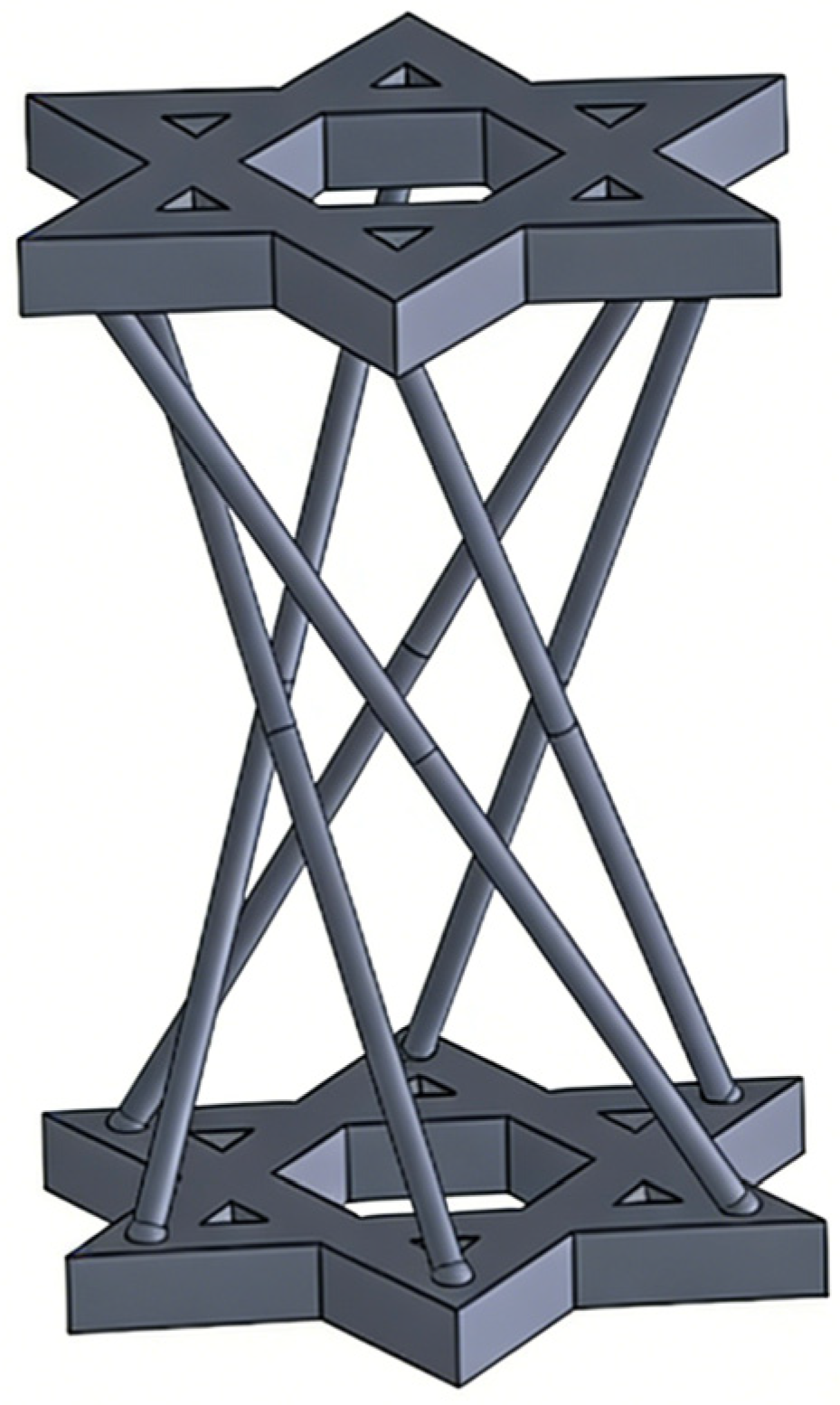
As illustrated in Figure 1, the object of study is an axisymmetric multi-rod parallel mechanism. The mechanism consists of two coaxial platforms (upper and lower) connected by multiple spatial spherical–rod–spherical linkages. The two ends of each rod are attached to spherical hinge points on the upper and lower platforms, respectively. These hinge points are uniformly distributed along the circumferences of the platforms, resulting in an overall configuration that exhibits rotational symmetry about the central axis.

During operation, the central axes of the two platforms remain coincident at all times. Their relative motion is characterized by an axial translation of the upper platform along the central axis, coupled with a relative rotation of the lower platform about the same axis. Owing to the constant lengths of all connecting rods, these two types of motion are not independent but are inherently coupled through the geometric constraints of the mechanism.

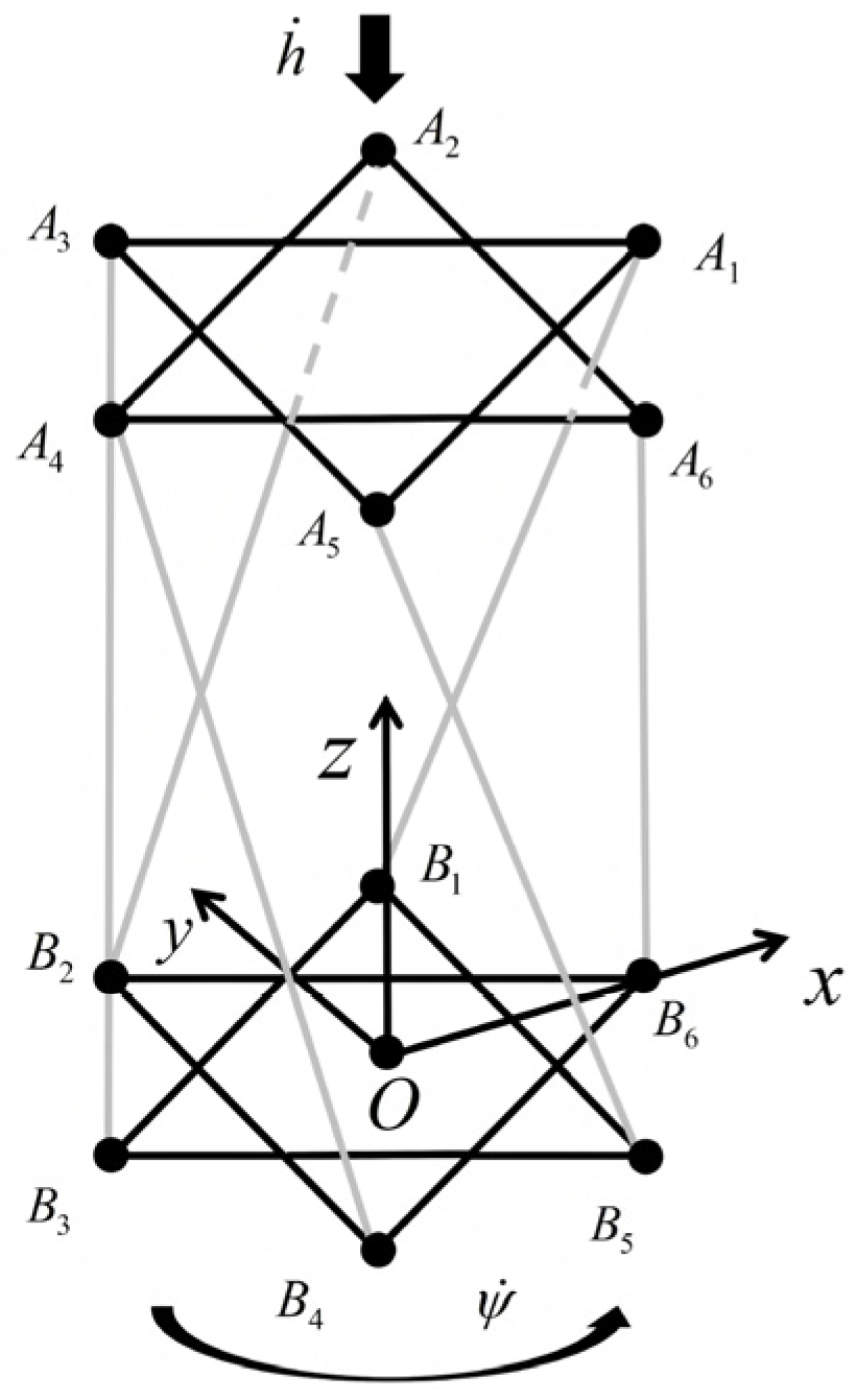
To describe the motion of the mechanism in a unified manner, a fixed coordinate system, Σ = {O, x, y, z}, is established, as shown in Figure 2. The center of the lower platform is taken as the origin O. The z-axis is defined along the common axis of symmetry of the upper and lower platforms and is directed upward. The x-axis is defined as the radial direction passing through hinge point A₁ of the upper platform when the lower platform is at the zero-rotation configuration, and the y-axis is determined according to the right-hand rule.

Within this coordinate system, the relative pose of the mechanism can be described by two generalized coordinates, namely, the axial height h and the relative rotation angle ψ. Accordingly, the generalized coordinate vector is defined as follows:

$$q=\left[\begin{array}{c}h\\ \psi \end{array}\right].$$

(1)

Here, h > 0 denotes the center-to-center distance of the upper platform relative to the lower platform along the z-axis, and ψ denotes the rotation angle of the lower platform relative to the upper platform about the z-axis. The z-axis coincides with the physical axis of symmetry of the mechanism. Accordingly, all quantities related to axial displacement, axial velocity, and variations in axial height in the following analysis are defined with respect to this physical axis.

Let the radii of the circles on which the hinge points of the upper and lower platforms are distributed be R_t and R_b, respectively. The mechanism consists of n spherical-rod-spherical linkages, and each platform is equipped with n spherical hinges uniformly distributed along its circumference. The circumferential angular position of the i-th hinge point is defined as follows:

$${\theta }_i={\theta }_0+{\displaystyle \frac{2\pi }{n}}(i-1),\hspace{1em}i=1,2,\dots ,n.$$

(2)

Here, θ₀ is the reference phase angle. For an ideal axisymmetric mechanism, the hinge points on the upper and lower platforms are topologically paired in a one-to-one correspondence according to the same index order. Accordingly, the position vectors of the connection points of the i-th rod on the upper and lower platforms can be expressed as

$$A_i(q)=\left[\begin{array}{c}{R}_t\cos {\theta }_i\\ R_t\sin {\theta }_i\\ h\end{array}\right],\hspace{1em}{B}_i(q)=\left[\begin{array}{c}{R}_b\cos ({\theta }_i+\psi )\\ R_b\sin ({\theta }_i+\psi )\\ 0\end{array}\right].$$

(3)

Therefore, the rod vector of the i-th rod is given by

$$d_i(q)=A_i(q)-B_i(q).$$

(4)

Its length is

$${\mathcal{l}}_i(q)=\Vert d_i(q){\Vert }_2.$$

(5)

Since the operating workspace satisfies h > 0, the z-component of the i-th rod vector, d_z,i(q) = h > 0, is always positive. Therefore, the z-components of all rod vectors have the same sign, which can be used to specify the vector orientation in the subsequent line-vector representation and thereby eliminate the sign ambiguity in line representation.

Substituting Equation (3) into Equations (4) and (5) yields

$${\mathcal{l}}^2(q)=h^2+R_t^2+R_b^2-2R_t{R}_b\cos \psi .$$

(6)

It follows from Equation (6) that, under the assumptions of ideal axisymmetric and uniform hinge distribution, ${\mathcal{l}}_i(q)$ is independent of the rod index i, that is, all n rods have the same length. Denoting this constant rod length by L, the feasible configurations of the mechanism must satisfy the constant-length constraint

$$F(h,\psi )\triangleq h^2+R_t^2+R_b^2-2R_t{R}_b\cos \psi -L^2=0.$$

(7)

From Equation (7), the analytical expression for the axial height as a function of the rotation angle can be directly obtained as

$$h(\psi )=\sqrt{L^2-R_t^2-R_b^2+2R_t{R}_b\cos \psi },\hspace{0.33em}\hspace{0.33em}\hspace{0.33em}h\ge 0.$$

(8)

To facilitate the description of the axial variation in the mechanism during rotation, the axial height variation relative to the zero configuration (ψ = 0) is further defined as

$$\Delta h(\psi )\triangleq L-h(\psi )=L-\sqrt{L^2-R_t^2-R_b^2+2R_t{R}_b\cos \psi }.$$

(9)

Equation (9) represents the downward displacement of the upper platform along the z-axis relative to the initial aligned configuration when the mechanism twists from the zero configuration to an angle ψ. Therefore, any scalar variation associated with the z-direction is, in essence, the change in the height of the upper platform along this physical axis.

Differentiating Equation (7) with respect to time yields the velocity-level constraint

$$h\dot{h}+R_t{R}_b\sin \psi \dot{\psi }=0.$$

(10)

Equation (10) indicates that, at any instantaneous configuration, the axial velocity $\dot{h}$ and the angular velocity $\dot{\psi }$ must satisfy a definite linear relation. In other words, although the instantaneous generalized velocity is formally written as $(\dot{h},\dot{\psi })$, it can vary only along the one-dimensional direction permitted by the constraint and cannot be specified independently. This property also provides the foundation for the subsequent construction of the feasible velocity direction, the mapping of characteristic velocities, and the inverse kinematic formulation.

Differentiating Equation (10) once more with respect to time gives the acceleration-level constraint

$${\dot{h}}^2+h\ddot{h}+R_t{R}_b\cos \psi {\dot{\psi }}^2+R_t{R}_b\sin \psi \ddot{\psi }=0.$$

(11)

When $\sin \psi =0$, one has

$$\psi =0\hspace{1em}\mathrm{or}\hspace{1em}\psi =\pi ,$$

(12)

Equation (10) degenerates into

$$h\dot{h}=0.$$

(13)

Since h > 0 always holds within the workspace, it follows that

$$\dot{h}=0.$$

(14)

This indicates that, under the above special configurations, the axial velocity component of the mechanism is instantaneously locked, that is, the platform cannot continue to extend or contract along the z-axis at that instant. These special configurations are referred to as dead-point configurations. However, the occurrence of a dead point here does not imply that the mechanism completely loses its mobility. Rather, it means that, at the velocity level, the admissible instantaneous motion direction degenerates: the axial component is constrained, whereas the rotational component about the z-axis may still exist. Meanwhile, at the acceleration level, the mechanism may still be able to move away from the dead-point configuration. Therefore, the dead point is better understood as a special property of the kinematic mapping, rather than as a complete loss of the mechanism’s degree of freedom in the geometric sense.

When the mechanism is fully axisymmetric, i.e., R_t = R_b, Equation (8) can be further simplified as

$$h(\psi )=\sqrt{L^2-2R^2+2R^2\cos \psi }.$$

(15)

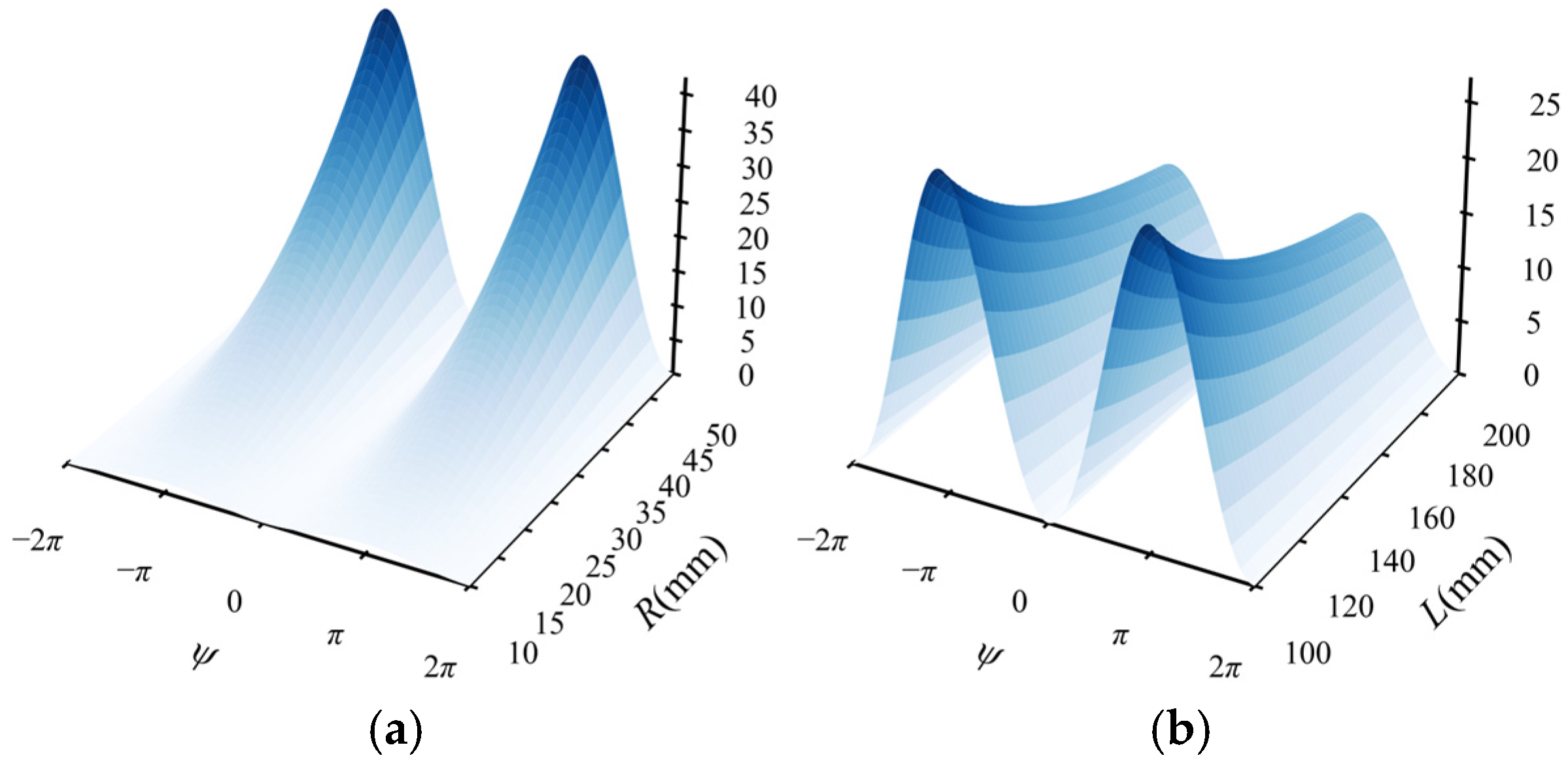
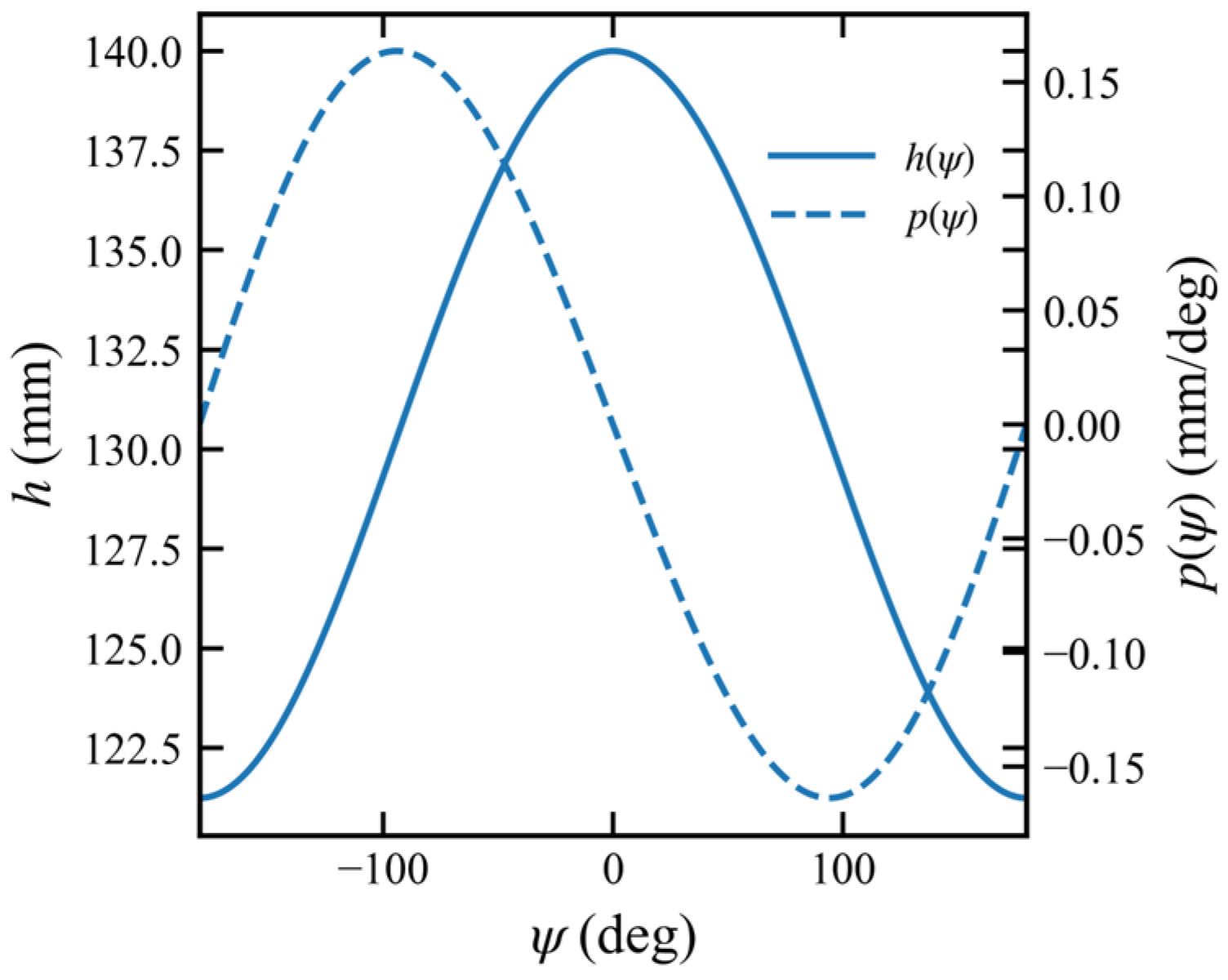
Furthermore, Equation (9) gives the relationship between the axial height variation and the configuration, as illustrated in Figure 3.

As shown in Figure 3, the rotation angle ψ is taken over the interval [−2π,2π], while the hinge-distribution radius R and the rod length L are varied separately. It can be observed that Δh(ψ) exhibits two periods within [−2π,2π], with a fundamental period of 2π. As ψ increases from 0 to π, Δh increases monotonically; as ψ further increases from π to 2π, Δh returns to a smaller value, thereby forming a symmetric return branch. That is,

$$\Delta h(\psi )=\Delta h(\psi +2k\pi ),\hspace{1em}\Delta h(\psi )=\Delta h(2\pi -\psi ),$$

(16)

where $k\in \mathbb{Z}$.

Therefore, without loss of generality, it is sufficient to consider the principal interval

$$\psi \in [0,\pi ],$$

(17)

This angular interval covers all non-redundant configurations from the zero configuration to a half-turn rotation and thus serves as the basic domain for the subsequent numerical analysis.

To transition from the discrete rod geometry to the subsequent continuous line-field representation, the circumferential hinge angle is further continued by letting θ ∈ [0,2π), and the generatrix parameter t ∈ [0,1] is introduced. Accordingly, a continuous generatrix corresponding to the circumferential position θ can be expressed as

$$P(\theta ,t)=B(\theta ,q)+t\left(A(\theta ,q)-B(\theta ,q)\right),$$

(18)

where

$$A(\theta ,q)=\left[\begin{array}{c}{R}_t\cos \theta \\ R_t\sin \theta \\ h\end{array}\right],\hspace{1em}B(\theta ,q)=\left[\begin{array}{c}{R}_b\cos (\theta +\psi )\\ R_b\sin (\theta +\psi )\\ 0\end{array}\right].$$

(19)

Equation (18) shows that the parameter t performs a linear interpolation between the lower-platform hinge point B(θ,q) and the upper-platform hinge point A(θ,q), and therefore specifies an arbitrary point on the corresponding generatrix. Since the z-coordinates of the upper and lower hinge points are h and 0, respectively, any point on the generatrix satisfies

$$z=th.$$

(20)

Projecting Equation (18) onto the xy-plane and considering the cross-sectional radial coordinate under the condition of complete axisymmetric R_t = R_b, one obtains

$$\rho (t,\psi )=(1-t)R{e}^{i\psi }+tR.$$

(21)

Further, by letting

$$t={\displaystyle \frac{z}{h}},\hspace{1em}\zeta =z-{\displaystyle \frac{h}{2}},$$

(22)

the envelope surface generated by this family of generatrices can be transformed into the standard quadric form

$${\displaystyle \frac{x^2+y^2}{{\left(R\cos (\psi /2)\right)}^2}}-{\displaystyle \frac{{\left(z-h/2\right)}^2}{{\left(h/(2\tan (\psi /2))\right)}^2}}=1,\hspace{1em}\psi \in (0,\pi ).$$

(23)

Equation (23) indicates that, under ideal axisymmetric and non-degenerate configurations, the continuous extension of the rod axes generates a ruled surface symmetric about the z-axis, whose typical form is a one-sheeted hyperboloid. This shows that the multiple rod axes in the mechanism under study are not merely a set of discrete spatial lines, but collectively form a rod-axis envelope surface with a well-defined analytical structure.

From Equation (23), the waist radius of this surface can also be obtained as

$${\rho }_w(\psi )=R\cos {\displaystyle \frac{\psi }{2}}.$$

(24)

It follows that the rotation angle ψ directly determines the geometric form of the enveloping hyperboloid. ψ → 0,

$$\cos {\displaystyle \frac{\psi }{2}}\to 1,\hspace{1em}\tan {\displaystyle \frac{\psi }{2}}\to 0,$$

(25)

In this limit, the axial semi-axis of the surface tends to infinity, and the limiting form approaches a cylindrical surface of radius R. By contrast, as ψ → π⁻,

$${\rho }_w(\psi )\to 0,$$

(26)

the surface gradually contracts, the waist disappears, and the geometry tends toward a degenerate intersecting configuration.

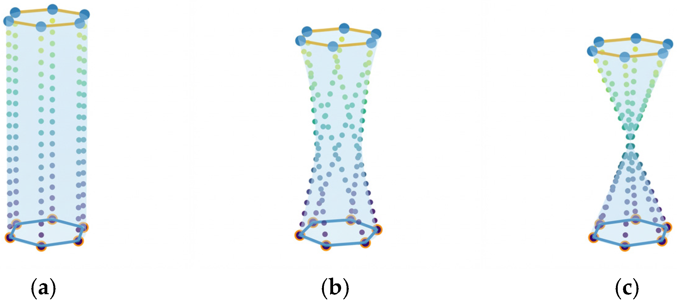
As shown in Figure 4, as the relative rotation angle ψ of the two platforms gradually increases from a small value, the rod-axis envelope surface undergoes a continuous evolution from a “near-cylindrical form” to a “one-sheeted hyperboloid”, and finally to a “degenerate intersecting form”. Figure 4a corresponds to the small-angle case, in which the generatrices are nearly parallel and the overall geometry approaches a cylindrical surface; Figure 4b corresponds to an intermediate rotation angle, where the generatrices exhibit the typical waist-contraction feature of a hyperboloid; and Figure 4c corresponds to the case where ψ approaches π, in which the waist radius tends to zero and the generatrices gradually converge toward the center. This figure provides an intuitive geometric illustration of the variation law of the envelope surface revealed by Equations (23) and (24).

This result indicates that, under the axisymmetric assumption, the discrete rod axes can be naturally elevated to a family of spatial straight lines varying continuously along the circumferential direction. Therefore, the overall geometric state of the mechanism can be described not only by the discrete set of individual rods, but also in a unified manner through a continuous rod-axis field.

2.2. Plücker Line Field and Envelope Feature Vector

At a given configuration q, the six rod axes of the mechanism shown in Figure 1 constitute a set of oriented spatial lines. To simultaneously describe the direction of each rod axis and its spatial position relative to the coordinate origin, Plücker coordinates are adopted as a unified representation of the rod axes. The Plücker representation is a classical homogeneous representation of spatial lines and has been widely used in line geometry, screw theory, mechanism science, and robot geometric modeling [24,25,26,27]. From an engineering perspective, its advantage lies in the fact that it avoids repeatedly switching among different points on the same line. Instead, the entire oriented line can be encoded as a six-dimensional quantity using only one direction vector and one moment vector with respect to the origin, which facilitates the unified treatment of the complete set of rod axes.

For the i-th rod, let a point on its axis be the lower-platform hinge point B_i(q), and let the direction vector be the rod vector d_i(q) defined in Equation (4). The corresponding primitive Plücker line vector is then defined as

$${\tilde{L}}_i(q)=\left[\begin{array}{c}{d}_i(q)\\ m_i(q)\end{array}\right]\in {ℝ}^6,\hspace{1em}{m}_i(q)=B_i(q)\times d_i(q).$$

(27)

Expanding it into six scalar components gives

$${\tilde{L}}_i(q)={\left[\begin{array}{cccccc}{d}_{x,i}& d_{y,i}& d_{z,i}& m_{x,i}& m_{y,i}& m_{z,i}\end{array}\right]}^{⊺}.$$

(28)

Here, the first three components $(d_{x,i},d_{y,i},d_{z,i})$ describe the direction of the rod axis, whereas the last three components $(m_{x,i},m_{y,i},m_{z,i})$ describe the moment offset of the line relative to the origin. Therefore, the Plücker line vector provides a unified geometric description that combines the rod-axis orientation and its spatial offset.

The Plücker representation is essentially homogeneous: the same oriented line can be represented by any nonzero scalar multiple of ${[d_i^{⊺},m_i^{⊺}]}^{⊺}$, ${[d_i^{⊺},m_i^{⊺}]}^{⊺}~{[-d_i^{⊺},-m_i^{⊺}]}^{⊺}$.

To fix this sign freedom throughout the workspace, this study consistently adopts the orientation convention from the lower platform toward the upper platform, namely,

$$d_i(q)=A_i(q)-B_i(q),\hspace{1em}{d}_{z,i}(q)=h>0.$$

(29)

Since h > 0 holds throughout the workspace, the z-components of all rod axes remain positive. Consequently, the sign convention for the line direction can be maintained consistently over the entire workspace.

To eliminate the arbitrary scale introduced by the magnitude of the direction vector in the Plücker representation and to facilitate coefficient comparison among different configurations, Equation (27) is further normalized by the rod length ${\mathcal{l}}_i(q)$. Define

$$d_i^{*}(q)={\displaystyle \frac{d_i(q)}{{\mathcal{l}}_i(q)}},\hspace{1em}{m}_i^{*}(q)={\displaystyle \frac{m_i(q)}{{\mathcal{l}}_i(q)}},\hspace{1em}{L}_i(q)=\left[\begin{array}{c}{d}_i^{*}(q)\\ m_i^{*}(q)\end{array}\right].$$

(30)

Here, $d_i^{*}$ is dimensionless, whereas $m_i^{*}$ retains the dimension of length. The vector L_i(q) obtained from Equation (30) serves as the basic object for the subsequent modeling of both the discrete line field and the continuous line field. For simplicity of notation, the six normalized components are still denoted by d_x, d_y, d_z, m_x, m_y, m_z.

By stacking the normalized Plücker line vectors of all n rods row by row, the discrete line-set matrix is obtained as

$$Y(q)=\left[\begin{array}{c}{L}_1^{⊺}(q)\\ L_2^{⊺}(q)\\ ⋮\\ L_n^{⊺}(q)\end{array}\right]\in {ℝ}^{n\times 6}.$$

(31)

Each row of Y(q) corresponds to the six-dimensional geometric description of one rod axis, and each column corresponds to one of the six components d_x, d_y, d_z, m_x, m_y, m_z. Therefore, Y(q) can be regarded as the sampling matrix of the current discrete rod-axis field of the mechanism.

Because the rods are uniformly distributed along the circumferential direction, the mechanism geometry is naturally periodic with respect to the circumferential angle. The most natural continuous variable is therefore the circumferential angle $\theta \in [0,2\pi )$. Accordingly, a truncated Fourier basis is adopted to construct a circumferentially continuous representation of the discrete line field. The basis function vector truncated at order N_h is defined as

$$\varphi (\theta )=\left[\begin{array}{cccccc}1\hfill & \cos \theta & \sin \theta & \cdots & \cos (N_h\theta )& \hfill \sin (N_h\theta )\end{array}\right],$$

(32)

and the basis matrix corresponding to the discrete samples ${\left\{{\theta }_i\right\}}_{i=1}^n$ is constructed as

$$\Phi =\left[\begin{array}{c}\varphi ({\theta }_1)\\ \varphi ({\theta }_2)\\ ⋮\\ \varphi ({\theta }_n)\end{array}\right]\in {ℝ}^{n\times (2N_h+1)}.$$

(33)

Hence, the discrete line-set matrix Y(q) can be written as

$$Y(q)=\Phi C(q),\hspace{1em}C(q)\in {ℝ}^{(2N_h+1)\times 6}.$$

(34)

Here, C(q) is the Fourier coefficient matrix of the line field. Its columns correspond one-to-one with the six Plücker components, namely,

$$C(q)=\left[\begin{array}{c}{c}_{d_x}(q),c_{d_y}(q),c_{d_z}(q),c_{m_x}(q),c_{m_y}(q),c_{m_z}(q)\end{array}\right].$$

(35)

This means that each Plücker component is represented as a spectral expansion with respect to the circumferential angle θ whereas C(q) summarizes the circumferential geometric pattern of the entire rod-axis set. Compared with treating the six rods individually, this representation transforms the “discrete rod set” into a “continuous line field”, thereby compressing the overall geometric state of the mechanism into a low-dimensional and structured coefficient matrix.

When n ≥ 2N_h + 1 and the sampling-angle set is nondegenerate, C(q) is uniquely determined in the least-squares sense by

$$C(q)={\Phi }^{+}Y(q),\hspace{1em}{\Phi }^{+}={\left({\Phi }^{⊺}\Phi \right)}^{-1}{\Phi }^{⊺}.$$

(36)

For the uniform sampling adopted in this study, ${\theta }_i={\theta }_0+{\displaystyle \frac{2\pi }{n}}(i-1)$, the matrix ${\Phi }^{⊺}\Phi$ has a strict diagonal structure and can be written as

$${\Phi }^{⊺}\Phi =\mathrm{diag}\left(n,{\displaystyle \frac{n}{2}},{\displaystyle \frac{n}{2}},\dots ,{\displaystyle \frac{n}{2}}\right).$$

(37)

Therefore, its pseudoinverse can be further simplified as

$${\Phi }^{+}=\mathrm{diag}\left({\displaystyle \frac{1}{n}},{\displaystyle \frac{2}{n}},{\displaystyle \frac{2}{n}},\dots ,{\displaystyle \frac{2}{n}}\right){\Phi }^{⊺}.$$

(38)

Equations (34)–(38) show that the discrete rod-axis set matrix Y(q) is analytically projected onto the low-order spectral coefficient matrix C(q). For a general mechanism, this representation is a low-order approximation. However, for the ideal axisymmetric mechanism considered in the remainder of this paper, the next subsection will further show that, when N_h = 1, this representation reduces to an exact closed-form result.

When N_h = 1, the coefficient matrix C(q) consists of a constant term, a first-order cosine term, and a first-order sine term, and can be written as

$$C(q)=\left[\begin{array}{c}{c}_0^{⊺}(q)\\ {(c_1^c(q))}^{⊺}\\ {(c_1^s(q))}^{⊺}\end{array}\right],\hspace{1em}{c}_0,c_1^c,c_1^s\in {ℝ}^6.$$

(39)

Accordingly, the feature vector is defined as

$$f(q)=\mathrm{vec}\left(C(q)\right)\in {ℝ}^{6(2N_h+1)}.$$

(40)

When N_h = 1, one has

$$f(q)=\left[\begin{array}{c}{c}_0(q)\\ c_1^c(q)\\ c_1^s(q)\end{array}\right]\in {ℝ}^{18}.$$

(41)

From an engineering perspective, f(q) serves as a low-dimensional “fingerprint” of the geometric state of the entire rod-axis assembly. Specifically, c₀ describes the overall line-field structure in the circumferentially averaged sense, whereas $c_1^c$ and $c_1^s$ characterize the dominant first-order modes of the circumferential variation in the rod-axis distribution. In other words, f(q) compactly encapsulates how the six rods are arranged as a whole and how this arrangement varies, thereby providing an interpretable feature space for the subsequent construction of velocity mappings, sensitivity analysis, and inverse kinematics.

According to Equation (34), for an arbitrary circumferential angle θ, the Plücker representation of the continuous line field at that position can be written as

$$L^{⊺}(\theta ;q)=\varphi (\theta )C(q).$$

(42)

Differentiating with respect to time yields the instantaneous rate of change in the continuous line field,

$${\dot{L}}^{⊺}(\theta ;q)=\varphi (\theta )\dot{C}(q)=\varphi (\theta ){\displaystyle \frac{\partial C(q)}{\partial q}}\dot{q}.$$

(43)

Correspondingly, in the feature space,

$$\dot{f}(q)=J_f(q)\dot{q},\hspace{0.33em}\hspace{0.33em}\hspace{0.33em}{J}_f(q)={\displaystyle \frac{\partial f(q)}{\partial q}}\in {ℝ}^{6(2N_h+1)\times 2}.$$

(44)

Equation (44) gives the analytical mapping from the generalized velocity $\dot{q}$ to the feature velocity $\dot{f}$.

2.3. Closed-Form Characteristic Coefficients Under Axisymmetry

Under the assumptions of ideal axisymmetric and uniform circumferential distribution of hinge points, the continuous angular parameter θ can be used directly to derive a closed-form expression for the line-field coefficient matrix C(q). For notational simplicity, the following intermediate variables are introduced:

$$s=\sin \psi ,\hspace{0.33em}\hspace{0.33em}\hspace{0.33em}c=\cos \psi ,\hspace{0.33em}\hspace{0.33em}\hspace{0.33em}k=R_t{R}_b,\hspace{0.33em}\hspace{0.33em}\hspace{0.33em}a=R_t-R_{b}c,\hspace{0.33em}\hspace{0.33em}\hspace{0.33em}b=R_{b}s,$$

(45)

and

$$\mathcal{l}=\sqrt{h^2+R_t^2+R_b^2-2kc},\hspace{0.33em}\hspace{0.33em}\hspace{0.33em}\iota ={\displaystyle \frac{1}{\mathcal{l}}}.$$

(46)

Here, $\mathcal{l}$ is the common length of an arbitrary rod, and ι is its reciprocal. From Equations (3) and (4), the continuous rod vector is obtained as

$$d(\theta ;q)=A(\theta ,q)-B(\theta ,q),$$

(47)

whose three components can be expanded as

$$d_x(\theta )=a\cos \theta +b\sin \theta ,\hspace{0.33em}\hspace{0.33em}\hspace{0.33em}{d}_y(\theta )=a\sin \theta -b\cos \theta ,\hspace{0.33em}\hspace{0.33em}\hspace{0.33em}{d}_z(\theta )=h.$$

(48)

Correspondingly, from

$$m(\theta ;q)=B(\theta ,q)\times d(\theta ;q),$$

(49)

the moment components are obtained as

$$m_x(\theta )=h{R}_b\sin (\theta +\psi ),\hspace{0.33em}\hspace{0.33em}\hspace{0.33em}{m}_y(\theta )=-h{R}_b\cos (\theta +\psi ),\hspace{0.33em}\hspace{0.33em}\hspace{0.33em}{m}_z(\theta )=-R_t{R}_b\sin \psi =-ks.$$

(50)

Hence, the normalized Plücker line field is

$$L(\theta ;q)=\left[\begin{array}{c}{d}^{*}(\theta ;q)\\ m^{*}(\theta ;q)\end{array}\right]=\left[\begin{array}{c}\iota d(\theta ;q)\\ \iota m(\theta ;q)\end{array}\right],$$

(51)

and its components can be rearranged as

$$d_x^{*}(\theta )=a\iota \cos \theta +b\iota \sin \theta ,$$

(52)

$$d_y^{*}(\theta )=-b\iota \cos \theta +a\iota \sin \theta ,$$

(53)

$$d_z^{*}(\theta )=h\iota ,$$

(54)

$$m_x^{*}(\theta )=hb\iota \cos \theta +h{R}_{b}c\iota \sin \theta ,$$

(55)

$$m_y^{*}(\theta )=-h{R}_{b}c\iota \cos \theta +hb\iota \sin \theta ,$$

(56)

$$m_z^{*}(\theta )=-ks\iota .$$

(57)

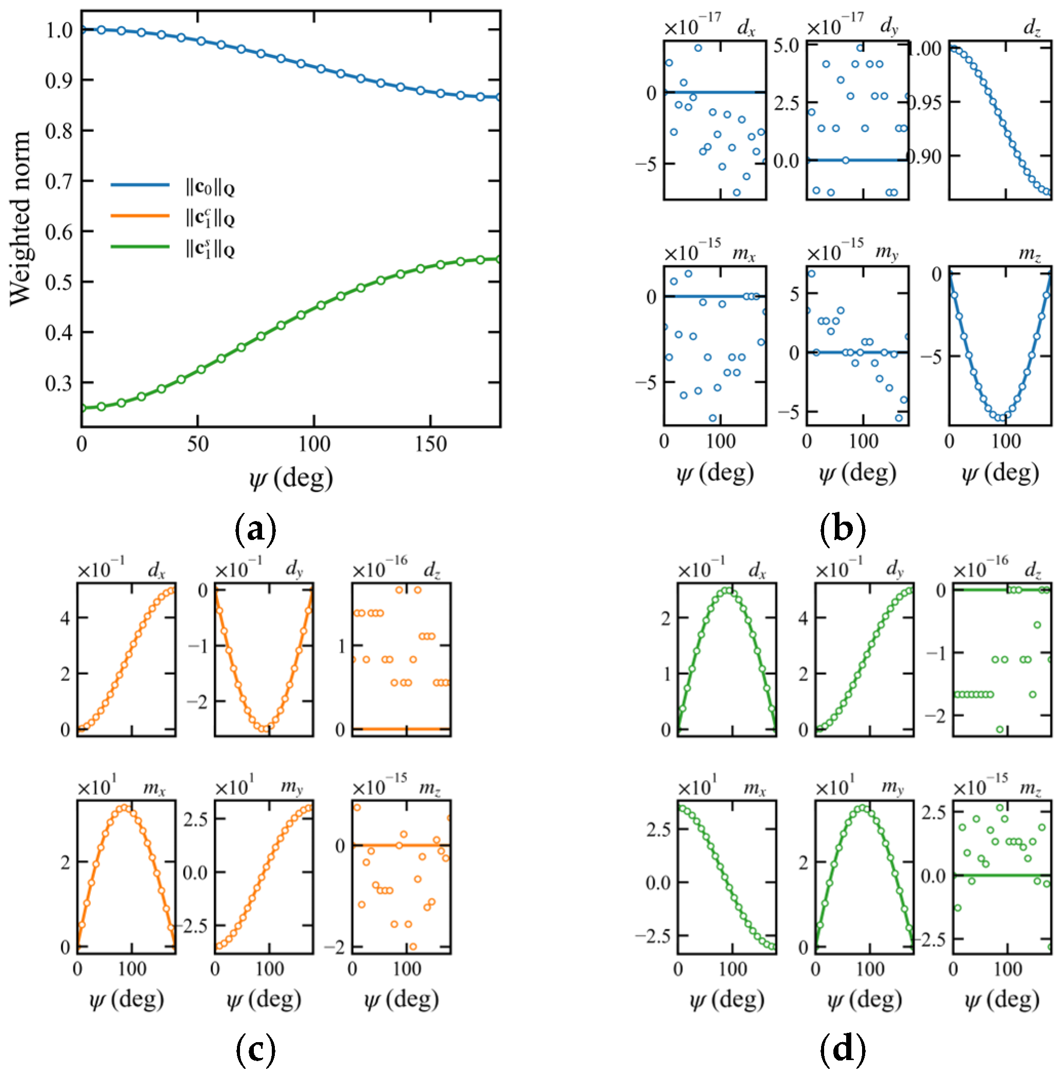
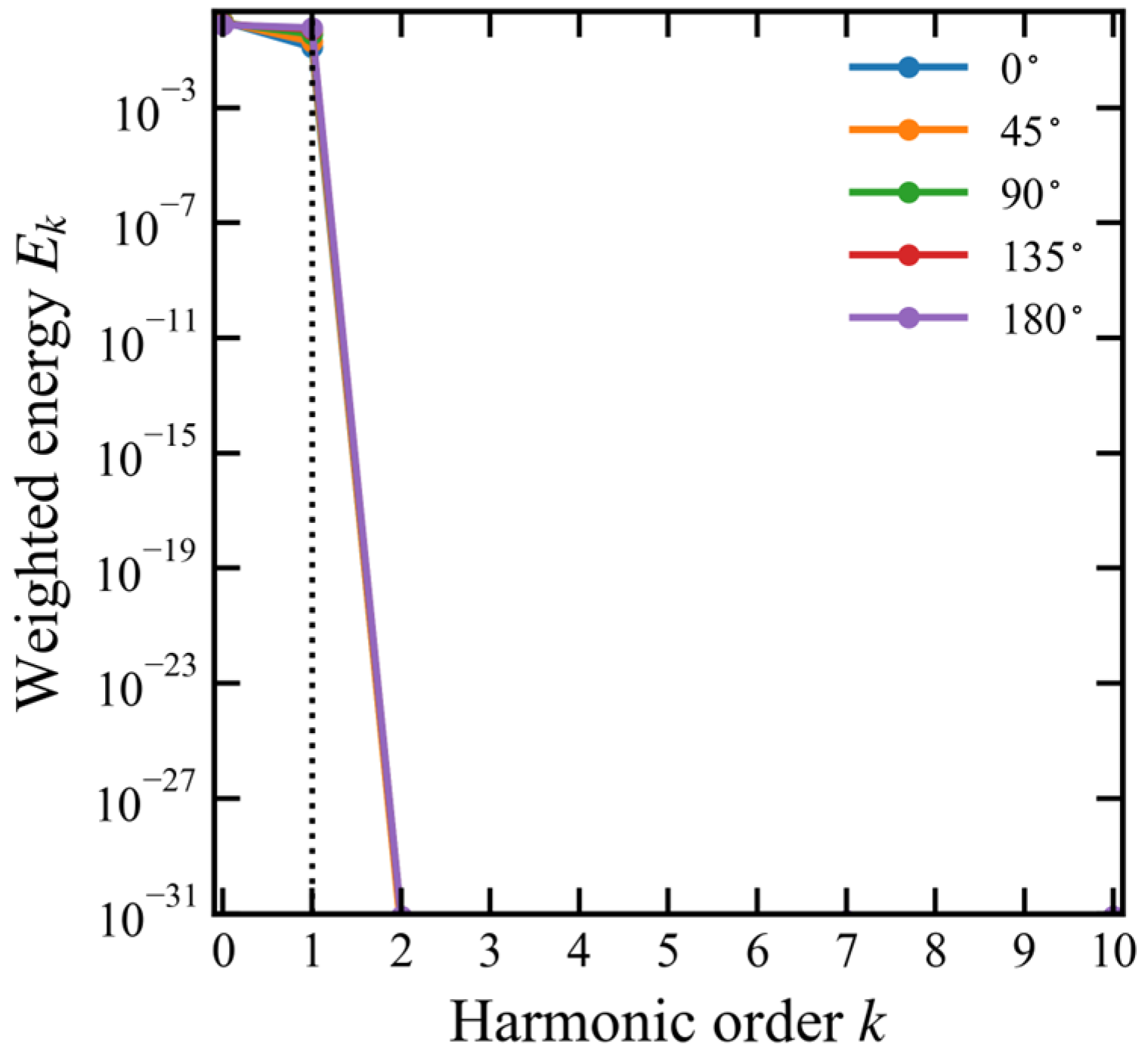
It can be seen from Equations (52)–(57) that, except for the constant terms, all θ-dependent components contain only the first-order harmonics $\{\cos \theta ,\sin \theta \}$, with no second- or higher-order harmonic terms. Therefore, for the ideal axisymmetric model, when the truncation order is chosen as N_h = 1, the Fourier representation in Equation (34) is an exact analytical expansion. That is, under this ideal condition, Y(q) = ΦC(q) is an exact identity.

For notational uniformity, let an arbitrary normalized line-field component x(θ) be written as

$$x(\theta )=c_0+c_1^c\cos \theta +c_1^s\sin \theta .$$

(58)

Accordingly, the constant term, the first-order cosine term, and the first-order sine term of each component can be directly identified, yielding the closed-form coefficient matrix for N_h = 1

$$C(q)=\left[\begin{array}{cccccc}{c}_0^{d_x}& c_0^{d_y}& c_0^{d_z}& c_0^{m_x}& c_0^{m_y}& c_0^{m_z}\\ c_1^{d_x,c}& c_1^{d_y,c}& c_1^{d_z,c}& c_1^{m_x,c}& c_1^{m_y,c}& c_1^{m_z,c}\\ c_1^{d_x,s}& c_1^{d_y,s}& c_1^{d_z,s}& c_1^{m_x,s}& c_1^{m_y,s}& c_1^{m_z,s}\end{array}\right]=\left[\begin{array}{cccccc}0& 0& hu& 0& 0& -ksu\\ a\iota & -b\iota & 0& hb\iota & -h{R}_{b}c\iota & 0\\ b\iota & a\iota & 0& h{R}_{b}c\iota & hb\iota & 0\end{array}\right],$$

(59)

Here, the six columns correspond to (d_x, d_y, d_z, m_x, m_y, m_z), respectively, whereas the three rows correspond to the coefficients $(c_0,c_1^c,c_1^s)$ associated with each Plücker component.

As can be seen from Equation (59), under ideal axisymmetric, the entire continuous rod-axis field is completely determined by only 18 closed-form characteristic coefficients, without the need to introduce higher-order harmonic terms. This result has two important implications. First, it shows that the feature vector $f(q)=\mathrm{vec}(C(q))\in {ℝ}^{18}$ constructed in this study is a rigorously consistent low-dimensional analytical representation of the ideal axisymmetric geometry. Second, it implies that the subsequent feature Jacobian J_f(q) can be obtained directly by differentiating Equation (59), thereby laying the foundation for the analytical inverse mappings at both the velocity and acceleration levels.

From an engineering viewpoint, Equations (58) and (59) show that, for an ideal axisymmetric mechanism, the circumferential geometric distribution of the entire rod-axis set does not need to be treated rod by rod. Instead, it can be completely characterized by a “constant block and first-order cosine block and first-order sine block”. For this reason, what must actually be tracked in the subsequent inverse analysis is not each individual rod axis itself, but rather the evolution of these 18 analytical characteristic coefficients with the configuration (h,ψ).

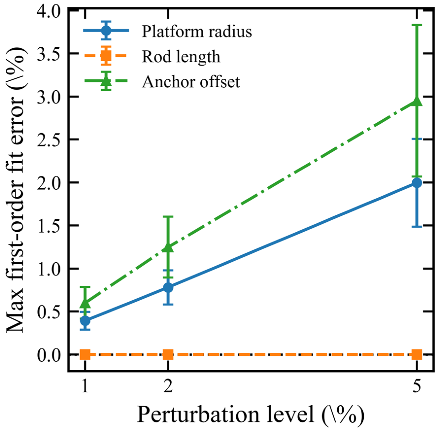
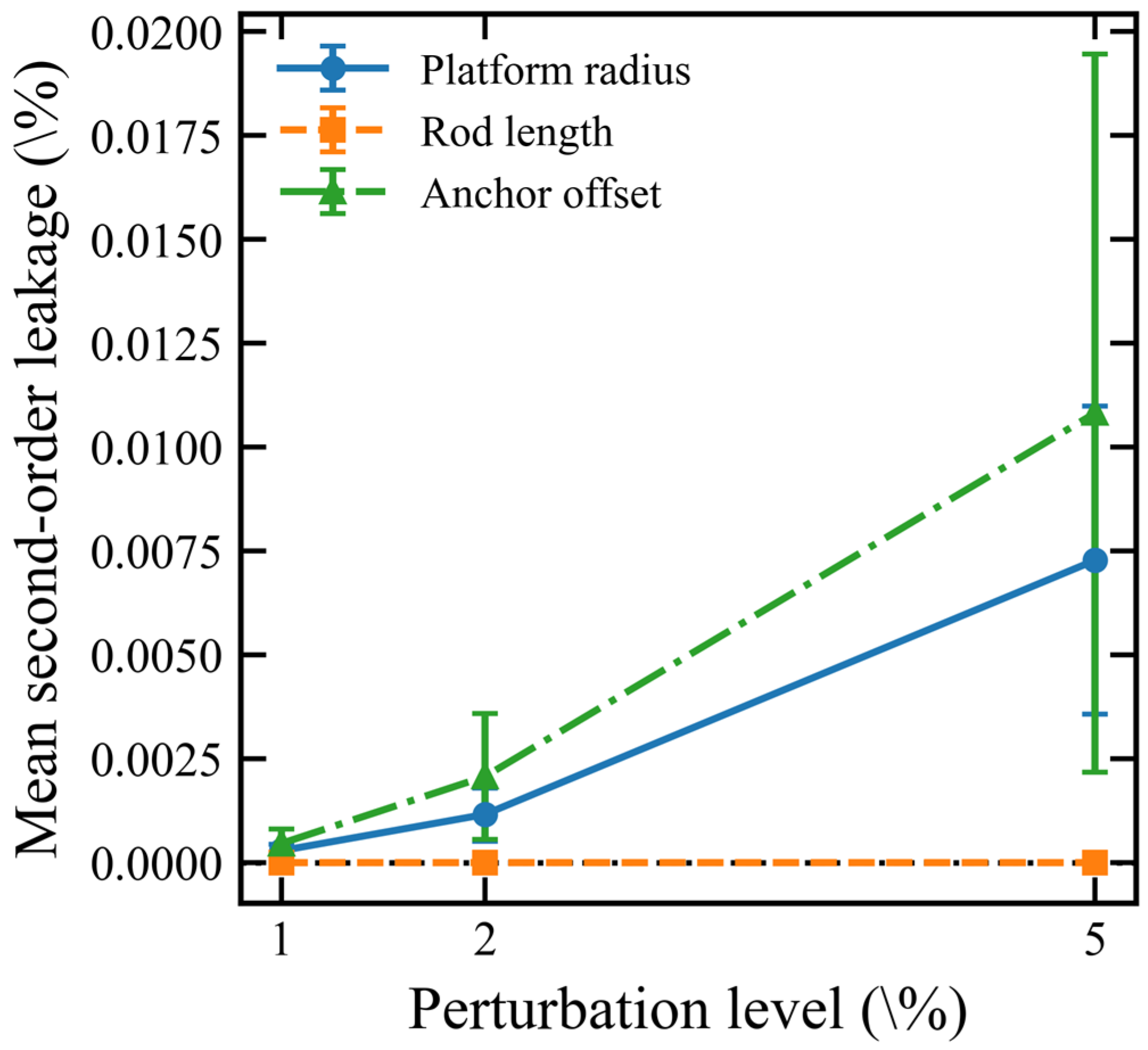
The above first-order exact representation is established under the assumptions of ideal axisymmetric and uniform hinge distribution. If symmetry-breaking factors are present, such as assembly errors, hinge-angle deviations, or inconsistent radii, the second- and higher-order harmonics generally no longer vanish identically. In that case, N_h = 1 degenerates from a “strictly exact representation” to a dominant low-order approximation.

2.4. Feature Kinematics and a Dead-Point-Stable Inverse Framework

2.4.1. Feature Representation of the Line-Field Twist and Analytical Feature Jacobian

As established above, the line-field feature vector of the mechanism at configuration q is defined as f(q) = vec(C(q)), where C(q) is the closed-form characteristic coefficient matrix under first-order truncation. Accordingly, when the mechanism configuration q(t) varies with time, the time derivative of f(q(t)) is naturally defined as the feature velocity:

$$\dot{f}={\displaystyle \frac{\mathrm{d}}{\mathrm{d}t}}f(q(t)).$$

(60)

From an engineering perspective, $\dot{f}$ describes the instantaneous rate of change, in the feature coordinate system, of the continuous line field formed by the entire set of rod axes, rather than the local variation in any single rod. Therefore, it can be regarded as the “motion velocity” of the overall geometric state of the mechanism in feature space.

Applying the chain rule to f(q) yields the linear mapping between the feature velocity and the generalized velocity $\dot{q}={[\dot{h},\dot{\psi }]}^{⊺}$:

$$\begin{array}{cc}\dot{f}=J_f(q)\dot{q},& \hspace{0.33em}\hspace{0.33em}\hspace{0.33em}{J}_f(q)\triangleq {\displaystyle \frac{\partial f(q)}{\partial q}}=\left[\begin{array}{cc}{\displaystyle \frac{\partial f}{\partial h}}& {\displaystyle \frac{\partial f}{\partial \psi }}\end{array}\right].\end{array}$$

(61)

When the truncation order is N_h = 1, one has $C(q)\in {ℝ}^{3\times 6}$, $f(q)\in {ℝ}^{18}$, and $J_f(q)\in {ℝ}^{18\times 2}$. Since f(q) = vec(C(q)), Equation (61) can be further rewritten as

$$J_f(q)=\left[\mathrm{vec}\left({\displaystyle \frac{\partial C}{\partial h}}\right)\hspace{0.33em}\hspace{0.33em}\hspace{0.33em}\mathrm{vec}\left({\displaystyle \frac{\partial C}{\partial \psi }}\right)\right]=\left[\begin{array}{cc}\mathrm{vec}(C_h)& \mathrm{vec}(C_{\psi })\end{array}\right],$$

(62)

where

$$C_h={\displaystyle \frac{\partial C}{\partial h}},\hspace{0.33em}\hspace{0.33em}\hspace{0.33em}{C}_{\psi }={\displaystyle \frac{\partial C}{\partial \psi }}.$$

(63)

Therefore, the analytical feature Jacobian can be obtained simply by differentiating the closed-form coefficient matrix C(q) derived in the previous subsection with respect to h and ψ.

Using the preceding notation and evaluating the required derivatives gives

$${\displaystyle \frac{\partial a}{\partial h}}=0,\hspace{0.33em}\hspace{0.33em}\hspace{0.33em}{\displaystyle \frac{\partial b}{\partial h}}=0,\hspace{0.33em}\hspace{0.33em}\hspace{0.33em}{\displaystyle \frac{\partial \iota }{\partial h}}=-h{\iota }^3,\hspace{0.33em}\hspace{0.33em}\hspace{0.33em}{\displaystyle \frac{\partial a}{\partial \psi }}=b,\hspace{0.33em}\hspace{0.33em}\hspace{0.33em}{\displaystyle \frac{\partial b}{\partial \psi }}=R_{b}c,\hspace{0.33em}\hspace{0.33em}\hspace{0.33em}{\displaystyle \frac{\partial \iota }{\partial \psi }}=-ks{\iota }^3.$$

(64)

Based on the closed-form coefficient matrix for the axisymmetric case with N_h = 1, term-by-term differentiation with respect to h and ψ yields C_h and C_ψ. From Equation (59), one obtains

$$C_h=\left[\begin{array}{cccccc}0& 0& \iota -h^2{\iota }^3& 0& 0& khs{\iota }^3\\ -ah{\iota }^3& bh{\iota }^3& 0& b\iota -h^{2}b{\iota }^3& -R_{b}c\iota +h^2{R}_{b}c{\iota }^3& 0\\ -bh{\iota }^3& -ah{\iota }^3& 0& R_{b}c\iota -h^2{R}_{b}c{\iota }^3& b\iota -h^{2}b{\iota }^3& 0\end{array}\right],$$

(65)

and

$$C_{\psi }=\left[\begin{array}{cccccc}0& 0& -hks{\iota }^3& 0& 0& -kc\iota +k^2{s}^2{\iota }^3\\ b\iota -aks{\iota }^3& -R_{b}c\iota +bks{\iota }^3& 0& h{R}_{b}c\iota -hbks{\iota }^3& hb\iota +h{R}_{b}cks{\iota }^3& 0\\ R_{b}c\iota -bks{\iota }^3& b\iota -aks{\iota }^3& 0& -hb\iota -h{R}_{b}cks{\iota }^3& h{R}_{b}c\iota -hbks{\iota }^3& 0\end{array}\right].$$

(66)

Since $\dot{f}$ depends linearly on $\dot{q}$, setting $\dot{q}={[1,0]}^{⊺}$ yields $\mathrm{vec}(C_h)$, whereas setting $\dot{q}={[0,1]}^{⊺}$ yields $\mathrm{vec}(C_{\psi })$, in full agreement with the analytical derivatives.

Equations (62)–(66) provide the complete analytical form of the feature Jacobian J_f(q). Its significance lies in the following: once the axial–twisting generalized velocity $\dot{q}$ of the platform is specified, the instantaneous variation $\dot{f}$ of the continuous Plücker line field in feature space can be computed directly through J_f(q). Compared with conventional approaches that construct the Jacobian rod by rod from discrete linkages, the present formulation yields an analytical mapping for the global line-field features, with fixed dimension, clear structure, and explicit geometric interpretability.

2.4.2. Velocity Constraint, Dead Points, and the Origin of Invertibility

From Equation (10), the mechanism satisfies the constant-length constraint at the velocity level:

$$h\dot{h}+k\sin \psi \dot{\psi }=0.$$

(67)

Writing this in vector form gives

$$a{(q)}^{⊺}\dot{q}=0,\hspace{0.33em}\hspace{0.33em}\hspace{0.33em}a(q)=\left[\begin{array}{c}h\\ k\sin \psi \end{array}\right].$$

(68)

Equation (68) indicates that, although the generalized velocity is formally written as $\dot{q}={[\dot{h},\dot{\psi }]}^{⊺}$, its two components cannot be prescribed independently. Instead, they must lie in the one-dimensional feasible subspace defined by the constraint. That is, at any configuration, the mechanism possesses only one admissible velocity direction. This also forms the basis for the subsequent analysis of feasible directions, feasible sensitivity, and worst-case amplification.

When

$$\sin \psi =0,\hspace{0.33em}\hspace{0.33em}\hspace{0.33em}\psi =0,\pm \pi ,\pm 2\pi ,\dots ,$$

(69)

the mechanism is at a dead point. Since h > 0 always holds within the workspace, Equation (69) degenerates to

$$h\dot{h}=0 \Rightarrow \dot{h}=0.$$

(70)

This indicates that, at a dead point, the axial velocity component of the mechanism is instantaneously locked, and the admissible motion can only develop along a direction dominated by $\dot{\psi }$. It should be emphasized that this “locking” occurs only at the velocity level; it neither implies that the mechanism has completely lost its mobility nor means that the feature mapping automatically fails at that point.

To clarify this point, consider a representative feature component, namely the coefficient of the m_z component in the constant block. From Equation (59), one has

$$c_0^{m_z}(q)=-ks\iota .$$

(71)

Differentiating it with respect to ψ gives

$${\displaystyle \frac{\partial c_0^{m_z}}{\partial \psi }}=-kc\iota +k^2{s}^2{\iota }^3.$$

(72)

At the dead point where $\sin \psi =0$, this expression further simplifies to

$${\left.{\displaystyle \frac{\partial c_0^{m_z}}{\partial \psi }}\right|}_{\psi =0,\pm \pi }=-kc\iota \ne 0.$$

(73)

Equation (73) shows that even at a dead point, the first-order response of the line-field features to the rotation angle ψ remains nonzero. In other words, a dead point does not mean that the feature space ceases to vary; rather, it means only that, under the velocity constraint, the feasible direction of the generalized velocity degenerates. It follows that the difficulty of inverse mapping near a dead point does not arise from a complete loss of local mobility of the mechanism, but from the amplification and numerical ill-conditioning of the input–output mapping. This distinction is crucial for the subsequent construction of a bounded inverse solver: what must be suppressed is primarily the mapping amplification, rather than assuming that the mobility vanishes completely at the dead point.

From an engineering perspective, this result also indicates that a dead point is a special state at the velocity level rather than an impassable geometric endpoint. Therefore, as long as the feature mapping retains a first-order response along the feasible direction, a stable inverse solution can still be constructed within the constraint-admissible subspace.

2.4.3. Weighted Generalized-Velocity Metric and Feasible-Direction Normalization

From Equation (68), the instantaneous generalized velocity of the mechanism at any configuration q must satisfy the constant-length constraint. Therefore, although the generalized velocity is formally written as

$$\dot{q}=\left[\begin{array}{c}\dot{h}\\ \dot{\psi }\end{array}\right],$$

(74)

its feasible set actually forms only a one-dimensional subspace. To establish a dimensionally consistent and physically comparable unified metric between the axial velocity $\dot{h}$ and the angular velocity $\dot{\psi }$, the weighted generalized-velocity metric matrix is defined as

$$R_q=\mathrm{diag}\left({\displaystyle \frac{1}{{\dot{h}}_{\max }^2}},{\displaystyle \frac{1}{{\dot{\psi }}_{\max }^2}}\right),$$

(75)

where ${\dot{h}}_{\max }>0$ and ${\dot{\psi }}_{\max }>0$ are the reference scales for the axial and angular velocities, respectively. On this basis, the weighted norm of the generalized velocity is defined as

$$\Vert \dot{q}{\Vert }_{R_q}=\sqrt{{\dot{q}}^{\top }{R}_q\dot{q}}.$$

(76)

The role of Equations (74)–(76) is not to alter the geometric constraint of the mechanism itself, but to provide a unified and dimensionally homogeneous balancing criterion for the metric.

From the constraint vector a(q), it follows that the feasible velocity set is the null space of a(q). Let the unit basis vector of this one-dimensional null space be denoted by $N(q)\in {ℝ}^2$, subject to

$$a{(q)}^{⊺}N(q)=0,\hspace{0.33em}\hspace{0.33em}\hspace{0.33em}N{(q)}^{⊺}{R}_{q}N(q)=1.$$

(77)

Then any feasible generalized velocity can be uniquely written as

$$\dot{q}=N(q)z,\hspace{0.33em}\hspace{0.33em}\hspace{0.33em}\hspace{0.33em}\hspace{0.33em}\hspace{0.33em}z\in ℝ,$$

(78)

where the scalar z represents the velocity magnitude along the unique feasible direction. Since N(q) has been normalized under the R_q-metric, one has

$$\Vert \dot{q}{\Vert }_{R_q}=\left|z\right|.$$

(79)

Therefore, under the current constraint structure, the original two-dimensional generalized velocity variable $(\dot{h},\dot{\psi })$ can be equivalently compressed into a single scalar amplitude z.

Constructing directly an unnormalized vector orthogonal to a(q) yields

$$\tilde{N}(q)=\left[\begin{array}{c}-k\sin \psi \\ h\end{array}\right].$$

(80)

Further normalization with respect to R_q gives

$$N(q)={\displaystyle \frac{\tilde{N}(q)}{\sqrt{\tilde{N}{(q)}^T{R}_q\tilde{N}(q)}}}.$$

(81)

Equation (81) provides the explicit expression for the feasible direction. It shows that, at different configurations q, the admissible instantaneous axial–twisting combined direction varies accordingly, whereas N(q) is the normalized representation of this direction under the unified weighted velocity metric.

From an engineering viewpoint, N(q) can be interpreted as the uniquely admissible unit generalized-motion direction of the mechanism at the current configuration. Accordingly, all subsequent feasible inverse mappings will be developed along this direction.

2.4.4. Weighted Feasible Sensitivity and One-Dimensional Inverse Mapping of the Feature Velocity

Substituting Equation (79) into the feature-velocity mapping in Equation (61) yields

$$\dot{f}=J_f(q)N(q)z.$$

(82)

Define

$$v(q)=J_f(q)N(q)\in {ℝ}^{18},$$

(83)

then Equation (82) can be rewritten as

$$\dot{f}=v(q)z.$$

(84)

Here, v(q) denotes the image, in feature space, of the unit feasible generalized motion. Therefore, it characterizes how the features of the continuous Plücker line field change instantaneously when the mechanism moves only along its unique admissible direction at the current configuration.

Because the feature vector f contains both direction-type components and moment-type components, the physical dimensions and numerical scales of its components are not uniform. It is therefore necessary to introduce a unified weighting in feature space. To this end, define the diagonal scaling matrix

$$W=\mathrm{diag}(I_9,L_0^{-1}{I}_9),\hspace{0.33em}$$

(85)

and the corresponding symmetric positive-definite weighting matrix

$$Q=W^{\top }W=\mathrm{diag}(I_9,L_0^{-2}{I}_9),$$

(86)

Here, L₀ is a characteristic length introduced to homogenize the moment-type components with the direction-type components.

Accordingly, the weighted norm of any feature vector $x\in {ℝ}^{18}$ is defined as

$$\Vert x{\Vert }_Q=\sqrt{x^{⊺}Qx}.$$

(87)

On this basis, the weighted feasible sensitivity at the current configuration is defined as

$${\sigma }_{\mathrm{feas}}^Q(q)=\Vert v(q){\Vert }_Q=\sqrt{v{(q)}^{⊺}Qv(q)}.$$

(88)

From an engineering perspective, ${\sigma }_{\mathrm{feas}}^Q(q)$ measures how strongly the overall features of the continuous rod-axis field respond when the mechanism varies along the uniquely admissible unit generalized-motion direction. A larger ${\sigma }_{\mathrm{feas}}^Q(q)$ indicates that a small platform motion produces a large feature variation, so inverse mapping is relatively easy; conversely, a smaller ${\sigma }_{\mathrm{feas}}^Q(q)$ indicates that a much larger platform motion is required to produce only a small feature variation, making inverse mapping more susceptible to amplification and ill-conditioning.

Given a desired feature velocity $d_f\in {ℝ}^{18}$, the optimal scalar amplitude along the feasible direction is defined, in the weighted least-squares sense, as

$$z^{*}=\arg \underset{z\in ℝ}{\min }{‖v(q)z-d_f‖}_Q^2.$$

(89)

Differentiating Equation (89) yields

$$z^{*}={\displaystyle \frac{v{(q)}^{⊺}Q{d}_f}{v{(q)}^{⊺}Qv(q)}}.$$

(90)

Accordingly, the resulting one-dimensional inverse mapping of the feature velocity is

$${\dot{q}}^{*}=N(q)z^{*}=N(q){\displaystyle \frac{v{(q)}^{⊺}Q{d}_f}{v{(q)}^{⊺}Qv(q)}}.$$

(91)

Equations (90) and (91) show that, under the imposed constraint, the inverse solution is constructed in two steps: first, N(q) determines the unique feasible generalized-motion direction; second, Equation (90) provides the optimal velocity magnitude along that direction. In this framework, the key factor governing the difficulty of inversion is whether the denominator

$$v{(q)}^{⊺}Qv(q)={\left({\sigma }_{\mathrm{feas}}^{\mathbf{Q}}(q)\right)}^2$$

(92)

becomes excessively small.

If the target feature velocity d_f lies entirely in the feasible image subspace span{v(q)}, Equation (91) yields a zero-residual inverse solution. By contrast, if d_f contains components outside this one-dimensional feasible image subspace, Equation (91) returns only its optimal weighted projection onto the feasible direction, and the unattainable component is manifested as a nonzero feature residual.

2.4.5. Worst-Case Gain and Amplification Mechanism

Within the weighted feasible inverse-mapping framework, the magnitude of the generalized-velocity solution corresponding to an arbitrary unit target feature velocity can be obtained from Equation (90). To further quantify how strongly the inverse solution may be amplified under the worst-case input at the current configuration q, the weighted worst-case gain is defined as

$$G_Q(q)=\underset{\Vert d_f{\Vert }_Q=1}{\sup }\Vert {\dot{q}}^{*}{\Vert }_{R_q}.$$

(93)

Hence,

$$G_Q(q)=\underset{\Vert d_f{\Vert }_Q=1}{\sup }\left|{\displaystyle \frac{v{(q)}^{⊺}Q{d}_f}{v{(q)}^{⊺}Qv(q)}}\right|.$$

(94)

By the weighted Cauchy–Schwarz inequality,

$$\left|v{(q)}^{⊺}Q{d}_f\right|\le \Vert v(q){\Vert }_Q\Vert d_f{\Vert }_Q.$$

(95)

Equality is attained when $\Vert d_f{\Vert }_Q=1$ and d_f is collinear with v(q) in the Q-inner-product sense. Therefore,

$$G_Q(q)={\displaystyle \frac{1}{\Vert v(q){\Vert }_Q}}={\displaystyle \frac{1}{{\sigma }_{\mathrm{feas}}^Q(q)}}.$$

(96)

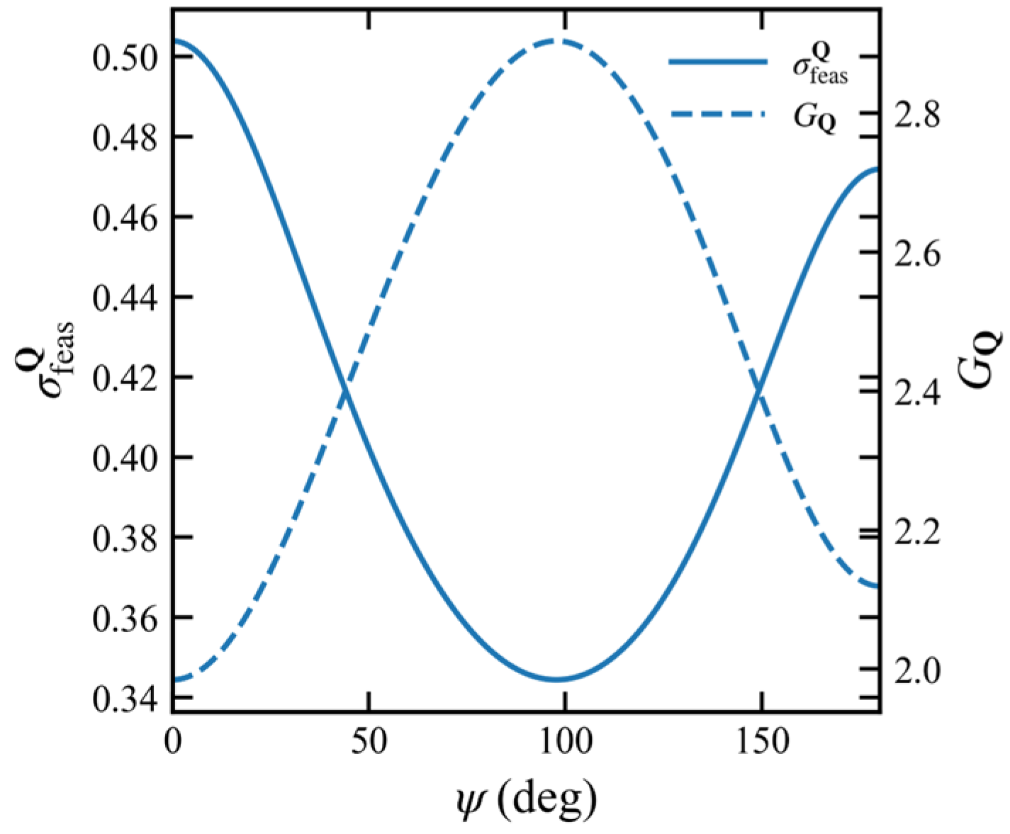
Equation (96) indicates that the weighted worst-case gain is the reciprocal of the weighted feasible sensitivity. Therefore, the fundamental cause of pronounced velocity amplification in the inverse mapping is not that the mechanism is literally “stuck” at that configuration, but rather that the feature-response intensity along the unique feasible direction becomes significantly weakened, i.e., ${\sigma }_{\mathrm{feas}}^Q(q)$ decreases, so that a larger generalized-velocity amplitude is required as compensation.

This observation also clarifies the interpretation of singularity in the present problem. Here, singular behavior is more appropriately understood as a degeneration of the weighted local feature mapping, rather than simply as a geometric dead point or a sudden disappearance of mobility. Consequently, the configuration at which inversion becomes most difficult does not necessarily coincide with the dead-point configuration. What truly governs the inversion difficulty is the local weighted amplification relation characterized by Equation (96).

It should further be emphasized that the weighted worst-case gain G_Q(q), as defined in Equations (93)–(96), is not intended to represent a universal, parameterization-independent geometric distance from the current configuration to the singular set. Rather, it is a local weighted amplification measure defined under the selected feature-space metric Q and generalized-velocity metric R_q. Specifically, it characterizes the maximum generalized-velocity magnitude required to realize a unit feature variation within the present metric-consistent formulation. Therefore, in the framework adopted here, singularity is more accurately reflected by the degeneration of the weighted local inverse mapping, namely, a vanishing feasible sensitivity together with an increasing worst-case gain. Once the metric is fixed, G_Q(q) can be used as an absolute amplification index for comparing different configurations of the same mechanism within the same modeling and weighting framework.

2.4.6. Damped Regularization and Homogeneous KKT Inverse Solution

Although Equation (91) provides a closed-form one-dimensional feasible inverse solution, Equation (96) shows that when ${\sigma }_{\mathrm{feas}}^Q(q)$ is small, the worst-case gain increases markedly, which may lead to excessive peaks in the generalized velocity and heightened sensitivity to numerical errors and modeling perturbations. To suppress this amplification effect while strictly satisfying the mechanism constraint, we further formulate the following weighted damped least-squares problem:

$$\underset{\dot{q}}{\min }\Vert J_f(q)\dot{q}-d_f{\Vert }_Q^2+\lambda (q){\dot{q}}^{⊺}{R}_q\dot{q}\hspace{0.33em}\hspace{0.33em}\hspace{0.33em}\mathrm{s}.\mathrm{t}.\hspace{0.33em}\hspace{0.33em}\hspace{0.33em}a{(q)}^{⊺}\dot{q}=0,$$

(97)

where λ(q) ≥ 0 is a configuration-dependent damping coefficient. The first term in Equation (97) is the weighted feature-velocity residual, which measures the mismatch between the target feature velocity d_f and the realizable feature velocity $J_f(q)\dot{q}$. The second term is a weighted generalized-velocity penalty used to suppress excessively large axial–twisting combined velocity amplitudes. Accordingly, Equation (97) establishes an explicit trade-off between tracking accuracy and bounded velocity magnitude.

Introducing the Lagrange multiplier μ, the corresponding Lagrangian is constructed as

$$\mathcal{L}(\dot{q},\mu )=\Vert J_f(q)\dot{q}-d_f{\Vert }_Q^2+\lambda (q){\dot{q}}^{⊺}{R}_q\dot{q}+2\mu a{(q)}^{⊺}\dot{q}.$$

(98)

Setting the partial derivatives of $\mathcal{L}$ with respect to $\dot{q}$ and μ to zero yields the fixed-dimension KKT linear system

$$\left[\begin{array}{cc}{J}_f{(q)}^{⊺}Q{J}_f(q)+\lambda (q)R_q& a(q)\\ a{(q)}^{⊺}& 0\end{array}\right]\left[\begin{array}{c}\dot{q}\\ \mu \end{array}\right]=\left[\begin{array}{c}{J}_f{(q)}^{⊺}Q{d}_f\\ 0\end{array}\right].$$

(99)

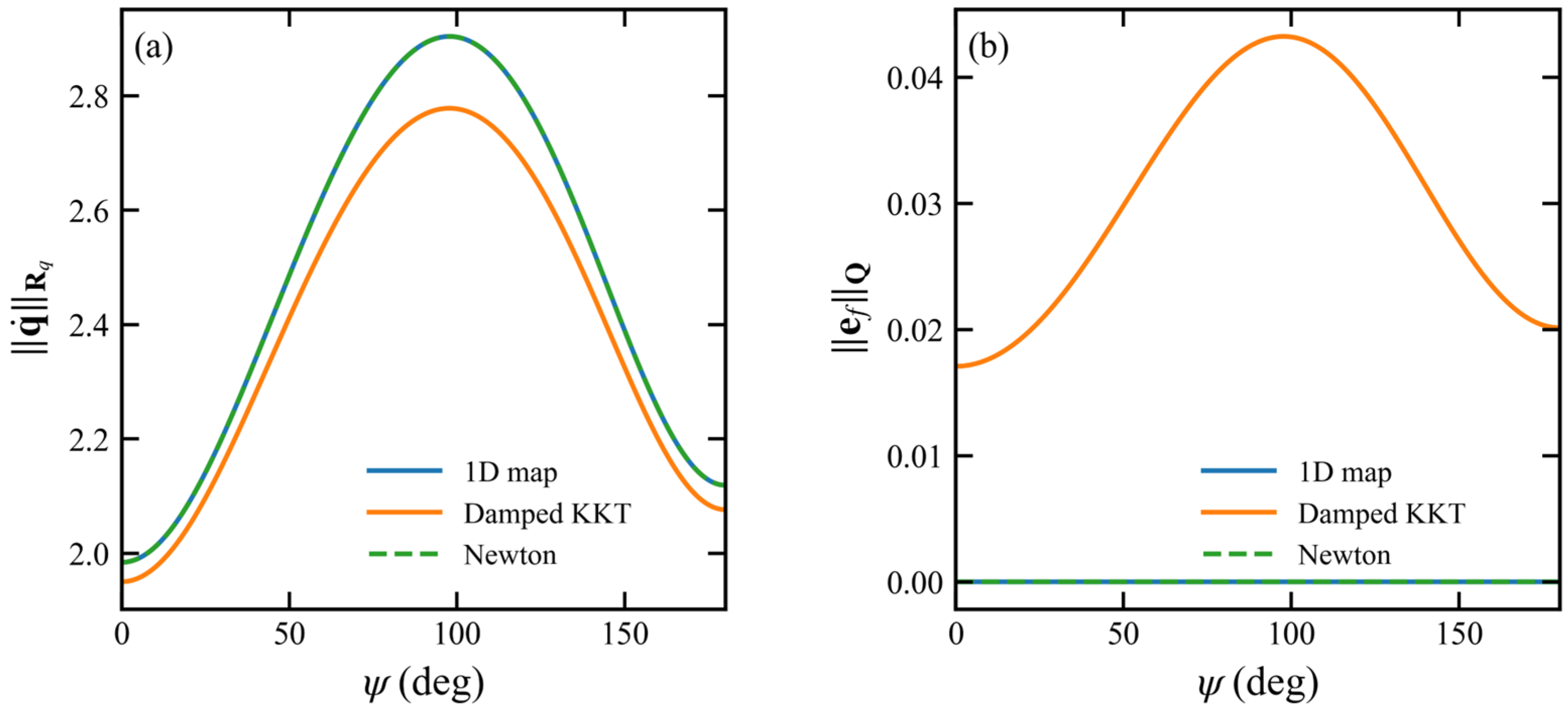
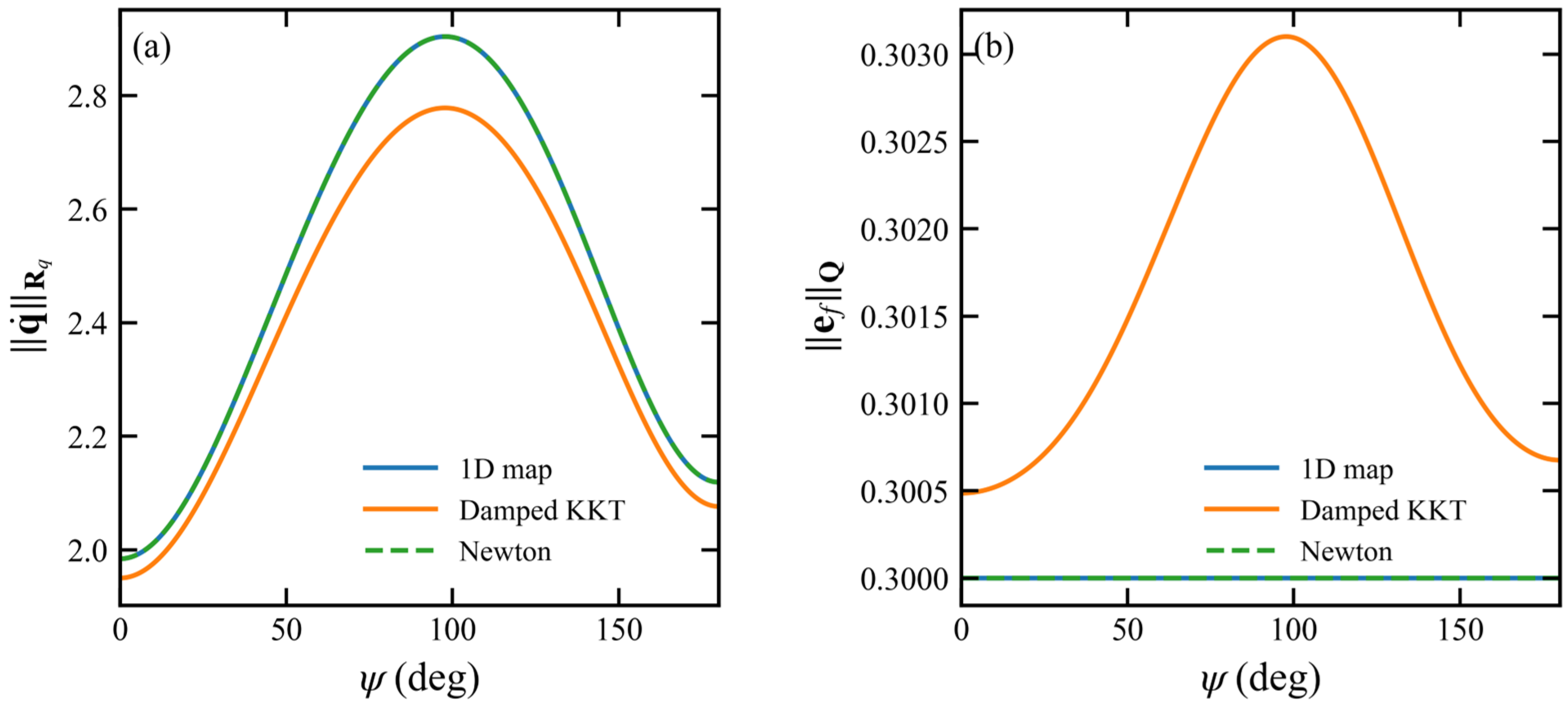
The unknowns in Equation (99) are only $\dot{q}\in {ℝ}^2$ and $\mu \in ℝ$. Thus, at each configuration, only one fixed-size 3 × 3 linear system needs to be solved. A key advantage of this formulation is that it does not require the explicit construction of a local pseudoinverse that may diverge in ill-conditioned regions; instead, it directly yields a damped bounded solution in the original pose variables under the explicit constraint.

Because the purpose of damping is to suppress velocity amplification in low-sensitivity regions, the damping coefficient is designed to depend on the weighted feasible sensitivity introduced above. Specifically, the following continuous scheduling law is adopted:

$$\lambda (q)={\lambda }_{\max }{\displaystyle \frac{{\sigma }_0}{{\sigma }_0+{\sigma }_{\mathrm{feas}}^Q(q)}},\hspace{0.33em}\hspace{0.33em}\hspace{0.33em}{\lambda }_{\max }>0,{\sigma }_0>0.$$

(100)

Equation (100) shows that when ${\sigma }_{\mathrm{feas}}^Q(q)$ is relatively large, λ(q) becomes small, so that the system approaches the unbiased weighted least-squares solution and preserves feature-velocity tracking accuracy. By contrast, when ${\sigma }_{\mathrm{feas}}^Q(q)$ is small, λ(q) increases, thereby strengthening the penalty on ${\dot{q}}^{⊺}{R}_q\dot{q}$, actively compressing the generalized-velocity amplitude and weakening the amplification effect.

Let the solution of Equation (99) be denoted by ${\dot{q}}_{\mathrm{KKT}}(q,d_f)$, and define the corresponding feature residual as

$$e_f=d_f-J_f(q){\dot{q}}_{\mathrm{KKT}}.$$

(101)

Therefore, the damped KKT inverse solution does not pursue an absolutely exact inverse mapping in the zero-residual sense. Instead, it accepts a small and controllable weighted feature residual in exchange for bounded generalized velocity, stability in the vicinity of dead points, and global numerical tractability. The emphasis of the present method is not on minimizing the residual at a single configuration, but on maintaining, throughout the entire workspace, an inverse-mapping framework that is interpretable, tunable, and bounded in the weighted sense.

3. Numerical Experiments and Results Analysis

3.1. Experimental Objectives and Validation Items

To validate the “line-field continuation–featurization–stable inverse solving” framework proposed in Section 2, this chapter conducts numerical experiments with emphasis on the following four aspects:

Consistency of constraint geometry: verify the analytical properties of the height function h(ψ) under the constant-length constraint and the corresponding equivalent pitch

$$p(\psi )\triangleq {\displaystyle \frac{\mathrm{d}h}{\mathrm{d}\psi }}.$$

(102)

Accuracy of line-field coefficient recovery: verify that the first-order truncated coefficients recovered from discrete rod-axis line-field samples via least squares agree with the analytically derived continuous coefficient curves over the entire pose interval.

Rationality of harmonic truncation: quantify the decay of harmonic energy with respect to order and confirm that higher-order harmonics lie at the level of machine precision, thereby supporting the effectiveness of first-order truncation.

Inverse-solution stability in near-ill-conditioned regions: in a full-domain sweep including dead points, compare the one-dimensional mapping closed-form inverse, the damped KKT inverse, and the conventional Newton method in terms of velocity magnitude and residual, and explain the origin of amplification and stability.

3.2. Experimental Setup and Parameter Configuration

All experiments in this chapter use the same mechanism parameters and weighting set tings to ensure consistent evaluation scales and comparability across tests. The pose variables are defined as $q={[h,\psi ]}^{⊺}$,where h is the platform height and ψ is the rotation angle about the z-axis. The tested mechanism is a six-limb axisymmetric parallel mechanism with n = 6 identical S–rod–S limbs and uniformly distributed anchors on both platforms. The parameter values are:

Upper/lower platform anchor radii: R_t = R_b = 35 mm;

Limb length: L = 140 mm.

To unify the relative magnitudes of the direction-type and moment-type feature components under the weighted norm, the normalization scale for moment-type entries in the feature weight matrix is chosen as L₀ = 140 mm.

The generalized-velocity metric is taken as

$$R_q\triangleq \mathrm{diag}\left({\displaystyle \frac{1}{{\dot{h}}_{\max }^2}},{\displaystyle \frac{1}{{\dot{\psi }}_{\max }^2}}\right),$$

(103)

Here ${\dot{\psi }}_{\max }=1\mathrm{rad}/\mathrm{s}$. From the constrained kinematics $\dot{h}=p(\psi )\dot{\psi }$, $\dot{h}$ attains its magnitude peak near ψ = 90°; therefore, this chapter sets ${\dot{h}}_{\max }=-9.3541\mathrm{mm}/\mathrm{s}$ to determine ρ_h.

3.3. Height–Rotation and Pitch–Rotation Relationships

Figure 5 shows the relationships between the height h(ψ) and the equivalent pitch p(ψ) as functions of the rotation angle ψ. The explicit relation h(ψ) follows directly from the constant-length constraint. Under the parameters used in this chapter, the curve reaches its maximum at ψ = 0°, h(0) = L = 140 mm, and its minimum at ψ = 180°,

$$h({180}^{°})=\sqrt{L^2-4R_t{R}_b}\approx 121.24\mathrm{mm}.$$

(104)

To characterize the instantaneous first-order response of height with respect to rotation under constrained motion, we define the equivalent pitch as p(ψ). From the velocity-level constraint, an analytical expression for p(ψ) can be obtained; its key feature is proportionality to $\sin \psi$. Consequently, at the dead points, p(0°) = p(180°) = 0.

As observed in Figure 5, the pitch is zero at both dead points and reaches its magnitude peak near intermediate poses. Moreover, p(ψ) exhibits an odd-symmetry structure, consistent with the first-order nature of the constrained motion.

3.4. Discrete Verification of Continuous Line-Field Coefficients

This section verifies the consistency between the line-field coefficients recovered from discrete rod-axis samples and the analytically derived continuous coefficient curves. Under first-order truncation, the line-field coefficient representation at each pose ψ ∈ [0°,180°] can be written as three groups, each being a 6D vector:

$$C(\psi )\leftrightarrow \{c_0(\psi ),c_1^c(\psi ),c_1^s(\psi )\},\hspace{0.33em}\hspace{0.33em}\hspace{0.33em}{c}_0,c_1^c,c_1^s\in {ℝ}^6,$$

(105)

where c₀ is the constant term, and $c_1^c$ and $c_1^s$ are the first-order cosine and sine terms, respectively.

For discrete verification, 22 pose samples are uniformly selected over the interval, including the two dead-point configurations at ψ = 0° and ψ = 180°. At each sampled pose, the discrete rod-axis line-field samples are used to recover c₀, $c_1^c$, and $c_1^s$ via least squares; in parallel, the analytical expressions are evaluated to obtain the corresponding continuous curves. In Figure 6a–d, solid lines represent the analytical continuous results, and circular markers denote the recovered values at the 22 sampled poses. The recovered discrete coefficients and the analytically derived continuous curves match closely across the full interval.

Figure 6a plots the weighted norms of the three coefficient groups versus ψ. The following observations can be made:

• $\Vert c_0(\psi ){\Vert }_Q$ remains dominant and decreases slowly with increasing ψ. This trend is consistent with the reduction in the axial direction component d_z in the constant term: in Figure 6b, d_z decreases from near 1 to approximately 0.86, leading to the corresponding decrease in $\Vert c_0{\Vert }_Q$.
• $\Vert c_1^c(\psi ){\Vert }_Q$ and $c_1^s(\psi ){\Vert }_Q$ are nearly identical over the entire interval, and both increase monotonically with ψ. This “equal-magnitude, orthogonal-phase” behavior indicates that when the circumferential first-order content is expanded on the orthogonal basis $\{\cos \theta ,\sin \theta \}$, the energy is distributed approximately evenly across the two orthogonal directions. Meanwhile, the increasing pose angle strengthens the first-order circumferential component while preserving a regular orthogonal structure.

Figure 6b–d show the variations of c₀(ψ), $c_1^c(\psi )$, and $c_1^s(\psi )$ across the six Plücker components. For the ideal axisymmetric model, some components are analytically zero. In the corresponding subplots, the vertical-axis level is around 10⁻¹⁷ to 10⁻¹⁵; the small random fluctuations of discrete markers at these levels are attributable to floating-point residuals rather than modeling errors. For the structural components that are analytically nonzero, the discrete markers align with the analytical curves and exhibit clear pose-dependent trends. Specifically:

• c₀(ψ) (Figure 6b): d_z decreases monotonically with ψ; m_z approaches 0 near the endpoints and reaches a negative peak at intermediate poses, forming a characteristic concave-down single-peak trend (dominated by $\sin \psi$).
• $c_1^c(\psi )$ (Figure 6c): for the first-order cosine term, d_x and d_y vary smoothly (monotone/convex); m_x and m_y serve as primary contributors and exhibit pronounced trends such as “increase then decrease” or monotone variation, reflecting strengthening and redistribution of the first-order circumferential component in moment-type entries. The recovered discrete points match the analytical curves.
• $c_1^s(\psi )$ (Figure 6d): for the first-order sine term, d_x, d_y, m_x, and m_y also show smooth and continuous pose trends. Compared with $c_1^c$, the component allocation differs due to phase orthogonality. Together with the near-overlap of the norms in Figure 6a, these results indicate that the first-order energy increases with pose angle, while the energy carried by the $\cos \theta$ and $\sin \theta$ bases remains nearly balanced.

In summary, Figure 6a–d demonstrate, at both the norm level and the component level, that over the full interval [0°,180°] the recovered $c_0$, $c_1^c$, and $c_1^s$ agree closely with the analytical continuous coefficients, and follow stable, interpretable pose-dependent patterns.

3.5. Decay of the Feature Energy Spectrum

To assess the rationale of first-order harmonic truncation and the pose-dependent allocation of spectral energy, this section examines five representative poses:

$$\psi \in \{0^{\circ },{45}^{\circ },{90}^{\circ },{135}^{\circ },{180}^{\circ }\},$$

(106)

and computes the distribution of harmonic-coefficient energy as a function of harmonic order k.

$$E_k(\psi )\triangleq {‖c_k(\psi )‖}_Q^2,$$

(107)

Figure 7 shows the decay curve of the weighted energy E_k with respect to k, with a vertical dashed line indicating the boundary between k = 1 and higher-order components. The results indicate that energy is concentrated in low-order terms. When k ≥ 2, the energy rapidly drops to numerical residual levels, implying that for the ideal axisymmetric model the higher-order harmonics contribute negligibly to the line-field representation, consistent with the modeling assumption of first-order truncation.

Meanwhile, the five curves in Figure 7 exhibit a clear increasing trend at k = 1 as the pose angle increases: from ψ = 0° to ψ = 180°, the first-order energy becomes progressively larger. This suggests that as the pose departs further from the aligned configuration, the circumferential variation in the line field becomes stronger, and a larger first-order harmonic is required to capture this circumferential change. This observation corroborates the monotonic increase of $\Vert c_1^c(\psi ){\Vert }_Q$ and $\Vert c_1^s(\psi ){\Vert }_Q$ with ψ reported in Section 3.4: the growth of first-order spectral energy manifests, at the coefficient-norm level, as a synchronous increase in the magnitudes of the first-order coefficient blocks.

Therefore, Figure 7 not only validates the truncation rationale that higher-order harmonics can be neglected, but also reveals how pose variation affects the allocation of low-order energy: the constant term (k = 0) captures the dominant axial structure, the first-order term (k = 1) strengthens with increasing ψ and carries more circumferential variation, whereas energy at k ≥ 2 remains at numerical residual levels.

3.6. Velocity-Inversion Simulation Analysis

3.6.1. Test Cases and Inverse-Solver Settings

For the inverse problem of feature velocity in the line-field feature space, two test cases are constructed and the numerical stability of the inverse solutions is compared against the conventional Newton iteration. To obtain smooth full-domain curves and to facilitate the computation of pose-wise statistics (e.g., the median over the pose set), the pose angle is swept over ψ ∈ [0°,180°] with a step size of 0.1°.

Case 1: Fully reachable target feature velocity.

To ensure reachability at all poses, the target feature velocity is chosen as the Q-normalized form of the admissible image direction:

$${\dot{f}}_d(q)=F_0{\displaystyle \frac{v(q)}{{‖v(q)‖}_0}},$$

(108)

where F₀ is the amplitude. In this experiment, F₀ = 1. This construction guarantees ${\dot{f}}_d(q)\in \mathrm{span}\{v(q)\}$, and the residual can theoretically be driven to zero.

Case 2: Target feature velocity with an unreachable component.

On top of Case 1, an additional component that is Q-orthogonal to v is superimposed. We take the candidate direction

$$j_h\triangleq \mathrm{vec}(C_h),$$

(109)

and perform Q-orthogonalization:

$$e_{\perp }=j_h-v{\displaystyle \frac{v^{\top }Q{j}_h}{v^{\top }Qv}},\hspace{0.33em}\hspace{0.33em}\hspace{0.33em}{\widehat{e}}_Q={\displaystyle \frac{e_{\perp }}{\parallel e_{\perp }{\parallel }_Q}}.$$

(110)

The Case-2 target is then defined as

$${\dot{f}}_d(q)=F_0{\displaystyle \frac{v(q)}{{‖v(q)‖}_Q}}+\beta {\widehat{e}}_Q(q),$$

(111)

where β is the amplitude of the unreachable component. In this experiment β = 0.3. Since ${\widehat{e}}_Q{\perp }_{Q}v$, any one-dimensional least-squares solution restricted to the admissible direction cannot cancel this component; therefore, the theoretical lower bound of the minimum residual is β.

Both cases are evaluated using three inverse schemes: the one-dimensional mapping method (Equations (90) and (91)), the damped KKT inverse (Equations (97)–(101)), and the conventional Newton iteration. For the damping schedule in Equation (100), we set λ_max = 10⁻² and choose σ₀ as the median over the full pose set. From Figure 8, σ₀ = 0.398. The global minimum feasible sensitivity occurs at ψ ≈ 97.7°, yielding the peak worst-case gain $G_{\max }^Q=2.904$. Near the endpoint dead points, ${\sigma }_{\mathrm{feas}}^Q$ is not minimal; for example, at ψ = 0°, ${\sigma }_{\mathrm{feas}}^Q=0.504$ and the corresponding gain is 1.985, which is clearly lower than the peak. This indicates that, under the “feature velocity–admissible velocity” mapping, inverse difficulty is governed primarily by ${\sigma }_{\mathrm{feas}}^Q$, rather than being determined directly by the geometric dead points in the traditional sense.

3.6.2. Results and Discussion for Case 1

From the analytical solution of the one-dimensional admissible mapping (Equation (90)), the generalized-velocity magnitude under the R_q-metric is

$${‖\dot{q}‖}_{R_q}=\mid z^{*}\mid ={\displaystyle \frac{F_0}{{\sigma }_{\mathrm{feas}}^Q(\psi )}},\hspace{0.33em}\hspace{0.33em}\hspace{0.33em}(F_0=1).$$

(112)

Therefore, the $\Vert \dot{q}{\Vert }_{R_q}$ curve obtained by the one-dimensional method has the same trend as the worst-case gain curve in Figure 8: the smaller the feasible sensitivity, the weaker the mapping, and the larger the generalized-velocity magnitude required to produce a unit feature velocity.

We further compare the three inverse solvers (Figure 9):

• One-dimensional mapping method: $\Vert \dot{q}{\Vert }_{R_q}$ reaches its maximum value 2.904 at ψ ≈ 97.7°, while it is 1.985 near ψ = 0°. This shows that, in Case 1, the worst pose is associated with the sensitivity trough rather than the geometric dead points.
• Damped KKT: the curve lies below that of the one-dimensional method overall, and its peak reduction occurs at the same location as the sensitivity trough. The peak value is reduced to 2.778, corresponding to a peak-shaving ratio of approximately 4.32%. A further comparison of the full-pose mean values shows that the one-dimensional method yields an average $\Vert \dot{q}{\Vert }_{R_q}=2.492$, whereas the damped KKT yields 2.413, i.e., an average reduction of approximately 3.18%.
• Conventional Newton iteration: apart from producing NaNs at the dead points, its curve is essentially identical to that of the one-dimensional method.

In terms of residuals, Figure 9 shows that the one-dimensional method and the Newton method (excluding the dead points) achieve zero residual, while the damped KKT introduces a nonzero residual and attains its maximum at ψ ≈ 97.7°:

$$\Vert e_f{\Vert }_{Q,\max }^{\mathrm{KKT}}=0.043244.$$

(113)

The coincidence of the residual peak and the velocity peak-shaving location reflects the fundamental role of damping regularization: allowing a controlled tracking error in exchange for bounded velocities and peak suppression.

Because the Case-1 target direction is strictly aligned with v(q), the admissible image space is one-dimensional and the damped KKT effectively performs amplitude compression along the same direction. Defining

$$\alpha (q)\triangleq {\displaystyle \frac{z^{ \mathrm{KKT}}(q)}{z^{*}(q)}}\in (0,1],\hspace{0.33em}\hspace{0.33em}\hspace{0.33em}{z}^{*}={\displaystyle \frac{1}{{\sigma }_{\mathrm{feas}}^{\mathrm{Q}}(\psi )}}\left(F_0=1\right).$$

(114)

the residual satisfies the exact relation

$$\Vert e_f{\Vert }_Q=\left|\begin{array}{c}1-\alpha (q)\end{array}\right|.$$

(115)

Hence, at ψ ≈ 97.7°, a peak-shaving ratio of 4.32% corresponds to a residual peak of approximately 0.0432, consistent with the simulation.

Quantitative comparisons for representative poses (including the dead points ψ = 0° and 180°) are summarized in

Table 1. Quantitative comparison of inverse solvers for Case 1.

ψ (deg)	$\Vert \dot{\mathbf{q}}{\Vert }_{{\mathbf{R}}_{\mathit{q}}}$ (Newt)	$\Vert {\mathbf{e}}_{\mathit{f}}{\Vert }_{\mathbf{Q}}$ (Newt)	$\Vert \dot{\mathbf{q}}{\Vert }_{{\mathbf{R}}_{\mathit{q}}}$ (1D)	$\Vert {\mathbf{e}}_{\mathit{f}}{\Vert }_{\mathbf{Q}}$ (1D)	$\Vert \dot{\mathbf{q}}{\Vert }_{{\mathbf{R}}_{\mathit{q}}}$ (KKT)	$\Vert {\mathbf{e}}_{\mathit{f}}{\Vert }_{\mathbf{Q}}$ (KKT)
0	NaN	NaN	1.984556	0	1.950649	0.017085
0.1	1.984558	0	1.984558	0	1.950652	0.017085
0.5	1.984624	0	1.984624	0	1.950714	0.017087
179.5	2.119342	0	2.119342	0	2.076660	0.020140
179.9	2.119255	0	2.119255	0	2.076579	0.020138
180	NaN	NaN	2.119252	0	2.076575	0.020137

. The tabulated results further indicate that the Newton method fails (NaNs) at dead points, whereas both the one-dimensional mapping method and the damped KKT formulation remain computable and numerically stable there. Taken together, these results suggest that near dead points the amplification is not necessarily extreme (since ${\sigma }_{\mathrm{feas}}^Q(\psi )$ is not minimal there); rather, the primary risk stems from the numerical pathology of iterative schemes, not from an inherent “unsolvability” of the mapping.

3.6.3. Results and Discussion for Case 2

In Case 2, a Q-orthogonal unreachable component $\beta {\hat{\mathrm{e}}}_Q(\psi )$ is added to the reachable target of Case 1, with β = 0.3 and ${\widehat{e}}_Q{\perp }_{Q}v$. The least-squares scalar solution of the one-dimensional mapping method is

$$z^{\ast }={\displaystyle \frac{v^{⊺}Q{\dot{f}}_d}{v^{⊺}Qv}}={\displaystyle \frac{v^{⊺}Q\left(F_0\frac{v}{\Vert v{\Vert }_Q}+\beta {\widehat{e}}_Q\right)}{v^{⊺}Qv}}={\displaystyle \frac{F_0}{\Vert v{\Vert }_Q}}={\displaystyle \frac{F_0}{{\sigma }_{\mathrm{feas}}^Q(\psi )}}.$$

(116)

Thus, the unreachable component does not change the optimal admissible velocity magnitude; it only appears in the final residual. From a velocity-control viewpoint, this implies that when the unreachable component is strictly Q-orthogonal to v, the optimal admissible motion under least squares is still fully determined by ${\sigma }_{\mathrm{feas}}^Q(\psi )$. Accordingly, the generalized-velocity curve in Figure 10a coincides with that of Case 1 (Figure 9a).

For residuals, the Case-2 construction ensures that the unreachable component is strictly Q-orthogonal to the admissible image v. Therefore:

• One-dimensional mapping: the reachable component can be matched exactly, but the unreachable component cannot be generated by any admissible velocity. Hence, the theoretical lower bound of the minimum residual is β, which appears as the horizontal line at 0.3 in Figure 10b.
• Damped KKT: amplitude compression α(ψ) introduces an additional error 1 − α(ψ) on the reachable direction. Since the unreachable error β and the reachable-direction error are Q-orthogonal, the total residual satisfies

  $$\Vert e_f{\Vert }_Q=\sqrt{{\beta }^2+{\left(1-\alpha (\psi )\right)}^2}.$$

  (117)

Consequently, the curve exhibits only a mild elevation above β, reaching its maximum at ψ ≈ 97.7° (where σ is minimal and damping is strongest):

$$\Vert e_f{\Vert }_{Q,\max }^{\mathrm{KKT}}=0.303101.$$

The increase relative to β is only 0.003101 (about 1.03%), indicating that under the current damping setting, the damped KKT achieves peak shaving and dead-point stability at a very small additional tracking cost.

• Conventional Newton iteration: it fails at ψ = 0° and 180°, indicating that the failure is unrelated to reachability of the target and is instead closely tied to numerical ill-conditioning at dead points.

Quantitative comparisons for representative poses are summarized in

Table 2. Quantitative comparison of inverse solvers for Case 2.

ψ (deg)	$\Vert \dot{\mathbf{q}}{\Vert }_{{\mathbf{R}}_{\mathit{q}}}$ (Newt)	$\Vert {\mathbf{e}}_{\mathit{f}}{\Vert }_{\mathbf{Q}}$ (Newt)	$\Vert \dot{\mathbf{q}}{\Vert }_{{\mathbf{R}}_{\mathit{q}}}$ (1D)	$\Vert {\mathbf{e}}_{\mathit{f}}{\Vert }_{\mathbf{Q}}$ (1D)	$\Vert \dot{\mathbf{q}}{\Vert }_{{\mathbf{R}}_{\mathit{q}}}$ (KKT)	$\Vert {\mathbf{e}}_{\mathit{f}}{\Vert }_{\mathbf{Q}}$ (KKT)
0	NaN	NaN	1.984556	0.300000	1.950649	0.300486
0.1	1.984558	0.300000	1.984558	0.300000	1.950652	0.300486
0.5	1.984624	0.300000	1.984624	0.300000	1.950714	0.300486
179.5	2.119342	0.300000	2.119342	0.300000	2.076660	0.300675
179.9	2.119255	0.300000	2.119255	0.300000	2.076579	0.300675
180	NaN	NaN	2.119252	0.300000	2.076576	0.300675

. The tabulated results further confirm that even when the target contains unreachable components, the one-dimensional mapping method stably outputs the optimal reachable-part velocity magnitude, with residual strictly remaining at β. The damped KKT remains computable at dead points and slightly increases residual near the sensitivity trough (from 0.300000 to 0.303101), exhibiting a clear regularization trade-off.

3.7. Robustness Under Mild Geometric Perturbations

To further examine the robustness of the proposed line-field featurization and stable inverse-solving framework under mild geometric imperfections, this section analyzes the statistical results of platform-radius perturbations, rod-length perturbations, and anchor-offset perturbations at three perturbation levels, namely 1%, 2%, and 5%. For each perturbation type and level, 200 Monte Carlo trials are conducted. The analysis focuses on five quantities: the maximum first-order fitting error, the mean second-order leakage, the peak worst-case gain, the peak-shaving ratio, and the high-order harmonic ratio.

Let $f^{(s)}(\psi )$ denote the true line-field feature in the s-th trial, and let ${\widehat{f}}_{N_h=1}^{(s)}(\psi )$ denote its first-order truncated reconstruction. The statistical quantities used in this section are defined as follows:

$${\epsilon }_{\mathrm{fit},\max }^{(s)}=\underset{\psi \in [0^{\circ },{180}^{\circ }]}{\max }{\displaystyle \frac{{‖f^{(s)}(\psi )-{\widehat{f}}_{N_h=1}^{(s)}(\psi )‖}_Q}{{‖f^{(s)}(\psi )‖}_Q}}\times 100\%,$$

(118)

$${\overline{\eta }}_2^{(s)}={\displaystyle \frac{1}{N_{\psi }}}{\displaystyle \sum _{\psi }\frac{E_2^{(s)}(\psi )}{{\displaystyle \sum _{k=0}^2{E}_k^{(s)}}(\psi )}}\times 100\%,$$

(119)

$$G_{Q,\max }^{(s)}=\underset{\psi \in [0^{°},{180}^{°}]}{\max }{G}_Q^{(s)}(\psi ),$$

(120)

$${\Gamma }_{\mathrm{shave}}^{(s)}=\left(1-{\displaystyle \frac{{\max }_{\psi }{‖{\dot{q}}_{\mathrm{KKT}}^{(s)}(\psi )‖}_{R_q}}{{\max }_{\psi }{‖{\dot{q}}_{\mathrm{lD}}^{(s)}(\psi )‖}_{R_q}}}\right)\times 100\%,$$

(121)

$${\overline{\eta }}_{\ge 2}^{(s)}={\displaystyle \frac{1}{N_{\psi }}}{\displaystyle \sum _{\psi }\frac{{\displaystyle \sum _{k=2}^K{E}_k^{(s)}}(\psi )}{{\displaystyle \sum _{k=0}^K{E}_k^{(s)}}(\psi )}}\times 100\%,\hspace{0.33em}\hspace{0.33em}\hspace{0.33em}K=10.$$

(122)

Here, ${\epsilon }_{\mathrm{fit},\max }$ measures the maximum relative fitting error of the first-order truncation over the full pose interval, ${\overline{\eta }}_2$ quantifies the mean second-order harmonic leakage, $G_{Q,\max }$ characterizes the worst local amplification level, ${\Gamma }_{\mathrm{shave}}$ evaluates the peak-suppression effect of the damped KKT inverse, and ${\overline{\eta }}_{\ge 2}$ describes the average contribution of higher-order harmonics.

Figure 11 shows the statistical distribution of the maximum first-order fitting error under the three perturbation families. It can be seen that both platform-radius perturbations and anchor-offset perturbations cause ${\epsilon }_{\mathrm{fit},\max }$ to increase monotonically with the perturbation level, whereas the error under rod-length perturbations remains at the numerical-residual level throughout. Specifically, for platform-radius perturbations, the mean value of ${\epsilon }_{\mathrm{fit},\max }$ increases from 0.3918% ± 0.1036% at 1% to 0.7800% ± 0.1981% at 2%, and further to 1.9964% ± 0.5092% at 5%. For anchor-offset perturbations, the corresponding values rise from 0.5994% ± 0.1839% to 1.2471% ± 0.3538% and 2.9511% ± 0.8836%. In contrast, the error under rod-length perturbations stays at approximately 5.0 × 10⁻¹⁴%, which can be regarded as numerical noise. This indicates that, within the present featurization framework, the dominant source of first-order degradation is not a mere change in scale, but rather a loss of circumferential symmetry, with anchor-offset perturbations being the most sensitive.

Figure 12 presents the mean second-order leakage ${\overline{\eta }}_2$, whose trend is largely consistent with that of Figure 11. For platform-radius perturbations, ${\overline{\eta }}_2$ increases from 0.000283% ± 0.000159% to 0.001155% ± 0.000641% and 0.007275% ± 0.003708%. For anchor-offset perturbations, it increases from 0.000457% ± 0.000344% to 0.002066% ± 0.001512% and 0.010817% ± 0.008647%. These results show that mild geometric perturbations do activate higher-order harmonics that are at residual levels in the ideal axisymmetric model. Nevertheless, for perturbation levels of 1–2%, the leakage remains relatively small and does not overturn the dominance of the low-order structure. Again, rod-length perturbations keep ${\overline{\eta }}_2$ at the 10⁻³⁰% level, indicating that their effect on the circumferential spectrum is negligible under the present setting.

Figure 13 shows the statistics of the peak worst-case gain G_Q,max. In the nominal model, the peak value is 2.9035. Under platform-radius perturbations, the corresponding values are 2.9043 ± 0.0051, 2.9023 ± 0.0095, and 2.9063 ± 0.0237 for 1%, 2%, and 5%, respectively. Under anchor-offset perturbations, they are 2.90349 ± 0.00004, 2.90339 ± 0.00018, and 2.90258 ± 0.00113. Under rod-length perturbations, the values remain at 2.9035 to four significant digits. Therefore, although geometric perturbations clearly affect the accuracy of the low-order feature representation, they do not cause a substantial drift in the peak worst-case gain. In other words, the overall amplification level at the most unfavorable pose remains nearly unchanged under mild perturbations.

Figure 14 reports the peak-shaving ratio Γ_shave of the damped KKT inverse. In the nominal case, the peak-shaving ratio is 4.3244%. For platform-radius perturbations, the corresponding values are 4.3266% ± 0.0147%, 4.3213% ± 0.0275%, and 4.3331% ± 0.0691%. For anchor-offset perturbations, they are 4.3245% ± 0.0002%, 4.3242% ± 0.0005%, and 4.3216% ± 0.0033%. For rod-length perturbations, they are 4.3245% ± 0.0026%, 4.3242% ± 0.0049%, and 4.3251% ± 0.0124%. These results indicate that, across all perturbation types and levels considered here, the peak-suppression capability of the damped KKT inverse remains highly stable. Thus, while mild geometric perturbations may alter the accuracy of the feature representation, the regularization mechanism for suppressing velocity peaks remains effective.

Figure 15 shows the average high-order harmonic ratio ${\overline{\eta }}_{\ge 2}$. Under the current statistical definition, the baseline value in the nominal model is approximately 53.545%. For platform-radius perturbations, the corresponding values are 53.5453% ± 0.0114%, 53.5488% ± 0.0220%, and 53.5501% ± 0.0546%. For rod-length perturbations, they are 53.5452% ± 0.0105%, 53.5436% ± 0.0196%, and 53.5467% ± 0.0507%. By contrast, anchor-offset perturbations exhibit a clearer increasing trend, from 53.5693% ± 0.0162% to 53.6376% ± 0.0658%, and further to 54.0978% ± 0.3716% at the 5% level. This suggests that, under the present statistical measure, the most pronounced redistribution of high-order spectral energy is induced by phase-type circumferential perturbations, whereas platform-radius and rod-length perturbations exert much weaker influence on the higher-order spectrum.

Taken together, Figure 11, Figure 12, Figure 13, Figure 14 and Figure 15 reveal a clear hierarchy in the influence of mild geometric perturbations. Platform-radius perturbations and anchor-offset perturbations primarily degrade the low-order accuracy of the line-field representation and activate higher-order harmonics, with anchor-offset perturbations being the most influential because they directly destroy circumferential phase uniformity. Rod-length perturbations, in contrast, remain weak in the present setting and scarcely affect the dominant spectral structure. At the same time, both the peak worst-case gain and the peak-shaving ratio remain remarkably stable under all perturbation types, indicating that the proposed stable inverse-solving framework is robust to mild geometric imperfections.

Table 3. Statistical summary of robustness metrics under mild geometric perturbations.

Perturbation Type	Level	Max First-Order Fit Error/%	Mean Second-Order Leakage/%	Peak GQ	Peak-Shaving Ratio/%	High-Order Harmonic Ratio/%
Platform radius	1%	0.3918 ± 0.1036	0.000283 ± 0.000159	2.9043 ± 0.0051	4.3266 ± 0.0147	53.5453 ± 0.0114
Platform radius	2%	0.7800 ± 0.1981	0.001155 ± 0.000641	2.9023 ± 0.0095	4.3213 ± 0.0275	53.5488 ± 0.0220
Platform radius	5%	1.9964 ± 0.5092	0.007275 ± 0.003708	2.9063 ± 0.0237	4.3331 ± 0.0691	53.5501 ± 0.0546
Rod length	1%	5.0472 × 10−14 ± 1.2822 × 10−15	3.2683 × 10−30 ± 2.0494 × 10−32	2.90354 ± 0.00060	4.3245 ± 0.0026	53.5452 ± 0.0105
Rod length	2%	5.0312 × 10−14 ± 1.2595 × 10−15	3.2675 × 10−30 ± 2.3042 × 10−32	2.90345 ± 0.00111	4.3242 ± 0.0049	53.5452 ± 0.0105
Rod length	5%	5.0505 × 10−14 ± 1.3186 × 10−15	3.2641 × 10−30 ± 2.4937 × 10−32	2.90365 ± 0.00288	4.3251 ± 0.0124	53.5467 ± 0.0507
Anchor offset	1%	0.5994 ± 0.1839	0.000457 ± 0.000344	2.90349 ± 0.00004	4.3245 ± 0.0002	53.5693 ± 0.0162
Anchor offset	2%	1.2471 ± 0.3538	0.002066 ± 0.001512	2.90339 ± 0.00018	4.3242 ± 0.0005	53.6376 ± 0.0658
Anchor offset	5%	2.9511 ± 0.8836	0.010817 ± 0.008647	2.90258 ± 0.00113	4.3216 ± 0.0033	54.0978 ± 0.3716

further clarifies that the representation-level deviations and the inverse-level stability metrics have different sensitivities. The former, including the maximum first-order fitting error, the mean second-order leakage, and the high-order harmonic ratio, are much more sensitive to the destruction of circumferential symmetry. The latter, namely the peak worst-case gain and the peak-shaving ratio, remain nearly invariant. This indicates that mild geometric perturbations first affect the strict low-order accuracy of the line-field representation, rather than immediately destroying the boundedness or regularization effect of the inverse solution.

Overall, within the 1–5% perturbation range considered here, platform-radius perturbations and anchor-offset perturbations gradually weaken the strict exactness of the low-order representation in the ideal axisymmetric model and introduce observable higher-order spectral leakage, with anchor-offset perturbations producing the strongest effect, platform-radius perturbations the second strongest, and rod-length perturbations the weakest. Nevertheless, even at the 5% perturbation level, both the peak worst-case gain and the peak-shaving ratio remain stable. Therefore, the proposed line-field featurization and stable inverse-solving framework is not only effective in the ideal axisymmetric model, but also robust under mild geometric imperfections.

4. Discussion

Instantaneous kinematic mapping in parallel mechanisms is most commonly analyzed through the Jacobian. Classical studies have shown that closed-chain architectures exhibit velocity amplification and degraded controllability in the neighborhood of singular configurations, and have established complementary interpretations from algebraic rank conditions and geometric line-system viewpoints [6,7,8]. In addition, studies on kinematically redundant planar parallel manipulators and singularity-free trajectory planning have shown that redundancy can be exploited to enlarge the usable workspace, avoid singular configurations, and improve actuation performance [28,29]. In the present work, we adopt a line-geometric and screw-theoretic formulation, treating the limb axes as the primary carriers of the mechanism’s geometric state and investigating the velocity mapping directly in a feature space. This viewpoint is consistent with the unifying description of motion and constraint afforded by screw theory [10,11,12,13], and it provides a natural geometric entry point for axisymmetric parallel mechanisms.

A central premise of the proposed framework is that axisymmetric, uniformly distributed anchor layouts impose strong structure on the circumferential line field. The analytical derivations show that each component of the normalized Plücker line field contains only a constant term and first-order harmonics. Consequently, first-order truncation introduces no truncation error in the ideal model. The numerical results in Section 3 further show that the coefficients recovered from discrete sampling agree closely with the analytical curves over the full pose interval, and that the spectral energy of higher-order harmonics decays to numerical residual levels. These results indicate that the line-field feature vector achieves effective dimensionality reduction while preserving geometric meaning, thereby enabling analytical differentiation and efficient inverse computation.

The same structure also helps clarify the physical meaning of dead points. In conventional discussions, dead points are often associated with non-traversable singular configurations. Under the constant-length constraint considered here, however, the velocity constraint restricts admissible generalized velocities to a one-dimensional subspace. At a dead point, the height-rate component becomes locked at the velocity level, while the admissible generalized-velocity subspace itself remains one-dimensional and the feature mapping still retains a first-order response to the rotation angle. This means that the dominant issue near dead points is expressed through inverse amplification caused by reduced effective sensitivity of the input–output mapping. From this perspective, the dead point and the most ill-conditioned pose need not coincide.

This distinction is important when comparing the present formulation with the redundancy-oriented literature. In works such as [28,29], singularity handling is primarily discussed at the mechanism or trajectory level, for example through workspace improvement, singularity-free path generation, or reduction in actuation effort. By contrast, the quantity G_Q introduced here is defined under fixed feature-space and generalized-velocity metrics, and it measures the local amplification required to realize a prescribed feature velocity at a given pose. Accordingly, G_Q should be interpreted as a metric-dependent local inverse-amplification index. It is well suited for comparing configurations within the same modeling and weighting framework, while workspace-based and trajectory-level redundancy strategies remain complementary tools for global task planning [28,29].

Exploiting the one-dimensional admissible-motion structure, we define the feasible sensitivity ${\sigma }_{\mathrm{feas}}^Q$ and derive its reciprocal relationship with the worst-case gain G_Q. The numerical results show that the minimum feasible sensitivity occurs at approximately 97.7°, where the worst-case gain also reaches its peak, whereas the sensitivities at the two dead-point endpoints are clearly higher. This demonstrates that inverse difficulty is governed by mapping strength rather than by the dead-point locations themselves. Because the feature vector contains both direction-type and moment-type components, a weighted metric is introduced to avoid implicit bias caused by dimensional inconsistency. This choice aligns with the motivation for dimensionally homogeneous Jacobians [21] and gives the sensitivity evaluation and damping schedule a more stable physical scale.

On the numerical side, the constrained damped least-squares problem is cast as a fixed-size KKT linear system, which avoids the divergence that iterative schemes may encounter in ill-conditioned regions. For reachable targets, the damped KKT solver trades a small residual for peak-velocity suppression, reducing the peak generalized-velocity norm by about 4.32% and the full-pose mean by about 3.18%. The reduction occurs at the same pose where the feasible sensitivity reaches its trough. For targets containing an unreachable component, the one-dimensional admissible inverse preserves the optimal reachable part exactly, and the residual remains at the theoretical lower bound β. The damped KKT inverse only introduces a slight additional increase in residual near the sensitivity trough, with the peak residual rising to 0.303101 when β = 0.3, corresponding to an increase of about 1.03%. These results show that the present formulation achieves a clear and controllable trade-off between amplification suppression and tracking accuracy.

Compared with singularity-robust inverse solutions based on damping and regularization [22], the present feasible-sensitivity formulation provides an interpretable basis for parameter scheduling. Compared with strategies that avoid ill-conditioned regions through reparameterization [23] or through redundancy-based trajectory planning [29], the present approach emphasizes obtaining bounded inverse responses directly under the original pose variables and constraints. This makes it suitable for integration with constraint-based control formulations and for local evaluation of inverse amplification risk.

The perturbation results in Section 3.7 further indicate that the proposed framework remains robust under mild geometric imperfections. Platform-radius perturbations and anchor-offset perturbations produce observable increases in first-order fitting error and second-order leakage, with anchor-offset perturbations exhibiting the strongest sensitivity because they directly disturb the circumferential phase structure. Rod-length perturbations remain weak in the present setting and have negligible influence on the dominant low-order spectrum. At the same time, the peak worst-case gain and the peak-shaving ratio remain nearly unchanged across all perturbation families and levels considered. These observations indicate that mild geometric imperfections primarily affect the strict low-order exactness of the feature representation, while the boundedness and regularization effect of the inverse solver remain stable.

Several limitations remain. The current derivations assume ideal axisymmetry and rigid-body behavior in the main model, and the feature weights and damping parameters are selected empirically rather than adaptively. The present numerical study validates coefficient recovery, spectral decay, inverse amplification, and robustness of feature-velocity inversion, whereas experimental verification on physical prototypes and extension to higher-order dynamic quantities remain to be established. Future work may incorporate higher-order harmonics as explicit descriptors of geometric imperfections, combine the proposed representation with parameter identification and calibration, and exploit the resulting sensitivity measures in risk-aware planning and gain design.

5. Conclusions

This paper proposed a line-field-based low-dimensional representation and stable inverse-solving framework for an axisymmetric parallel mechanism. By introducing a normalized Plücker line-field feature vector, the rod-axis assembly was transformed into an analytically tractable feature-space description, from which the continuous coefficient curves and the corresponding feature Jacobian were derived in closed form.

The results show that the inverse difficulty is governed primarily by the feasible sensitivity and the associated worst-case gain, rather than directly by the geometric dead points. In the ideal axisymmetric model, the first-order truncation remains dominant, while higher-order harmonics stay at numerical-residual levels. Based on this structure, the one-dimensional admissible inverse gives an interpretable closed-form solution, and the damped KKT formulation provides a globally bounded inverse response near ill-conditioned poses.

For the fully reachable target, the damped KKT inverse reduces the peak generalized velocity by about 4.32% and the full-pose mean by about 3.18% while maintaining numerical stability near dead points. For the target containing an unreachable component, the one-dimensional inverse preserves the optimal reachable part exactly, and the damped KKT inverse introduces only a small additional residual while keeping the velocity bounded. Additional perturbation tests further show that mild geometric imperfections mainly affect the low-order fitting accuracy and high-order spectral leakage, whereas the peak worst-case gain and the peak-shaving ratio remain largely stable.

Overall, the main contribution of this work lies in establishing an analytically interpretable line-field representation, a feasible-sensitivity-based explanation of inverse amplification, and a stable inverse-solving framework that remains effective in both ideal and mildly perturbed settings.