Article

Kinematic Analysis and Gait Planning of a Novel Rigid–Flexible Coupling Rolling Mechanism

School of Mechanical Engineering, North University of China, Taiyuan 030051, China
*
Author to whom correspondence should be addressed.
Machines 2026, 14(2), 227; https://doi.org/10.3390/machines14020227
Submission received: 31 December 2025 / Revised: 9 February 2026 / Accepted: 10 February 2026 / Published: 14 February 2026
(This article belongs to the Section Machine Design and Theory)

Abstract

A novel rigid–flexible coupling rolling mechanism is proposed, which is composed of three planar 3R branched chains, two triangular flexible joints and three flexible cables. The degrees of freedom and kinematics of the rigid–flexible coupling rolling mechanism are analyzed, and the relationship between the input parameters and the rolling velocity is obtained. The projection of the CoM (center of mass) workspace of the mechanism is solved by the equivalent planar mechanism method. Two kinds of motion modes are designed for the mechanism: one is the star gait rolling mode, and the other is the deformable triangular prism rolling mode. In the star gait rolling mode, a rolling gait with minimum impact is designed. The motion mode of the deformable triangular prism includes creeping motion and rolling motion, which combines the advantages of the two kinds of motions to improve both motion efficiency and motion accuracy. Finally, a prototype is developed, and the rolling motion of the mechanism is verified.

1. Introduction

The rolling motion of robots can be divided into active rolling and passive rolling according to different driving forms [1,2]. A robot with passive rolling mode usually has a specific shape, spherical or cylindrical, which combines its own characteristics with the external environment during the rolling process to complete rolling motion [3,4]. Yanagida [5] designed a bio-inspired reconfigurable robot with rolling, crawling, and wall-climbing movement capability, whose passive mode is spherical in shape and can be rolled passively on slopes to reduce energy consumption; during active rolling, the mechanism usually requires changing the center of mass (CoM for short) position of the mechanism through the actuator of the driving mechanism according to its own structural characteristics, thereby achieving rolling motion in a specific direction. Chen et al. [6] designed an omnidirectional spherical rolling robot, which is composed of a spherical shell and an internal actuator; during active rolling, the internal actuator changes the position of the CoM to climb the slope.
The outer shape of the robot with active rolling mode is mostly a sphere, polyhedron and cylinder. By driving the robot’s CoM beyond the stable region, it has the tendency to roll in a specific direction to complete the rolling motion [7,8,9,10]. Because of the different structures of robots, the methods for changing their CoM position are also different. One type is the rolling robot with a fixed shape. The shape does not change in the rolling process, and the robot completes the rolling motion by changing the position of its counter-weight block [3]. For example, Wang et al. [8] designed an omnidirectional spherical rolling robot. The shape of the spherical shell has a unique advantage for rolling. When rolling, the friction force is small, and the spherical shell is conducive to omnidirectional rolling. The other is a monolithic variable form rolling robot. During the rolling process, by changing the angle or length of the linkage to move the CoM, the shape of the robot changes in accordance with certain rules so as to realize continuous rolling of the robot [11,12]. Tian et al. [13] presented a rolling robot, whose eight-bar linkage structure contains three degrees of freedom (DOF for short). It achieves steering by deforming into a planar parallelogram. The motion of the robot is analyzed based on kinematics and ZMP. Liu et al. [14] proposed a kind of movable 4R mechanism to complete rolling motion, which was derived from the general 4R four-bar mechanism. The dynamics analysis and stability analysis of the mechanism were carried out.
Compared with spherical rolling robots, polyhedral rolling robots based on parallel mechanisms have larger contact area with the ground and better stability during the deformation and motion of the whole body. Some mobile robots based on parallel mechanisms can switch between rolling motion mode and walking motion mode, which not only improves motion efficiency but also enhances obstacle-crossing capability. Tian et al. [15] extended the concept of multiple operation modes of the parallel mechanism platform to branched chains and proposed a multi-mode 4-R(R′R′R′)R mobile parallel mechanism. Through the reconstruction and combination of the branched chains, the robot has quadrilateral rolling, hexagonal rolling, quadruped walking and other motion modes. Li et al. [16] proposed a multi-mode mobile parallel robot, which can be different equivalent mobile robots topologically, thus having different movement modes (crawler, wheel, leg, etc.).
Compared with the mechanism consisting of rigid linkage, the tension mechanism composed of flexible cable and rigid linkage has fewer restrictions on the linkage, so that the deformation of the mechanism can be larger, which is more conducive to the movement of the mechanism. Based on the concept of global variable form mobility, Paul et al. [17] demonstrated the mobility capability of the tensegrity mechanism. Spiegel et al. [18] proposed lightweight, compliant tensegrity wheels enabling robots to dynamically adjust shape (width: [180 mm, 400 mm]; height: [75 mm, 95 mm]), overcome obstacles (steps ≤ 150 mm, jumps ≤ 300 mm), and traverse rugged terrains (sand, ice). Combined with bistable jumping, such robots enhance search/rescue and surveillance in unstructured environments. Yang et al. [19] developed a modular untethered tensegrity robot (110 mm × 90 mm × 55 mm, 160 g/module) achieving 222.1 BL/min velocity via a clustered structure design. It performs five locomotion modes (earthworm, inchworm, tumbling, rolling, hybrid), enabling multi-terrain adaptability. Chen et al. [20,21] presented a modular spherical tensegrity robot (TT-3) with link-centered distributed actuation. Dynamic relaxation and optimization methods (greedy search, Monte Carlo) enable robust rolling locomotion. Tietz et al. [22,23] proposed a tensegrity spine based on tetrahedral units, in which six ropes were used to connect two adjacent tetrahedral units. Through the tension of the rope, the whole mechanism was deformed to increase the agreement between the mechanism and the ground, thus improving the obstacle-crossing capability. Friesen et al. [24,25] proposed a pipeline robot DUCTT with a whole tension structure based on two tetrahedral units. The two tetrahedral units each have an active telescopic link and are connected by eight active tension ropes, which can carry out vertical climbing and steering in the pipeline.
A compliant mechanism is a kind of mechanism that uses the elastic deformation of flexible elements to realize motion transmission and conversion [26]. Rigid links are connected by elastic elements to make the mechanism more flexible during deformation. Hao et al. [27] designed a class of large-range tri-symmetrical 2R1T compliant mechanisms and analyzed the flexibility model of the mechanism based on the theory of small deformation. Ling et al. [28] proposed a hybrid tandem compliant mechanism based on flexure hinges, which has multiple DOF and can realize rotation function. Paine et al. [29] constructed a linear compliant pair and realized the linear variation in mechanical system stiffness. Li et al. [30] introduced the spring group to design the nonlinear stiffness characteristics of the system based on the geometric kinematic singularity of the mechanism in the double-slider linkage mechanism and combined the mechanical system with different stiffness characteristics.
When more than two rigid links form a spherical joint connection at one point, it will cause severe interference between the links, thereby affecting the motion performance of the mechanism. To address this issue, this paper proposes a class of rigid–flexible coupled mechanisms composed of multiple branched chains connected in parallel through flexible joints. The motion form of the class of mechanisms is relatively close to that of the traditional parallel mechanism formed by the parallel connection of multiple links through spherical joints. This class of mechanisms has the following advantages: compared with the pure rigid mechanism, the flexible cable is thinner than the rigid link, which can effectively avoid the interference phenomenon of the links, significantly improving the motion flexibility of the mechanism; the mechanism features two omnidirectional rolling modes with an adjustable step length, enabling non-impact rolling and creeping motion capabilities; through the integrated design and elastic deformation characteristics, the flexible joint can avoid the interference risk caused by the rigid connection of the three branched chains and make the movement more flexible; compared with rigid links, flexible cables have lighter weight, thereby reducing the overall mass and inertia of the rolling mechanism, which is beneficial to realize high-speed rolling of the mechanism.
Based on this class of configurations, this paper focuses on a specific rigid–flexible coupled rolling mechanism, which is composed of three planar 3R branched chains, two flexible joints and three flexible cables. The remainder of this paper is organized as follows. In Section 2, a novel rigid–flexible coupling rolling mechanism is presented, and the mechanism model is simplified according to the kinematics characteristics of the triangular flexible joint. Based on the simplified mechanism model, the DOF of the mechanism are calculated, and the influence of flexible joints on the rolling error of the mechanism is analyzed. In Section 3, two rolling modes of the mechanism are introduced, and the inverse kinematics of the mechanism under the two rolling modes are analyzed. In Section 4, the gait planning is carried out according to the two rolling modes of the mechanism, and the obstacle-crossing capability is analyzed. In Section 5, the results of the locomotion capability of the physical prototype are tested; and conclusions are drawn in Section 6.

2. Mechanism Design and DOF Analysis

In order to analyze the DOF of the rigid–flexible coupling rolling mechanism, a DOF analysis method based on a simplified model is proposed. Firstly, according to the motion characteristics of the flexible joint, it is simplified as a kinematic pair; then, the DOF of the rigid mechanism are analyzed, and finally, the influence of the elastic force of the flexible joint and the tension of the flexible cable on the rigid mechanism is analyzed.

2.1. Mechanism Description and Model Simplification

The rigid–flexible coupling rolling mechanism is composed of three planar 3R branched chains, three flexible cables and two triangular flexible joints, as shown in Figure 1a. The axes of the revolute pairs in the planar 3R branched chain are parallel to each other and perpendicular to the plane where the branched chain is located. The triangular flexible joint has three nodes connecting three planar 3R branched chains, respectively, as shown in Figure 1b.
The triangular flexible joint is elastic. When it is not affected by external forces, it is a plane triangle, and the three nodes are uniformly distributed around its CoM. The nodes of the flexible joint can rotate in space around its centroid. The assumption for simplifying the flexible joint as a spherical pair is based on the following. In the equivalent spherical pair of the flexible joint, the position of the center of the spherical pair corresponds to the centroid position of the flexible joint in the unloaded state; the radius length of the equivalent spherical pair is equal to the radius length of the circle on which the flexible joint is located when there is no external force acting on it. The simplified model is shown in Figure 1c; during the movement of the mechanism, the flexible joint will undergo deformation, but the radius length of the spherical surface of the simplified spherical pair remains unchanged. The nodes of the flexible joint only move on the spherical surface of the simplified spherical pair, and the node positions are shown in Figure 1d; during the kinematic analysis process, the length of the link between the spherical pair and the revolute pair in the simplified model should be equal to the length of the rigid link connected to the flexible joint plus the radius of the flexible joint. Although the deformation of the flexible joint will cause a slight change in the length of the link between the spherical pair and the revolute pair in the kinematic equation, due to the material properties limitation, the change in length is small and does not affect the motion characteristics of this rigid–flexible coupling mechanism.
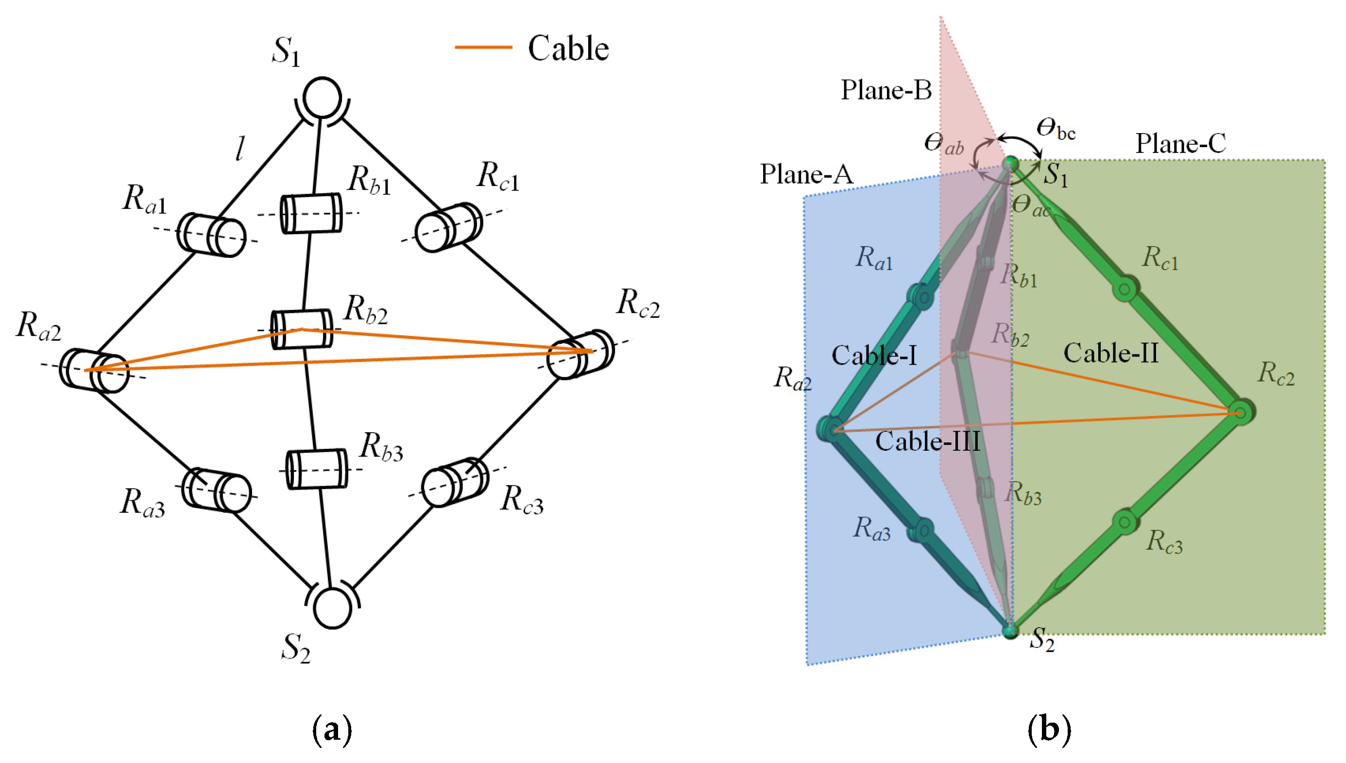
According to the kinematics characteristics of the flexible joint, it can be simplified as a spherical pair. The schematic diagram of the simplified mechanism and the 3D model are shown in Figure 2a and Figure 2b, respectively.
After simplification, the rigid–flexible coupling rolling mechanism is composed of three SRRRS branched chains and three flexible cables. In Figure 2a, S1-Ra1-Ra2-Ra3-S2 is the branched chain A, including two spherical pairs (S1, S2) and three revolute pairs (Ra1, Ra2, Ra3). The axes of the three revolute pairs are parallel to each other, as indicated by the dashed lines in the figure, and are perpendicular to the plane A where the branched chain A is located. S1-Rb1-Rb2-Rb3-S2 is the branched chain B, including two spherical pairs (S1, S2) and three revolute pairs (Rb1, Rb2, Rb3). The axes of the three revolute pairs are parallel to each other and perpendicular to the plane B where the branched chain B is located. S1-Rc1-Rc2-Rc3-S2 is the branched chain C, including two spherical pairs (S1, S2) and three revolute pairs (Rc1, Rc2, Rc3). The axes of the three revolute pairs are parallel to each other and perpendicular to the plane C where the branched chain C is located. Three SRRRS branched chains are connected by two spherical pairs, S1 and S2. Cable I connects Ra2 and Rb2, Cable II connects Rb2 and Rc2, and Cable III connects Rc2 and Ra2. Cable I, Cable II and Cable III are connected end to end to form a closed loop, and the flexible cables form a closed loop with the branched chain, respectively, as shown in Figure 2b.

2.2. DOF Calculation of the Simplified Model

After simplification, the rigid–flexible coupling rolling mechanism is composed of two parts: the rigid linkage mechanism and flexible cables. Since the flexible cables can only bear one-way tension but cannot bear pressure, when the flexible cable is relaxed, the mechanism can be equivalent to a purely rigid linkage mechanism. Therefore, the DOF analysis method based on the assembly process was adopted to analyze the DOF of the simplified mechanism, and the G-K formula is used for verification. Then, the influence of the flexible cable on the movement of the mechanism is analyzed, and the influence of the elastic force generated by the elastic deformation of the flexible joint on the movement of the whole mechanism is analyzed.
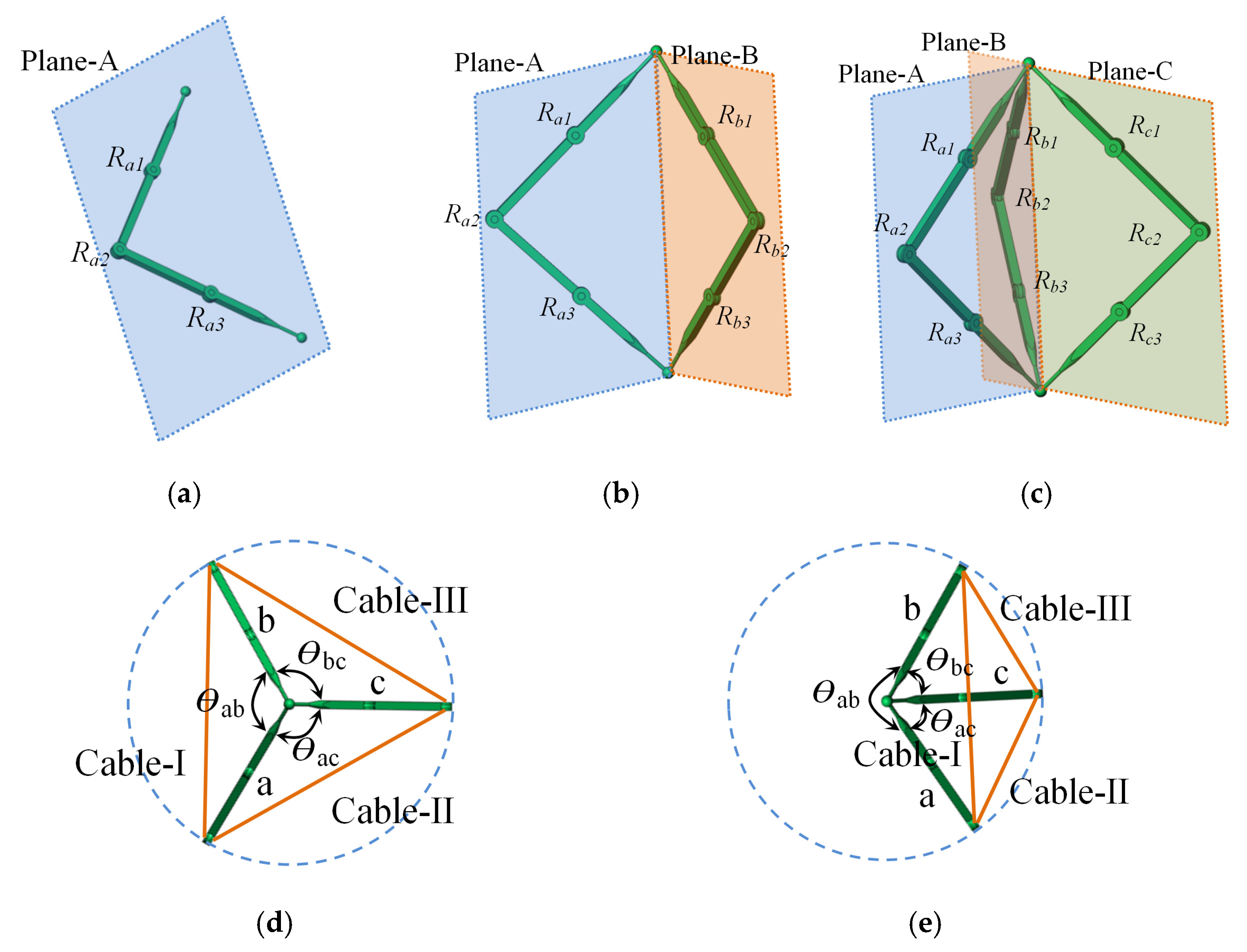
Firstly, the assembly of the branched chain A is completed, as shown in Figure 3a, and the DOF analysis of the branched chain A is carried out. Each rotation axis of the branched chain A is parallel and perpendicular to the same plane. The spherical pairs S1 and S2 are located at both ends of the branched chain A and do not participate in assembly, and the two spherical pairs have not been formed. Therefore, the branched chain A can be regarded as a planar 3R mechanism. The DOF Fa of the branched chain A is calculated according to Equation (1):
F a = 3 n 2 L =   3 × 3 2 × 3 = 3
where n is the number of active links in the branched chain A not including the frame and L is the number of lower pairs in the branched chain A. Fa is the DOF of the branched chain A.
The branched chain B is assembled on the basis of the branched chain A, as shown in Figure 3b. The branched chain B has the same structure as the branched chain A. Since the assembly of the branched chain A has been completed, the branched chain A can be regarded as a rigid body, and the positions of the spherical pairs S1 and S2 of the branched chain B are fixed in plane B; thus, the mechanism can be simplified as a closed-loop five-bar mechanism in plane B, S1 and S2 are regarded as revolute pairs in plane B, and the fifth bar is a simplified virtual bar of the branched chain A. The DOF Fb of the branched chain B in plane B can be obtained according to Equation (2):
F b = 3 n 2 L =   3 × 4 2 × 5 =   2
where n is the number of active links of the simplified mechanism in plane B not including the frame and L is the number of the lower pairs of the simplified mechanism in plane B.
The two spherical pairs S1 and S2 formed between the branched chain A and the branched chain B enable the two branched chains to have a relative rotational DOF. Therefore, the DOF Fab of the assembly of the branched chains A and B in the mechanism is obtained according to Equation (3):
F ab = F a + F b + 1 = 6
where Fa is the DOF of assembly of the branched chains A alone and Fb is the DOF in plane B after assembly of the branched chains A and B.
Finally, the branched chain C is assembled, as shown in Figure 3c. The assembly of the branched chain C is similar to that of the branched chain B. The assembled part of the mechanism is regarded as a rigid body and as the virtual fifth bar in plane C. S1 and S2 are regarded as the revolute pairs in plane C. The DOF of the simplified mechanism in plane C can be obtained according to Equation (4):
F c = 3 n 2 L = 3 × 4 2 × 5 = 2
where Fc is the DOF of the branched chain C in plane C, n is the number of active links of the simplified mechanism in plane C not including the frame, and L is the number of the lower pairs of the simplified mechanism in plane C.
Under the action of the two spherical pairs S1 and S2, there is a relative rotational DOF between the branched chain C and the assembled mechanism. The DOF F of the overall simplified mechanism is:
F = F ab + F c + 1 = 9
where Fab is the DOF of the mechanism with the branched chain A and the branched chain B assembled and Fc is the DOF in plane C after the assembly of the mechanism.
The G-K formula is used to verify the DOF of the simplified mechanism, as shown in Figure 2b. First, the DOF of the closed-loop mechanism formed by the branched chains A and B are calculated according to Equation (6):
F 1 = 6 ( n g 1 ) + i = 1 g f i = 6 ( 8 8 1 ) + 12 = 6
where F1 is the DOF of the closed-loop mechanism formed by the branched chain A and the branched chain B; n is the number of total links including the frame; g is the number of kinematic pairs; and fi is the number of DOF for the ith kinematic pair, i = 1 g f i = 12 .
The closed loop formed by the branched chain A and branched chain B is regarded as a rigid body, and it forms a closed loop with the branched chain C, using the G-K formula to obtain its DOF according to Equation (7):
F 2 = 6 ( n g 1 ) + i g f i = 6 ( 5 5 1 ) + 9 = 3
where F2 is the DOF of the mechanism formed with the branched chain C after the branched chain A and B are equivalent to a rigid body; n is the number of components including the frame; g is the number of kinematic pairs; and fi is the DOF of the kinematic pair, i = 1 g f i = 9 .
The overall DOF of the simplified mechanism can be obtained according to Equation (8):
F = F 1 + F 2 = 9
Therefore, the DOF of the simplified model of the rigid–flexible coupling rolling mechanism are nine.
For parallel mechanisms with closed-loop branch chains, the closed-loop chains should be equivalently regarded as generalized kinematic pairs with specific degree of freedom characteristics, thereby converting them into standard parallel mechanism forms and conducting degree of freedom analysis. The constrained screw system of the branch chain can be obtained through the kinematic screw system of the branch chain. The absence of a common constrained screw within the constrained screw systems of each branch chain confirms that the mechanism has no redundant constraints [31]. According to the idea of link demolishing and equivalent in reference [31], it can be demonstrated that the rigid–flexible coupled rolling mechanism proposed in this paper has no redundant constraints.
By analyzing the simplified model, we derived the degrees of freedom of the rigid mechanism, thereby eliminating the need for complex modeling and analysis of the mechanism’s flexible joints. However, its correctness still requires experimental verification. The selection of the prototype drive and parameter settings in the experiment were both based on the kinematics derived from the simplified model. During the experiment, the expected star rolling gait and deformable triangular prism rolling gait were observed, which proves that the results obtained by analyzing the mechanism with the simplified model are correct.

2.3. Influence of Flexible Cables and Flexible Joints

Cable I connects Ra2 and Rb2 to form a closed loop with the branched chains A and B and does not contact other components in the mechanism, as shown in Figure 1a. Due to the joint action of the two spherical pairs S1 and S2, the relative rotation around the center line of the two spherical pairs is formed between the branched chain A and the branched chain B, and the flexible cable can only bear the tension but not the pressure; thus, the function of Cable I on the mechanism is to reduce the angle θab between the plane of the branched chain A and the branched chain B. The function of Cable II and Cable III is similar to that of Cable I. The function of Cable II on the mechanism is to reduce the angle θac between the planes of the branched chain A and the branched chain C, and the function of Cable III on the mechanism is to reduce the angle θbc between the planes of the branched chain B and the branched chain C.
In the movement process of the rigid–flexible coupling rolling robot, the elastic deformation of the flexible joint results in the elastic force between the branched chains, which makes the angle between the planes of the branched chains tend to be 120°. The projection of the closed-loop structure formed by the flexible cable and the branched chain on the plane perpendicular to the rotation axis is shown in Figure 3d. The three planes located by the branched chain divide 360° around its relative rotation axis, and the size of the included angle is controlled by the contraction of the flexible cable. The angle relationship between the planes where the branched chains are located is as follows:
θ ab + θ bc + θ ac = 360 °
where θab is the angle between plane A and plane B; θac is the angle between plane A and plane C; and θbc is the angle between plane B and plane C.
When the angle between the planes of the branched chain is greater than 180°, the situation as shown in Figure 3e will appear. At this time, under the action of the elastic force generated by the elastic deformation of the triangular flexible joint, θab has a decreasing trend, which is limited by the length of the flexible cable.
Based on the above analysis, it can be seen that the triangular flexible joint and the flexible cable together determine the relative rotation positions between the planes of the three branched chains in the mechanism, the values of θab, θac, and θbc.
During the movement of the mechanism, in order to ensure that the torque generated by the elasticity of the flexible joint can bring the branched chain back to its initial position, the following conditions need to be met: when the flexible joint bends by π/3 rad, the torque it generates is sufficient to overcome the maximum torque caused by the weight of the single branched chain.
The fabricated flexible joint has an area of 157 mm2, an elastic modulus of 3 MPa, a length of 75 mm, and a cross-sectional moment of inertia of 6.08 × 10⁻⁹ m4. When bent by π/3 rad, the bending torque generated is 1.9 N∙m. Since there are two flexible joints, the generated bending torque can be 3.8 N∙m. Assuming the length of each link is l, the weight is 0.25 kg, and the number of single branched chain links is four; after calculation, the length of the link should be less than 506.67 mm. Considering that the appearance size of the servo motor used in the later prototype production is 40 mm × 40 mm × 20 mm, the length of the link should be greater than 80 mm. During the modeling process of the prototype, the length of the link should be between 80 mm and 506.67 mm.

2.4. Differences Between the Simplified Model and the Actual Model

According to the above analysis, the DOF of the simplified mechanism are nine, that is, in order to make the mechanism have a definite motion, a total of nine input parameters are needed: one of the three planar 3R branched chains needs three angle input parameters, the other two branched chains need two angle input parameters, respectively, and there need to be two angle input parameters between the three planes where the branched chain is located. However, in practice, the angles between the planes of the branched chains are determined by the length of the three flexible cables. Therefore, in practice, ten input parameters are required to make the rigid–flexible coupling rolling mechanism have a definite motion. One of the three planar 3R branched chains needs three angle input parameters, the other two branched chains need two angle input parameters, respectively, and there need to be three length input parameters of the three flexible cables.
The actual motion of the whole mechanism is driven by the data calculated by the simplified model; due to the elastic deformation of the flexible joint during the movement, it has a certain influence on the angle of the mechanism without driving the joint, further affects the CoM displacement in the rolling process of the mechanism, and increases the uncertainty in the motion process of the mechanism. In addition, the spherical joint approximation simplifies the kinematic modeling; it does not fully capture the distributed rotation center and configuration-dependent stiffness variations in the actual flexible triangular joint. In engineering design, in order to reduce this adverse effect, the flexible joints should be as small as possible while still meeting the requirements of strength. This is to prevent excessive deformation of the joints. Each joint in the branched chain is added with a drive motor. According to the above analysis, a total of 12 driving motors are needed for the mechanism, and the linear distance between the nodes connected to the flexible joints at both ends of the branched chain should be equal.

3. Kinematics Analysis of Two Rolling Modes

The design of the deformable triangular prism rolling gait and star-shaped rolling gait, based on the symmetry characteristics of the triangular prism and tetrahedron, helps enhance the stability of mobile robots. Simultaneously, this symmetry also simplifies the model, making the control process relatively simpler.
Two rolling modes are designed for this rigid–flexible coupling rolling mechanism: one is the star gait rolling mode, and the other is the deformable triangular prism rolling mode. To facilitate the description of the mechanism’s motion and ensure the rigor of the analysis, the following assumptions are made: the flexible cable has negligible mass, which is assumed to be zero during the motion of the mechanism. The cable is inextensible and perfectly flexible, with no resistance to bending. elastic deformation and associated internal stresses are neglected in the analysis; The link is modeled as a rigid body that does not deform during motion. For dynamic analysis, its mass is assumed to be concentrated equally at the two end joints; the assumption regarding flexible joints is the same as that in Section 2 of this paper.

3.1. Star Gait Rolling Mode

3.1.1. Star Gait Rolling Process

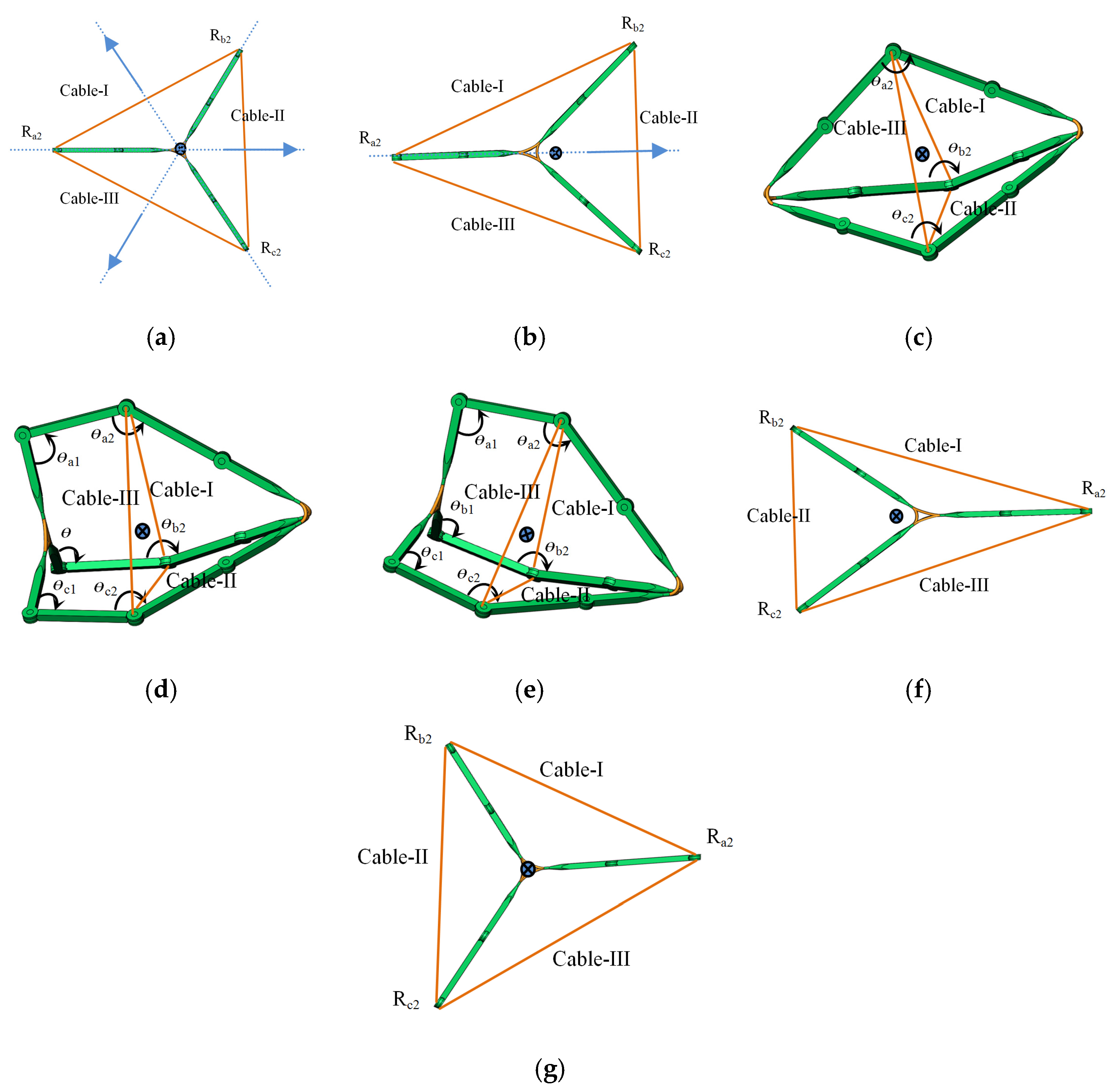
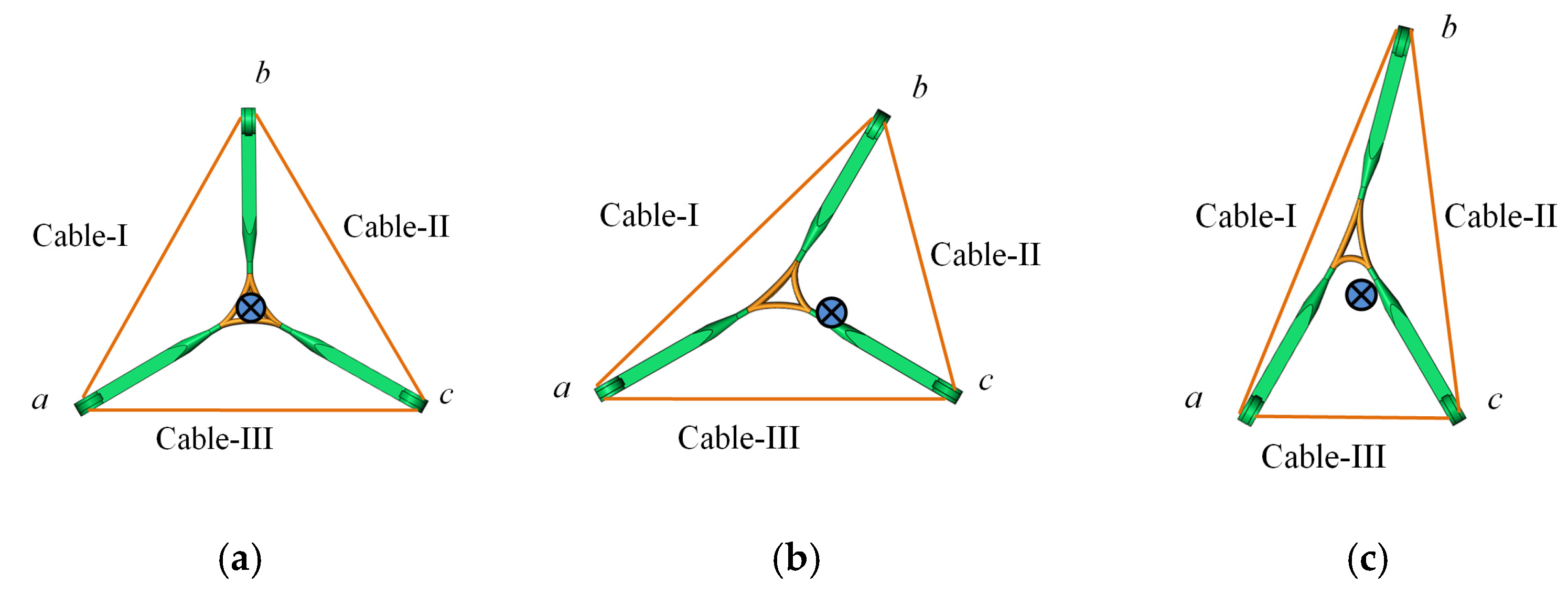
During the motion in star gait rolling mode, the mechanism is always symmetric with respect to the middle plane perpendicular to the ground in the forward direction, as shown in Figure 4c.The flexible cable mainly plays the role of direction adjustment, and the drive of the revolute joint is mainly used as the main drive in the rolling process of the mechanism. Taking the length of the rigid link in the mechanism as l and the input parameter θ = [θa1, θa2, θa3, θb1, θb2, θb3, θc1, θc2, θc3], lCable = [lI, lII, lIII], the specific rolling process is as follows:
a. The initial state of the mechanism is shown in Figure 4a, with three alternative directions of movement. The mechanism is in a contracting state, an equilateral triangle, and the center of gravity is located at the center of the shape. θa1 = θa3 = θb1 = θb3 = θc1 = θc3 = π, θa2 = θb2 = θc2 = 0, lI = lII = lIII = 2 3 l.
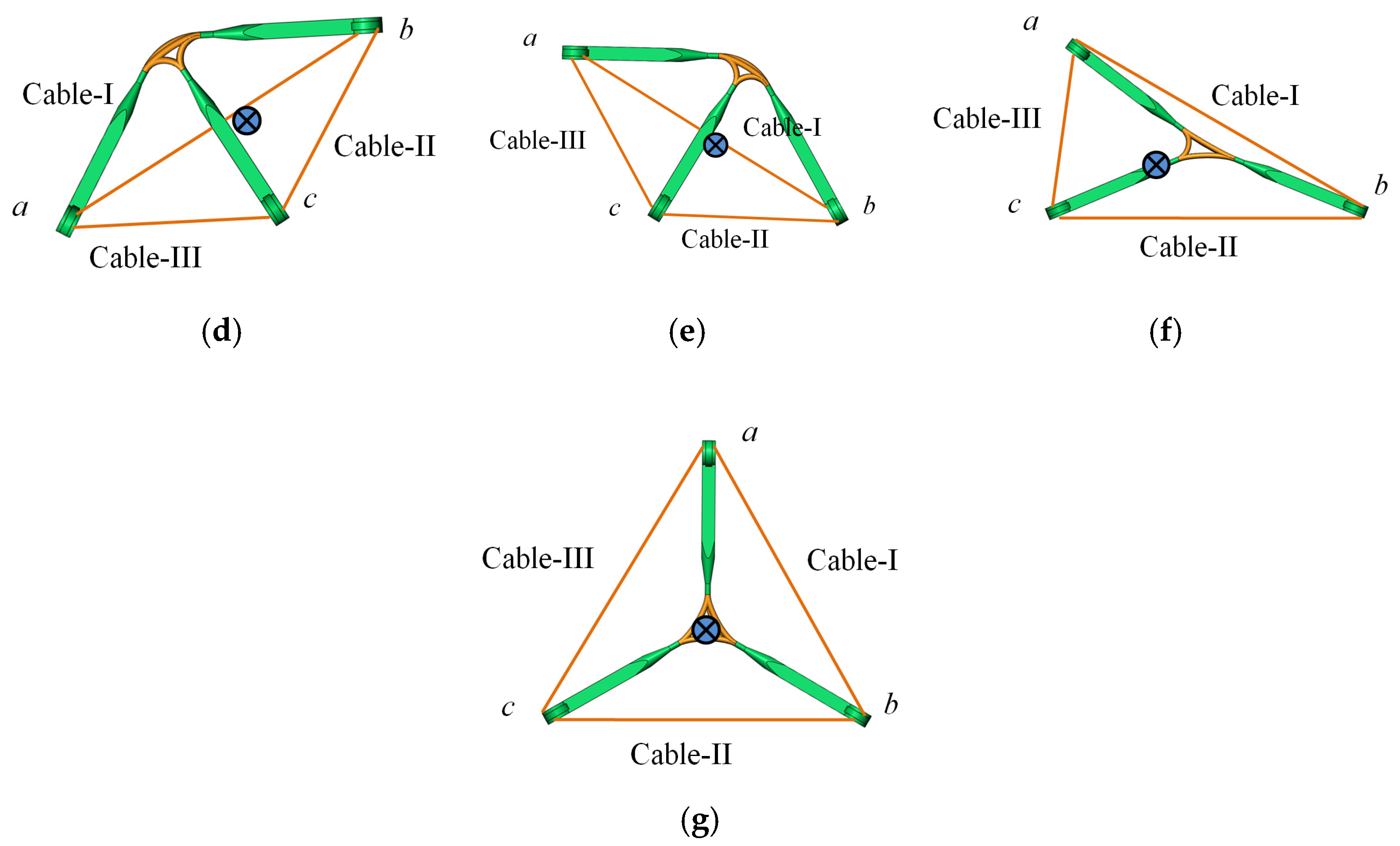
b. Cable II contracts to lII = 2l, Cable I and Cable III are pulled and elongated, and the center of gravity of the mechanism moves to the triangular area formed by Cable II, the branched chain B and the branched chain C, as shown in Figure 4b.
c. [θa2, θb2, θc2] expand at the same angular velocity, while lI and lIII are contracting at the same rate. The mechanism is extended and always symmetric about the middle plane, while the other input parameters remain unchanged. At this point, the supporting region of the mechanism is a triangular region formed by Cable II, the branched chain B and the branched chain C, and the CoM moves toward Cable II, the boundary of the supporting region, as shown in Figure 4c.
d. When the lengths of the cables are lI = lII = lIII = 2l, the geometrical outer surfaces of the mechanism are all equilateral triangles. The CoM of the mechanism is located at the center of the equilateral triangle formed by the flexible cable. [θa1, θb1, θc1] decrease so that the CoM of the mechanism exceeds the boundary of the support area, the Cable II, making the mechanism roll around Cable II, as shown in Figure 4d,e.
e. [θa2, θb2, θc2] decrease to 0 with equal angular velocity. [θa1, θb1, θc1] increase to π with equal angular velocity. The mechanism changes from Figure 4e,f.
f. lI and lIII shrink to 2 3 l at the same speed, the mechanism returns to the initial state, and a rolling period ends.
When the length of Cable II is 0, branches B and C are completely parallel and in contact with each other. At this point, the minimum width that can be passed through is 2lW, where lW is the width of the link. At this time, the stability of this rolling mechanism is poor because the width of the supporting area formed by the link is the narrowest.
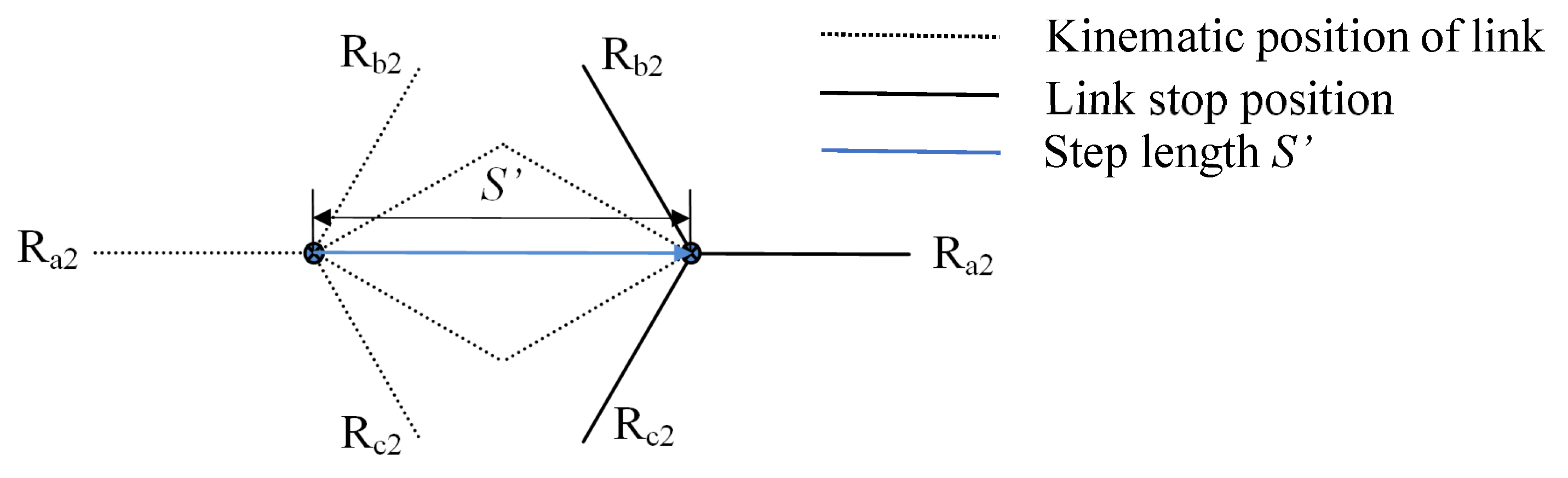
When the rigid–flexible coupling rolling mechanism is restored to the initial state each time, the rolling direction can be reselected, and the rolling direction is the angular bisector of the angle between the planes where the branched chains are located. The rolling step length is shown in Figure 5. The rolling step length can be obtained according to Equation (10):
S = 2 ( 2 l ) 2 l II 2 2
where S′ is the rolling step length with star gait; l is the length of the rigid link; and lII is the length of Cable II.

3.1.2. Inverse Kinematics in Star Gait Rolling Mode

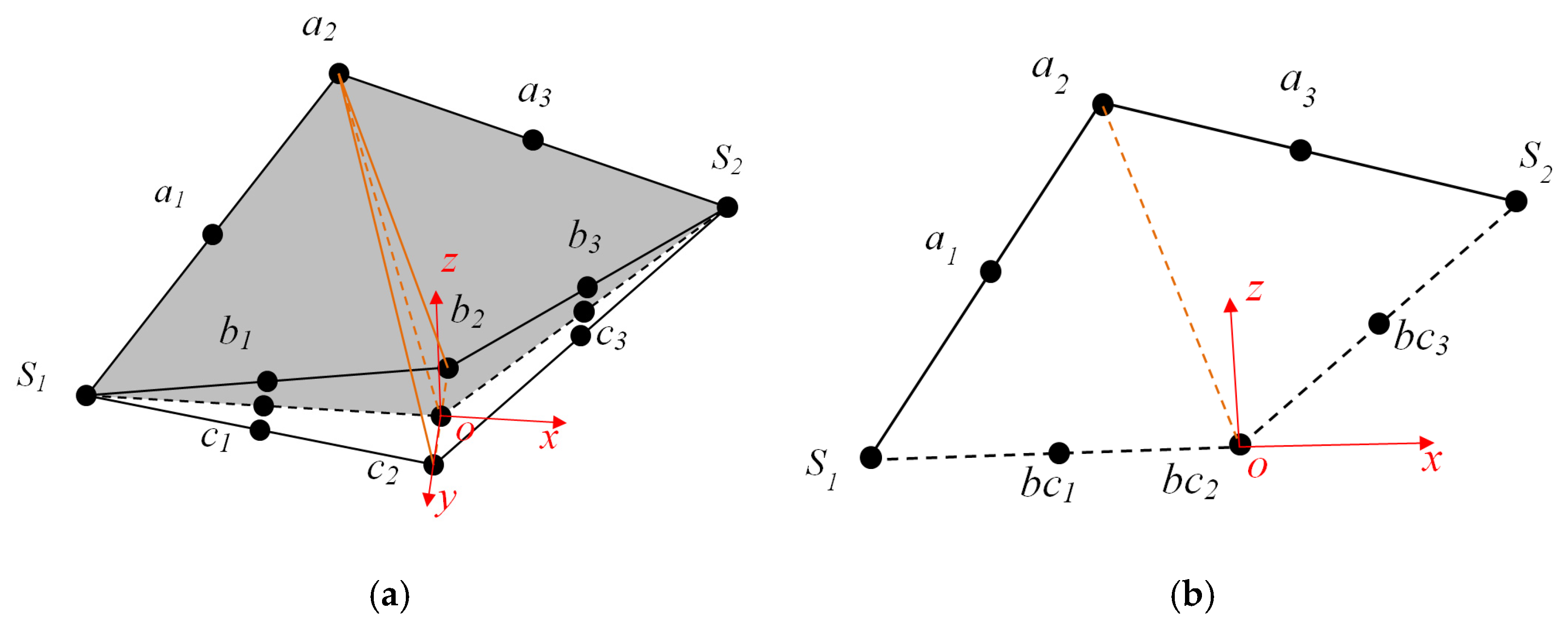
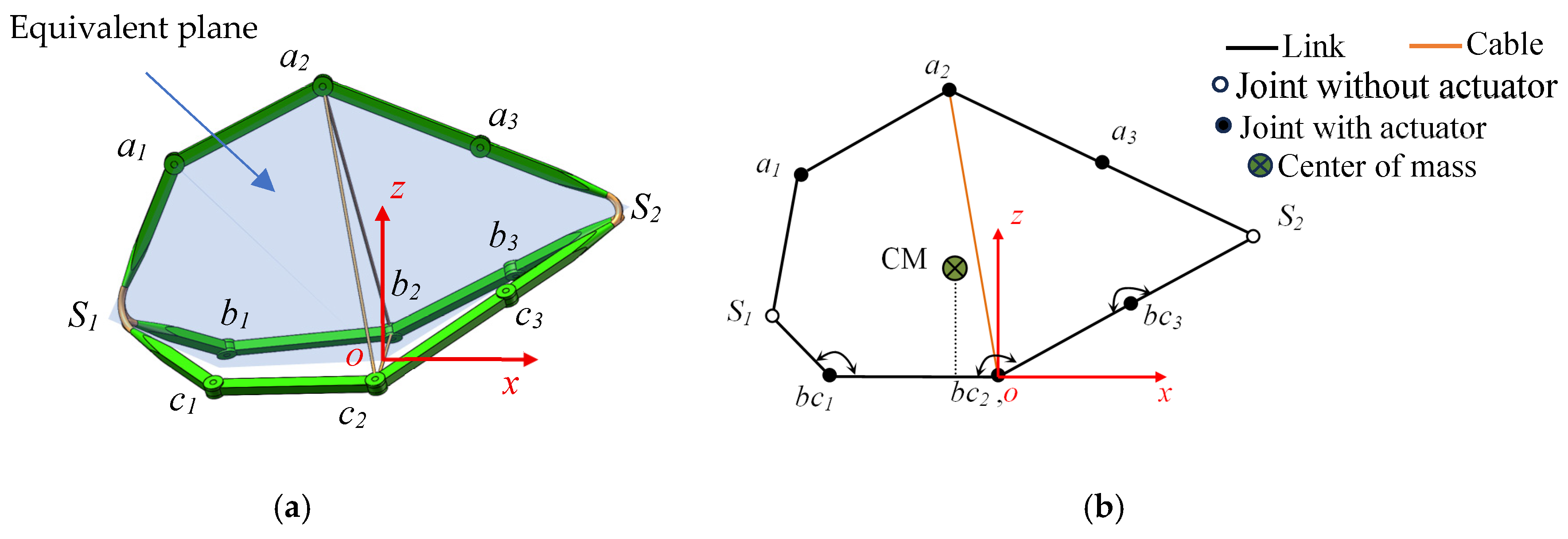
According to the mechanism in star gait rolling mode, always stay on the characteristics of the middle plane of symmetry, and the effect of the flexible cable is to keep the mechanisms about the middle plane of symmetry, with revolute pair s as the main drive of rolling motion; thus, the theory of equivalent planar mechanism analysis is used to simplify the process of theoretical analysis of this coupled rolling mechanism. This equivalent two-dimensional planar mechanism is an eight-bar mechanism with variable link length, as shown in Figure 6a,b. The support area is formed by part of the links in two branched chains, and projection is a linear segment of variable length. From the rolling process, it can be seen that the CoM of the mechanism is successively from the variable length links S1bc1, bc1 bc2, bc2 bc3, bc3S2 passes over it.
As shown in Figure 6a, the x-axis is the forward direction of the mechanism, origin O is located at the midpoint of Cable II, z-axis is vertical to the ground, and y-axis coincides with Cable II, of which the direction is determined by the right-hand rule.
The rotary drive located at c1 and b1 drives at the same speed and direction as θc1 and θb1. The line between c1 and b1 is parallel to the y-axis, and the projection is bc1 point. The two revolute joints (Rc1, Rb1) are equivalent to one revolute joint (Rbc1), as shown in Figure 6b. Similarly, the equivalent revolute joints Rbc2 and Rbc3 can be obtained. The equivalent planar eight-bar mechanism is obtained in the o-xz plane. The initial state of the mechanism has three symmetric planes and three rolling directions that can be selected. The following analysis is based on the motion state in Figure 6b.
In the equivalent two-dimensional planar mechanism, the configuration of the equivalent planar eight-bar mechanism can be defined by the connections between joints and linkages and joint positions; thus, the connectivity in the mechanism can be mathematically modeled as a graphic reference [32]: Gmodel = (J, L), L = [LS1bc1, L bc1bc2, L bc2bc3, Lbc2s2, LS2a3, La3a2, La2a1, La1S1] stands for equivalent linkage, and A link Lk = [Ji, Jj] represents the connection of the joints at both ends of the equivalent link. The position of the revolute joint Ji is represented by PJ= [PJx, PJy]T. All joint positions are represented by
x1= [PS1x, Pbc1x, Pbc2x, Pbc3x, PS2x, Pa1x, Pa2x, Pa3x, PS1y, Pbc1y, Pbc2y, Pbc3y, PS2y, Pa1y, Pa2y, Pa3y]
Taking all the lengths of rigid links in the mechanism as l, during rolling input parameter θ = [θa1, θa2, θa3, θb1, θb2, θb3, θc1, θc2, θc3]. lCable = [lI, lII, lIII].
The distance between the revolute joints is lk1.
l k 1 = P J P J
where   is 2 norm, and it can be used to represent the distance between two revolute pair s in planar mechanism. In the equivalent mechanism of star gait rolling mode, lk1 is the distance between the revolute joints; PJ and PJ represent the node positions at both ends of the equivalent link.
l k 1 = L s 1 a 2 L a 1 a 3 L a 2 s 2 L s 1 s 2 L s 1 b c 2 L b c 2 s 2 = 2 l sin θ a 1 2 2 l sin θ a 2 2 2 l sin θ a 3 2 2 l sin θ c 2 2 2 ( 2 l sin θ c 1 2 ) 2 ( l I I 2 ) 2 ( 2 l sin θ 3 2 ) 2 ( l I I 2 ) 2
The relation between the angular velocity of the driver θ ˙ and the node velocity P J ˙ can be obtained by taking the derivative of the Equation (12).
  l cos θ a 1 2 θ a 1 ˙ l cos θ a 2 2 θ a 2 ˙ l cos θ a 3 2 θ a 3 ˙ 2 l cos θ c 2 2 θ c 2 ˙ ( 2 l sin θ c 1 2 ) 2 ( l I I 2 ) 2 1 2 l sin θ c 1 2 cos θ c 1 2 θ c 1 ˙ ( 2 l sin θ c 3 2 ) 2 ( l I I 2 ) 2 1 2 l sin θ c 3 2 cos θ c 3 2 θ c 3 ˙ = L ˙ S 1 a 2 L ˙ a 1 a 3 L ˙ a 2 s 2 L ˙ s 1 s 2 L ˙ s 1 bc 2 L ˙ bc 2 s 2 = P S 1 P a 2 T P S 1 ˙ + P a 2 P S 1 T P a 2 ˙ L S 1 a 2 P a 1 P a 3 T P a 1 ˙ + P a 3 P a 1 T P a 3 ˙ L a 1 a 3 P a 2 P S 2 T P a 2 ˙ + P a 2 P S 2 T P S 2 ˙ L a 2 S 2 P S 1 P S 2 T P S 1 ˙ + P S 2 P S 1 T P S 2 ˙ L S 1 S 2 P S 1 P b c 2 T P S 1 ˙ + P b c 2 P S 1 T P b c 2 ˙ L S 1 b c 2 P b c 2 P S 2 T P b c 2 ˙ + P S 2 P b c 2 T P S 2 ˙ L b c 2 S 2
The relation between the angular velocity θ ˙ and the node velocity P J ˙ is converted into matrix form
θ ˙ = R x 1 ˙
θ ˙ is the angular velocity matrix of the equivalent planar mechanism; R is the transformation matrix; x 1 ˙ is the node position velocity matrix.
  • where R can be obtained from Equation (13).

3.2. Motion Mode of the Deformable Triangular Prism

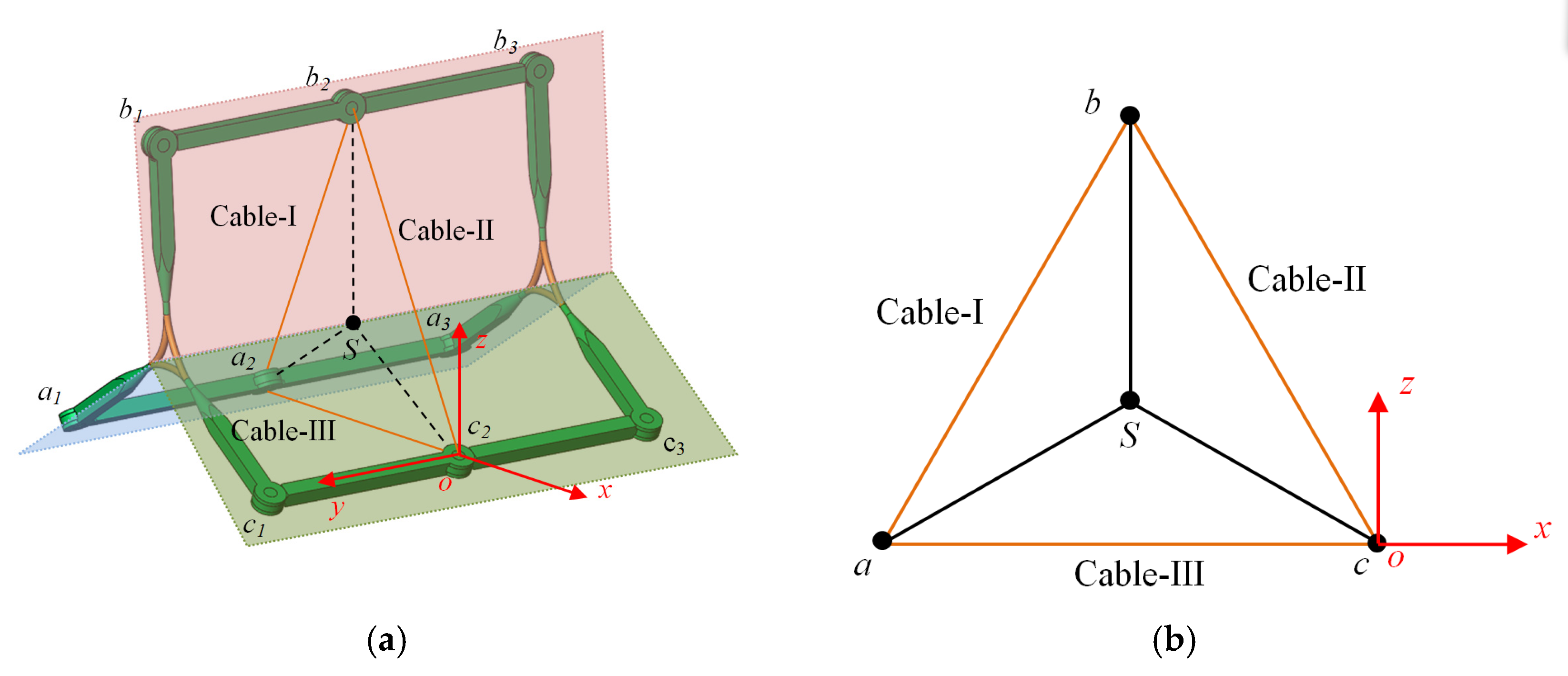
In the rolling process of this mode, the actuator controls the change in the length of the cable to control the forward rolling of the mechanism. When the flexible cable driving mechanism moves, the angles between all rigid links remain fixed, and there are only three variable input parameters, lCable = [lI, lII, lIII]. The rolling process is shown in Figure 7.

3.2.1. Motion Process of the Deformable Triangular Prism

The initial state of the rolling mode of the deformable triangular prism is shown in Figure 8a, θa1 = θb1 = θc1 = π/2, θa3 = θb3 = θc3 = π/2, θa2 = θb2 = θc2 = π. The mechanism moves forward through the contraction motion of three flexible cables, and the specific movement process is as follows:
a. Firstly, Cable II contracts, Cable I elongates, and Cable III remains unchanged. The CoM shifts to the boundary c of the support area, as shown in Figure 8b.
b. As the CoM is closer to the boundary of the support area at c, the maximum friction between c and the ground is greater than that between a and the ground, so the branched chain a moves closer to the branched chain C and the support area decreases, as shown in Figure 8c.
c. The contraction of Cable II makes the CoM of the mechanism exceed the boundary c of the support area, and the mechanism rolls around the boundary c of the support area, forming a new support area cb, as shown in Figure 8d,e.
d. When Cable II and Cable I extend, under the action of gravity and elastic force of the flexible joint, the included angle between the branched chain A and the branched chain C increases, the support area becomes larger, and the CoM of the mechanism moves further forward, as shown in Figure 8f.
e. Cable I contracts, Cable II stretches, and the mechanism is restored to the initial state, as shown in Figure 8g.
When the mechanism needs to turn, the equiangular velocity of the revolute joint drive θa1 = θb1 = θc1 or θa3 = θb3 = θc3 decreases, and the mechanism deforms into a triangular platform. Since the radius of the outer circle of the two bottom triangles is not equal, the mechanism will rotate around the virtual end point of the triangular platform during rolling. The rolling process driven by the flexible cable is similar to that shown in Figure 8.

3.2.2. Inverse Kinematics of the Deformable Triangular Prism

In rolling mode of the deformable triangular prism, the rigid–flexible coupling rolling mechanism keeps θa1 = θb1 = θc1 = π/2, θa3 = θb3 = θc3 = π/2, θa2 = θb2 = θc2 = π, moves forward through the contraction motion of three flexible cables, and is always symmetric about the o-xz plane, as shown in Figure 7a.
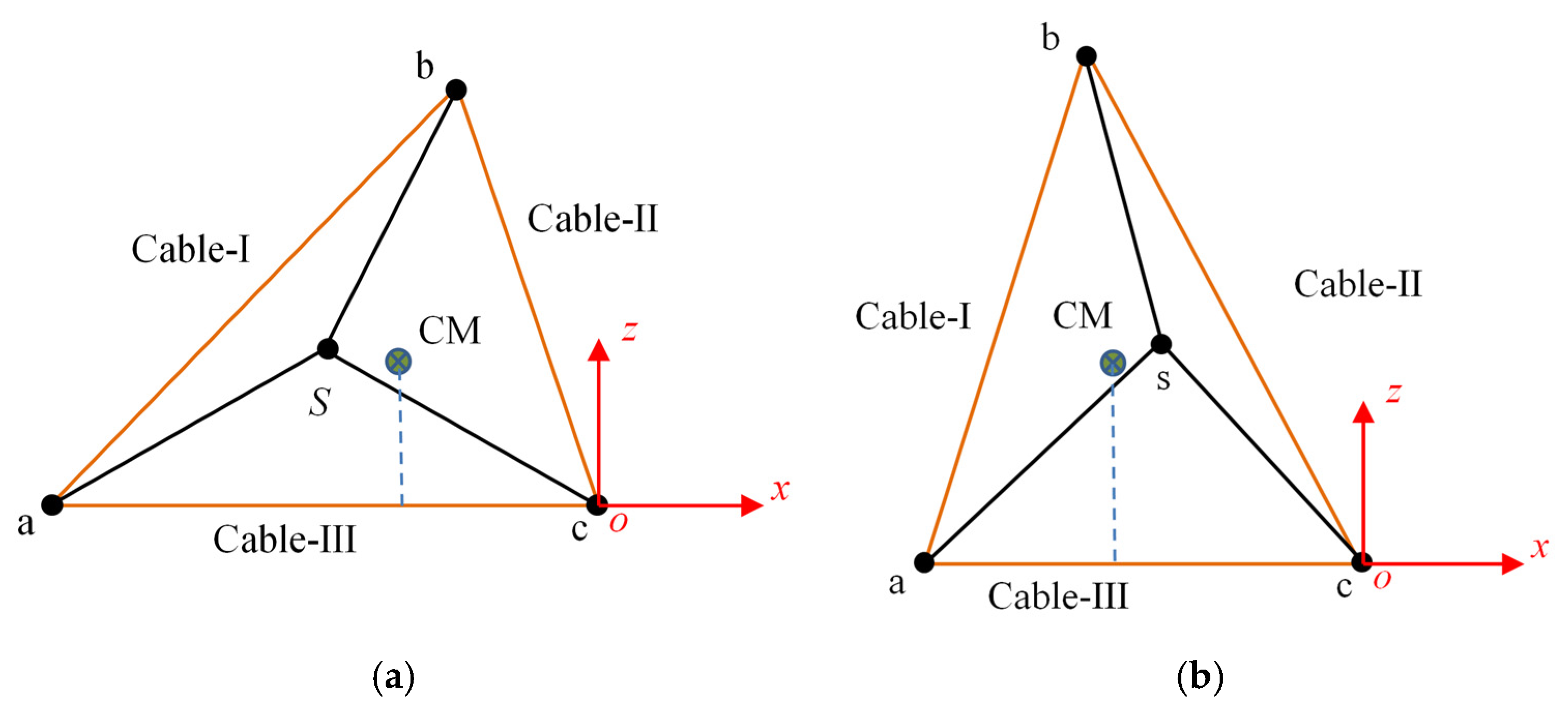
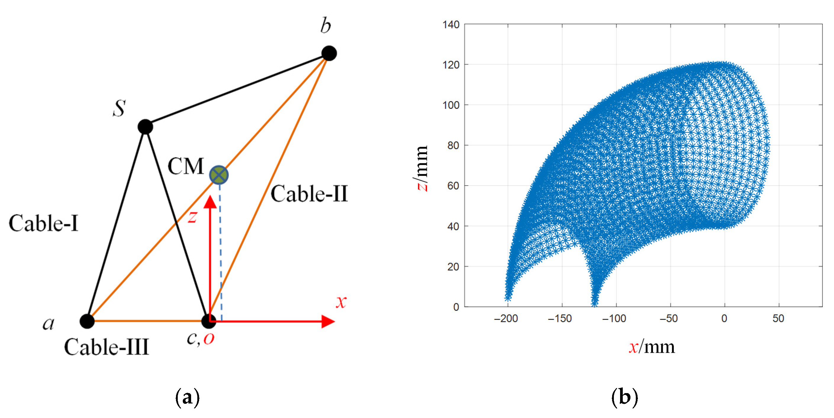
The projection of this mechanism on the o-xz plane is shown in Figure 7b. The support area is line segment ac, the projection of the three branched chains revolves around the projection point S of the flexible joint under the drive of the flexible cables, the projection of the branched chain A is aS, the projection of the branched chain B is bS, and the projection of the branched chain C is cS. A mathematical model was established for the equivalent planar mechanism. The node coordinates were expressed as pm = [pmx, pmy], m = [a, b, c, s], and the node positions were expressed as x2 = [pax, pay, pbx, pby, pcx, pcy, psx, psy], lCable = [lI, lII, lIII].
Lmm’ is the distance between nodes.
L mm = | | p m p m | |
In the equivalent mechanism of motion mode of the deformable triangular prism, Lmm is the distance between the revolute joints; Pm and Pm represent the node positions at both ends of the equivalent link.
In the process of motion, node position, input parameters, and the cable length lCable = [lI, lII, lIII] have the following relationship:
l I l II l III = L a b L b c L a c = | | p a p b | | | | p b p c | | | | p a p c | |
By taking the derivative of Equation (16), we can get the relationship between the change velocity of cable length and the node velocity.
l I ˙ l II ˙ l III ˙ = L a b ˙ L b c ˙ L a c ˙ = p a p b T p a ˙ + p b p a T p b ˙ l I p b p c T p b ˙ + p c p b T p c ˙ l II p a p c T p a ˙ + p c p a T p c ˙ l III
Converting Equation (17) into matrix form yields
l ˙ C a b l e = R 2 x 2 ˙
l ˙ C a b l e is the cable velocity matrix of the equivalent planar mechanism; R2 is the transformation matrix; x 2 ˙ is the node position velocity matrix.
  • where R2 can be obtained from Equation (17).

4. Gait Planning

During the rolling process of the rigid–flexible coupling rolling mechanism, there is an error between the actual displacement trajectory and the ideal displacement trajectory, which is mainly caused by the collision between the mechanism and the ground during rolling. The cause of collision is that the gravitational potential energy is converted into the dynamic potential energy of the mechanism when the mechanism overturns and changes the supporting area, and the collision between the mechanism and the ground cancels out part of the dynamic potential energy of the mechanism itself. When the mechanism overturns, the smaller the displacement of the CoM in the direction of gravity is, the smaller the dynamic potential energy converted from gravitational potential energy will be, and the smaller the collision degree between the mechanism and the ground will be, thus reducing the displacement error. According to this theory, the gait planning of the two rolling modes of the mechanism was carried out, and the collision rolling gait with the minimum impact was designed.

4.1. Collision Rolling Gait with Minimum Impact

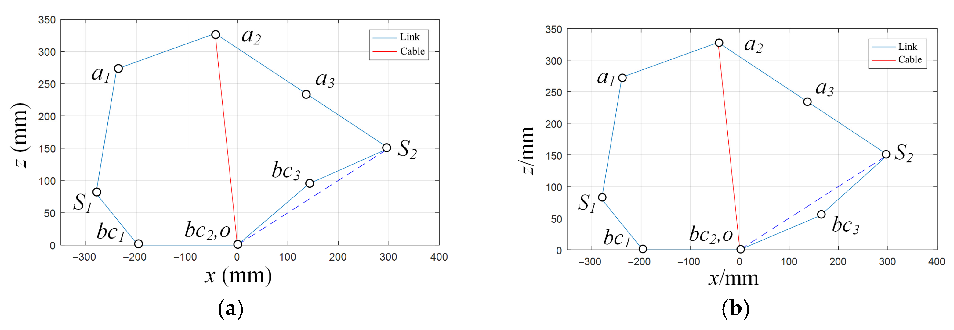
A complete motion period of the mechanism in star gait rolling mode is shown in Figure 4. The support area of the mechanism is formed by the branched chains C and B, and the CoM projection passes over the links S1bc1, bc1 bc2, bc2 bc3, bc1 bc2 in the equivalent planar mechanism in turn. Among them, S1 and S2 are the projections of the flexible joints; bc1 is the equivalent joint where the projections of b1 joint and c1 joint overlap; bc2 is the equivalent joint where the projections of b2 joint and c2 joint overlap; bc3 is the equivalent joint where the projections of b3 joint and c3 joint overlap; a1 is the projection of joint a1; a2 is the projection of joint a2; a3 is the projection of joint a3. The overturning process of this rigid–flexible coupling rolling mechanism is shown in Figure 4d,e. The mechanism adjusts the angle between the rigid links through the rotary actuators located on each revolute joint in the branched chain and then moves the CoM of the mechanism. The main function of the flexible cable is to maintain the symmetry of the mechanism on the o-xz plane. The equivalent planar mechanism diagram before the mechanism overturns is shown in Figure 9.
Because star gait rolling is a quasi-static process, the key to accomplishing this rolling gait is to make the projection of the CoM of the mechanism go beyond the supporting area, x C M > 0 . The mass of the rigid link is uniformly distributed at both ends of the rigid link, that is, the mass of the mechanism is distributed at each vertex of the equivalent planar mechanism, the CoM projection is CM, and the overturning condition of the mechanism is x C M > 0 , as shown in Figure 9. According to Equation (19) and the mass and position of each link, the coordinate rCM of the CoM can be obtained:
r C M = J m J P J J m J
where rCM represents the centroid position; mJ represents equivalent mass at the joint J; and PJ represents the position of the joint J.
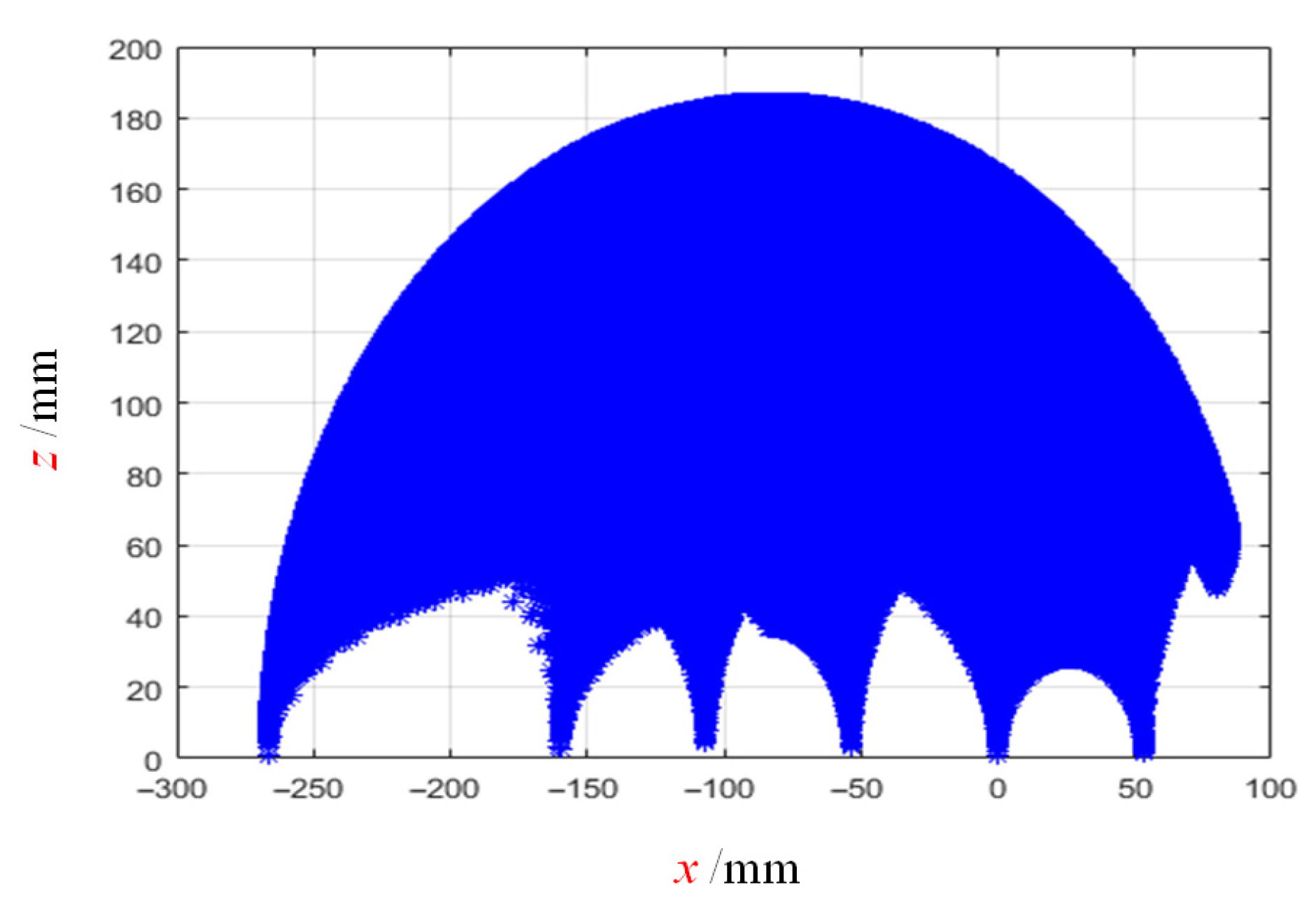
Assuming that the link projection bc1bc2 is always in contact with the ground, bc2 coincides with the origin o, according to Equation (19), and the projection of the CoM workspace of the rigid–flexible coupling rolling mechanism on the o-xz plane in star gait rolling mode can be obtained, as shown in Figure 10. The CoM workspace of this mechanism is continuous, and there is a projection region with the x-coordinate greater than 0, which indicates that this mechanism has the capability of rolling motion in star gait rolling mode.
Taking the length of the rigid link in the mechanism l = 160 mm, after the adjustment of the direction of the mechanism, the length of Cable II should always be kept at lII = 320 mm. The overall mass of the mechanism is set as mT = 3 kg, and the mass of a single rigid link is 0.25 kg. The influence of the mass of the cable and the flexible joint on the motion state of the mechanism and the influence of the deformation of the flexible joint are ignored. The rigid–flexible coupling rolling mechanism collides with the ground in two cases: the first is the collision between joint S2 and the ground, as shown in Figure 11a, and the second is the collision between equivalent joint bc3 and the ground, as shown in Figure 11b.
In the first case, when lI = lII = lIII = 320 mm, θa1 = θb1 = θc1 = 1.63 rad, θa2 = θb2 = θc2 = 2.36 rad, θa3 = θb3 = θc3 = π, we can obtain xCM = 2.2875 mm according to Equation (19). At this point, the mechanism will overturn around the equivalent joint bc2 and the point S2 where it collided with the ground, as shown in Figure 11a. According to Equation (20), the moment of inertia of the mechanism around the equivalent joint bc2 in this state can be obtained:
J z i = J m J p J 2
where J z i is the moment of inertia of the joint J.
According to Equation (21), the collision impulse I can obtain collision impulse I:
J z i ω 2 + J z i ω 1 = I l O J
where lOJ is the distance between the rotation point O ( point bc2 ) and the collision point J (point bc or S2), Jz1 = 0.1160 kg·m2, ω 1 and ω 2 are the angular velocities before and after the collision, and they satisfy the following relationship:
e = ω 2 ω 1
The recovery coefficient e = 0.4 based on the impact between the engineering plastic and the ground can be obtained by the following equation and take θ = [π/2, 0]:
1 2 J z 1 ω 1 2 = m T g l O C M 1 sin θ
where lOCM is the distance from the point of rotation to the CoM.
When S2 collides with the ground, the components of the impact impulse along the x-axis and z-axis received by point O (point bc2) are Iox1 = 2337.9 kg·mm/s, Ioz1 = −1040.9 kg·mm/s, respectively.
In the second case, let lI = lII = lIII = 320 mm, θa1 = θb1 = θc1 = 1.63 rad, θa2 = θb2 = θc2 = 2.36 rad, θa3 = π, θb3 = θc3 = 3.23 rad. According to Equation (19), we can obtain xCM = 2.2903 mm, and according to Equation (21), Jz2 = 119,200 kg mm2 can be obtained. Then, it can be concluded that the impulse component along the x-axis is Iox2 = 2327.6 kg·mm/s, and the impulse component along the y-axis is Ioz2 = −2096.5 kg·mm/s.
Compared with the collision process in the two cases, the impulse in the direction of the x-axis of the mechanism is similar, and Ioz1 decreases by 49.65% compared with Ioz2. In the rolling process, due to the limitation of joint working angle, the inevitable collision caused by the selection of configuration 1 can effectively reduce the collision impact.
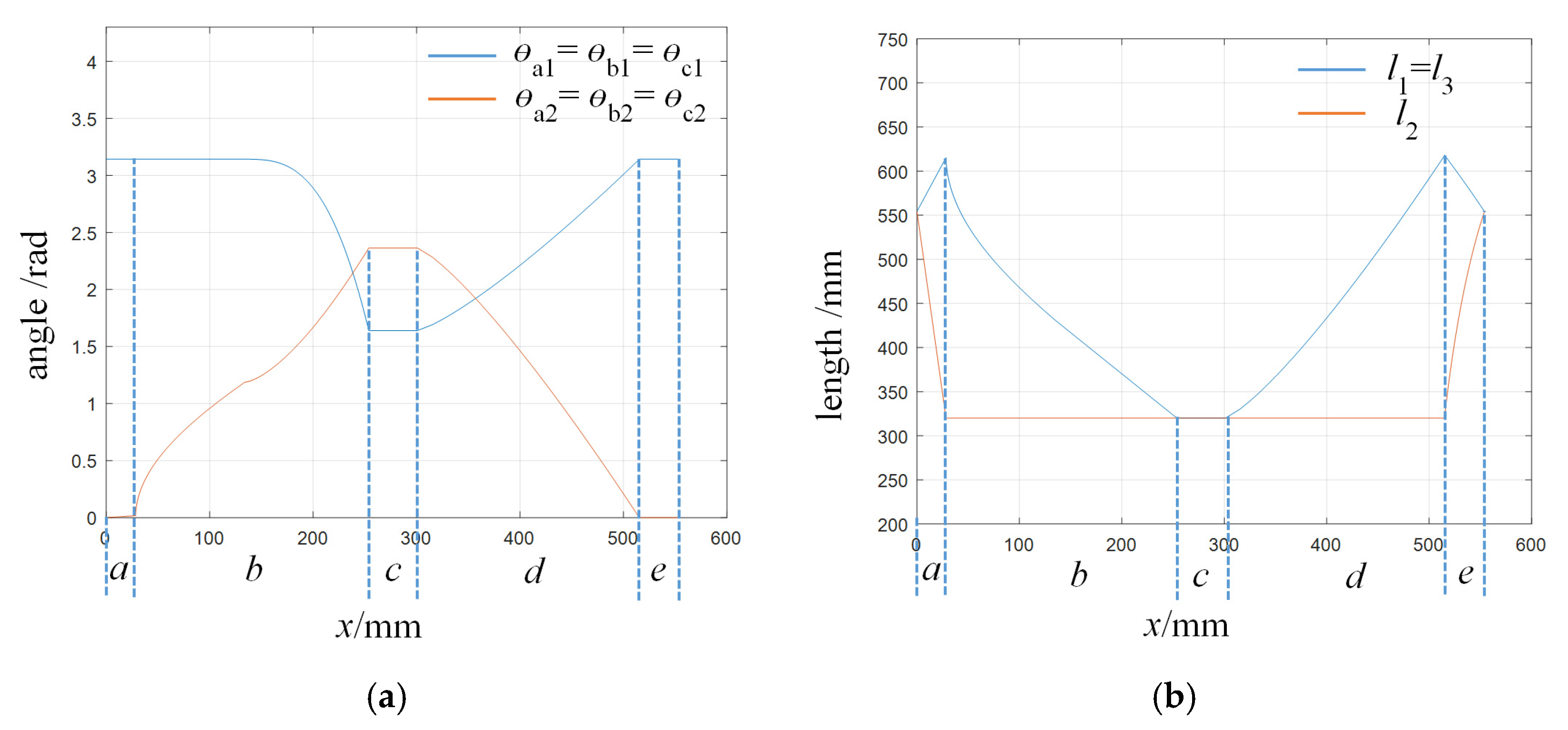
The projection of the supporting area is bc1bc2; in the case of configuration-1, the step size of the mechanism in a motion cycle is S′ = 320 3 mm; in order to simplify the control of the mechanism in the process of motion, take θa3 = θb3 = θc3 = π, θa1 = θb1 = θc1 = θ1 and θa2 = θb2 = θc1 = θ2. According to Equations (10) and (19), the relation between the displacement of the CoM in the x direction and the input variable can be obtained, as shown in Figure 11a,b. The variation in the rotational angle of the joint during the rolling process is shown in Figure 12a, and the variation in the length of the cable is shown in Figure 12b.The rolling process is as follows:
a. In the direction adjustment stage, Cable II shrinks to 320 mm, Cable I and Cable III elongate, and the angle between the links remains unchanged.
b. Control rolling stage 1. θ1 and θ2 change to drive the CoM movement; the rolling process is completely controllable.
c. In the rolling stage, as the change in θ1 and θ2 makes the CoM exceed the boundary of the support area, the mechanism will roll, and the rolling process is uncontrollable.
d. Control the rolling stage 2. After the mechanism rolls, a new support area is formed. θ1 and θ2 restore to the initial value and drive the CoM of the mechanism to move; the rolling process is completely controllable.
e. Each cable is restored to the initial state, and one rolling cycle is completed.

4.2. Two Motion Modes of the Deformable Triangular Prism

In the process of adopting rolling mode of the deformable triangular prism, there are two forms of movement: one is wriggling, and the other is rolling. The mechanism only depends on the change in the length of the three flexible cables to drive the mechanism to move; the joint angle is kept constant θa3 = θb3 = θc3 = π/2, θa1 = θb1 = θc1 = π/2, θa2 = θb2 = θc1 = π.

4.2.1. Creeping Motion Mode of the Deformable Triangular Prism

The creeping motion of the deformable triangular prism takes advantage of the difference between the maximum friction force generated by the two branched chains forming the support area and the ground. Under the action of the flexible cable, the distance between the ground contact points is extended or shortened, and then, the mechanism is driven forward.
In the movement process of the deformable triangular prism, the two branched chains contact the ground to form a support area, and the contact lengths of the two branched chains with the ground are both 2l, as shown in Figure 7a. The friction coefficient between the branched chain and the ground is f, the overall mass of the mechanism is mT, and the gravity coefficient is g. When the branched chain B deflects under the action of the flexible cable, the CoM of the mechanism is offset. Under the action of gravity, the branched chain A and branched chain C have the following relation with the maximum friction force that can be generated by the ground:
F a max = | | x C M p c x | | | | p c x p a x | | m T g f
where Famax represents the friction force between node a and the ground; xCM represents the centroid position; P represents the position of the relevant node; mT represents the weight of the entire mechanism; g is the coefficient of gravity; and f is the coefficient of friction.
F c max = | | x C M p a x | | | | p c x p a x | | m T g f
where Fcmax represents the friction force between node c and the ground; xCM represents the centroid position; P represents the position of the relevant node; mT represents the weight of the entire mechanism; g is the coefficient of gravity; and f is the coefficient of friction.
When the branched chain B rotates to the branched chain C under the action of the flexible cable, the CoM of the mechanism moves to the positive direction of x, as shown in Figure 13a. From the above equation, it can be known that Fcmax > Famax, and then, Cable III contracts, and since the two strands have different maximum friction with the ground, the contact point between the branched chain C and the ground remains unchanged, while the contact point between the branched chain A and the ground moves in the positive direction of the x-axis. When the mechanism is in the state as shown in Figure 13b, the branched chain B deflects toward the branched chain A under the action of the flexible cable, | | x C M p a x | | < | | x C M p c x | | ; according to Equations (24) and (25), we can obtain Fcmax < Famax. When Cable I and Cable II contract and Cable III stretches, since the maximum friction between the two chains and the ground is different, the contact point between the branched chain A and the ground remains unchanged, while the contact point between the branched chain C and the ground moves in the positive direction of the x-axis.
The creeping motion step length of this mechanism is adjustable, there are no collision and impact in the movement process, and the movement is accurate. However, due to the sliding friction with the ground all the time in the process of movement, the movement efficiency is reduced, and the movement can only be carried out on the flat ground, without the capability to overcome obstacles.

4.2.2. Rolling Motion Mode of the Deformable Triangular Prism

When the bottom cable contracts and the support area becomes smaller and the branched chain B deflects so that the CoM exceeds the support area, the mechanism will roll, as shown in Figure 14a.
Taking the length of the rigid link as l = 160 mm and the overall mass of the mechanism as mT = 3 kg, the mass of the rigid link of the mechanism is equivalent to both ends of the rigid link, and the mass of each point in the equivalent planar mechanism can be obtained, ms = ma = mb = mc = m′ = 0.75 kg. The CoM coordinates can be obtained according to Equation (19). The projection of the CoM workspace on the o-xz plane is shown in Figure 14b.
When the CoM coordinates are xCM > 0, the mechanism will roll; when the CoM coordinate is xCM = 0, the mechanism is in the critical state of rolling; when the CoM coordinates are xCM > 0, the mechanism can only move in creeping.
When rolling occurs, the maximum distance between point a and point c is the maximum width of the gully that can be crossed by the mechanism. In the equivalent planar mechanism, las = lsc = lsb = l = 160 mm, point c is coincident with the origin o, point a, point S, point c forms an isosceles triangle, psx = pax/2, pcx = 0, pax = −lII. According to Equation (19), we can get
x C M = p a x m a + p b x m b + p c x m c + p s x m s / m T
When xCM = 0, in order to maximize the lac, the rigid link sb should be kept horizontal according to the geometric relationship in the equivalent planar mechanism, that is, pbx = lSb + pax. According to Equation (26), lac = 80 mm can be obtained, that is, the mechanism can span an 80 mm gully at the maximum.
Compared with the creeping motion, the rolling motion of the deformable triangular prism improves the motion efficiency, which can not only cross gullies but also climb steps with a certain height, increasing the obstacle-crossing capability of the mechanism. However, there are collision and impact in the motion process, and the motion is not stable enough and the error is large.
The motion modes of the deformable triangular prism combine the advantages of creeping motion and rolling motion, which not only improves the motion efficiency of the mechanism but also increases obstacle-crossing capability, reduces motion error and improves motion accuracy.
When the mechanism needs to turn, making θa1 = θb1 = θc1 or θa3 = θb3 = θc3 decrease, the mechanism is deformed into a triangular platform. Since the radii of the circumference circles of the two bottom triangles is not equal, the mechanism will rotate around the virtual end point of the triangular platform during rolling.

5. Prototype Testing

A prototype was developed to verify the motion capability of the rigid–flexible coupling rolling mechanism, as shown in Figure 15. Nine servo motors to control the angle are installed at the nine revolute joints of the mechanism, and three motors to drive the flexible cable contraction are installed inside the three rigid links. The parameters of the prototype are given in Table 1. Combined with the kinematic derivation results, control the changes in joint angles and cable lengths to observe whether deformable star gait rolling and triangular prism rolling occur, verifying the correctness of the kinematics, degrees of freedom, and gait planning.
In the prototype, the control device of the cable is installed inside the link, the extension and retraction device of the cable is installed at one end of the cable, and the tensioning device of the cable is installed at the other end, which is used to keep the cable always under tension and maintain it in a tensioned state. The cable material is 0.5 mm steel wire; the material is 45# steel, with an elastic modulus of 210 GPa. The cable elongation deformation during the experiment can be considered as 0.
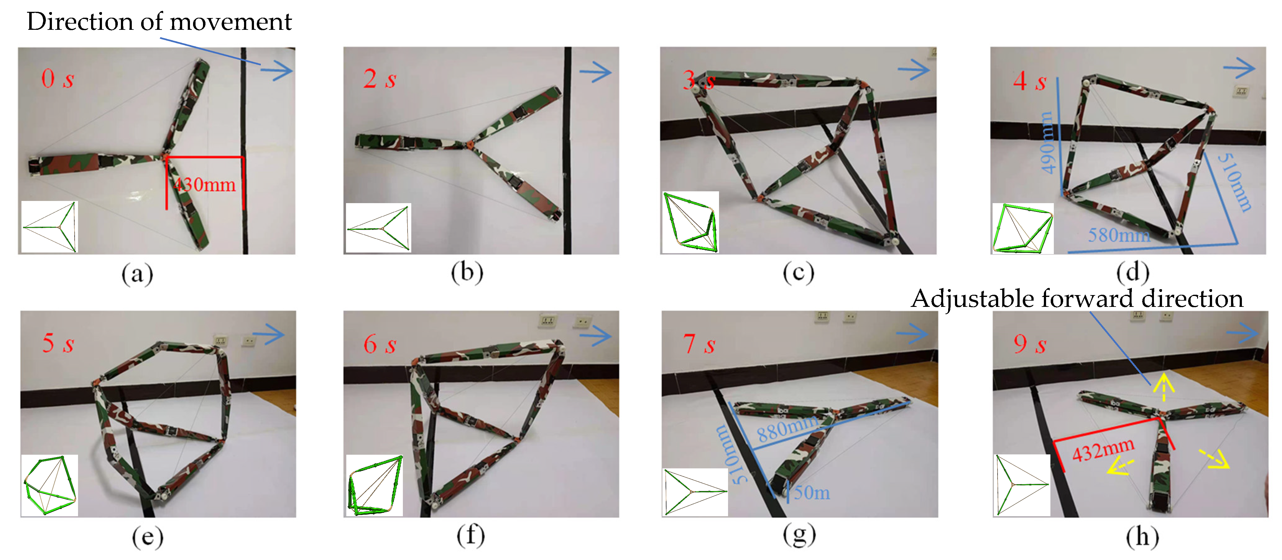
The initial state of the star gait rolling mode is: set the rolling step length to 866 mm. During the rolling process, first adjust the angle between the two chains in the forward direction to π/3. The initial lengths of the three cables are all 870 mm, the joint angle at the middle position in each chain is 0 rad, and the others are π, as Figure 16a. The length of the link is 250 mm, the width is 50 mm, and the minimum width it can pass through is 100 mm.
Figure 16 shows the motion process of the prototype in star gait rolling mode. A complete movement cycle is 9 s, and the step length is 862 mm, error: 4 mm (0.5%). After each rolling cycle, the mechanism will be restored to the initial state and can reselect the direction of movement, as shown in Figure 16h. In the process of motion, the maximum volume appears in Figure 16d, and the minimum volume appears in Figure 16g. In star gait rolling mode, the scaling ratio λ 1 of the mechanism can be obtained according to Equation (27), λ 1 = 6.46 .
λ = V max V min
λ is the scaling ratio of the mechanism during the movement process; Vmax is the maximum volume during the movement process; Vmin is the minimum volume during the movement process.
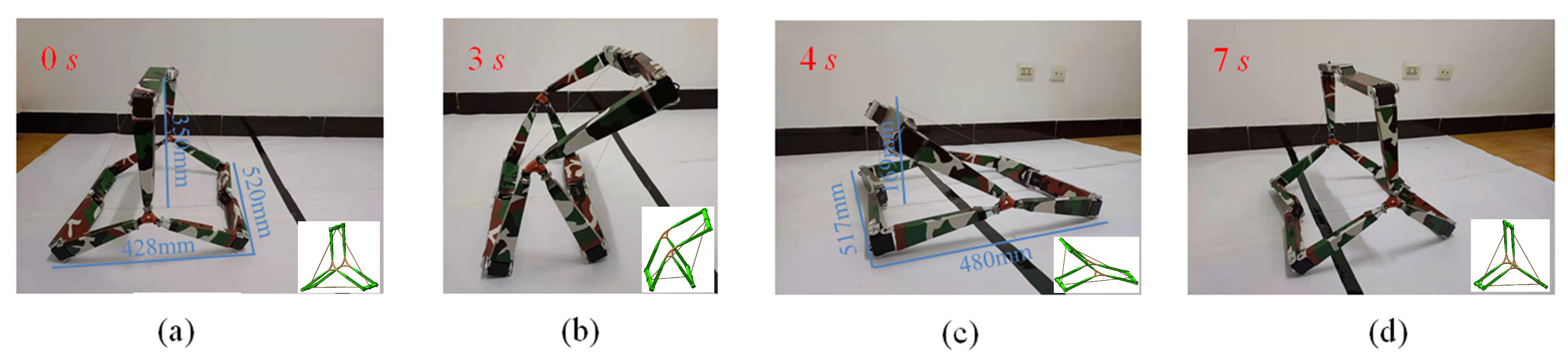
The initial state of the deformable triangular prism rolling mode is: set the rolling step length to 469.84 mm. Before the overturning, the angle between the two branches in the forward direction was 2.44 rad (140°); the initial lengths of the three cables are all 428 mm, the joint angle at the middle position in each chain is π, and the others are π/2, as Figure 17a.
In Figure 17, the mechanism moves forward in rolling mode of the deformable triangular prism by combining creeping motion and rolling motion, completes a roll within 7 s, and returns to the initial state, with a total movement of 480 mm, error: 10.06 mm (2.2%). In the process of motion, the maximum value of the volume appears in Figure 17a, and the minimum value of the volume appears in Figure 17c. In rolling mode of the deformable triangular prism, the scaling ratio λ 2 of the mechanism can be obtained according to Equation (27), λ 2 = 1.86 .
The main cause of the rolling error is the impact during the rolling process. By comparing the error performance of the star-shaped gait and the deformable triangular prism rolling gait, it can be seen that the rolling error of the former is smaller. This indicates that the planned minimum impact gait is reasonable and can effectively reduce the error impact caused by the impact during the rolling process. The rolling errors of both rolling gaits were strictly controlled within 5%, which indicates that using the simplified model to analyze the rigid–flexible coupled mechanism is feasible, and this method has significant engineering application value.
The verification shows that this rigid–flexible coupling mechanism is capable of performing star gait rolling and deformable triangular prism gait rolling. Moreover, the actual rolling movements of the mechanism are highly consistent with the expected movements in the gait planning. The moving speed of the star gait rolling is 95.78 mm/s, and the moving speed of the deformable triangular prism gait rolling is 68.57 mm/s. The above experimental results verify the correctness of the kinematic analysis and the rationality of the degree of freedom analysis based on the simplified model. It also indicates that the proposed rigid–flexible coupling mechanism has excellent motion performance, and the large-scale scaling of the mechanism in both motion modes indicates its great potential for overcoming obstacles.

6. Conclusions

A novel rigid–flexible coupling rolling mechanism is proposed, which can realize the whole variable form rolling motion, and the motion is flexible, which can realize the omnidirectional rolling motion. A DOF analysis method based on a simplified model is proposed to analyze the DOF of the rigid–flexible coupling rolling mechanism. Two kinds of motion modes are designed for this mechanism: one is star gait rolling mode, and the other is the deformable triangular prism rolling mode. In star gait rolling mode, the rolling step length is 852 mm, and the minimum width that the prototype can pass through is 100 mm. Additionally, a minimum impact force rolling gait was designed for the star gait rolling mode to reduce rolling impact. The rolling mode of the deformable triangular prism combines the advantages of both crawling and rolling movements. Its rolling step length can reach 480 mm, and it can also be combined with crawling motion to adjust the position of the mechanism. In flat and slope terrains, rolling motion can realize high-speed movement of the robot as a whole, and the two kinds of motion modes can be converted without changing the robot structure, which indicates that the rigid–flexible coupling mechanism has good flexibility. A series of rolling motion tests were conducted on the prototype. The rolling speed of the star gait rolling mode was 95.78 mm/s, with a scaling ratio of 6.46; the rolling speed of the deformable triangular prism gait was 68.57 mm/s, with a scaling ratio of 1.86. The results proved that this mechanism has excellent motion performance, and it has a large scaling ratio in both motion modes, indicating that this mechanism has great potential to overcome obstacles.
Flexible joints enhance the flexibility of the mechanism but limit its load-bearing capacity. In particular, the motion errors caused by deformation of the flexible joints under load are a key consideration in engineering applications.

Author Contributions

Conceptualization, H.G.; methodology, H.G. and R.L.; software, H.G. and Z.L.; validation, H.G. and Z.L.; formal analysis, H.G.; investigation, H.G.; resources, R.L.; writing-original draft preparation, H.G.; writing-review and editing, H.G.; visualization, H.G.; supervision, R.L.; funding acquisition, R.L. All authors have read and agreed to the published version of the manuscript.

Funding

This research was supported by the Central Guidance for Local Science and Technology Development Fund Project (No. YDZJSX2024D079).

Data Availability Statement

The original contributions presented in this study are included in the article. Further inquiries can be directed to the corresponding author.

Conflicts of Interest

The authors declare no conflicts of interest.

References

  1. Xun, Z.; Du, G.; Zhu, W.; Yu, W.; Liu, C.; Wang, J.; Guan, Q. An Anti-parallelogram Ring Four-array Rolling Mechanism with Multiple Rolling Gaits for Mobile Robots. Mech. Sci. 2025, 16, 25–40. [Google Scholar] [CrossRef] [Scilit]
  2. Ylikorpi, T.J.; Halme, A.J.; Forsman, P.J. Dynamic Modeling and Obstacle-crossing Capability of Flexible Pendulum-driven Ball-shaped Robots. Robot. Auton. Syst. 2017, 87, 269–280. [Google Scholar] [CrossRef] [Scilit]
  3. Izquierdo, R.C.; Cukla, A.R.; Lorini, F.J.; Perondi, E.A. Optimal Two-step Collision-free Trajectory Planning for Cylindrical Robot Using Particle Swarm Optimization. J. Intell. Robot. Syst. 2023, 108, 56. [Google Scholar] [CrossRef] [Scilit]
  4. Yin, H.; Guo, S.; Li, A.; Shi, L.; Liu, M. A Deep Reinforcement Learning-based Decentralized Hierarchical Motion Control Strategy for Multiple Amphibious Spherical Robot Systems with Tilting Thrusters. IEEE Sens. J. 2023, 24, 769–779. [Google Scholar] [CrossRef] [Scilit]
  5. Yanagida, T.; Mohan, R.E.; Pathmakumar, T.; Elangovan, K.; Iwase, M. Design and Implementation of a Shape Shifting Rolling–crawling–wall-climbing Robot. Appl. Sci. 2017, 7, 342. [Google Scholar] [CrossRef] [Scilit]
  6. Chen, W.-H.; Chen, C.-P.; Tsai, J.-S.; Yang, J.; Lin, P.-C. Design and Implementation of a Ball-driven Omnidirectional Spherical Robot. Mech. Mach. Theory 2013, 68, 35–48. [Google Scholar] [CrossRef] [Scilit]
  7. Kayacan, E.; Bayraktaroglu, Z.Y.; Saeys, W. Modeling and Control of a Spherical Rolling Robot: A Decoupled Dynamics Approach. Robotica 2012, 30, 671–680. [Google Scholar] [CrossRef] [Scilit]
  8. Wang, Y.J.; Wu, C.L.; Yu, L.Q.; Mei, Y.Y. Trajectory Planning of a Rolling Robot of Closed Five-bow-shaped-bar Linkage. Robot. Comput. Integr. Manuf. 2018, 53, 81–92. [Google Scholar] [CrossRef] [Scilit]
  9. Lin, R.; Huo, J.W.; Yang, X.; Wang, Q.G.; Yang, R.L.; Xu, J.F. XK-III: A Spherical Robot with Redundant Degrees of Freedom. J. Intell. Robot. Syst. 2024, 110, 104. [Google Scholar] [CrossRef] [Scilit]
  10. Wang, Z.R.; Tian, Y.B.; Yao, Y.A. A Novel Underactuated Tetrahedral Mobile Robot. J. Mech. Robot. 2018, 10, 55–64. [Google Scholar] [CrossRef] [Scilit]
  11. Wang, Y.J.; Wu, C.L.; Yu, L.Q.; Mei, Y.Y. Dynamics of a Rolling Robot of Closed Five-arc-shaped-bar Linkage. Mech. Mach. Theory 2018, 121, 75–91. [Google Scholar] [CrossRef] [Scilit]
  12. Tian, Y.; Yao, Y.-A.; Ding, W.; Xun, Z. Design and Locomotion Analysis of a Novel Deformable Mobile Robot with Worm-like, Self-crossing and Rolling motion. Robotica 2016, 34, 1961–1978. [Google Scholar] [CrossRef] [Scilit]
  13. Tian, Y.B.; Wei, X.Z.; Joneja, A.; Yao, Y.A. Design and Rolling Analysis of a Novel Deformable Polyhedron Robot. Int. J. Adv. Robot. Syst. 2014, 11, 175. [Google Scholar] [CrossRef] [Scilit]
  14. Liu, C.-H.; Yao, Y.-A.; Li, R.-M.; Tian, Y.-B.; Zhang, N.; Ji, Y.-Y.; Kong, F.-Z. Rolling 4R linkages. Mech. Mach. Theory 2012, 48, 1–14. [Google Scholar] [CrossRef] [Scilit]
  15. Tian, Y.B.; Zhang, D.; Yao, Y.A.; Kong, X.W.; Li, Y.Z. A Reconfigurable Multi-mode Mobile Parallel Robot. Mech. Mach. Theory 2017, 111, 39–65. [Google Scholar] [CrossRef] [Scilit]
  16. Li, Y.; Yao, Y.A.; He, Y. Design and Analysis of a Multi-mode Mobile Robot based on a Parallel Mechanism with Branch Variation. Mech. Mach. Theory 2018, 130, 276–300. [Google Scholar] [CrossRef] [Scilit]
  17. Paul, C.; Valero-Cuevas, F.J.; Lipson, H. Design and Control of Tensegrity Robots for Locomotion. IEEE Trans. Robot. 2006, 22, 944–957. [Google Scholar] [CrossRef] [Scilit]
  18. Spiegel, S.; Sun, J.F.; Zhao, J.G. A Shape-Changing Wheeling and Jumping Robot Using Tensegrity Wheels and Bistable Mechanism. IEEE/ASME Trans. Mech. 2023, 28, 2073–2082. [Google Scholar] [CrossRef] [Scilit]
  19. Yang, Q.; Yu, Z.; Liu, X.; Lian, B.; Sun, T. A Small-Scale Untethered Tensegrity Robot with High Velocity and Multi Locomotion Modes. IEEE Robot. Autom. Lett. 2023, 8, 7503–7510. [Google Scholar] [CrossRef] [Scilit]
  20. Chen, L.-H.; Kim, K.; Tang, E.; Li, K.; House, R.; Zhu, E.L.; Fountain, K.; Agogino, A.M.; Agogino, A.; Sunspiral, V.; et al. Soft spherical tensegrity robot design using link-centered actuation and control. J. Mech. Robot 2017, 9, 025001. [Google Scholar] [CrossRef] [Scilit]
  21. Kim, K.; Agogino, A.K.; Agogino, A.M. Rolling Locomotion of Cable-driven Soft Spherical Tensegrity Robots. Soft Robot. 2020, 7, 346–361. [Google Scholar] [CrossRef] [Scilit]
  22. Tietz, B.R.; Carnahan, R.W.; Bachmann, R.J.; Quinn, R.D.; SunSpiral, V. Tetraspine: Robust Terrain Handling on a Tensegrity Robot Using Central Pattern Generators. In Proceedings of the 2013 IEEE/ASME International Conference on Advanced Intelligent Mechatronics, Wollongong, Australia, 9–12 July 2013; pp. 1–7. [Google Scholar]
  23. Mirletz, B.T.; Park, I.W.; Flemons, T.E.; Agogino, A.K.; Quinn, R.D.; SunSpiral, V. Design and Control of Modular Spine-Like Tensegrity Structures. In Proceedings of the 6th World Conference of the International Association for Structural Control and Monitoring (6WCSCM), Barcelona, Spain, 15–17 July 2014. [Google Scholar]
  24. Friesen, J.; Pogue, A.; Bewley, T.; de Oliveira, M.; Skelton, R.; Sunspiral, V. DuCTT: A Tensegrity Robot for Exploring Duct Systems. In Proceedings of the 2014 IEEE International Conference on Robotics and Automation (ICRA), Hong Kong, China, 31 May–7 June 2014; pp. 4222–4228. [Google Scholar]
  25. Friesen, J.M.; Glick, P.; Fanton, M.; Manovi, P.; Xydes, A.; Bewley, T.; Sunspiral, V. The Second Generation Prototype of a Duct Climbing Tensegrity Robot, DuCTTv2. In Proceedings of the 2016 IEEE International Conference on Robotics and Automation (ICRA), Stockholm, Sweden, 16–21 May 2016; pp. 2123–2128. [Google Scholar]
  26. Guo, F.; Sun, T.; Wang, P.; Liu, S.; Lian, B.; Song, Y. Multi-stability of a Planar Three-limb Flexible Mechanism. Mech. Mach. Theory 2022, 175, 104956. [Google Scholar] [CrossRef] [Scilit]
  27. Hao, G.; Dai, F.; He, X.; Liu, Y. Design and Analytical Analysis of a Large-range Tri-symmetrical 2R1T Compliant Mechanism. Microsyst. Technol. 2017, 23, 4359–4366. [Google Scholar] [CrossRef] [Scilit]
  28. Ling, M.X.; Cao, J.Y.; Howell, L.L.; Zeng, M.H. Kinetostatic Modeling of Complex Compliant Mechanisms with Serial-parallel Substructures: A Semi-analytical Matrix Displacement Method. Mech. Mach. Theory 2018, 125, 169–184. [Google Scholar] [CrossRef] [Scilit]
  29. Paine, N.; Oh, S.; Sentis, L. Design and Control Considerations for High-performance Series Elastic Actuators. IEEE/ASME Trans. Mechatron. 2013, 19, 1080–1091. [Google Scholar] [CrossRef] [Scilit]
  30. Li, B.K.; Hao, G.B. Nonlinear Behaviour Design Using the Kinematic Singularity of a General Type of Double-slider Four-bar Linkage. Mech. Mach. Theory 2018, 129, 106–130. [Google Scholar] [CrossRef] [Scilit]
  31. Xia, Y.; Zhang, C.Y.; Yu, X.Y. Design and Kinematic Analysis of Mobile Parallel Mechanism with Over Constrained Branch Chains. In Proceedings of the 16th International Conference on Intelligent Robotics and Applications (ICIRA 2023), Hangzhou, China, 5–6 July 2023; pp. 443–455. [Google Scholar]
  32. Park, S.; Park, E.; Yim, M.; Kim, J.; Seo, T. Optimization-based Nonimpact Rolling Locomotion of a Variable Geometry Truss. IEEE Robot. Autom. Lett. 2019, 4, 747–752. [Google Scholar] [CrossRef] [Scilit]
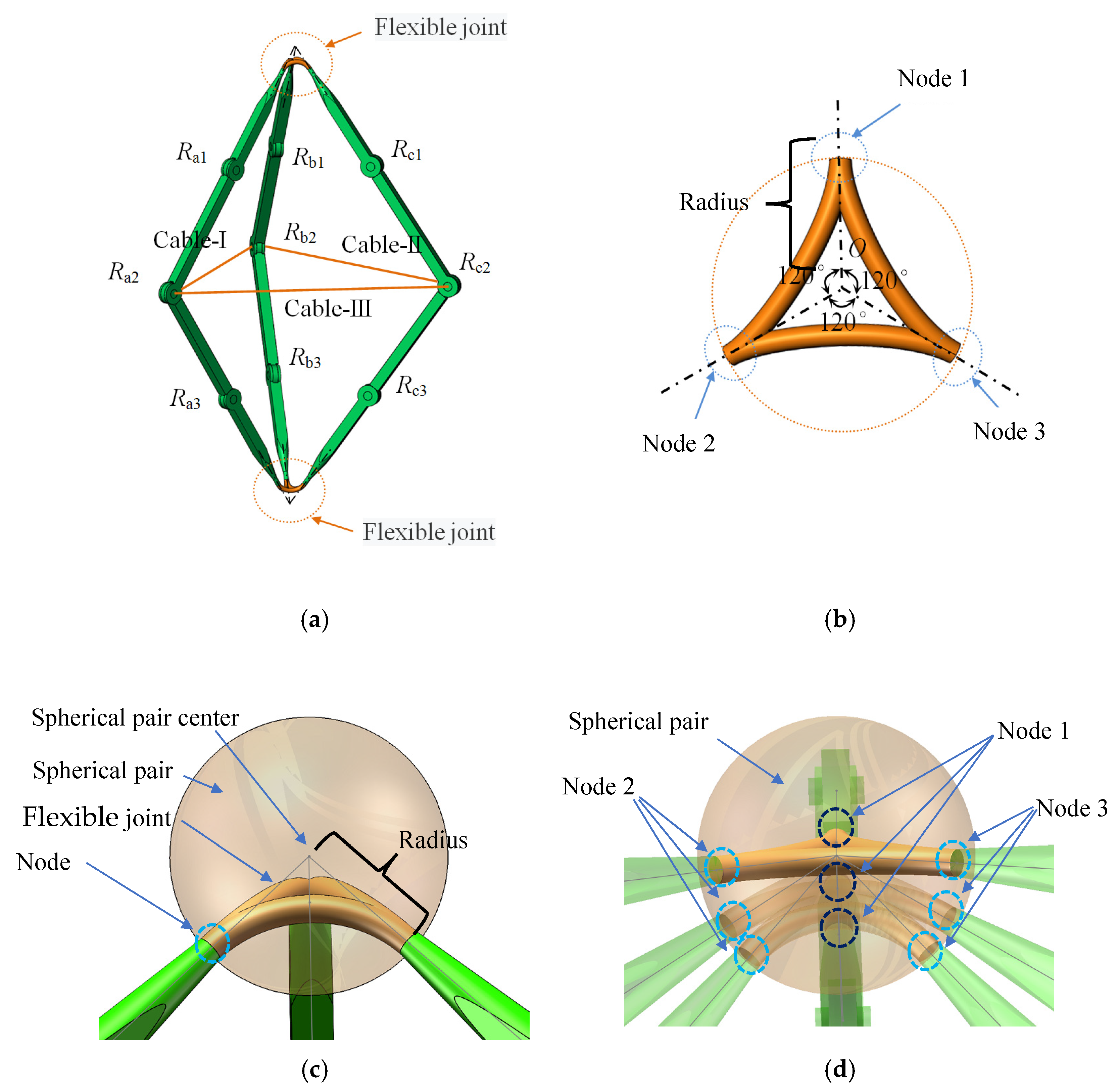
Figure 1. The rigid–flexible coupling rolling mechanism. (a) 3D model of the overall mechanism; (b) 3D model of the triangular flexible joint. (c) Flexible joint simplified model. (d) Schematic diagram of flexible joint deformation.
Machines 14 00227 g001
Figure 2. (a) Simplified mechanism diagram; (b) 3D model of the simplified mechanism.
Machines 14 00227 g002
Figure 3. The simplified model of the analysis diagram. (a) The branched chain A assembly diagram; (b) the branched chain A and the branched chain B overall assembly diagram; (c) simplified mechanism overall assembly diagram; (d) the angles between the planes where the branched chains are located are smaller than the π projection; (e) the angles between the planes where the branched chains are located are not all smaller than the π projection diagram.
Machines 14 00227 g003
Figure 4. Rolling process in star gait rolling mode. (a) Initial state of star gait rolling mode; (b) Direction selection of star gait rolling mode; (c) The rotating joint in the middle of the branch rotates; (d) Branched chain with double rotational pairs rotating; (e) Mechanism Toppling; (f) The rotating pair returns to its initial state; (g) The cable returns to its initial state.
Machines 14 00227 g004
Figure 5. Step size in star gait rolling mode.
Machines 14 00227 g005
Figure 6. The equivalent planar 8-bar mechanism: (a) general view; (b) projected view.
Machines 14 00227 g006
Figure 7. Initial state of rolling mode of the deformable triangular prism: (a) 3D model; (b) equivalent planar mechanism.
Machines 14 00227 g007
Figure 8. Rolling process of the deformable triangular prism. (a) Deformable triangular prism rolling initial state; (b) Branch b is inclined forward; (c) The branched chain a moves closer to the branched chain c; (d) Cable II further retraction; (e) the support area bc; (f) Supporting area bc expands; (g) The mechanism returns to initial state.
Machines 14 00227 g008aMachines 14 00227 g008b
Figure 9. (a) Equivalent plane position. (b) Schematic diagram of the equivalent planar mechanism in star gait rolling mode.
Machines 14 00227 g009
Figure 10. CoM workspace of the equivalent planar mechanism.
Machines 14 00227 g010
Figure 11. Two configurations for collision with the ground: (a) configuration −1 g; (b) configuration −2 g.
Machines 14 00227 g011
Figure 12. The input parameters when the step size is 320 3 mm with the impact minimum: (a) angle parameters; (b) flexible cable parameters.
Machines 14 00227 g012
Figure 13. Friction analysis schematic diagram; (a) Friction at branched chain C is greater than that at branched chain A; (b) Friction at branched chain A is greater than that at branched chain C.
Machines 14 00227 g013
Figure 14. Rolling motion: (a) equivalent planar mechanism; (b) CoM workspace projection.
Machines 14 00227 g014
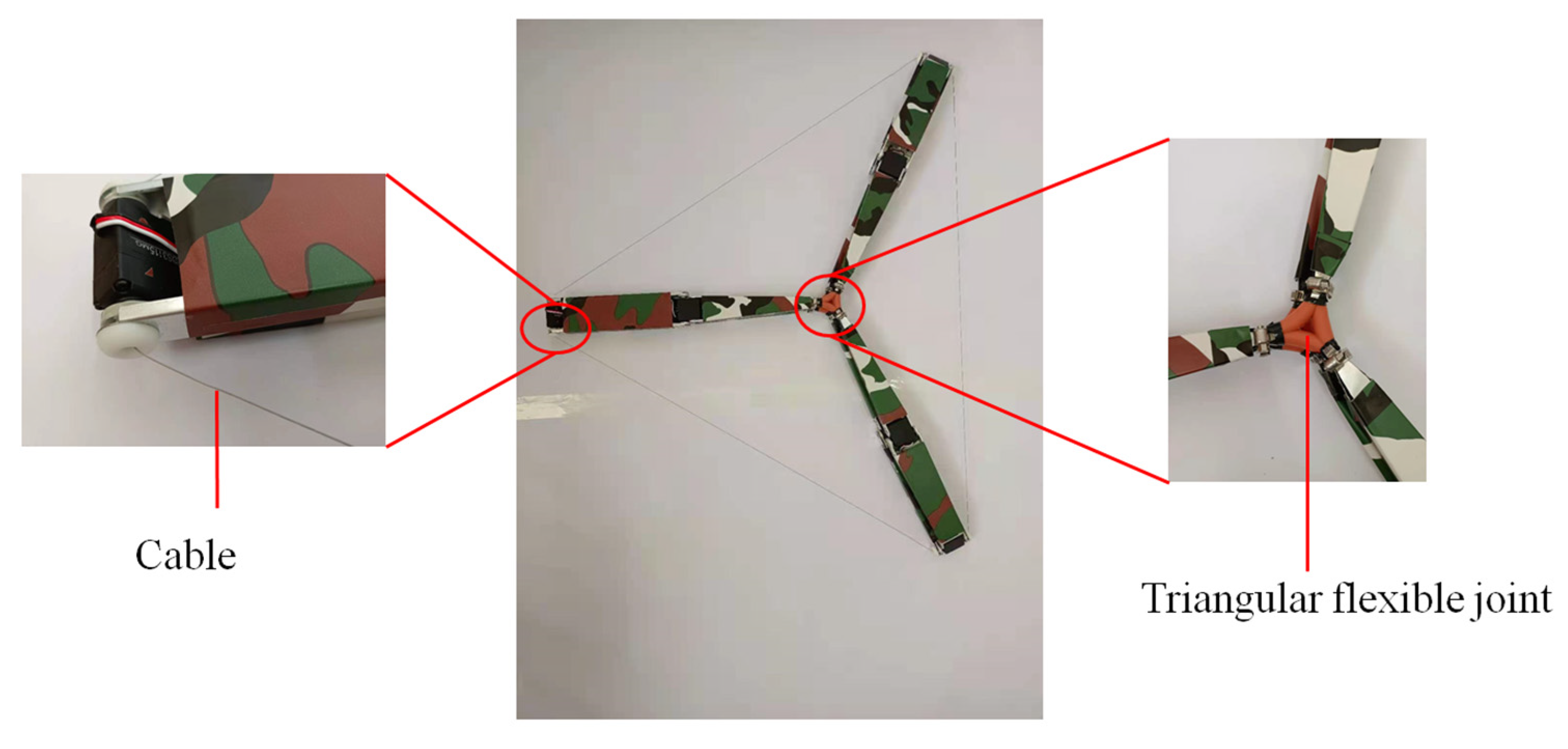
Figure 15. The prototype of the rigid–flexible coupling rolling mechanism.
Machines 14 00227 g015
Figure 16. The rolling process of the prototype in star gait rolling mode. (a) The motion state at the 0-s moment; (b) The motion state at the 2-s moment; (c) The motion state at the 3-s moment; (d) The motion state at the 4-s moment; (e) The motion state at the 5-s moment; (f) The motion state at the 6-s moment; (g) The motion state at the 7-s moment; (h) The motion state at the 9-s moment.
Machines 14 00227 g016
Figure 17. The rolling process of the prototype in the deformable triangular prism mode. (a) The motion state at the 0-s moment; (b) The motion state at the 3-s moment; (c) The motion state at the 44-s moment; (d) The motion state at the 7-s moment.
Machines 14 00227 g017
Table 1. Parameters of the prototype.
ParameterSpecification
Total weight3.0 kg
Total size580 mm × 510 mm × 490 mm (max)
MoterRDS3115: 4.8–6.8 V, 60 g, 0.16 s/60° (5 V), 15 kg·cm (5 V), 40 mm × 40 mm × 20 mm
Length of one linkl = 250 mm
Width of one linklW = 50 mm
Disclaimer/Publisher’s Note: The statements, opinions and data contained in all publications are solely those of the individual author(s) and contributor(s) and not of MDPI and/or the editor(s). MDPI and/or the editor(s) disclaim responsibility for any injury to people or property resulting from any ideas, methods, instructions or products referred to in the content.