Article

Linear Algebra-Based Multivariable Controller Design for Gas Turbine Machines with State-Derivative Feedback

by
Belkacem Bekhiti
1,
Kamel Hariche
2,
Abderrezak Guessoum
3 and
Abdel-Nasser Sharkawy
4,5,*
1
Institute of Aeronautics and Space Studies (IASS), University of Blida 1, BP 270, Blida 09000, Algeria
2
Institute of Electrical and Electronic Engineering (IGEE), University of Boumerdes, Boumerdes 35000, Algeria
3
Signal Processing and Image Laboratory (LATSI), Department of Electronics, Faculty of Technology, University of Blida, Blida 09000, Algeria
4
Mechanical Engineering Department, Faculty of Engineering, Qena University, Qena 83523, Egypt
5
Mechanical Engineering Department, College of Engineering, Fahad Bin Sultan University, Tabuk 47721, Saudi Arabia
*
Author to whom correspondence should be addressed.
Machines 2026, 14(2), 169; https://doi.org/10.3390/machines14020169
Submission received: 31 December 2025 / Revised: 24 January 2026 / Accepted: 27 January 2026 / Published: 2 February 2026
(This article belongs to the Section Automation and Control Systems)

Abstract

This paper presents a linear algebra-based control algorithm for multivariable gas turbine systems using matrix polynomial theory and the Kronecker product to assign block roots (i.e., block eigenvectors with prescribed latent structure). State and state-derivative feedback strategies are investigated and validated through simulations on an industrial gas turbine machine. The proposed method enables direct assignment of block roots governing closed-loop stability and transient response, while block eigenvectors shape the dynamic behavior of key turbine variables. Applicability of the approach requires block controllability and/or block observability, ensuring analytical transparency, design flexibility, and effectiveness for multivariable gas turbine control.

1. Introduction

The systematic design of multivariable controllers has its theoretical roots in linear algebraic formulations of pole placement. Early seminal work established the conditions under which arbitrary pole assignment is achievable in multi-input controllable linear systems through state feedback, laying the groundwork for modern MIMO control synthesis [1]. Subsequent developments extended this notion by demonstrating that state feedback offers structural freedoms beyond mere eigenvalue placement, enabling deeper manipulation of closed-loop dynamics and performance characteristics [2]. These insights motivated a broad class of eigenstructure-based design techniques, where both eigenvalues and eigenvectors are explicitly shaped to meet stability and dynamic response requirements. The algebraic characterization of eigenstructure (ES) assignment rapidly evolved toward parametric formulations, enabling systematic controller synthesis with explicit degrees of freedom. Early parametric solutions introduced tractable formulations for shaping closed-loop eigenstructures in multivariable systems [3], while complete ES-assignment frameworks formalized the simultaneous control of modal directions and dynamic modes [4]. These approaches were further generalized to aerospace and large-scale systems, where structural constraints necessitate refined algebraic tools [5]. Numerical algorithms addressing the computational challenges of eigenvalue assignment were subsequently proposed, emphasizing robustness and numerical efficiency [6]. Matrix polynomial theory emerged as a powerful framework for multivariable control, particularly for systems with complex interconnections and high dimensionality. The use of matrix polynomials enables controller synthesis through algebraic equations that directly encode system dynamics and desired closed-loop behavior [7]. Block pole placement strategies extended these ideas by introducing structured eigenvalue clustering, offering improved scalability for large MIMO systems [8]. Recent advances further integrate operator matrix polynomials into flight dynamics and aeroelastic control problems, highlighting their versatility in coupled physical phenomena [9].
While state feedback provides maximal flexibility, practical implementations often rely on output feedback due to sensing limitations. Reduced sensor-actuator configurations and output-feedback-based eigenvalue assignment techniques address this challenge by balancing performance and implementation complexity [10]. Robust ES-assignment methods explicitly incorporate uncertainties, ensuring stability and performance preservation under modeling errors [11]. Algebraic solution frameworks based on generalized Sylvester-type equations further unified eigenstructure synthesis for a wide class of linear systems [12]. Comprehensive theoretical treatments subsequently established rigorous conditions and classifications for ES-assignment problems [13]. Robust control formulations based on ES-assignment introduced multi-objective optimization into controller synthesis, enabling trade-offs between robustness, performance, and actuator constraints [14]. Parallel developments in intelligent and adaptive control demonstrated how algebraic controller structures can be embedded within learning-based frameworks [15]. These concepts were consolidated into authoritative monographs that formalized ES-assignment as a core paradigm in control theory [16]. Hybrid strategies combining genetic algorithms with gradient-based optimization further enhanced robustness and convergence properties in complex MIMO systems [17]. Efficient computation of matrix polynomial inverses and solvents is central to linear algebra-based control synthesis. Recursive schemes inspired by classical Leverrier–Faddeev algorithms have been proposed to address large-scale and high-order systems, with demonstrated effectiveness in structural dynamics applications [18]. Earlier foundational work on solvents and spectral factorization established the mathematical basis for such algorithms [19]. Non-iterative pole placement techniques subsequently refined these ideas, offering closed-form solutions with reduced computational burden [20].
Parametric static output feedback approaches provided additional flexibility for eigenvalue assignment without full state measurement [21]. These methods were extended to digital and adaptive control settings for large-scale MIMO systems, leveraging matrix Diophantine equations for systematic controller design [22]. Theoretical investigations into matrix polynomial solvents further deepened understanding of eigenvalue distributions in MIMO systems [23]. Recent studies revisited static output feedback gain design from an eigenspace characterization perspective, particularly for turbo-generator applications [24]. Block eigenvalue concepts introduced new solution paradigms for differential-matrix equations and descriptor systems [25]. State derivative feedback was shown to significantly enlarge the achievable eigenstructure set for descriptor systems, motivating renewed interest in derivative feedback strategies [26]. Matrix fraction descriptions further unified the treatment of large-scale descriptor systems within a polynomial framework [27], providing a natural foundation for state-derivative-based controller design.
Accurate gas turbine models are essential for high-performance controller synthesis. Data-driven identification techniques based on subspace methods have been successfully applied to capture dominant turbine dynamics from input–output measurements [28]. Advanced control-oriented modeling approaches have also enabled real-time emulation of gas turbine engines using electric machines, facilitating controller validation under realistic operating conditions [29]. Robust and nonlinear control strategies have been extensively investigated for gas turbine applications. Mixed-sensitivity H∞ control provided early robust design solutions for turbine systems [30], while sliding mode control emerged as a powerful alternative due to its robustness against uncertainties and disturbances [31]. Model-predictive control frameworks incorporating economic objectives further enhanced efficiency and operational flexibility [32]. Experimental validation of sliding mode load controllers confirmed their effectiveness in real-time turbine operation [33]. Earlier studies also demonstrated the stabilizing capability of sliding mode control for linear multivariable gas turbine models [34], while optimal LQG/LTR designs offered performance improvements in industrial settings [35].
Despite the extensive literature on ES-assignment, matrix polynomial methods, and gas turbine control, three critical gaps remain. First, most algebraic multivariable control frameworks focus on state or output feedback, with limited exploitation of state-derivative feedback despite its proven capability to expand ES-assignability. Second, existing gas turbine control strategies are predominantly numerical or optimization-driven, offering limited analytical transparency and structural insight. Third, there is a lack of unified linear algebra-based controller design frameworks that directly integrate multivariable pole assignment, matrix polynomial formulations, and gas turbine dynamics within a single coherent methodology. These gaps motivate the present work. The main contributions of this paper are summarized as follows:
  • Development of a linear algebra-based multivariable controller design framework incorporating vector spaces and state-derivative feedback.
  • Formulation of the controller synthesis problem using matrix polynomials.
  • Enhanced block-structure assignability compared to classical designs.
  • Application to a MIMO gas turbine model with transparent and flexible design.
  • Comparative study on a gas turbine showing the impact of the proposed method.
The remainder of this paper is organized as follows. Section 2 presents the mathematical preliminaries and problem formulation. Section 3 develops the proposed linear algebra-based controller synthesis with state-derivative feedback. Section 4 applies the methodology to a multivariable gas turbine model and discusses the results. The last section provides comparative analysis and performance evaluation. Finally, Section 5 concludes the paper and outlines directions for future research.

2. Mathematical Preliminaries

This paper is concerned with the control of the following high order dynamical linear system which is described by the following state and output equations [7]:
u t = k = 0 l A l k d k v t d t k ;       a n d         y t = k = 0 l 1 C l k d k v t d t k                          
Or more explicitly we can write
u t = A 0 d l v t d t l + + A l 1 d v t d t + A l v t   a n d y t = C 1 d l 1 v t d t l 1 + + C l 1 d v t d t + C l v t
where v t R m u t R m y t R p are the state vector, the control vector and the output vector, respectively. A i , R m × m with i = 0,1 , 2 , , l and C i R p × m i = 1 , 2 , , l are the system coefficient matrices where d e t ( A 0 ) 0 .
Now, by applying the Laplace transformation to Equations (1) and (2) we achieve the following dynamical equations:
                    u λ = A 0 λ l + A 1 λ l 1 + + A l v λ     a n d   y λ = C 1 λ l 1 + C 1 λ l 1 + + C l v λ               y t = N λ D λ 1 u λ            
where D λ = i = 0 l A i λ l i and N λ = i = 1 l C i λ l i . The matrices D λ   a n d   N λ are called matrix polynomials in complex variables λ with matrix coefficients which are defined on the field of real matrices R m × m .

2.1. Latent Structure and Block Roots (Solvents)

Definition 1 
([7]).  Let A k k = 0 l be a set of m × m complex matrices, then the matrix valued function A λ R m × m λ of the complex variable λ is called a matrix polynomial of degree l and order m where
A λ = A 0 λ l + A 1 λ l 1 + + A l 1 λ + A l = i = 0 l A i λ l i
Definition 2 
([8]).  The matrix polynomial A λ R m × m λ is called the following:
Monic if  A 0  is the identity matrix.
Comonic if  A l  is the identity matrix.
Regular if   det A λ 0 .
Nonsingular if  det A λ  is not identically zero.
Unimodular if  det A λ  is a nonzero constant.
Definition 3 
([9,24]).  The complex number   λ i C   is called a latent root of A λ if it is a solution of the scalar polynomial equation det A λ i = O m . The nontrivial vector p solution of A λ i p = O m is called a primary right latent vector associated with   λ i . Similarly, the nontrivial vector   q   , solution of q T A λ i = O m is called a primary left latent vector associated with   λ i . The term O m is the m × 1 or 1 × m zero matrix.
Remark 1. 
If the leading coefficient A 0 is singular, then A λ   has latent roots at infinity.
From the definition, we can see that the latent problem of a matrix polynomial is a generalization of the concept of the eigen-problem for square matrices. Indeed, we can consider the classical eigenvalues/vector problem as finding the latent root/vector of a linear matrix polynomial λ I A . We can also define the spectrum of a matrix polynomial A λ as being the set of all its latent roots (notation σ λ ). It is essentially the same definition as the one of the spectrum of a square matrix [22,23,24,25].
Definition 4 
([19]).  A right block root, also called the solvent of λ -matrix A λ is an m × m real matrix R in such a manner:
R l + A 1 R l 1 + A l 1 R + A l = O m or in other word A R R = i = 0 l A i R l i = O m
while a left solvent is an   m × m real matrix L in such a manner:
L l + L l 1 A 1 + L A l 1 + A l = O m or in other word A L L = i = 0 l L l i A i = O m
The following are important facts on solvents [8]:
  • Solvents of a matrix polynomial do not always exist.
  • Generalized right (left) eigenvectors of a right (left) solvent are the generalized latent vectors of the corresponding matrix polynomial.

2.2. Block Companion Forms

2.2.1. From Matrix Fraction Description to Block-State Space Realization

A linear time-invariant multivariable (MIMO) system expressed using a right matrix fraction description (RMFD) can be converted into a block state-space representation by applying a recursive procedure to the associated coupled differential equations [7].
Let now a dynamic system with the following RMFD:
y λ = H λ u λ = N R λ D R λ 1 u λ
D R λ   and N R λ   are m × m and p × m   matrix polynomials also called λ-matrices, the complex variable λ is often used instead of s, defined by the following:
D R λ = I m λ l + A 1 λ l 1 + + A l and   N R λ = C 1 λ l 1 + C 2 λ l 2 + + C l
where A i R m × m   constant matrices,   C i R p × m   are constant matrices, and   I m stands for the m × m identity matrix.
An alternative factorization of the matrix transfer function H λ   is called the left matrix fraction description (LMFD) and is defined by [8] the following:
H λ = N R λ D R λ 1 = D L λ 1 N L λ
Equation (6) represents a right and left matrix fraction description (MFD) of the matrix transfer function H λ R p × m λ . The terms N R λ R p × m λ , D R λ R m × m λ are the right numerator and denominator matrix polynomials, while the terms N L λ R p × m λ , and D L λ R p × p λ are the left numerator and denominator polynomials. For the equality to hold, the right and left MFDs must be equivalent, which requires D L λ N R λ = N L λ D R λ This is a polynomial matrix Diophantine equation.
The poles of H λ are the roots of D R λ (right MFD) or D L λ (left MFD).
The zeros are related to the determinants of N R λ , D R λ or N L λ , D L λ .
The general state space presentation of the given matrix fraction description, i.e., right or left, is obtained via the use of very well-known realization theory as follows [12,34]:
x ˙ t = A x t + B u t                         a n d                         y t = C x t + D u t
where A R n × n denotes the system matrix, B R n × m represents the input matrix, C R p × n is the output matrix, and D R m × p is the direct feedthrough matrix. The state, input, and output vectors are given by the following: x t   R n , u t R m , and y t R p   , respectively.

2.2.2. Transformation Between State-Space Forms

Consider a system represented by the standard state-space Equation (7), assumed to be controllable and/or observable. It can be converted into different companion forms—such as the controller or observer forms—through appropriate similarity transformations. [8]. In our study, three specific transformations are required: the block controller form, the block observer form, and the block diagonal form. To transform a system represented by A , B , C , D , the following conditions must be satisfied:
  • The number n / m = l   o r   n / p = l is an integer.
  • The matrix Ω = r o w A i B i = 0 l 1 = B , , A l 1 B   o r   Ω = c o l C A i i = 0 l 1 is of full rank.
Conversion to Block Controller Form
For a system defined by the general state-space model A , B , C , D that is block controllable, it can be converted into a block controller form [7,9]. If n / m = l is an integer and the block controllability matrix Ω c = B , A B , A l 1 B   is full rank, the state equation can be transformed into block controller form via the similarity transformation x c = T c x , where
x ˙ c t = A c x c t + B c u t                         a n d                         y t = C c x c t + D c u t
T c = T c l T c l A T c l A l 1 and T c l = O m , , O m , I m B , A B , A l 1 B 1
A c = O m I m O m O m O m O m O m O m I m A l A l 1 A 1 ,       B c = O m O m O m I m ,         C c = C l   , C l 1 , , C 1
with A c = T c A T c 1 , B c = T c B , C c = C T c 1 .
Conversion to Block Observable Form
If the considered system is block observable, then it can be transformed into a block observer form [7,9]. So if n / p = l is an integer number, and if the block observability matrix Ω o = C , A C , , A l 1 C   is full rank, then we can convert the state equation into block observer form using the following similarity transformation   x o = T o x
x ˙ o t = A o x o t + B o u t                         a n d                         y t = C o x o t + D o u t
T o = T o l , A T o l , , A l 1 T o l and T o l = C C A C A l 1 1 O p O p I p
A o = O p I p O p O p O p O p O p I p A l A 2 A 1 ,       B o = B l B 2 B 1 ,             C o = O p , , O p , I p
with A o = T o 1 A T o , B o = T o 1 B , C o = C T o .
Conversion to Block Diagonal Form
If the matrix polynomial A λ   possesses a complete set of solvents, then the companion matrices A c or A o can be block-diagonalized by right/left block Vandermonde matrices [25,27], defined as follows:
V R R 1 , , R l = I m I m I m R 1 R 2 R l R 1 l 1 R 2 l 1 R l l 1 , V L L 1 , , L l = I m L 1 L 1 l 1 I m L 2 L 2 l 1 I m L l L l l 1
V R R 1 , R 2 , , R l 1 A c V R R 1 , R 2 , , R l = blockdiag R 1 , R 2 , , R l
V L L 1 , L 2 , , L l   A o   V L L 1 , L 2 , , L l 1 = blockdiag L 1 , L 2 , , L l
These similarity transformations do a block decoupling of the spectrum of A λ   which is very useful in the analysis and design of large order control systems [15].

3. The Proposed Linear Algebra-Based Block Structure Assignment

3.1. Block Structure Assignment via State Feedback

This section introduces an alternative method for designing a linear state-feedback control law based on a desired left or right latent structure, using algebraic techniques and subspace theory. This approach serves as the MIMO counterpart to eigenstructure assignment, as discussed in prior studies [1,2,3,4,5,6].
Theorem 1 
([7]). Let   A c R n × n  denote a block companion controller form associated with the matrix polynomial A ( λ ) and let R i R m × m be a corresponding right block root (solvent). Then the following relation holds: A c X c i = X c i R i or equivalently
I m A c R i I n v e c X c i = 0   with   X c i = I m R i R i l 1
Here  X c i R n × m  represents the block eigenvector matrix (block vector),    denotes the Kronecker product, and  v e c ·  is the column-stacking operator.
Proof. 
This theorem can be readily verified by applying Definition 4 and performing direct algebraic manipulations. □
Theorem 2 
([8,9]).Every eigenvalue of a right or left solvent of A λ is also an eigenvalue of A c .
Proof. 
The block companion matrix A c   can be diagonalized using a block Vandermonde matrix through the similarity transformation: V R 1 A c V R = Λ = blckdiag R 1 , R 2 , , R l . Since d e t λ I n A c   =   d e t λ I n Λ   =   d e t blckdiag λ I m R 1 ,   , λ I m R l , it follows that d e t λ I n A c = d e t λ I m R 1 d e t λ I m R l . Hence, any eigenvalue of a right or left solvent R i   or L i of A λ is also an eigenvalue of A c . □
Remark 2. 
Assigning a matrix R  as a right solvent or a matrix   L   as a left solvent of   A λ , is equivalent to specifying the eigenvalues and eigenvectors of  R , or  L , as the latent roots and right or left latent vectors of A λ . In other words, assigning eigenvalues to a solvent of A λ directly corresponds to assigning these eigenvalues to the block companion matrix   A c [23,25].
Theorem 3 
([22,27]).  Suppose A λ has n linearly independent right latent vectors p 1 , , p n  (or left latent vectors q 1 , , q n ) associated with latent roots λ 1 , , λ n , then P Λ P 1 ,   Q 1 Λ Q   forms a right (or left) solvent of A λ , where  P = p 1 , , p n ,   Q = q 1 , , q n  and Λ = diag λ 1 , λ 2 , , λ n .
Consider the high-order dynamical system described by the state Equation (7). Applying the control law u t = K 1 x t + K 2 r t , the closed-loop equation becomes the following:
x ˙ t = A + B K 1 x t + K 2 r t
Bringing the system into a block controllable representation using: x c = T c x .
x ˙ c ( t ) = A c + B c K c 1 x c ( t ) + K c 2 r ( t )
To perform block pole assignment, we consider relocating the solvents of the plant. Let R i , X c i , denote the block eigen pairs, representing the complete set of desired solvents R i   with their corresponding block eigenvectors X i   w h e r e   i = 1,2 , , l . By the use of Theorem 1, we have the following:
A c + B c K c 1 X c i = X c i R i with i = 1 , 2 , l or equivalently
A c X c i X c i R i + B c K c 1 X c i = O n × m with i = 1 , 2 , l
Let the change in variable, W c i = K 1 c X c i A c X c i X c i R i + B c W c i = O n × m , then
I m A c R i I n v e c X c i + I m B c v e c W c i = O
  ( 22 ) I m A c R i I n I m B c v e c X c i v e c W c i = 0
Let us define the following matrices S R i = I m A c R i I n I m B c and X X c i , K c 1 = v e c X c i   v e c W c i . From standard linear algebra, it is straightforward to see that if S R i is singular, then Equation (23) admits a finite solution such that X X c i , K c 1 N S R i where N denotes the null space of S R i . Thus, X X c i , K c 1 from the kernel space of   S R i . Consequently, the block feedback matrices satisfy
W c R 1 , W c R 2 , , W c R l = K 1 c X c R 1 , X c R 2 , , X c R l
where W c i = W c R 1 and X c i = X c R 1 . A real feedback gain K c 1 exists if and only if the following conditions hold:
  • The assigned latent values are symmetric about the real axis.
  • The matrix V = X c R 1 , X c R 2 , , X c R l is nonsingular.
  • The complete set of desired solvents is constructed so that V R has full rank.
The feedback gain is then given by
K 1 c = W V 1
With W = W c R 1 , W c R 2 , , W c R l , V = X c R 1 , X c R 2 , , X c R l
K 1 = K 1 c T c
Some parameterization is necessary to obtain the feedback matrix that enforces the desired block structure. Consider the system A , B and define the following:
H 1 λ = N λ D 1 λ = λ I A 1 B λ · N λ = A · N λ + B · D λ
where the operation (●) stands for the dot-product and
  N λ = i = 0 l N i λ l i N i R n × m ,   D λ = i = 0 l D i λ l i D i R m × m with D 0 = I m × m , N 0 = O n × m  
The complete set of desired solvents satisfies Equation (27), giving the following:
N R i R i = A · N R i + B · D R i i = 1 , , l
With   N R i = N l , , N 0 I m R i R i l and   D R i = D l , , D 0 I m R i R i l
The closed-loop system with ( u t = K 1 x t + r t   where K 2 is designed out) can be expressed parametrically as follows:
H 2 λ = N λ D n e w 1 λ = λ I A B K 1 B λ · N λ = A · N λ + B · D n e w λ + B · K · N λ
Evaluating Equation (29) at a right solvent R i yields
N R i R i = A · N R i + B · D n e w R i + B · K · N R i i = 1 , , l
Remark 3. 
The assigned block eigenvalues are solvents of D n e w λ , hence  D n e w R i = O m × m .
In a more compact form, Equation (30) can be expressed as follows:
N l , , N 1 V R Λ R A + B K N l , , N 1 V R = O n × n           Λ R = N l , , N 1 V R 1 A + B K N l , , N 1 V R = V R 1 A c n e w V R
where
A c n e w = N l , , N 1 1 A + B K N l , , N 1
V R = B l o c k - V a n d e r m o n d M a t r i x
Λ R = B l o c k - d i a g o n a l M a t r i x
T c = N l , , N 1 1
Remark 4. 
If X c i  is a block eigenvector of the block companion matrix   A c ,   then the corresponding eigenvector in the original coordinates is  X i = T c 1 X c i   w h e r e   X i , X c i R n × m   i = 1 , , l .
X i = T c 1 X c i = T c 1 c o l R i k k = 0 l 1 = N l , , N 1 c o l R i k k = 0 l 1 = k = 0 l N l k R i k = N R i
E q u a t i o n s   28 a n d 30 K · N R i = D R i   K = D R 1 , D R 2 , , D R l N R 1 , N R 2 , , N R l 1
K c = D R 1 , D R 2 , , D R l N R 1 , N R 2 , , N R l 1 N l , , N 1
Now we should develop an algorithmic procedure to reconstruct the matrix coefficient   N i   and   D i . Expanding Equation (27), gives the following:
A N l + B D l = O                                                                                       A N i + B D i = N i + 1 i = 1 , , l 1 N 0 = O n × m                                                                                                           D 0 = I m × m                                                                                                              
From Equation (33) solving from the above with back substitutions, we obtain:
D l D 1 = B ,   A B ,     , A l 1 B 1 A l B = Ω c 1 A l B
N l , , N 1 = B , , A l 1 B D l 1 D 1 D 0 D 1 D 0
The complete procedure for computing the block pole-placement gain using right block root assignment is summarized in Algorithm 1.
Algorithm 1 Block-Controllability-Based Pole Placement Using Right Block Roots
Step 1:Verify that the system is block controllable and determine the controllability index l . Ensure that the matrix Ω c = B , A B , , A l 1 B is full rank and that   n = m l . If n is not integer multiple of m apply the method proposed by Bekhiti et al. [7].
Step 2:Transform the system into block controller form with l 2 sub-blocks using T c ·
Step 3:Construct the desired right block roots based on the specified latent structure, ensuring that   V R R 1 , R 2 , , R l is nonsingular.
Step 4:Compute the matrix coefficients   N i and D i ·
Step 5:Compute K c 1 = W V 1 N l , N l 1 , , N 1 with W = D R 1 , D R 2 , , D R l , V = N R 1 , N R 2 , , N R l and recover the original gain via, K 1 = K c 1 T c ·
Remark 5. 
Also, we can assign left block poles using only the transposition and duality.
Example 1. Consider the 2-by-2-output system described by the following state space model:
A = 2.25 2.25 0.25 1.25 5.00 4.25 0.50 1.75 1.25 1.25 1.25 0.25 0.50 0.25 1.00 0.75 , B = 4 6 2 4 2 2 0 2 , C = 4.5 9 3.5 1.5 3.5 5 4.5 3.0 , D = O 2 × 2
Block controllability is ensured because the matrix B , A B   is full rank with rank equal to 4, which gives a controllability index of l = n / m = 2 . In the same manner, the system is block observable, as r a n k C ,   C A = 4 , leading to an observability index of l = n / p = 2 . Hence, the entire state vector is observable and can be accurately estimated.
T c l = O 2 , I 2 B , A B 1 , T c = T c l T c l A = 0.0000 0.6667 1.5000 0.8333 2.0000 0.6667 4.0000 2.8333 2.0000 2.0000 0.5000 1.1667 2.0000 1.3333 3.0000 2.5000
The associated λ-matrix can therefore be expressed as follows:
A λ = 1 0 0 1 λ 2 + 4.5000 4.0000 2.3333 0.5000 λ + 2.1667 2.5000 3.5000 3.0000
The goal is to place the system block poles according to a desired latent structure.
2 , 2.5 , 7 , 14 , 0.9705 0.2322 0.2409 0.9727 0.9705 0.1787 0.3102 0.9839
Accordingly, the desired block roots R i  and their associated block eigenvectors X i  can be constructed according to [7] as follows:
R 1 = 6.5590 1.3517 2.4279 14.441 , X 1 = 40.3015 78.2392 25.1617 55.5606 16.1399 24.1786 8.5218 31.3819 ;   R 2 = 1.9685 0.1269 0.1319 2.5315 , X 2 = 6.5825 12.6966 5.7427 10.8798 1.8398   3.3168   3.4028 7.5630  
Applying the proposed method, the matrices D i   a n d   N i  can be derived from the system as follows:
            N 2 = 0.5000 3.0000 2.3333 0.5000 1.8333 2.0000 3.6667 2.5000 ,     N 1 = 4 6 2 4 2 2 0 2 , N 0 = O 4 × 2 D 2 = 2.1667 2.5000 3.500 3.0000 , D 1 = 4.5000 4.0000 2.3333 0.5000 , D 0 = I 2 × 2
Combine the obtained results to parametrically compute the feedback gain matrix that assigns the following block eigen pairs  X 1 , R 1 , ( X 2 , R 2 )  to the given system:
N R 1 = 40.3015 78.2392 25.1617 55.5606 16.1399 24.1786 8.5218 31.3819 ,   N R 2 = 6.5825 12.6966 5.7427 10.8798 1.8398 3.3168 3.4028 7.5630   D R 1 = 2.6803 77.5664 63.9972 206.3270 ,   D R 2 = 2.3056 7.6260 0.4336 4.9536  
K 1 = D R 1 D R 2 N R 1 N R 2 1 = 14.2169 5.8068 24.6660 3.6878 34.7681 17.1882 50.2814 10.9354
To achieve static tracking of a desired trajectory, the static gain matrix is designed as follows:
K 2 = H 0 + = C n e w λ I A n e w 1 B n e w λ = 0 + = C A + B K 1 B +
K 2 = 1.6098 8.9335 5.2640 21.4814
where +   denote the pseudo-inverse.

3.2. Block Structure Assignment via State Derivative Feedback

This section addresses a feedback strategy that relies solely on state derivatives, rather than full-state measurements, and is therefore referred to as state-derivative feedback [26]. Naturally, this leads to the problem of block-structure assignment using such feedback. Consider a linear, time-invariant system that is completely controllable:
x ˙ t = A x t + B u t ;   x t 0 = x 0
where x t R n   is the state vector, u t R m   is the control input m < n , and A R n × n , B R n × m are the system and input matrices, respectively. It is assumed that the system is completely block controllable with a controllability index ( l = n / m ) and that B has a full column rank m.
The goal is to stabilize the system via a linear feedback law that enforces a desired dynamic behavior. The block-structure assignment problem consists of finding a state-derivative feedback control law:
u t = K 1 x ˙ t + K 2 r t
which assigns the prescribed closed-loop latent values and associated latent vectors (or the target block roots), ensuring system stability and desired performance [7]. The resulting closed-loop dynamics are as follows:
x ˙ t = I n B K 1 1 A x ( t ) + I n B K 1 1 B K 2 r ( t )
Transforming the system into block controller coordinates via x c t = T c x t gives the following closed-loop state equation:
x ˙ c ( t ) = I n B c K c 1 1 A c x c ( t ) + I n B c K c 1 1 B c K c 2 r ( t )
where I n R n × n is the identity matrix. It is assumed that I n + B c K c 1 is nonsingular, so the closed-loop system is well-defined. The corresponding characteristic polynomial satisfies the following:
d e t λ I n I n B c K c 1 1 A c = 0
Denote the right block-eigenvector matrix of A n e w = I n B c K c 1 1 A c   by   X c i   , and we then have by definition: I n B c K c 1 1 A c X c i = X c i R i with i = 1,2 , , l
A c X c i = I n B c K c 1 X c i R i A c X c i X c i R i = B c K c 1 X c i R i with i = 1,2 , , l
Letting W c i = K 1 c X c i we will receive the following matrix equation:
A c X c i X c i R i = B c W c i R i with i = 1,2 , , l
Using the Kronecker product, this can be compactly written as follows:
I m A c R i I n R i B c v e c X c i v e c W c i = O
Define the following structured matrices S R i = I m A c R i I n R i B c and X X c i , K c 1 = v e c X c i   v e c W c i . As shown previously, if S R i is singular, a finite solution to (43) exists such that X X c i , K c 1 N S R i where N denotes the null space of the matrix S R i . Hence, X X c i , K c 1 can be constructed from the kernel space of the matrix S R i .
Remark 6. 
When the desired block poles are repeated, the corresponding block eigenvectors can be generated iteratively as: A X k = X k R i + X k 1   or v e c X k = I m   A R i I n 1 v e c X k 1 .
Similarly to the previous case, we need to parametrically determine the feedback gain matrix that assigns the full block structure using state-derivative feedback. The resulting closed-loop transfer function of the system A , B is given by
H λ = λ I n I n B K 1 1 A 1 I n B K 1 1 B = N λ D n e w 1 λ = λ I n B K 1 A 1 B = N λ D n e w 1 λ
This leads to
B · D n e w λ = λ I n B K 1 A · N λ
After simplification of Equation (44) we have the following:
λ · N λ = A · N λ + λ · B · K 1 · N λ + B · D n e w λ
The complete set of desired solvents satisfies Equation (45), giving
N R i R i B · K 1 · N R i R i = A · N R i + B · D n e w R i i = 1 , , l
Combining Equations (28) and (46) results in the matrix relation:
K 1 N R i R i = D R i i = 1 , , l
In a more compact form, this can be expressed as
K c 1 = W V 1 N l , N l 1 , , N 1 where K 1 = K c 1 T c
With W = D R 1 , D R 2 , , D R l , V = N R 1 , N R 2 , , N R l
Example 2. 
Consider the 2-by-2 system represented by the following state space model
A = 10.1053 13.5732 7.0930 22.2085 5.0500 6.5831 2.0206 8.4311 8.4457 10.0912 5.1693 18.1104 5.3245 6.8585 4.2611 12.6915 , B = 7.1233 10.8439 3.7903 5.4963 4.4474 8.3113 2.5707 4.9250 C = 0.2226 0.0658 0.7645 0.5436 0.3164 1.1572 0.3873 0.9099 ,                   D = O 2 × 2                                                    
The system is block controllable since the matrix B , A B , A 2 B , A 3 B   has full rank, giving a controllability index l = n / m = 2   so that, Ω c = B , A B . The desired closed-loop latent structures (latent roots and corresponding latent vectors) are chosen as follows,
  10 , 5 , 1.5 , 3 , 0.8697 0.7632 0.4935 0.6461 0.8828 0.1950 0.4698 0.9808
This defines the next block roots and their corresponding block eigenvectors to be assigned:
R 1 = 20.1658 17.9154 8.6055 5.1658 , X 1 = 40.6166 60.0765 23.5804 32.7722 7.1815 21.7943 3.6278 12.5329 ;   R 2 = 1.3225 0.3335 0.8927 3.1775 , X 2 = 9.3877 20.5580 4.3636 9.4607 2.3202 9.9778 1.9660 6.7112
In this example, the goal is to design a state-derivative feedback control law of the form: u t = K 1 x ˙ t + K 2 r t   , so that the desired latent structure (block roots) is assigned to achieve the specified performance. Applying the proposed state-derivative feedback procedure, the matrices D i   a n d   N i can be derived from the system matrices:
N 2 = 9.7132 11.5229 5.5556 6.7398 10.9810 14.9481 5.8303 8.0806 , N 1 = 7.1233 10.8439 3.7903 5.4963 4.4474 8.3113 2.5707 4.9250 ,         N 0 = O 4 × 2 D 2 = 0.7345 2.5844 3.1428 6.1675 ,   D 1 = 1.3344 4.3346 2.2342 5.3344 , D 0 = I 2 × 2
The feedback gain matrix can then be constructed from the obtained results:
N R 1 R 1 = 300.0791 417.3205 193.4962 253.1573 42.7302 16.0744 34.6945 0.2510 , N R 2 R 2 = 30.7673 62.1922 14.2164 28.6060 11.9757 30.9307 8.5911 20.6693 D R 1 = 241.3619 267.6612 125.0898 133.7889 ,   D R 2 = 6.3509 9.2428 0.5569 0.2386
K c 1 = D R 1 D R 2 N R 1 R 1 N R 2 R 2 1 N 2 N 1 = 0.6496 2.1549 1.2084 0.4517 0.4303 1.7686 0.2692 0.4933
K 1 = K c 1 O 2 I 2 B A B 1   O 2 I 2 B A B 1 A = 0.4272 0.3291 0.4058 1.9012 0.8686 1.0059 1.6732 3.7137
The static pre-compensation gain is determined as follows:
K 2 = H 0 + = C A + B K 1 B + = 2.9525 9.2726 3.7843 11.3856
The latent-structure (block-root) assignment method has been demonstrated as a tool for designing both state and state-derivative feedback controllers, producing a closed-loop system with prescribed characteristics. This approach ensures stability when the necessary and sufficient conditions are satisfied. Compared to conventional state feedback, the state-derivative feedback controller can, in certain cases, achieve equivalent performance with smaller gain values. From a practical standpoint, minimizing feedback gains is desirable, as lower gains result in smaller control signals and reduced energy consumption [7,27].

4. Application to the Gas Turbine Machine

4.1. The Gas Turbine Machine Control via the Proposed Method

This section studies the GE MS5001P gas turbine at M’SILA power plant (Algeria), selected for its available real-time data. The plant has 22 single-shaft turbines driving the main generators. Each turbine includes an axial compressor, a combustion chamber, and a multi-stage turbine. Rare start-up/shutdown transients are excluded [29,30,31,32]. Key characteristics of this gas turbine machine are in Table 1.
The single-shaft industrial gas turbine GE MS5001P is considered to operate in the vicinity of a nominal steady-state condition under ISO ambient conditions. The dynamic model is derived by linearizing the nonlinear thermodynamic equations about a selected equilibrium (trim) point [34].
Assumptions:
  • Lumped-parameter model;
  • Ideal gas behavior;
  • Small perturbations around equilibrium;
  • No variable geometry;
  • Neglecting shaft torsional flexibility.
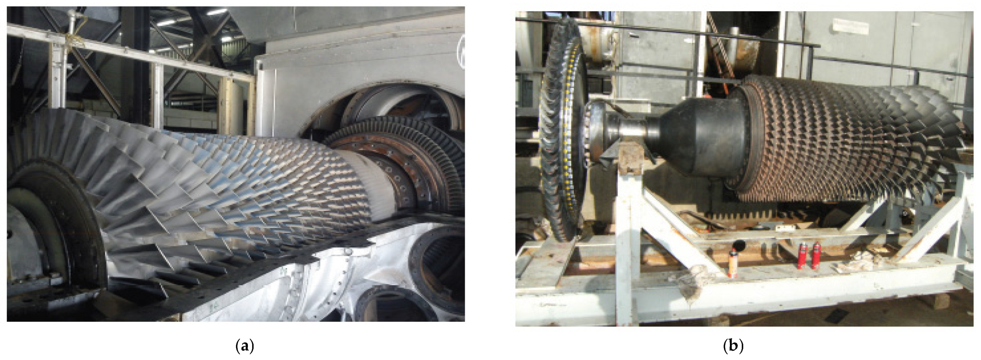
Numerous parameters influence gas turbine dynamics (Appendix A), with their impact varying according to their role within the main sections of the turbine, namely the compressor, the combustion chamber, and the turbine. In this study, the modeling effort is deliberately restricted to the two principal output variables of the GEMS5001P gas turbine under normal operating conditions: the rotor speed and the exhaust gas temperature. These outputs are directly affected by, and dynamically coupled with, three main variables: the gas control valve (GCV), the axial compressor discharge temperature (TCD), and the axial compressor discharge pressure (PCD) [28]. Figure 1. illustrates the axial compressor of the GE 5001P gas turbine and the turbine section of the same system.
The overall dynamics of the gas turbine can be described by a nonlinear multivariable state–space model that captures the coupled mechanical, thermodynamic, and fluid-flow phenomena of the compressor–combustor–turbine assembly. The nonlinear model is expressed as x ˙ = f x t , u t ;   y = h x t where x R 6 , u R 2 , and y R 2 . The state vector is defined as x t = ω r , T C D , P C D , T t , T E , τ s with ω r is the rotor speed, T C D and P C D are the compressor discharge temperature and pressure, T t is the turbine inlet temperature, T E is the exhaust gas temperature, and τ s is the shaft torque. These states describe the dominant nonlinear interactions between the rotating shaft dynamics and the thermal processes occurring in the compressor, combustor, and turbine. The input vector is given by u t = C G V , T C D r e f where C G V denotes the gas control valve position governing the fuel mass flow rate into the combustor, and T C D r e f is the input compressor discharge temperature, which indirectly affects combustion efficiency and downstream thermal dynamics [30,31,32,33]. The complex nonlinear model can be written as
d d t ω r T C D P C D T t T E τ s = η t m ˙ f c p T t T E η c m ˙ a c p R T C D T C D r e f J ω r τ s / J ω r T C D r e f T C D + k 1 ω r ω r 0 + k 2 P C D P C D 0 + k 3 m ˙ f / τ C D P C D s s ω r , m ˙ f P C D / τ P α f m ˙ f + β a T C D T C D r e f T t / τ t T t T E + γ ω r ω r 0 / τ E k t τ t τ c τ s / τ τ
where J is the shaft inertia. η t , η c are the turbine and compressor efficiency factors. m ˙ f is the fuel mass flow rate (controlled via GCV m ˙ f = k G C V u 1 ). m ˙ a is the air mass flow rate through the compressor. c p , R are the specific heats. k 1 , k 2 , k 3 are gains capturing rotor-compressor coupling, and τ C D is the thermal time constant. P C D s s ω r , m ˙ f is the steady-state compressor pressure as a function of rotor speed, τ P is the pressure time constant. α f ,   β a representing the effect of fuel flow and compressed air on turbine temperature. γ captures the dynamic coupling between rotor speed and exhaust gas temperature, τ E is exhaust thermal constant. k t is a mechanical gain and τ τ is the shaft torque time constant. The measured outputs are selected as y t = ω r , T E since rotor speed and exhaust gas temperature are the most relevant performance indicators during normal operating conditions.
This is now a completely explicit nonlinear model, including all six states, two inputs, and the outputs. It is suitable for simulation, control design, and linearization. The linear model is obtained by linearization around a steady operating point  x 0 , u 0 . The states’ deviations considered are as follows: the rotor speed x 1 = ω r , the compressor discharge temperature x 2 = T C D , the compressor discharge pressure x 3 = P C D , the turbine inlet temperature x 4 = T t , the exhaust gas temperature x 5 = T E , and the shaft torque x 6 = τ s . These states capture the dominant interactions among the compressor, combustor, and turbine, including both thermal and mechanical dynamics. The system is influenced by two independent inputs: the gas control valve u 1 = G C V , which modulates the fuel flow into the combustor, and the compressor discharge temperature reference u 2 = T C D r e f , which affects the air–fuel mixture and consequently the downstream thermal states. The two measured outputs are the rotor speed and the exhaust gas temperature, denoted as y 1 = ω r and y 2 = T e , which are the primary indicators of turbine performance in normal operating conditions [28,30].
Finally, the linear model is obtained by linearizing the nonlinear dynamics around a nominal steady-state operating point x 0 , u 0 , corresponding to normal turbine operation, leading to the deviation model x ˙ = A · x t + B · u t ;   y t = C · x t . The operating point is computed by solving the trimming conditions f x , u = 0 using optimization-based methods. The state-space matrices A , B , and C can, in principle, be obtained by evaluating the Jacobians of the nonlinear system x ˙ = f x t , u t ;   y = h x t at the nominal operating point x 0 , u 0 . However, since many of the physical constants and parameters are not known a priori, an identification-based approach is employed to derive an approximate continuous linear model that accurately captures the system dynamics around the operating point [34].

4.2. Recursive Methods for Continuous Time System Identification

The multivariable continuous time recursive least square (MCTRLS) is an algorithm stated to minimize the criterion
J = 0 t φ τ θ τ y τ 2 d τ     θ 0 t e 2 τ d τ = 2 0 t φ τ φ τ θ τ y τ d τ = 0
So that the least square estimate is
θ t = 0 t φ τ φ τ d τ 1 0 t φ τ y τ d τ
For adaptive control applications, we are interested in recursive formulation where the parameters are updates continuously on the basis of input output data. Such update may be obtained by defining
P t = 0 t φ τ φ τ d τ 1           d d t P 1 t = φ t φ t
We use the fact that
d I d t = d d t P t P 1 t = d P d t · P 1 t + P t · d P 1 d t = 0         d P d t = P t d P 1 d t P t = P t φ t φ t P t
On the other hand
θ t = P t 0 t φ τ y τ d τ       d θ d t = P t φ t y t P t φ t φ t θ t = P t φ t e t
Finally, we can write (with some forgetting Factor) this steps in Algorithm 2.
Algorithm 2 Multivariable Continuous Time Recursive Least Square
Step 1:Input u t , y t and form the data matrix ϕ t If we define the matrix R t = P 1 t then
Step 2: d θ d t = P t ϕ t e t d θ d t = R 1 t ϕ t e t
Step 3: e t = y t ϕ t θ t e t = y t ϕ t θ t
Step 4: d P d t = α P t P t ϕ t ϕ t P t d R d t = ϕ t ϕ t α R t
Linear continuous-time systems can be described in two main ways: the state-space (internal) representation, which captures the system’s dynamics via state variables, and the input-output representation, expressed either as a time-domain differential equation or as an n t h order transfer function in the s-domain. Previously, we reviewed identification methods based on numerical integration, which require measurements of all states and inputs. In contrast, the method presented here relies only on the input sequences and a single output sequence to estimate the continuous-time system parameters.
The trapezoidal rule approximates the integrand y t by a linear function over each interval k 1 T t k T . Within this interval, the linear approximation—known as a trapezoidal pulse function—can be expressed as follows:
f y = k T t T y k 1 t k 1 T T y k ;                       f o r     k 1 T t k T
Here, y k denotes y k T . The identification method requires successive integrals of y t to estimate the continuous-time system parameters. Accordingly, a set of approximate formulas is used to compute these integrals. Over the interval k 1 T t k T , the area under the linear approximation of y t equals the standard trapezoidal integral. The recursive formula for the first and second integral of y t then can be expressed as follows:
I 1 , k = I 1 , k 1 + T 2 y k 1 + y k ;         a n d         I 2 , k = I 2 , k 1 + T · I 1 , k 1 + T 2 3 ! 2 y k 1 + y k
In general, we can express the n t h integral of y t by the following equation
  I 1 , k = i = 1 n T n i i 1 ! I n i + 1 , k 1 + T n n + 1 ! n y k 1 + y k  
Now, the identification problem can be easily solved by simple applying this equation to the differential equation of continuous-time systems. Consider the MIMO continuous-time system described by I λ n + i = 1 n D i λ n i y λ   = i = 0 m N i λ m i u λ or by
D λ y λ = N λ u λ d n y t d t n + i = 1 n D i d n i d t n i y t = i = 0 m N i d m i d t m i u t
The identification problem now is to estimate the parameters D i and N i . Integrating both sides of the above equation n times with respect to t over the subinterval k 1 T t k T , we obtain
Δ y k + i = 1 n D i Δ I i , k y = i = 1 m N i Δ I i , k u             w i t h             Δ y k = y k y k 1
where the differences are Δ y k = y k y k 1 , Δ I i , k y = I i , k y I i , k 1 y and Δ I i , k u =   I i , k u I i , k 1 u . The quantities I i , k y and I i , k u are the i t h integrals of y and u at the k t h sampling instant, respectively.
A multivariable continuous-time identification is performed via a trapezoidal integration–based recursive least squares (RLS) scheme as shown in Algorithm 3.
Algorithm 3 Multivariable Continuous Time Trapezoidal Integral RLS (For a 2nd order MDFD model)
1Given:
2
  • Sampling period  T s = t , final time  t F
3
  • Input  u k R m , output  y k R p
4
  • Number of samples  N = r o u n d t F / t ,
5
  • The overall time grid  t = 0 : t : t F
6%-----Initial Values-----%
7 θ 1 = O ,   w i t h   θ R 8 × 2 ; % with θ = [D1;D2;N1;N2]
8 P 1 = α × I 8 R 8 ; α = 10 15 ; % Covariance matrix
9 S 1 y = 0     0 ; S 1 u = 0     0 ; I 2 y = 0     0 ; I 2 u = 50     0 ; % Initialize integral states
10
11%-----Data Acquisition-----%
12For k = 1:N, y k = D u k ; End  % where D represents the real system dynamics. 
13For k = 2:N-1
14%-------Integrations-------%
15                 I k + 1 y = y k + 1 + y k · T s / 2 ; I k + 1 u = u k + 1 + u k · T s / 2 ; % Local trapezoidal integrals
16                 S k y = S k 1 y + I k y ; S k u = S k 1 u + I k u ; % Cumulative 1st integral
17                 I k + 1 y = S k y · T s + 2 · y k + y k + 1 · T s 2 / 6 ; % Local 2nd order integrals
18                 I k + 1 u = S k u · T s + 2 · u k + u k + 1 · T s 2 / 6 ;
19%-------RLS Algorithm-------%
20                 y k = y k + 1 y k ; % Output increment
21                 ϕ k = I k + 1 y ; I k + 1 y ;   I k + 1 u ;   I k + 1 u ; % Regressor vector
22                 K k = P k 1 · ϕ k / 1 + ϕ k · P k 1 · ϕ k ; % RLS gain
23                 θ k = θ k 1 + K k · y k ϕ k · θ k 1   ; % Parameter update
24                 P k = P k 1 K k · ϕ k · P k 1 ; % Covariance update
25End
As discussed previously, it is often preferable to identify the parameters of a continuous-time system directly from discrete input-output measurements. The core concept is to integrate the system’s differential equations over each sampling interval, yielding relationships between the sampled input-output data and the unknown model parameters. For instance, consider a state-space representation where the state x t is assumed measurable and e t is a white noise process. x ˙ t = A x t + B u t + e t where x R n , e R n , and u R m . The terms A , B , are parameter matrices. The objective is to identify the system matrices from sampled input–state data u t and x t collected at t = k T , for k = 0 , , N . The sampling period T is assumed sufficiently small to preserve the system dynamics. In practice, the identification is complicated by measurement noise.
If we integrate the differential equation in x ˙ t = A x t + B u t + e t between the limits t k 1 = k 1 T and t k   =   k T , we obtain d t   = t k t k 1 =   T and
x k = x t k x t k 1 = A t k 1 t k x t d t + B t k 1 t k u t d t + t k 1 t k e t d t = A       B I x t k I u t k + I e t k
Therefore,
x k = θ φ k t k + I e t k                     x k = I x t k       I u t k A B + I e t k = φ k t k θ + I e t k
With I x t k = t k 1 t k x t d t ;   I u t k = t k 1 t k u t d t ;   a n d   I e t k = t k 1 t k e t d t
Exact evaluation of the integrals is infeasible since only noisy samples of x t k , and u t k are available. Therefore, the integrals are approximated using sampled data under an assumed model structure. Numerical integration–based identification methods are adopted, assuming a minimal (controllable and observable) system realization. If we choose a trapezoid to approximate the area of a typical panel, then we have the Trapezoidal rule, that is
I x t k = t k 1 t k x t d t x k + 1 + x k 2 T ;           a n d           I u t k = t k 1 t k u t d t u k + 1 + u k 2 T
Means that
x t k + 1 x t k = A x k + 1 + x k 2 + B u k + 1 + u k 2 T
  x t k + 1 = I A T 2 1 I + A T 2 x t k + T I A T 2 1 B u k + 1 + u k 2 = A d x t k + B d u 0 t k
W h e r e       A d = I A T 2 1 I + A T 2 ;   B d = T I A T 2 1 B ;   u 0 t k = u k + 1 + u k 2
By using this identification method we see that the discrete-time system obtained is identical to the one calculated by the bilinear z transformation. Clearly, if we have all the state measurements and the input samples, the parameters A and B can be easily estimated by applying the least squares approach
x k = φ k t k θ + I e t k         x 1 x 2 x n = t 0 t 1 x t d t                     t 0 t 1 u t d t                                                                               t n 1 t n x t d t                     t n 1 t n u t d t A     B + t 0 t 1 e t d t   t n 1 t n e t d t
Or in compact form we write
x k = φ k t k θ + I e t k         x 1 x n = I x t 1                     I u t 1                                           I x t n                     I u t n A   B + I e t 1 I e t n         X = ϕ θ + ε
By using the ordinary least square we obtain θ = ϕ ϕ 1 ϕ X + ϕ ϕ 1 ϕ ε whose optimal values is given by
θ = ϕ ϕ 1 ϕ X
where the matrix ϕ can be approximated by
ϕ = I x t 1   I u t 1   I x t n   I u t n 1 2 x 1 + x 0   u 1 + u 0     x n + x n 1   u n + u n 1 1 2 ϕ x + ϕ u
Now let us implement this identification method using Algorithm 4.
Algorithm 4 Multivariable Continuous Time Identification (For a Gas Turbine Model)
1Given:
2
  • t = 0.0001 ,
% Sampling period
3
  • t 1 = 0 , t F = 5.0
% Initial and final time
4
  • u k R m , x k R n ,
% Input and state vectors
5
  • θ R 8 × 6
% Parameter matrix   θ = A ; B
6
  • N = r o u n d t F / t ,
% Number of samples
7
  • t = 0 : t : t F
% The overall time grid
8
  • ϕ 1 =   ;   x =   ;   I 1 x = 0   0   0   0   0   0 ;  I 1 u = 0   0 ;
% Initial values
9%----- Data Acquisition -----%
10For k = 1:N, x k = D u k ; End   % where D represents the real system dynamics.
11%-------State Space Model by Ordinary Least Squares (OLS) Algorithm-------%
12For k = 1:N−1
13                   t k + 1 = t k ;% Update time index
14                   I k x = t · x k + 1 + x k / 2 ;   I k u = t · u k + 1 + u k / 2 ; % Trapezoidal rule for state and input
15                   x k = x k + 1 x k ;    I k = [ I k x       I k u ] ; % Increment over ∆t and regression row
16                   ϕ k + 1 = ϕ k ;     I k ;   x = [ x ;     x k ] ;% Stack regressor matrix and state vector
17                   t k = t k + t ; % Advance time
18End
19 θ = ϕ N · ϕ N · ϕ N · x ;% Batch OLS (offline estimation)
21-----------------------------------------------------------------------------------
22In previous code we have seen the identification by the OLS algorithm which requires of providing the data instantaneously, due to such reason we must change the identification scheme to the recursive version.
23-----------------------------------------------------------------------------------
24%-------State Space Model by RLS Algorithm-------%
25 θ = 10 · r a n d 8,6 ;  P = 10 5 · e y e 8,8 ;% Initial parameter and covariance matrix
26For k = 1:N
27                   t k + 1 = t k t k = t k + t ; % Time update
28                   I k x = t · x k + 1 + x k / 2 ; I k u = t · u k + 1 + u k / 2 ;% Trapezoidal integration
29                   x k = x k + 1 x k ;    φ k = [ I k x ;     I k u ] ;% Increment and instantaneous regressor
30                   K k = P k · φ k / 1 + φ k · P k · φ k ; % RLS gain computation
31                   θ k + 1 = θ k + K k · x k φ k · θ k ; % Parameter update
32                   P k + 1 = P k K k · φ k · P k ;% Covariance update
33                   A k e s t = θ k 1 : 6 , : ; B k e s t = θ k 7 : 8 , : ; % Extract estimated system matrices
34End
The identified model is validated using statistical and performance metrics. The “Akaike Information Criterion” (AIC) and the “Final Prediction Error” (FPE) assess the accuracy–complexity trade-off, the “Root Mean Square Error” (RMSE) measures average prediction error, and “Variance Accounted For” (VAF) indicates how well the model reproduces output dynamics. Together, these indices ensure both accuracy and robustness. The AIC for an estimated model: A I C = L n V + 2 d / N where V is the loss function, d is the number of estimated parameters and N is the number of samples in the estimation data set. The Akaike’s FPE is defined by F P E = V 1 + d / N / 1 d / N . The normalized R M S E , is given by the expression: R M S E = i = 1 N y y e s t 2 / N . The “variance accounting for” is defined as follows: V A F = 100 % · 1 v a r y y e s t / v a r y . The optimal system order corresponds to the minima of AIC, FPE, RMSE and the maximum of VAF.
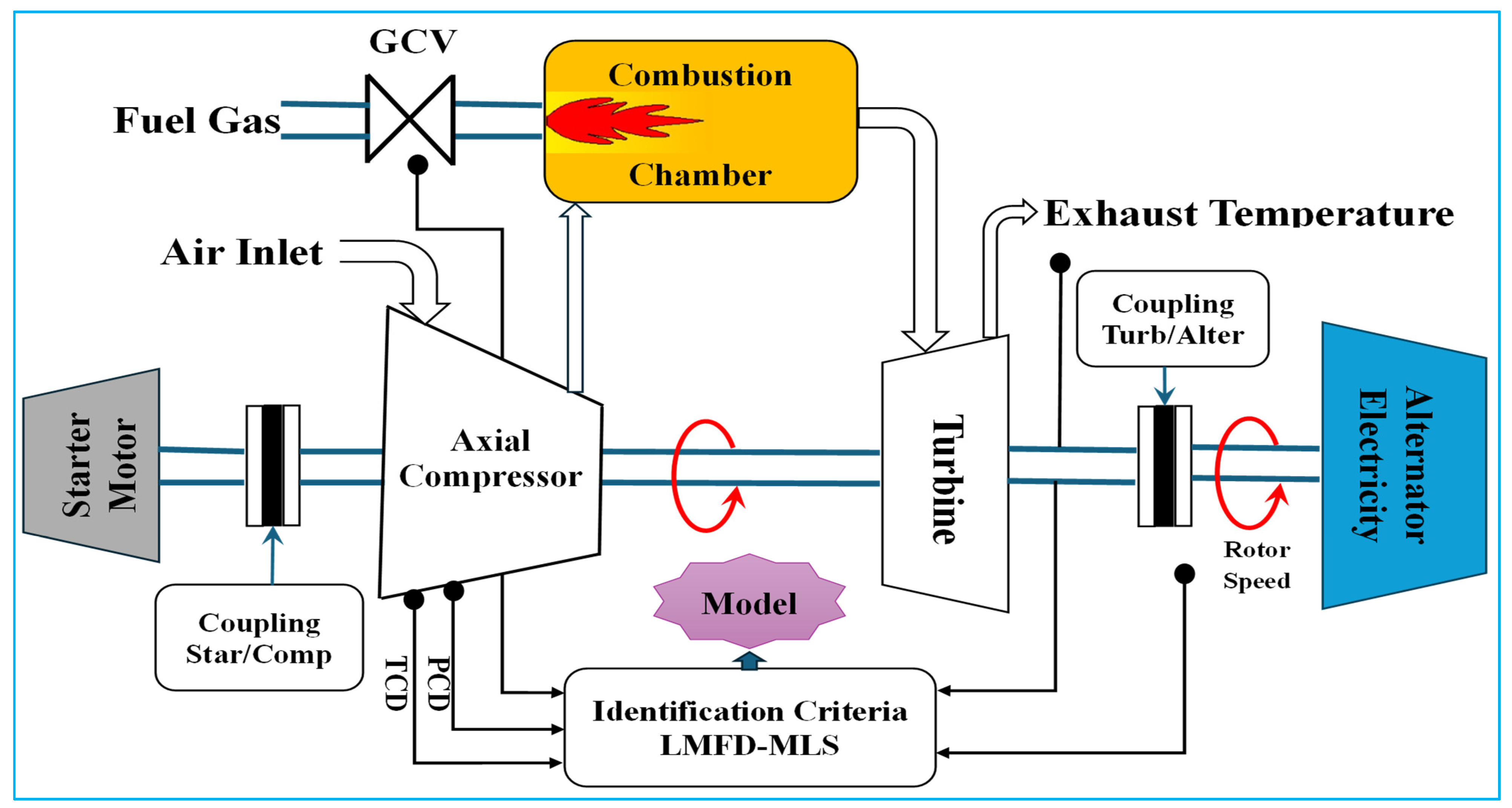
A schematic diagram for turbine identification is shown in Figure 2, illustrating the system inputs and outputs, the main components (axial compressor, combustion chamber, and turbine), and the electrical alternator as the load [31].
The following state-space representation models the gas turbine dynamics
    d d t x 1 x 2 x 3 x 4 x 5 x 6 = 0.32   0.10 0.18 0 0 0.35   0.15 0.45 0.25 0.30 0.15 0   0.10 0.30 0.60 0.20 0 0   0 0.20 0.15 0.55 0.30 0   0.18 0 0 0.25 0.50 0.20   0.25   0 0 0 0 0.65 x 1 x 2 x 3 x 4 x 5 x 6 + 0.60 0.50 0.20 0.80 0.70 0.90 0.10 0.30 0.40 0.15 0.20 0 u 1 u 2   y 1 y 2 = 1 0   0 0   0 0   0 0   0 1   0 0 x t + 0 0 0 0 u 1 u 2    
u 1 = G C V Gas control valve (fuel flow command);
u 2 = T C D r e f Compressor discharge temperature reference;
y 1 = ω r Rotor speed;
y 2 = T e Exhaust gas temperature.
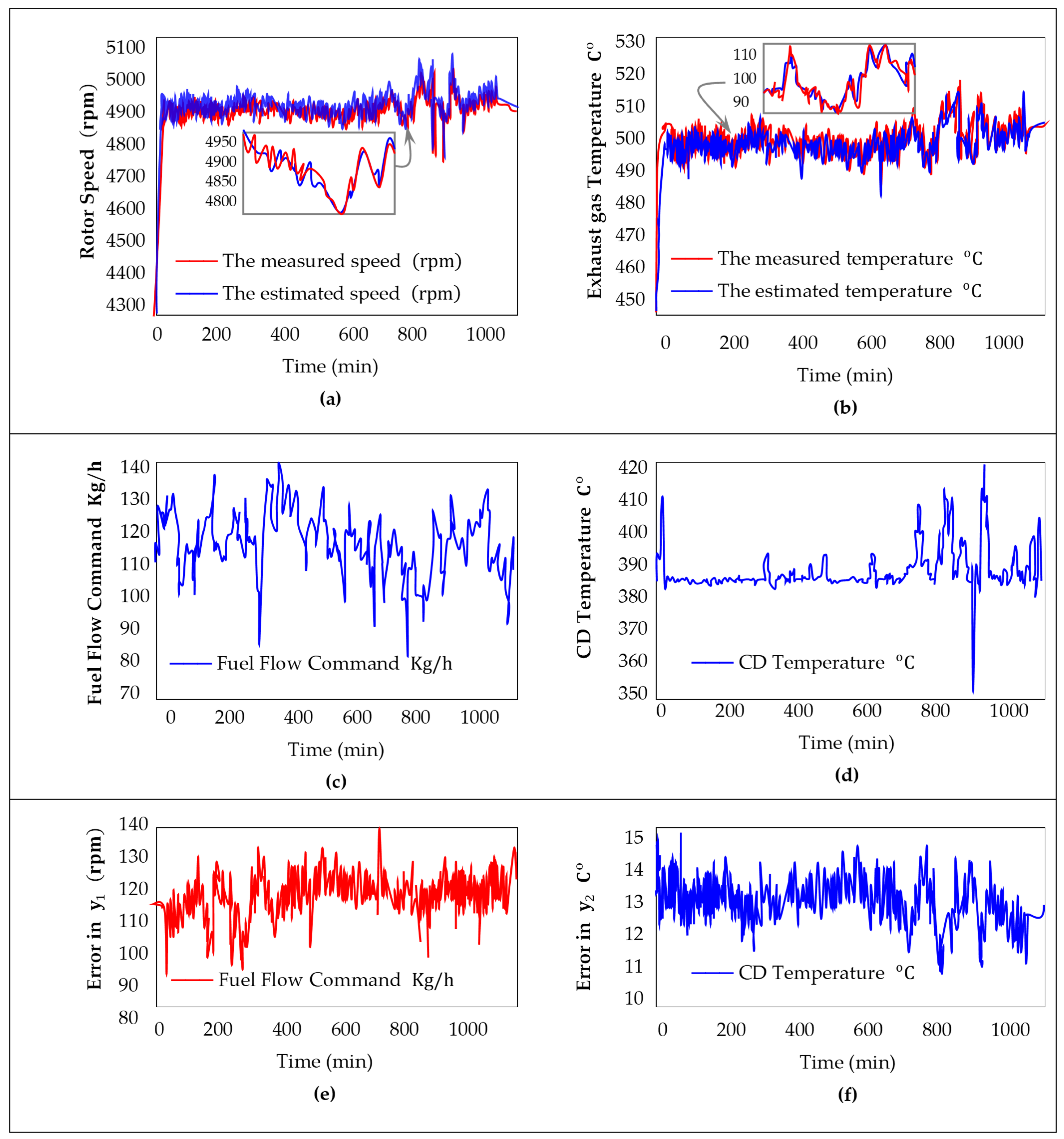
Physical Interpretation: Rotor speed is governed by shaft torque and turbine temperature, while compressor discharge temperature and pressure are strongly coupled, and exhaust temperature reflects combustion and turbine expansion dynamics. Shaft torque provides the link between thermal and mechanical subsystems. The GCV influences fuel flow, turbine temperature, torque, and speed, whereas the TCD reference regulates compressor and exhaust thermal states. Within this context, block controllability represents the ability to regulate these coupled mechanical–thermal subsystems through the available actuators. The identification results are evaluated by comparing the model-predicted outputs with the measured data. Figure 3 shows the temporal evolution of the input signals, the resulting state trajectories, and the corresponding outputs.
Figure 3 illustrates the temporal evolution of the system inputs, states, and outputs, together with the associated modeling errors. Specifically, Figure 3a compares the measured and estimated rotor speed y 1 = ω r , while Figure 3b presents the measured and estimated exhaust gas temperature y 2 = T e , showing a close agreement in both cases. The applied fuel flow command is depicted in Figure 3c, and the corresponding combustion chamber (TCD) temperature response is shown in Figure 3d. The modeling accuracy is further assessed through the error signals, defined as the difference between measured and estimated outputs, where Figure 3e shows the error in rotor speed y 1 and Figure 3f shows the error in exhaust gas temperature y 2 . As observed, the errors remain small over the entire operating range, indicating that the identified model accurately captures the system dynamics and provides a reliable basis for control design.
Table 2 shown below clarifies the change in the orders n until the best one is reached. From the results of this table, it can be concluded that the best model, which fits the minima of AICs, FPEs, RMSEs, the maximum of VAF validation criteria, and the minimum loss function without pole/zero cancelation (left coprime), is the model of order n   =   6 with number of blocks l = 3 .

4.3. Supervisory Control of the Gas Turbine Machine

In order to fulfill the main objective of this paper, the proposed algorithm is implemented on the studied system in accordance with the previously described steps.
The ratio l = n / m equals to 6 / 2 = 3 , it is an integer.
The block controllability matrix is satisfied as r a n k Ω c =   6 (full rank).
The transformation matrix T c R 6 × 6 is calculated by Equations (31)–(33).
Construct the desired right block roots such that V R is nonsingular.
Find the matrix coefficient N i and D i by Equations (34) and (35).
The feedback gain matrix K c is calculated based on (32) or (48).
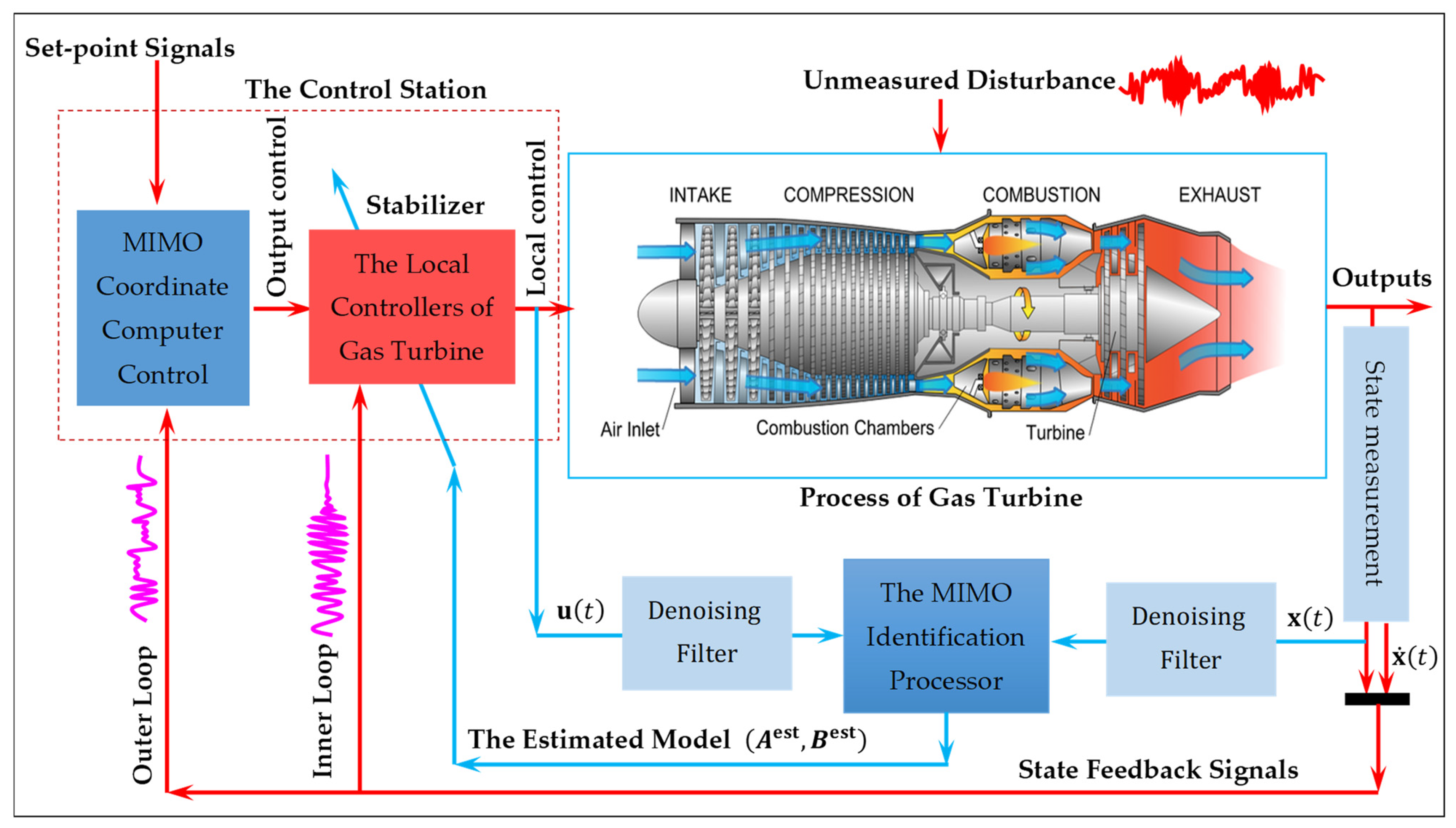
The overall supervisory control architecture, including the reference adjustment mechanism, is illustrated in Figure 4.
In recent years, various control strategies have been proposed for multivariable gas turbine systems, involving trade-offs between performance, robustness, and computational complexity. Robust and adaptive methods such as H∞ and sliding mode control effectively handle uncertainties and disturbances but often increase controller complexity and tuning sensitivity [29,30]. Model Predictive Control (MPC) provides systematic constraint handling and multi-objective optimization, yet its computational burden can limit real-time implementation for fast dynamics [32]. Matrix-based and linear algebraic approaches, including generalized eigenstructure assignment and block polynomial methods [27,36], are closely related to the present work through closed-loop pole assignment and structured state feedback, but typically assume full state availability or suffer from higher algebraic complexity in MIMO extensions. Observer-based schemes address state unavailability at the cost of added dynamics and noise sensitivity [37,38].
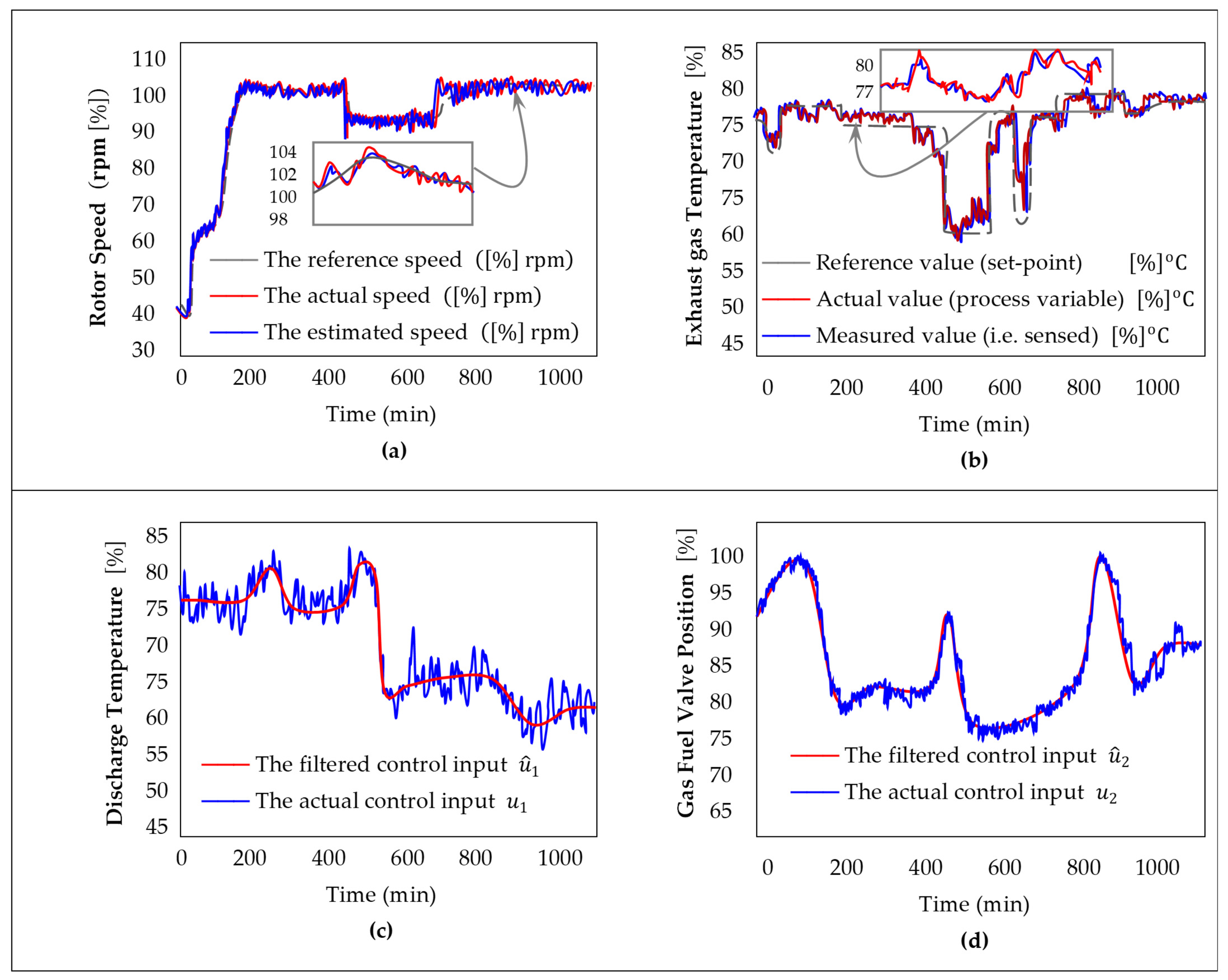
Figure 5 illustrates the dynamic response of the system variables and control inputs. Subplots (a) and (b) show the rotor speed and exhaust gas temperature, respectively, comparing the reference values (setpoints), actual values (process variables), and measured values obtained from sensors. Subplots (c) and (d) present the filtered control inputs alongside the actual control signals, demonstrating the effectiveness of the control strategy in tracking the references and maintaining system stability.
The proposed state-derivative feedback leverages the time derivatives of key mechanical and thermal states to enhance closed-loop performance. By incorporating derivative information, the controller improves damping, reduces overshoot, and accelerates transient response, particularly for rotor speed and shaft torque, which exhibit faster dynamics. In practical implementations, since direct measurement of state derivatives is often infeasible due to sensor limitations and noise sensitivity, the proposed approach relies on estimated derivatives obtained through adaptive filtering techniques that ensure accurate estimation while attenuating measurement noise. Compared to conventional state-feedback approaches, this method achieves superior stability and robustness while maintaining a low computational burden, making it well-suited for real-time control of industrial gas turbines. To demonstrate its effectiveness and advantages, a comparative study (Table 3) is conducted with classical and recent control strategies, including classical pole placement with stable eigenvalue assignment [39], discrete time linear quadratic regulator (DLQR) based on minimizing energy criteria [35], eigenstructure assignment with separate placement of eigenvalues and eigenvectors [36], stabilizing linear multivariable gas turbine model via sliding mode control [34], and the proposed linear algebraic state and state-derivative feedback method based on matrix polynomial theory, which simplifies implementation by directly leveraging measurable derivatives and ensures competitive pole placement capabilities.
The table compares the feedback gain norms ( K 1 , K 2 , K ) for different control methods applied to the gas turbine system. The proposed method and DLQR exhibit relatively low gain magnitudes, indicating moderate control effort and less aggressive feedback, while linear sliding mode shows the highest norms, reflecting stronger control action. Classical pole placement and Eigen-Structure Assignment lie in between, with Eigen-S having slightly higher norms due to the complexity of eigenvector shaping. Overall, the proposed state-derivative feedback achieves a good balance between performance and control effort.
Let λ i , v i and t i be the i t h eigenvalue, right and left eigenvectors of A , respectively, and let λ i + λ i be the i t h eigenvalue of A + A (i = 1, 2, …, n). Then, the eigenvalue sensitivity is defined as s λ i = t i   · v i λ i / A . The individual relative change in eigenvalues is r i = r λ i = | λ i | / | λ i | for i = 1, 2, …, n. Let λ i i = 1 n be the set of eigenvalues of an n × n matrix denoted by A and assuming that all the eigenvalues are stable R e λ i < 0 ,   i and have been arbitrarily assigned to guarantee performance. The three robust stability measures are defined by the following: M 1 = min ω [ 0   [ σ A j ω I where σ denotes the smallest singular value, and M 2 = min ω [ 0   [ κ 1 Λ · R e λ n in such a manner: R e λ n < < R e λ 1 , the matrix Λ R n × n is the diagonal form of A R n × n , and M 3 = min i 1   n s 1 λ i · R e λ i [7].
The sensitivity of the closed-loop eigenvalues with respect to perturbations in the system matrix is presented in Table 4, where the proposed method consistently exhibits lower sensitivity values compared to the other methods.
As shown in Table 5, the proposed method exhibits the smallest relative eigenvalue variations under perturbations while achieving the largest stability margins M 1 , M 2 , and M 3 , confirming its superior robustness performance.
From Table 4 and Table 5, it is observed that the proposed method yields significantly lower eigenvalue sensitivities s λ i and smaller relative variations r λ i under perturbations compared with the classical and recent control strategies. Moreover, the associated stability measures M 1 M 3 attain their highest values for the proposed approach, indicating improved robustness margins and enhanced tolerance to modeling uncertainties. Table 6 compares the settling time ( t s ) and maximum peak ( M p ) of each state for different control methods.
The proposed method achieves the fastest settling times and the lowest overshoots across all states, indicating superior transient response and damping. While DLQR and ES-assignment also show moderate improvements over pole placement, linear sliding mode reduces overshoot for some states but does not consistently outperform the proposed approach. Overall, the results highlight the effectiveness of the proposed state-derivative feedback in improving both speed of response and peak suppression.
Table 7 summarizes a qualitative comparison of the considered control methods in terms of gain norm, time-domain specifications, robust stability, and robust performance.
The results of the feedback gain matrix K , obtained by applying all the steps of the proposed state-derivative feedback algorithm, are compared with other control methods, including pole placement, DLQR, Eigen-Structure Assignment, and linear sliding mode. The comparison, summarized in Table 7, is performed under the same conditions, including identical initial state values, desired pole locations, and a consistent level of injected disturbances. The qualitative evaluation considers key criteria such as norms, time specifications, robust stability measures ( s λ i , M 1 , M 2 , M 3 ), and robust performance r λ i , highlighting the relative advantages of each method.

4.4. Interpretations of the Obtained Results

  • Table 3 presents the amplitudes of the feedback gain matrix K computed for the first, second, and ∞-norms using the four reference methods and the proposed state-derivative feedback method. It is evident that the proposed method and DLQR yield the lowest gain norms, indicating moderate control effort. However, DLQR shows inferior performance in terms of other characteristics. Therefore, the K matrix obtained via the proposed method provides high performance with minimal control energy.
  • The eigenvalue sensitivity results, following perturbations A in the dynamic matrix A , are reported in the tables above (Table 4). The proposed method demonstrates greater robustness to internal dynamic changes compared to the other methods.
  • The proposed method exhibits minimal relative change in eigenvalues, whereas other algorithms show significant variations that could potentially compromise system stability. Based on the defined stability measures and the obtained results (Table 5), the proposed algorithm consistently achieves the highest values for M 1 , M 2 and M 3 , particularly for M 1 , and M 3 , indicating superior stability performance.
  • Table 6 summarizes the time-domain specifications, including settling time ( t s ) and maximum peak ( M p ) for all states. The proposed method achieves the fastest settling times and lowest overshoots, which can be attributed to the diagonal assignment of robust block roots derived from the speed eigenvalues and eigenvectors.
  • Overall, the comprehensive comparison presented in Table 7 confirms that the proposed state-derivative feedback algorithm ensures the best combination of robust stability, transient performance, and eigenvalue sensitivity among all methods considered in this study.

4.5. Comments and Perspectives

A necessary condition for the proposed method to have block-root and block-vector assignment is the block controllability; if it is satisfied, then we may use the artificial control proposed by Malika Yaici [8].
In this work, the latent structure was arbitrarily chosen so that the block roots to be placed are arbitrary; hence, to meet specified objectives, some criterion should be explored to give the best desired block roots in order to improve the performance of the closed-loop system behavior.
In some systems, the full state is not available, and then one may think to explore and develop the problem of the block-structure assignment via state feedback to block-structure assignment via output feedback or feedback compensator design.
Latent structure assignment, which is the (block-roots, block-vectors) placement, provides a large degree of freedom in the design of the feedback gain matrix because the latent structure is more general and alters both the stability and the transient responses.
Many research works have been conducted on the specification of eigenvalues and eigenvectors for multivariable systems to achieve certain desired behavior or performance of the system, but there is no known latent structure specifications research using state and state derivative feedback via linear algebra theory and matrix polynomials.
Future research will focus on incorporating recent advances in gas turbine component design and manufacturing into control-oriented dynamic models. In particular, developments in integral blade rotor manufacturing, additive-manufactured burners, and topology-optimized centrifugal impellers demonstrate how modern fabrication techniques can significantly affect structural, thermal, and dynamic characteristics of gas turbines [40,41,42,43,44,45,46]. Accounting for these effects will enable the extension of the proposed linear algebra-based state-derivative feedback control framework to next-generation gas turbines, improving robustness and performance.
Future work should focus on developing and evaluating alternative system identification methods [47,48,49,50,51] to enhance the fidelity of control-oriented models. Particular attention is needed to address structural constraints within the modeling framework and to ensure robustness under limited excitation and measurement uncertainty. Improvements in model accuracy under practical operating conditions, including nonlinearities and parameter variations, are essential for reliable controller design and predictive performance.
Extending the experimental validation of state-derivative feedback remains a key area for further investigation [52,53,54,55]. This includes accurate derivative estimation under noisy measurements, assessment of actuator limitations and delays, and comprehensive evaluation of robustness beyond classical eigenvalue-based criteria. Developing methodologies that ensure performance in the presence of sensor noise, disturbances, and real-world operational constraints will be critical for transitioning these control strategies from laboratory to industrial applications.
The scalability of the proposed control framework to large-scale gas turbine systems warrants further exploration [56,57,58,59,60,61,62]. Future studies should assess computational efficiency and feasibility for high-dimensional models and complex real-time applications. In addition, extending the framework to modern gas turbines requires consideration of advanced manufacturing techniques, evolving structural dynamics, and digital-twin-based monitoring. Such efforts will facilitate the practical deployment of the methodology in industrial settings, enabling robust, efficient, and scalable control for next-generation gas turbine systems.

5. Conclusions

In this paper, a new state-derivative feedback control algorithm for a class of MIMO linear systems has been proposed, based on the assignment of block roots extracted from the dominant eigenvalues. The block roots are assigned diagonally and placed in the right block controllable form (right block Vandermonde matrix) of the transformed decomposed system using the feedback gain K . To validate the proposed method, the GE MS5001P gas turbine was selected due to its industrial importance, particularly in electrical power generation. The algorithm was applied to a real turbine model obtained from on-site experimental data, using parametric identification based on LMFD MIMO least squares. The robustness and stability of the proposed method were verified through stability measures, which demonstrated its effectiveness and validity. A comparative study with classical and recent control strategies clearly showed that the proposed algorithm provides superior performance, enhanced robustness, and improved transient response, highlighting the direct impact of block-root assignment on turbine operation. Consequently, this approach can be considered a promising solution for stability control in various industrial applications. The main limitations of the proposed algorithm are as follows:
  • The ratio n / m must be an integer; otherwise, other techniques can be employed.
  • The block controllability matrix must have full rank; otherwise, the algorithm is not applicable. Model order reduction can be used.
Future research can focus on optimal block root selection to reduce the norm of the feedback matrix K and minimize control energy. Additionally, the development of multivariable optimal static output-feedback controllers based solely on available outputs represents a promising direction for extending this work.

Author Contributions

B.B.: Conceptualization, methodology, software, formal analysis, investigation, data curation, original draft writing, visualization, and project administration; K.H. and A.G.: Supervision, validation, methodology, and review and editing of the manuscript; A.-N.S.: Visualization, formal analysis, methodology, data curation, validation, overall supervision, funding acquisition, project coordination, draft writing and critical manuscript revision. All authors have read and agreed to the published version of the manuscript.

Funding

This research received no external funding.

Data Availability Statement

The original contributions presented in this study are included in the article. Further inquiries can be directed to the corresponding author.

Conflicts of Interest

The authors declare no conflicts of interest.

Abbreviations

The following abbreviations are used in this manuscript:
DLQRDiscrete time linear quadratic regulator
ESAEigen-Structure Assignment
GCVGas control valve
LMFDLeft matrix fraction description
LQRLinear quadratic regulator
LTRLoop Transfer Recovery
MFDMatrix fraction description
MIMOMulti-Input Multi-Output
MPCModel Predictive Control
RMFDRight matrix fraction description
TCDTemperature of the Compressor Discharge
PCDPressure of the Compressor Discharge

Appendix A

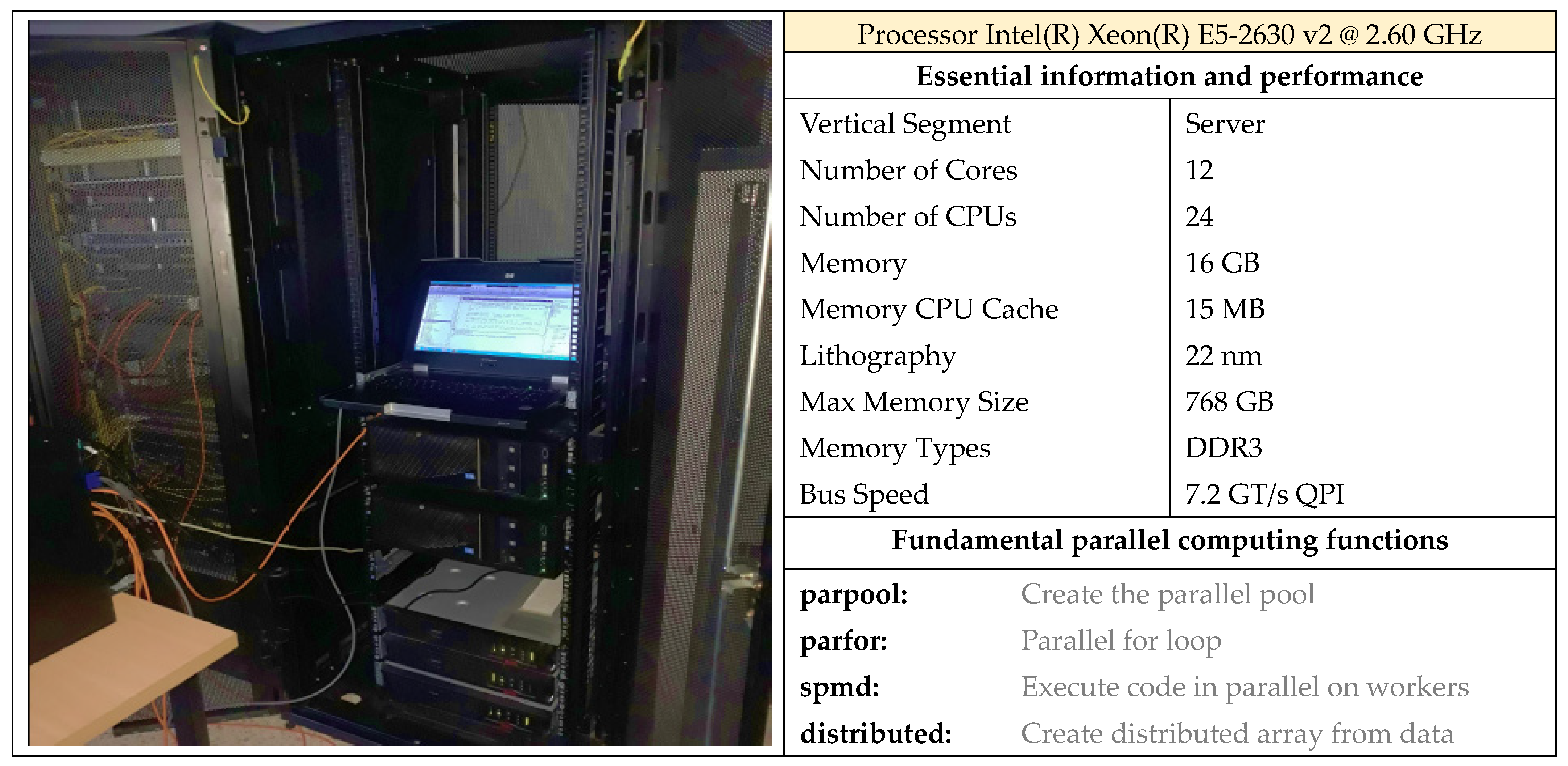
This appendix provides supplementary data supporting the numerical results obtained from the application of the state-derivative feedback controller, with particular emphasis on the computational platform used for optimization and parallel simulations. All simulations were performed on a high-performance server equipped with an Intel® Xeon® E5-2630 v2 processor operating at 2.60 GHz, featuring 12 physical cores and 24 logical processors for efficient parallel execution. The system includes 16 GB of RAM and a 15 MB shared CPU cache, ensuring adequate memory bandwidth and low-latency data access for large-scale numerical optimization. The 22 nm architecture and high-speed 7.2 GT/s QPI interconnect provide stable performance and scalability, with support for up to 768 GB of DDR3 memory for future expansion. Parallel computing tools such as parpool, parfor, spmd, and distributed arrays were employed to accelerate optimization routines and simulation workloads, enabling reliable evaluation of the proposed control strategy.
Machines 14 00169 g0a1

References

  1. Wonham, W.M. On pole assignment in multi-input controllable linear systems. IEEE Trans. Autom. Control 1967, 12, 660–665. [Google Scholar] [CrossRef]
  2. Moore, B.C. On the flexibility offered by state feedback in multivariable systems beyond closed loop eigenvalue assignment. IEEE Trans. Autom. Control 1976, 21, 689–692. [Google Scholar] [CrossRef]
  3. Roppenecker, G. Minimum norm output feedback design under specified eigenvalue areas. Syst. Control. Lett. 1983, 3, 101–103. [Google Scholar] [CrossRef]
  4. Fahmy, M.M.; O’Reilly, J. Eigenstructure Assignment in Linear Multivariable Systems-A Parametric Solution. IEEE Trans. Autom. Control. 1983, 28, 290–294. [Google Scholar] [CrossRef]
  5. Andry, A.N.; Shapiro, E.Y.; Chung, J.C. Eigenstructure assignment for linear systems. IEEE Trans. Aerosp. Electron. Syst. 1983, 19, 711–729. [Google Scholar] [CrossRef]
  6. Patel, R.V.; Misra, P. Numerical algorithms for eigenvalue assignment by state feedback. Proc. IEEE 1984, 72, 1755–1764. [Google Scholar] [CrossRef]
  7. Bekhiti, B. Multivariable Control System Design Using the Theory of Matrix Polynomials. Ph.D. Thesis, Boumerdes University Algeria, Boumerdès, Algeria, 2018. [Google Scholar]
  8. Yaici, M.; Hariche, K. On eigen-structure assignment using block poles placement. Eur. J. Control. 2014, 20, 217–226. [Google Scholar] [CrossRef]
  9. Bekhiti, B.; Hariche, K.; Zaitsev, V.; Duan, G.R.; Sharkawy, A.-N. The Algebraic Theory of Operator Matrix Polynomials with Applications to Aero-elasticity in Flight Dynamics and Control. Math. Comput. Appl. 2025, 30, 131. [Google Scholar] [CrossRef]
  10. Becher, D. Eigenvalue assignment by output-feedback with reduced sensor-actuator design. Mech. Syst. Signal Process. 2025, 241, 113372. [Google Scholar] [CrossRef]
  11. Siahlooei, E.; Fazeli, S.A.S.; Karbassi, S.M. Eigenvalue assignment via uncertain state feedback controllers. Asian J. Control 2019, 22, 1860–1869. [Google Scholar] [CrossRef]
  12. Duan, G.R. Solutions of the equation AV + BW = V F and their application to eigenstructure assignment in linear systems. IEEE Trans. Aut. Control 1993, 38, 276–280. [Google Scholar] [CrossRef]
  13. Sobel, K.M.; Shapiro, E.Y.; Andry, A.N. Eigenstructure Assignment. Int. J. Control 1994, 59, 13–37. [Google Scholar] [CrossRef]
  14. Liu, G.P.; Patton, R.J. Robust control design using eigenstructure assignment and multi-objective optimization. Int. J. Syst. Sci. 1996, 27, 871–879. [Google Scholar] [CrossRef]
  15. Bekhiti, B.; Al-Sabur, R.; Roudane, M.; Younis, J.A.; Sharkawy, A.-N. Intelligent neuro-fuzzy adaptive MIMO control for a self-balancing two wheeled autonomous robot via recursive resolution of the matrix Diophantine equation. Discov. Robot. 2025, 1, 11. [Google Scholar] [CrossRef]
  16. Liu, G.P.; Patton, R.J. Eigenstructure Assignment for Control System Theory; John Wiley & Sons: Hoboken, NJ, USA, 1998; pp. 55–122. [Google Scholar]
  17. Patton, R.J.; Liu, G.P. Robust control design via eigenstructure assignment, genetic algorithms and gradient-based optimization. IEEE Proc. Control. Theory Appl. 1994, 141, 202–208. [Google Scholar] [CrossRef]
  18. Bekhiti, B.; Fragulis, G.F.; Maraslidis, G.S.; Hariche, K.; Cherifi, K. A Novel Recursive Algorithm for Inverting Matrix Polynomials via a Generalized Leverrier–Faddeev Scheme: Application to FEM Modeling of Wing Vibrations in a 4th-Generation Fighter Aircraft. Mathematics 2025, 13, 2101. [Google Scholar] [CrossRef]
  19. Shieh, L.S.; Tsay, Y.T.; Coleman, N.I. Algorithms for solvents and spectral factors of matrix polynomials. Int. J. Control 1981, 12, 1303–1316. [Google Scholar] [CrossRef]
  20. Bachelier, O.; Mehdi, D. Non-iterative pole placement technique: A step further. J. Frankl. Inst. 2008, 345, 267–281. [Google Scholar] [CrossRef]
  21. Karbassi, S.M.; Saadatjou, F. A parametric approach for eigenvalue assignment by static output feedback. J. Frankl. Inst. 2009, 346, 289–300. [Google Scholar] [CrossRef]
  22. Bekhiti, B.; Hariche, K.; Kouzou, A.; Younis, J.A.; Sharkawy, A.-N. On Matrix Linear Diophantine Equation-Based Digital-Adaptive Block Pole Placement Control for Multivariable Large-Scale Linear Process. AppliedMath 2025, 5, 139. [Google Scholar] [CrossRef]
  23. Pereira, E. On solvents of matrix polynomials. Appl. Numer. Math. 2003, 47, 197–208. [Google Scholar] [CrossRef]
  24. Bekhiti, B.; Hariche, K.; Iqbal, J.; Sharkawy, A.N. Parametric Eigen-space Characterization via Static Output Feedback in MIMO Control Systems: A New Look to Output Feedback Gain Matrix Design for Turbo-Generator System. Int. J. Robot. Control. Syst. 2025, 5, 2546–2567. [Google Scholar] [CrossRef]
  25. Periera, E. Block eigenvalues and solution of diff-matrix equation. Math. Notes 2003, 4, 45–51. [Google Scholar] [CrossRef]
  26. Zhang, B. Parametric Eigenstructure Assignment for Descriptor Systems via Proportional plus Derivative State Feedback. Int. J. Control. Autom. Syst. 2011, 9, 15–22. [Google Scholar] [CrossRef]
  27. Bekhiti, B.; Hariche, K.; Fragulis, G.F.; Sharkawy, A.-N. Matrix Fraction Description in Large Scale MIMO Descriptor Systems: Matrix Polynomials Approaches. Symmetry 2025, 17, 1413. [Google Scholar] [CrossRef]
  28. Bagua, H.; Hafaifa, A.; Iratni, A.; Guemana, M. Model variables identification of a gas turbine using a subspace approach based on input/output data measurements. Control. Theory Technol. 2021, 19, 183–196. [Google Scholar] [CrossRef]
  29. Bianco, S.J. Sliding Mode Transient Scaling Controller for Gas Turbine Engine Emulation on an Electric Machine. In Proceedings of the AIAA 2020-3677. Session: Software Systems and Modeling for Electrified Propulsion, Virtual, 24–28 August 2020. [Google Scholar] [CrossRef]
  30. Biss, D.; Woodgate, K.G. Gas Turbine Control Using Mixed Sensitivity H∞-Optimisation. In Robust Control of Linear Systems and Nonlinear Control: Progress in Systems and Control Theory; Kaashoek, M.A., van Schuppen, J.H., Ran, A.C.M., Eds.; Birkhäuser: Boston, MA, USA, 1990; Volume 4. [Google Scholar] [CrossRef]
  31. Bonfiglio, A.; Cacciacarne, S.; Invernizzi, M.; Lanzarotto, D.; Palmieri, A.; Procopio, R. A Sliding Mode Control Approach for Gas Turbine Power Generators. IEEE Trans. Energy Convers. 2019, 34, 921–932. [Google Scholar] [CrossRef]
  32. Hou, G.; Gong, L.; Yang, Z.; Zhang, J. Multi-objective economic model predictive control for gas turbine system based on quantum simultaneous whale optimization algorithm. Energy Convers. Manag. 2020, 207, 112498. [Google Scholar] [CrossRef]
  33. Palmieri, A.; Lanzarotto, D.; Cacciacarne, S.; Torre, I.; Bonfiglio, A. An Innovative Sliding Mode Load Controller for Gas Turbine Power Generators: Design and Experimental Validation Via Real-Time Simulation. Energy 2021, 217, 119363. [Google Scholar] [CrossRef]
  34. Nail, B.; Kouzou, A.; Hafaifa, A.; Bekhiti, B. Stabilizing linear multivariable gas turbine model via sliding mode control. Fundam. Sci. Appl. 2016, 22, 25–30. [Google Scholar]
  35. Shabaninia, F.; Jafari, K. Using LQG/LTR Optimal Control Method to Improve Stability and Performance of Industrial Gas Turbine System. Int. Sch. Res. Netw. ISRN Electron. 2012, 2012, 134580. [Google Scholar] [CrossRef]
  36. Abdellah, K. Block pole assignment stabilization in large scale systems: Application to gas turbine power plant. In Proceedings of the International Conference on Technological Advances in Electrical Engineering ICTAEE’16, Skikda, Algeria, 24–26 October 2016. [Google Scholar]
  37. Simani, S.; Spina, P.R. Kalman Filtering to Enhance the Gas Turbine Control Sensor Fault Detection. Theory Pract. Control. Syst. 1999, 443–450. [Google Scholar] [CrossRef]
  38. Ahmed, J.M. Optimal tuning linear quadratic regulator for gas turbine by genetic algorithm using integral time absolute error. Int. J. Electr. Comput. Eng. 2020, 10, 1367. [Google Scholar] [CrossRef]
  39. Sarjaš, A.; Chowdhury, A.; Svečko, R. Robust Optimal Regional Closed-loop Pole Assignment over Positivity Conditions and Differential Evolution. IFAC PapersOnLine 2015, 48, 141–146. [Google Scholar] [CrossRef]
  40. González-Barrio, H.; Calleja-Ochoa, A.; Lamikiz, A.; de Lacalle, L.N.L. Manufacturing Processes of Integral Blade Rotors for Turbomachinery, Processes and New Approaches. Appl. Sci. 2020, 10, 3063. [Google Scholar] [CrossRef]
  41. Cascino, A.; Meli, E.; Rindi, A.; Pucci, E.; Matoni, E. Experimental Validation and Dynamic Analysis of Additive Manufacturing Burner for Gas Turbine Applications. Machines 2025, 13, 1111. [Google Scholar] [CrossRef]
  42. Liu, S.; Mi, D.; Wen, C.; Zheng, Y. Topology Optimization Design With Addictive Manufacturing Constraints for Centrifugal Impeller. J. Phys. Conf. Ser. 2022, 2252, 012026. [Google Scholar] [CrossRef]
  43. Adamou, A.; Turner, J.; Costall, A.; Jones, A.; Copeland, C. Design, simulation, and validation of additively manufactured high-temperature combustion chambers for micro gas turbines. Energy Convers. Manag. 2021, 248, 114805. [Google Scholar] [CrossRef]
  44. Zajadatz, M.; Güthe, F.; Freitag, E.; Ferreira-Providakis, T.; Wind, T.; Magni, F.; Goldmeer, J. Extended Range of Fuel Capability for GT13E2 AEV Burner With Liquid and Gaseous Fuels. J. Eng. Gas Turbines Power 2018, 141, 051017. [Google Scholar] [CrossRef]
  45. Remache, A.; Pérez-Sánchez, M.; Hidalgo, V.H.; Ramos, H.M. Hybrid Optimization Approaches for Impeller Design in Turbomachinery: Methods, Metrics, and Design Strategies. Water 2025, 17, 1976. [Google Scholar] [CrossRef]
  46. Meli, E.; Furferi, R.; Rind, A.; Ridolfi, A.; Volpe, Y.; Buonamici, F. A General Framework for Designing 3D Impellers Using Topology Optimization and Additive Manufacturing. IEEE Access 2020, 8, 60259–60269. [Google Scholar] [CrossRef]
  47. Yang, R.; Liu, Y.; He, X.; Liu, Z. Gas Turbine Model Identification Based on Online Sequential Regularization Extreme Learning Machine with a Forgetting Factor. Energies 2023, 16, 304. [Google Scholar] [CrossRef]
  48. Villarreal-Valderrama, F.; Liceaga-Castro, E.; Hernandez-Alcantara, D.; Santana-Delgado, C.; Ekici, S.; Amezquita-Brooks, L. Control-oriented system identification of turbojet dynamics. Aerospace 2024, 11, 630. [Google Scholar] [CrossRef]
  49. Sadjadi, E.N.; Garcia, J.; Lopez, J.M.M.; Borzabadi, A.H.; Abchouyeh, M.A. Fuzzy Model Identification and Self Learning with Smooth Compositions. Int. J. Fuzzy Syst. 2019, 21, 2679–2693. [Google Scholar] [CrossRef]
  50. Wang, Q.-G.; Zhang, L. System Identification in the Network Era: A Survey of Data Issues and Innovative Approaches. IEEE CAA J. Autom. Sin. 2025, 12, 1305–1319. [Google Scholar] [CrossRef]
  51. Ma, S.; Wu, Y.; Hua, Z.; Gou, L. Application of Fuzzy Inference System in Gas Turbine Engine Fault Diagnosis Against Measurement Uncertainties. Chin. J. Mech. Eng. 2025, 38, 2. [Google Scholar] [CrossRef]
  52. Wen, D.; Sun, C.; Huang, S.; Yi, S. Robust fault estimation and proportional derivative fault tolerant control for a class of singular systems with interval time-varying delay and disturbance. Optim. Control. Appl. Methods 2024, 45, 928–953. [Google Scholar] [CrossRef]
  53. Sariyildiz, E.; Yu, H.; Ohnishi, K. A Practical Tuning Method for the Robust PID Controller with Velocity Feed-Back. Machines 2015, 3, 208–222. [Google Scholar] [CrossRef]
  54. Yu, P.; Wan, H.; Zhang, B.; Wu, Q.; Zhao, B.; Xu, C.; Yang, S. Review on System Identification, Control, and Optimization Based on Artificial Intelligence. Mathematics 2025, 13, 952. [Google Scholar] [CrossRef]
  55. Yessef, M.; Benbouhenni, H.; Lagrioui, A.; Bizon, N.; Bossoufi, B.; Al-Gahtani, S.F.; Elbarbary, Z.M.S. Processor-in-the-Loop validation of direct power control based on fractional-order modified super-twisting algorithm for doubly-fed induction generators. Sci. Rep. 2025, 15, 22846. [Google Scholar] [CrossRef]
  56. Aquize, R.; Cajahuaringa, A.; Machuca, J.; Mauricio, D.; Villanueva, J.M.M. System Identification Methodology of a Gas Turbine Based on Artificial Recurrent Neural Networks. Sensors 2023, 23, 2231. [Google Scholar] [CrossRef]
  57. Wang, R.; Hu, J.; Xin, D.; Liu, S.; Zhao, K. Robust subspace tracking in intelligent fault diagnosis of digital twin gas turbines base on the adaptive Markov transfer. Appl. Energy 2025, 401, 126747. [Google Scholar] [CrossRef]
  58. Pedroso, L.; Batista, P.; Heemels, W. Distributed design of ultra-large-scale control systems: Progress, Challenges, and Prospects. Annu. Rev. Control. 2025, 59, 100987. [Google Scholar] [CrossRef]
  59. Farhat, H.; Altarawneh, A. Physics-Informed Machine Learning for Intelligent Gas Turbine Digital Twins: A Review. Energies 2025, 18, 5523. [Google Scholar] [CrossRef]
  60. Bruni, G.; Maleki, S.; Krishnababu, S.K. Deep learning modeling of manufacturing and build variations on multistage axial compressors aerodynamics. Data Centric Eng. 2025, 6, e9. [Google Scholar] [CrossRef]
  61. Zhang, J.; Wang, Z.; Li, S.; Wei, P. A digital twin approach for gas turbine performance based on deep multi-model fusion. Appl. Therm. Eng. 2024, 246, 122954. [Google Scholar] [CrossRef]
  62. Lim, J.T.; Habibullah, A.; Ng, E.Y.K. Towards a Digital Twin for Gas Turbines: Thermodynamic Modeling, Parameter Estimation, and Performance Optimization using PINN and PSO. Energies 2025, 18, 3721. [Google Scholar] [CrossRef]
Figure 1. GE 5001P gas turbine components: (a) axial compressor; (b) turbine.
Machines 14 00169 g001
Figure 2. Schematic overview of the GE MS5001P gas turbine illustrating its parts.
Machines 14 00169 g002
Figure 3. Measured outputs against model outputs and states with small prediction errors.
Machines 14 00169 g003
Figure 4. Supervisory control scheme incorporating reference adjustment.
Machines 14 00169 g004
Figure 5. Responses and control inputs, showing reference, actual, and measured values.
Machines 14 00169 g005
Table 1. General performance of gas turbine GE MS5001P.
QuantityValue QuantityValue
Compressor stages 16Output 24,700 (kW)
Firing temperature 1730 ( ° F )Heat rate 12,950 (kJ/kW-h)
Exhaust temperature 898 ( ° F ) Rotor Speed 5355 (rpm) (105%)
Air flow 928.5 (103 Lb/h)Efficiency27.8%
Table 2. Gas turbine system model orders with validations criteria, respectively.
LMFD ARX Model
l n Loss FunAICFPERMSEVAF (%)
125.43851.72005.58265.235482.5000
241.99670.74452.10245.457385.9050
361.02630.13191.13501.821787.7750
481.10450.17891.19234.720087.6550
Table 3. The norms (1, 2, inf) of the feedback gain matrix K associated with each method.
Method K 1 K 2 K
Pole placement [39]35.12043.50080.900
DLQR [35]21.85030.467477.2140
Eigen-S Assignment [36]37.132545.725394.2423
Linear Sliding Mode [34]65.015677.6217114.1543
Proposed Method 22.415031.421375.8065
Table 4. Robust stability (eigenvalues sensitivity s λ i ).
Method s λ 1 s λ 2 s λ 3 s λ 4 s λ 5 s λ 6
Pole Placement [39]213.0689213.0689129.667095.5432524.5128524.5128
Discrete-LQR [35]31.9535262.7456262.7456 1.8277 × 10 3 1.835 × 10 3 54.6149
Eigen-Structure Assignment [36]28.1816201.5546118.131592.1314403.678170.1324
Linear Sliding Mode [34]27.3356197.5478115.045690.4378 450.607170.8843
Proposed Method 12.728691.005291.005228.454081.451383.3787
Table 5. Robust performance (relative change r in the eigenvalues λ i under perturbation).
Method Relative   Change   in   λ i Under Perturbation Stability Measures
r λ 1 r λ 2 r λ 3 r λ 4 r λ 5 r λ 6 M 1 M 2 M 3
P-placement [39]1.3031.2011.6570.8501.3171.606 0.2725 × 10 5 0.1337 × 10 5 0.1438 × 10 5
D-LQR [35] 8.12 × 10−40.0180.0190.1150.1160.091 0.8220 × 10 4 0.3989 × 10 3 0.4289 × 10 4
ES Method [36] 8.01 × 10−40.0110.0170.1000.1240.082 0.2316 × 10 3 0.1124 × 10 3 0.1208 × 10 3
LS Mode [34] 7.953 × 10−40.0110.0980.0590.0690.069 0.2659 × 10 3 0.1290 × 10 3 0.1387 × 10 3
Proposed 7.526 × 10−40.0030.0030.0020.0100.002 0.230 × 10 2 0.1116 × 10 2 0.1200 × 10 2
Table 6. Time domain specifications (settling time t s and the maximum peak M p ).
Method x 1 x 2 x 3 x 4 x 5 x 6
Pole Placement [39] t s 606062626262
M p 73.4124143.6067275.8774480.030263.8776245.0559
Discrete-LQR [35] t s 403751504651
M p 32.322061.596035.979582.420036. 447872.6120
Eigen-Structure Assignment [36] t s 393845424039
M p 28.444056.375030.956075.526032.65465.4120
Linear Sliding Mode [34] t s 40393038 4240
M p 27.452050.898028.779568.325031.457664.8120
Proposed Method t s 373728373635
M p 15.736730.43028.644225.396911.310726.7737
Table 7. Qualitative evaluation of different control strategies for the gas turbine system.
Pole Placement [39]Discrete-LQR
[35]
Eigen-Structure Assignment [36]Linear Sliding Mode [34]Proposed Method
NormAcceptable ExcellentPoorPoorGood
Time specificationsPoorPoorAcceptableGoodExcellent
Robust stability s λ i PoorPoorGoodAcceptableExcellent
M 1 PoorePoorAcceptableAcceptableExcellent
M 2 PoorAcceptableAcceptableAcceptableExcellent
M 3 PoorPoorAcceptableAcceptableExcellent
Robust performance r λ i PoorGoodGoodGoodExcellent
Disclaimer/Publisher’s Note: The statements, opinions and data contained in all publications are solely those of the individual author(s) and contributor(s) and not of MDPI and/or the editor(s). MDPI and/or the editor(s) disclaim responsibility for any injury to people or property resulting from any ideas, methods, instructions or products referred to in the content.