Abstract
AI-integrated robotics in Industry 5.0 demands advanced manufacturing systems capable of autonomously interpreting complex geometries and dynamically adjusting machining strategies in real time—particularly when dealing with aerospace components featuring large-curvature surfaces. Large-curvature aerospace components present significant challenges for precision drilling due to surface-normal deviations caused by curvature, roughness, and thin-wall deformation. This study presents a robotic drilling system that integrates adaptive PCA-based surface normal estimation with in-process pre-drilling correction and post-drilling verification. This system integrates a 660 nm wavelength linear laser projector and a 1.3-megapixel industrial camera arranged at a fixed 30° angle, which project and capture structured-light fringes. Based on triangulation, high-resolution point clouds are reconstructed for precise surface analysis. By adaptively selecting localized point-cloud regions during machining, the proposed algorithm converts raw measurements into precise normal vectors, thereby achieving an accurate solution of the normal direction of the surface of large curvature parts. Experimental validation on a 400 mm-diameter cylinder shows that using point clouds within a 100 mm radius yields deviations within an acceptable range of theoretical normals, demonstrating both high precision and reliability. Moreover, experiments on cylindrical aerospace-grade specimens demonstrate normal direction accuracy ≤ 0.2° and hole position error ≤ 0.25 mm, maintained across varying curvature radii and roughness levels. The research will make up for the shortcomings of existing manual drilling methods, improve the accuracy of hole-making positions, and meet the high fatigue service needs of aerospace and other industries. This system is significant in promoting the development of industrial automation and improving the productivity of enterprises by improving drilling precision and repeatability, enabling reliable assembly of high-curvature aerospace structures within stringent tolerance requirements.
1. Introduction
With the advent of Industry 5.0, the integration of artificial intelligence (AI) into robotic systems has become essential for developing smart, human-centric, and adaptive manufacturing solutions [1]. In aerospace manufacturing, this paradigm translates into advanced robotic platforms capable of autonomously interpreting surface geometries, adjusting tool orientations, and verifying hole quality to ensure high assembly precision. Robotic drilling, in particular, plays a critical role in the assembly of fuselage sections, wings, and other components that require thousands of high-quality fastener holes.
In modern manufacturing systems, machine tools equipped with advanced in-process sensing and data-driven control algorithms are critical for delivering the precision, reliability, and automation required to produce complex, large-curvature components [2,3]. Aerospace manufacturing sits at the forefront of precision engineering, combining advanced materials science, high-tech production methods, and stringent quality control to deliver machines for satellites, launch vehicles, and inertial navigation systems [4]. Every hole, slot, and surface finish must meet micrometer-level tolerances to ensure structural integrity, aerodynamic performance, and fatigue life under extreme service conditions [5].
The application of aerospace technology in military, economic, communication, and other fields has significantly enhanced the comprehensive national strength of the country [6]. For example, technologies such as satellite reconnaissance and missile warning provide strong guarantees for maintaining national security, while technologies such as meteorological forecasting, resource exploration, and communication network construction inject new vitality into economic development [7]. The development of the aerospace industry is also related to the country’s economy and national defense security. Influenced by the rapid changes of modern science and technology, aviation products have evolved from singular to diverse, placing higher demands on production and assembly [8].
Traditional aviation assembly is mainly completed manually or with the help of tools [9]. The general steps include marking, hole-making, expanding, reaming, trimming, deburring, etc. Traditional aviation assembly faces multiple challenges: slow operation speed, low efficiency, and high cost, making it particularly difficult to achieve batch operations when handling large components [10]. In addition, there are various safety hazards hidden in the working environment of aviation assembly sites, which pose a threat to the safety of operators [11]. Therefore, it is crucial to adopt advanced assembly processes to transform from traditional manual assembly to automation and intelligence [12]. Among them, the perpendicularity of the connecting hole has a significant effect on the maximum tensile force of the connecting piece, which is an important indicator that needs to be strictly controlled in the aerospace manufacturing process. If the axis of the hole is not perpendicular to the surface of the workpiece, it will cause deformation of the connector, thereby reducing its fatigue life and even endangering flight safety and service life [13].
Driven by new-generation information technology and various emerging technologies, the aerospace manufacturing industry is gradually transitioning towards intelligence and digitization, entering a new development stage in Industry 5.0. In response to the complex resin distribution network in aviation composite materials, Szarski and Chauhan built a 3D finite element resin flow model for dry carbon preforms based on reinforcement learning. The model provided a good flow medium layout. The results showed that this method reduced filling time by 32% while maintaining the same filling quality [14]. To improve accuracy and reliability in aerospace manufacturing processes, Ruiz et al. built a Convolutional Neural Network (CNN) for detecting and measuring drill bits and other fixed components in uncontrolled industrial manufacturing environments. Through practical verification, the accuracy of this method was 99.7%, and the reduction rate of worker intervention decreased from 13.3% to 0.6% [15].
Herzog et al. built a defect detection strategy on the ground of machine learning for defects caused by the highly dynamic nature of laser technology in aerospace metal parts manufacturing. Sensing technologies and their applications in the monitoring task of laser metal additive manufacturing were compared [16]. In order to effectively suppress chatter during the milling process of thin-walled parts in aerospace manufacturing, Zhou et al. proposed a digital twin model, which used real-time stable blade plots with time-varying modal parameters as optimization criteria. The vibration, force, and sound signals from multiple sensors were fused and analyzed to identify flutter. Experimental results showed that this method effectively identified chatter during milling processes [17]. Zhu et al. built a machine learning strategy for process state monitoring in order to reduce various defects in aerospace metal-based additive manufacturing processes. By learning historical data, a correlation model between the production process and product quality was established to optimize parameter settings and improve product quality and production efficiency [18].
Machine vision positioning is widely used in the fields of automation and robotics, which can achieve automated assembly, precision control, and real-time detection, thereby improving the quality and efficiency of aircraft assembly and reducing human errors. In order to improve the positioning accuracy in aerospace parts manufacturing, Lin et al. built a visual interactive network topology model on the basis of real-time space flight features. The reconstructed point cloud data was reconstructed into Poisson surfaces. New model scene pages were quickly generated on the basis of the task characteristics, achieving 3D reconstruction of non-cooperative targets [19].
Fan et al. proposed a pose measurement approach for large aerospace components on the basis of binocular vision and prior data to achieve pose perception. The method used deep learning and prior processing data to match the 3D reconstruction coordinates of key feature centroids, which could calculate the spatial pose of aerospace components [20]. Simonov et al. proposed a cone beam X-ray computed tomography three-dimensional image reconstruction algorithm to control the additive manufacturing defect rate of high-reliability and expensive metal products in aerospace. By analyzing these scanned images, the internal structure of the manufacturing layer of the product at any point within its volume was determined [21].
Takahashi et al. used computer tomography background schlieren technique to reconstruct the three-dimensional flow field around a hypersonic aircraft model. The rotating model was used to obtain a projection image dataset, and reconstruction methods such as telecentric optical structure and filtered backprojection were employed. Combined with denoising calculations, a complex three-dimensional flow field was successfully reconstructed, visualizing dynamic physical features such as oblique shock waves [22]. Zhao et al. proposed a monocular depth estimation network that combined CNN and visual transformers to calculate the relative position between non-cooperative spacecraft and spacecraft. This network accurately estimated the global depth while preserving details [23].
Despite the progress in robotic drilling and vision-based positioning, a major technological gap remains in ensuring high-precision normal estimation on large single-curvature or double-curvature aerospace components. While industrial robots offer flexibility, their positioning accuracy (typically 0.1–0.3 mm) is inferior to that of dedicated Computer Numerical Control (CNC) machines, which complicates precision hole-making under demanding aerospace tolerances [24]. Similarly, the accuracy of industrial cameras and optical scanners is influenced by factors such as resolution, lens distortion, and calibration errors [25], which are seldom considered in integrated drilling systems. Most existing studies [14,19,20] emphasize 3D vision or offline calibration but fail to address the real-time normal deviation caused by surface roughness, curvature, and thin-wall deformation during drilling. Accurate normal estimation is the central challenge, as any angular misalignment between the drill axis and the surface normal generates additional bending stress on the fasteners, leading to reduced possible structural failure [5].
This study differs from existing approaches by integrating line structured-light sensing, adaptive Principal Component Analysis (PCA)-based normal fitting, and pre-/post-drilling quality verification into a single robotic drilling system. While vision-guided robotic drilling systems have been widely explored, most prior works focus on standard pose estimation, offline calibration, or fixed-radius PCA methods. These approaches do not address real-time adaptation to curvature-induced deviations or verify drilling accuracy in-process. The novelty of this work lies in combining adaptive PCA-based surface normal estimation with integrated pre- and post-drilling verification, enabling sub-millimeter positional accuracy and angular deviations within 0.2°, even on challenging large-curvature aerospace components.
Moreover, unlike conventional methods that rely solely on offline measurements or manual adjustments, our method performs both normal adjustment before drilling and dimensional quality checks after drilling, ensuring hole perpendicularity and position accuracy within sub-millimeter tolerance even on complex curved surfaces. The robotic hole-making system proposed in this study reflects this Industry 5.0 paradigm by combining machine vision, structured light sensing, and AI-driven normal estimation to ensure precision drilling on complex surfaces.
Research Gaps, Aims, and Contributions
Robotic hole-making on aerospace components faces unique challenges due to the thin-walled, single-curvature structures commonly used in fuselage panels and arc-shaped frames. While machine vision has been applied for pose estimation and 3D reconstruction [18,19,20], the integration of surface normal estimation with drilling accuracy verification remains underexplored. Additionally, the literature does not sufficiently address how machining constraints such as cutting forces, surface roughness, and thin-wall deformation affect hole quality [14,16,17]. For example, thin-walled aerospace parts tend to deform under drilling loads, which leads to misalignment of holes and reduced structural integrity. Moreover, there is limited research on real-time compensation for drilling-induced deflection in combination with vision-guided normal calculation. Moreover, this study aims to achieve the following:
- (1)
- Develop a vision-integrated robotic drilling system that combines line structured-light sensing with PCA-based normal vector estimation, tailored for single-curvature aerospace components.
- (2)
- Investigate the impact of surface roughness and curvature radius on normal estimation accuracy, which is often neglected in prior works.
- (3)
- Propose a pre-drilling and post-drilling quality verification algorithm that ensures the correct orientation of the drilling tool and checks hole dimensional accuracy after drilling.
Based on the above discussion, the key contributions of this work are:
- (1)
- A point-cloud-based normal estimation method with adaptive extraction and PCA plane fitting that achieves normal direction accuracy ≤ 0.2° on surfaces with curvature radii up to 50 mm and roughness ≤ Ra4.8.
- (2)
- A robotic drilling platform that achieves sub-millimeter hole position accuracy (0.08–0.25 mm), which meets the positional and angular requirements for aerospace assembly.
- (3)
- A dual-function algorithm for pre-adjusting the drilling normal and post-process inspection, ensuring that deviations in hole position and verticality remain within the target tolerance range.
- (4)
- The study also quantifies the relative influence of surface roughness and curvature radius on normal fitting error, demonstrating that curvature is the dominant factor impacting drilling precision.
2. Robot Automated Hole-Making Technology Driven by Artificial Intelligence in Aerospace Manufacturing
The study first comprehensively introduces the overall scheme of the automatic drilling system. Then, to ensure the accuracy and stability of the robot’s automatic hole-making system, a series of calibration work is carried out. Finally, a high-precision normal vector solving algorithm for large single-curvature surfaces is designed to provide support for robot hole-making operations.
Due to the relatively low stiffness of aviation thin-walled components, local elastic deformation is prone to occur during the hole-making process under the action of drilling force, resulting in the actual hole axis direction deviating from the initial normal measurement value. To ensure the verticality of the hole-making, six groups of adjustable support units are arranged in the non-hole-making areas of the components.
The support reaction force is monitored in real time through force sensors to avoid pre-deformation caused by over-restraint. Meanwhile, two sets of positioning reference pins are set around the hole-making area. Combined with the laser displacement sensor, the initial deformation of the component after clamping is detected in real time, which serves as the basic data for the initial normal correction. The calculation formula for the deformation offset is , where and represent the axial and radial stiffness coefficients respectively, and , and are the external force loads in the three directions. The robot corrects the hole-making posture in real time based on the offset to ensure that the drill bit axis is always perpendicular to the actual surface normal direction.
2.1. Design of Robot Automatic Hole-Making System and Camera Calibration
Components in the aerospace field are usually bulky, with a large number of holes and extremely high precision requirements for hole-making. In addition, the surface curvature of these components is variable and often presents uneven characteristics due to the used composite materials [19]. Furthermore, in aviation manufacturing, thin-walled composite material skins and aluminum alloy arc-shaped frames are typical high-difficulty components for the application of such technologies [26]. Among them, the thin-walled composite skin is mostly used in the transition sections between the fuselage and the wing. It adopts carbon fiber reinforced resin-based composite materials, with a complex curvature feature on the surface and a curvature radius of 80 mm to 300 mm.
During processing, delamination and deformation are prone to occur. Aluminum alloy arc-shaped frames are used at the docking parts of cabin sections. Their surfaces are single-curvature arcs with a radius of curvature ranging from 100 mm to 500 mm. The accuracy and verticality of the hole positions are subject to strict requirements.
The relevant manufacturing shall comply with Ref. [27] “Specification for Manufacturing of Composite Components for Aerospace”, Ref. [28] “Aerospace Quality Management System”, and Ref. [29] “Dimensional Tolerances of Stamping Parts”. Among them, Ref. [27] requires that the normal deviation of the connection holes of composite material components be controlled within ±0.5°, and Ref. [29] requires that the positional accuracy and verticality of the holes in aluminum alloy structures match the cumulative error of the machine body assembly ≤ 0.3 mm.
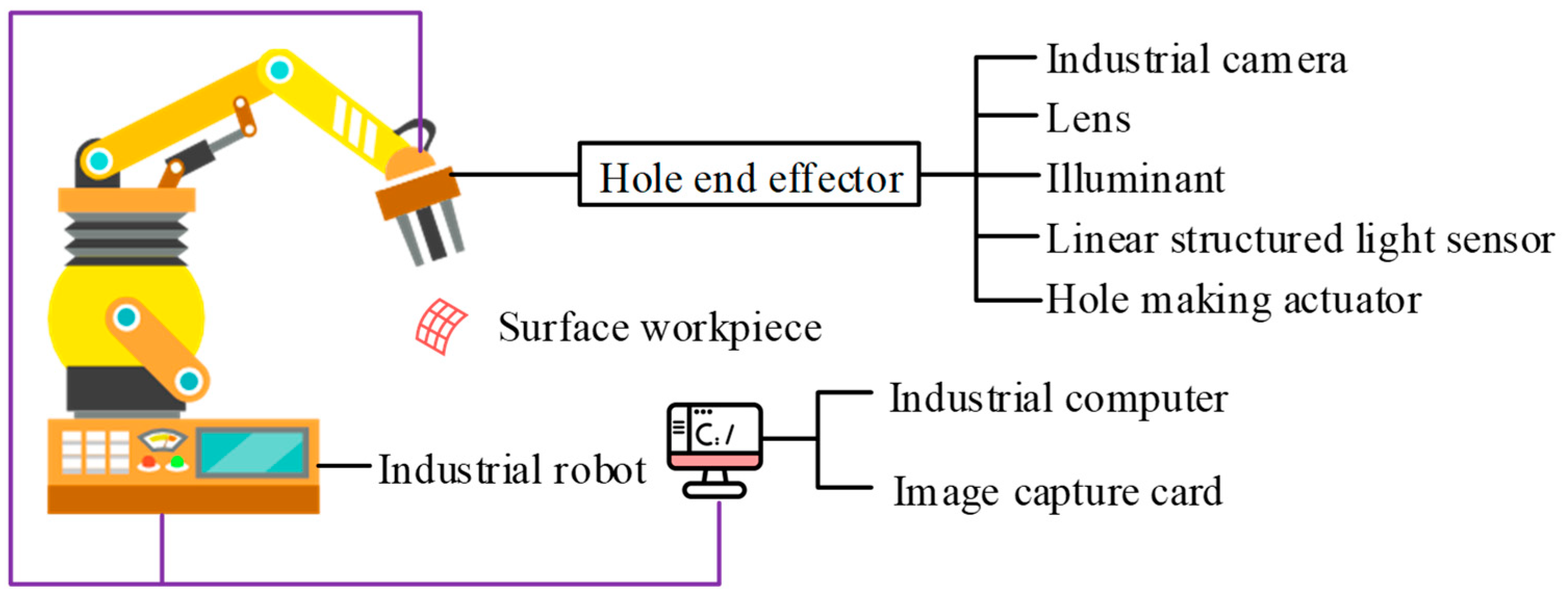
Therefore, the normal vector calculation technology developed through research is mainly aimed at aviation components with a curvature range of 0.002 mm−1 to 0.02 mm−1, corresponding to a curvature radius of 50 mm to 500 mm. To address these challenges, a design scheme for a robot hole-making system is proposed, as presented in Figure 1. The system mainly has two parts: the robot body and the vision subsystem. The robot body is equipped with specialized hole-making end effectors to ensure the stability and accuracy of hole-making operations.
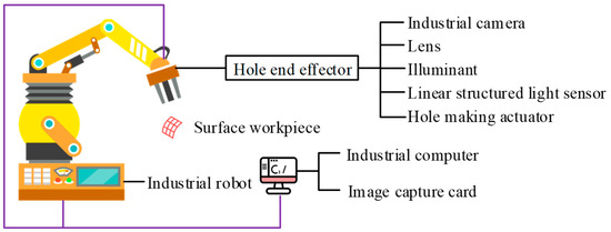
Figure 1.
Robotic hole-making system.
The robot vision subsystem, as the core of the system, integrates components such as line-structured light sensors, hole-making actuators, and industrial computers. The end effector for hole-making integrates a line-structured light sensor and an industrial camera, allowing it to obtain real-time information on the surface of the component during the hole-making process, providing accurate guidance for hole-making operations. The image acquisition card is installed inside the industrial computer, which is responsible for processing and transmitting image data, ensuring the accuracy and real-time performance of the information.
The study first establishes a unified robot system coordinate system as the basic reference framework for the entire system. Subsequently, the workpiece coordinate system and tool coordinate system are accurately calibrated. Therefore, robots can accurately control the position and posture of end effectors, ensuring the accuracy of hole-making position, direction, and depth. During the reference hole positioning stage, the robot accurately moves to the reference hole position on the workpiece. Then, high-performance industrial cameras are used to obtain clear images of the reference hole. To obtain the three-dimensional shape and position information of the workpiece, a line-structured light sensor is applied to scan the workpiece. These point cloud data are registered with the 3D CAD model point cloud to obtain the accurate pose of the workpiece in real space.
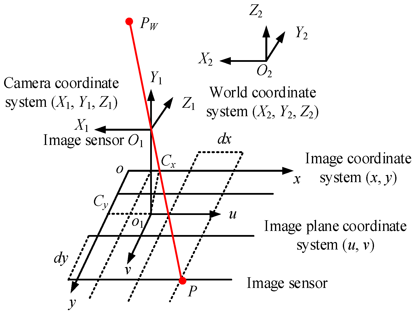
The image information obtained by industrial cameras is usually two-dimensional pixel coordinates, which cannot directly reflect the true position and posture of the workpiece in three-dimensional space [30]. In order to achieve effective conversion between spatial information and image information, the camera imaging mechanism is modeled through camera calibration. The scanning accuracy of the linear structured light sensor is ≥0.01 mm, and the resolution of the industrial camera is ≥2560 × 2048, with a frame rate of ≥138 fps, to adapt to the large size and complex curved surface characteristics of aviation components. The target measurement uncertainty of the calculation normal direction is set to ≤0.5°. It involves precise measurement and calculation of internal parameters of the camera (focal length, optical center position, lens distortion, etc.) and external parameters (the position and orientation of the camera in the world coordinate system), as well as the conversion and correlation of the camera coordinate system , image plane coordinate system , world coordinate system , and image coordinate system , as presented in Figure 2 [31]. These coordinate systems exert a meaningful role in the camera calibration process, helping to describe and calculate the relationship between image information and three-dimensional spatial information.

Figure 2.
Camera imaging model.
If the origin of the image coordinate system is in the image plane coordinate system , in the camera imaging plane, the size of a single pixel in the axis is and the size in the axis is . In this paper, the fundamental equations for 2D image processing and 2D to 3D reconstruction (Equations (1)–(3)), the principle of internal and external parameter conversion for camera calibration, and the distortion correction model (Equations (5)–(7)) all refer to the classic machine vision theory and the mature methods in the literature [32,33,34,35,36]. In view of the characteristics of large curvature components in aviation, this paper combines the above classic theories with the specific requirements of aviation manufacturing scenarios to form a hole-making accuracy control scheme suitable for large curvature surfaces.
In view of the characteristics of large curvature components in aviation, this paper combines the above classic theories with the specific requirements of aviation manufacturing scenarios to form a hole-making accuracy control scheme suitable for large single-curvature surfaces.
To accurately convert the coordinates of pixels between the image coordinate system and the image plane coordinate system, the conversion relationship between these two is represented by Equation (1) [32].
The world coordinate system is applied for precise positioning of cameras and other objects in three-dimensional space. Assuming that a point in three-dimensional space has coordinates and in coordinate systems and , the conversion relationship between the world coordinate system and the camera coordinate system is presented in Equation (2) [33].
In Equation (2), signifies the rotation matrix. signifies the translation vector, and . is the extrinsic matrix. It integrates the information of the rotation matrix and the translation vector S. Therefore, points in three-dimensional space can be accurately converted between the camera coordinate system and the world coordinate system.
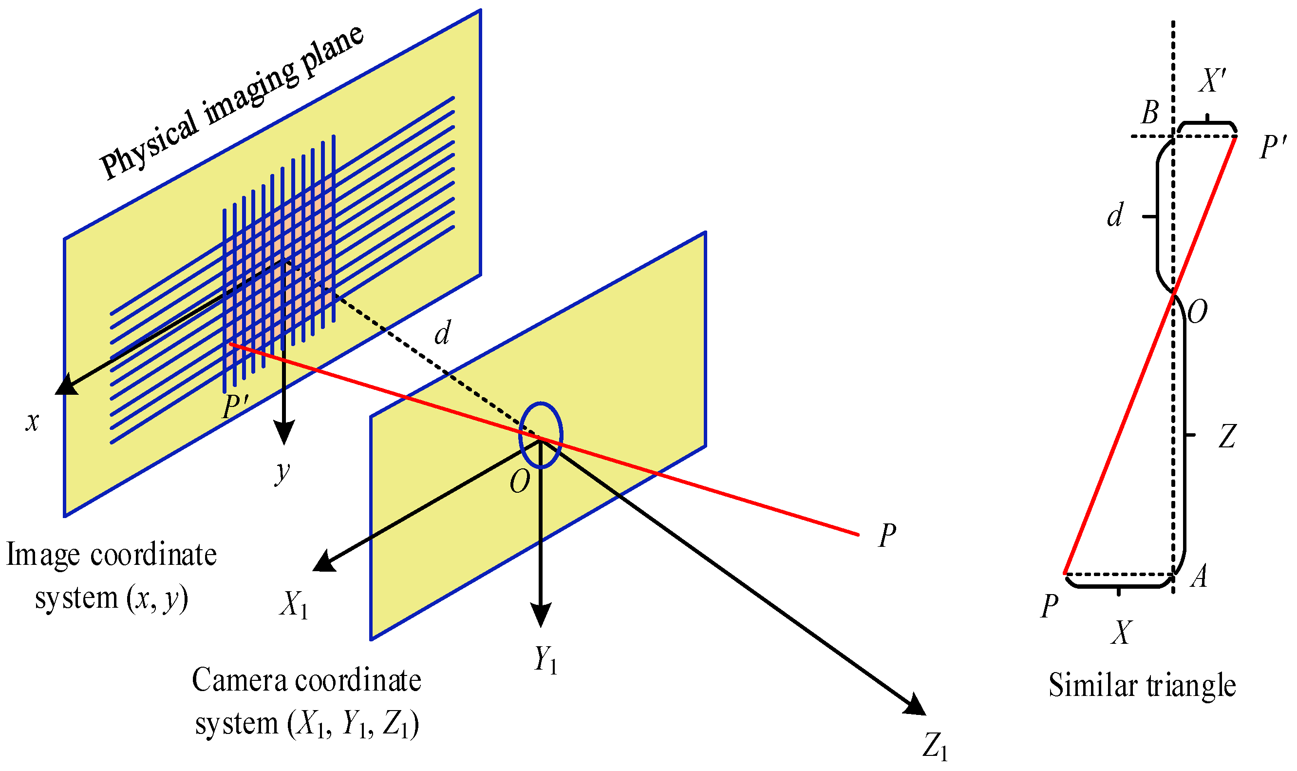
The process of mapping coordinate points in the 3D to a 2D image plane by a camera is described using a pinhole imaging model, as shown in Figure 3. Depending on the principle of similar triangles, the relationship between point in three-dimensional space and its image point on the camera imaging plane is obtained, as displayed in Equation (3) [34].

Figure 3.
Imaging model of the small hole.
In Equation (3), signifies the focal length. By applying Equations (1) and (2) to Equation (3), the transformation relationship between the image coordinate system and the world coordinate system represented is presented in Equation (4).
In Equation (4), is an orthogonal rotation matrix. Among them, , , and signify the angles at which the camera coordinate system rotates around the -axis, -axis, and -axis. signifies a translation vector. The positional relationship between the camera coordinate system and the Earth coordinate system is the extrinsic matrix of the camera. signifies the internal parameter matrix of the camera. The internal parameters of the camera are fixed after leaving the factory and will not change during use. The internal parameters are , , , and . and represent the proportional coefficients of the -axis and -axis in the image coordinate system. During the camera imaging process, distortion may occur due to factors such as the lens, so distortion correction is required to obtain the true position of objects in the image. Distortion can usually be modeled through distortion models, as shown in Equation (5) [35].
In Equation (5), signifies the coordinate of the real point on the camera imaging plane. signifies the coordinate of the image obtained in full pinhole imaging mode. and signify nonlinear distortions in the and axes. During the camera imaging process, distortion may occur due to factors such as the lens, so distortion correction is required to obtain the true position of objects in the image. Distortion usually refers to radial distortion and tangential distortion. The former is caused by the non-ideal shape of the lens. The latter is influenced by the non-parallelism between the lens and the image plane, and its functional form is displayed in Equation (6).
In Equation (6), signifies the distance from the pixel point of the image to the center point. , , and signify radial distortion parameters. and signify tangential distortion parameters. is the normalized image coordinate for ideal distortion free. The camera distortion correction model can be characterized by five distortion parameters, which can be represented by Equation (7) [36].
These parameters are obtained through the camera calibration process, which typically uses a set of known spatial coordinates of points and corresponding image coordinate points. After calibration, these distortion coefficients can be used to correct the position of points in the image, making it more accurately mapped to the spatial coordinate system.
2.2. Point Cloud Data Processing and 3D Reconstruction
After the camera calibration is completed, the point cloud data is obtained for the spatial workpiece. The study uses a line structured light sensor to collect three-dimensional point cloud data, minimizing the interference caused by external lighting and other factors on the three-dimensional point cloud collection. The line structured light sensor uses a laser beam to irradiate the surface of an object. The height information of the object surface is calculated by measuring the angle change of the laser beam reflected on the object surface, thereby obtaining the three-dimensional shape of the object, as shown in Figure 4.
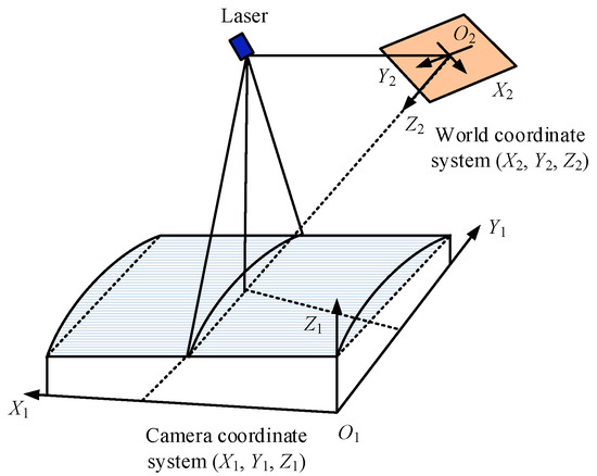
Figure 4.
Mathematical model of linear structured light sensor.
The linear structured light sensor adopted in the research is a composite sensing system that integrates laser projection and image acquisition. Its core components include a 660 nm wavelength linear laser projector and a 1.3-megapixel industrial camera, which are installed at a fixed 30° angle with the laser projector on the end effector. As shown in Figure 4, the laser projector projects linear laser fringes onto the surface of the aviation component. Due to the change in surface height, the fringes deform. The industrial camera synchronously collects the images of the deformed fringes. Based on the principle of triangulation, the three-dimensional coordinates of the surface points are calculated. Finally, the complete local point cloud data is formed by splicing the robot’s motion trajectory.
The core reason for choosing this sensing configuration lies in its active laser illumination, which can reduce the interference of external ambient light on the point cloud collection of rough and large curvature surfaces, and it is easier to obtain stable data compared with passive vision [37]. Meanwhile, this configuration achieves high-precision depth measurement through sub-pixel-level laser fringe detection, and the line scanning speed is superior to point laser scanning, which can improve data acquisition efficiency while ensuring accuracy.
In addition, its compact size can be integrated with the hole-making actuator at the end of the robot, reducing the coordinate conversion error caused by the layout of multiple sensors and simplifying the system calibration process. However, the effective scanning width of a single laser stripe is limited. For large curvature components with a diameter exceeding 100 mm, multiple scans and splicing are required, which may introduce splicing errors. When facing highly reflective surfaces such as aluminum alloys, it is easy for the stripes to be overexposed due to laser reflection, and a polarizer needs to be added. At this time, the measurement accuracy will be affected [38]. Meanwhile, during the measurement process, abnormal points that are far from the main point cloud may also occur, which seriously affects the accuracy of the point cloud [21].
However, due to limitations in the accuracy of measuring equipment, operator experience, environmental factors such as wind and vibration, and changes in the surface properties of the object being measured, point cloud data often contains noise points [39]. The complex working environment, measurement errors, equipment accuracy, and other factors involved in the assembly and hole-making of aviation structural components can also lead to abnormal points far from the main point cloud, thereby seriously affecting the point cloud accuracy.
A data processing approach on the basis of statistical filters is designed to handle the outlier removal in point cloud data. This method assumes that the distance among points in a point cloud follows a Gaussian distribution. First, the nearest neighbor point is found on the point cloud surface, and then the nearest neighbor sequence is statistically analyzed. The quantity of points in the point cloud is . -nearest neighbor search is performed on point and the average distance between and its neighboring points is calculated. The average value and standard deviation of the distance set are calculated as shown in Equation (8).
According to the Gaussian distribution, Equation (9) is used to calculate the distance threshold.
In Equation (9), is a multiple of the standard deviation. The threshold is determined by the . In practical applications, it should be appropriately selected based on the distribution of discrete points in the point cloud. By determining the relationship between the mean and threshold of each point in its neighbors, if the mean deviates from this interval, it will be removed. Point cloud reconstruction on the basis of point cloud data can restore the surface morphology of the measured object, facilitating subsequent detection and visualization. The study first fits a certain part of the fitting domain. The fitting function is obtained, as displayed in Equation (10).
In Equation (10), signifies the coefficient to be calculated and is a function of the coordinate . signifies the quantity of items in the basis function. is a -class complete polynomial, also known as a basis function. The weight function is the core of the sliding least squares algorithm, which means that within the influence range of (also known as the support domain of the weight function), its weight functions are all greater than 0. If it exceeds its scope of influence, it is 0. Usually, a circular area is selected as the support area, and its radius is represented by . According to the compactness of the weight function, it can be known that only the points on this circular region have an impact on the . The weighting function has a non-negative monotonic decay and a high degree of smoothness, as shown in Equation (11).
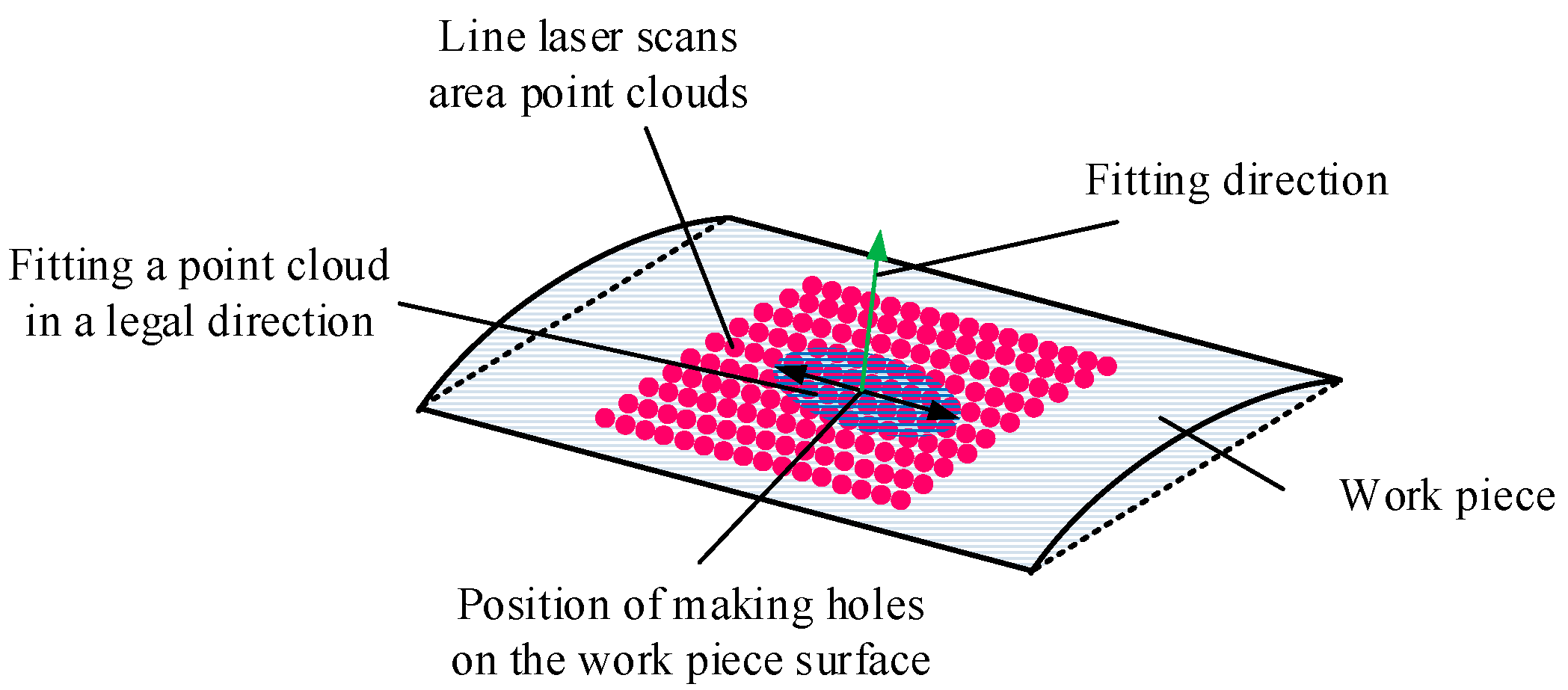
In Equation (11), . signifies the of the support region for the weight function of the -th node. is the influencing factor, usually between 1.25 and 2.5. Although there have been studies using linear laser line scanning methods to obtain three-dimensional point clouds of large and complex curved parts, further research is necessary on how to obtain high-precision surface normals. Figure 5 shows the proposed normal calculation model for large curvature surfaces. Firstly, a hole shape on the surface of a large curvature part is selected as the center of the circle. Based on this center, a circular area with a diameter of is established and point cloud data within this area is collected. The collected point cloud data is subjected to plane fitting using PCA, and the normals on the surface are replaced with the normals processed into hole points [40]. The selected point cloud is evenly distributed in the selected circular domain. When selecting the appropriate diameter value, its region is very close to the plane. Using the plane fitting method to calculate the normal vector can achieve good accuracy.

Figure 5.
Normal calculation method for large curvature surface.
Normal calculation is carried out before drilling. Firstly, during the clamping stage, three reference holes are identified. The coordinates are collected by an industrial camera to complete the registration of the point cloud with the CAD model and eliminate clamping offset. Select a local point cloud around the theoretical hole-making point, calculate the actual normal using the PCA algorithm, and at the same time ensure that the positioning error matches the normal error through local point cloud constraints. Pre-drill and verify the key parts. When the deviation exceeds the limit, recalibrate to ensure that the theoretical normal is accurately applied to the actual hole-making points.
The algorithm for normal estimation has the following components:
- Inputs: Raw point cloud data from the structured-light sensor, surface curvature radius, and predefined point-cloud selection diameter.
- Outputs: The estimated surface normal vector at the selected point, the calculated angular deviation from the theoretical normal, and the filtered point cloud after denoising.
- Decision Criteria: The point cloud neighborhood is adaptively expanded until the true proportion PPP of valid points exceeds the confidence threshold (60%), ensuring that PCA fitting error remains ≤0.2°.
The surface fitting calculation method adopts PCA, which utilizes multidimensional orthogonal linear transformation to make it linearly correlated in various dimensions. It can effectively extract important features of data, which is usually used for dimensionality reduction in high-dimensional data. Using pieces of raw point cloud data as samples, where signifies one of the data, a set of matrices is obtained by fitting it. The covariance matrix is obtained using Equation (12):
The covariance matrix and its corresponding eigenvalues are obtained. signifies a diagonal matrix. signifies a three-level feature matrix, which has three sets of eigenvectors of . The two eigenvectors in are used as the base vectors on the point cloud plane according to their respective eigenvalues, and the eigenvector corresponding to the smallest eigenvalue is the normal vector of the surface.
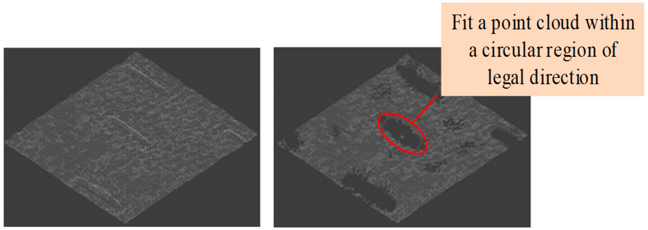
To ensure the accuracy of normal fitting, the appropriate point cloud data is selected to perform normal fitting on the large curvature surface during the normal solution process [41]. However, due to the many irregular protrusions on the surface of the tested object, point cloud holes may appear after removing the protrusion characteristic point cloud. From Figure 6, when selecting a small radius, the proportion of voids in this range is too large, which will affect the accuracy of forward calculation. However, the larger the radius, the smaller the impact of the hole on the model. Using other point cloud fitting methods within this range can also ensure the accuracy of the model.

Figure 6.
Cloud holes at points.
To address the impact of cavities on the accuracy of normal fitting, a method based on the proportion of point clouds in the selected circular domain is proposed. The true proportion of the point cloud is defined in Equation (13).
In Equation (13), is the density of the point cloud before eliminating the protrusion characteristic. is the area of the circular region. is the current number of point clouds in the selected range. When , the diameter of the annular region should be appropriately increased. The reasons for setting the confidence threshold to 60% are as follows:
- By verifying the surface point cloud data of aviation components with different curvatures, it was found that when , the local point cloud caused the PCA plane fitting error to exceed the target measurement uncertainty due to the excessively high proportion of voids.
- When , the uniformity of point cloud distribution can meet the requirements of normal fitting accuracy.
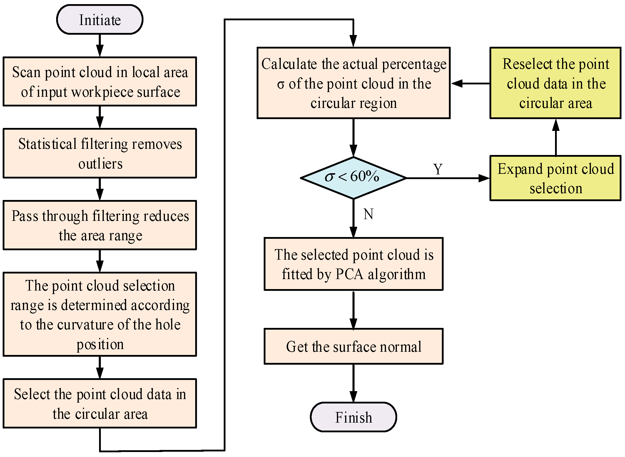
Considering the large curvature and numerous irregular protrusions on the surface of the object being measured, a detailed calculation process for this method is presented in Figure 7.
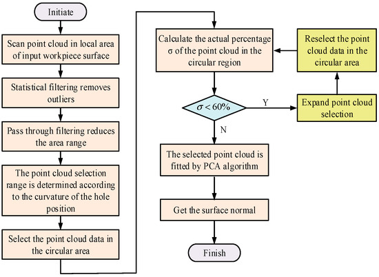
Figure 7.
Normal solution flow chart.
Firstly, the scanning point cloud of the local area on the surface of the workpiece is input, and the input point cloud data is denoised to eliminate measurement errors and noise points caused by the external environment. Then, the curvature changes on the surface of the workpiece are analyzed, especially the curvature of the hole-making position. Based on the curvature size, a suitable circular area diameter is determined, which should be large enough to contain necessary surface information but not too large to contain too much irrelevant data. Based on the diameter and position of the circular area determined in the previous step, the point cloud data located within the circular area is selected from the preprocessed point cloud data. If , the selected range diameter of the point cloud is expanded. Finally, the PCA algorithm is used to perform plane fitting on the selected point cloud to achieve the normal direction of the curved surface.
The robot automatic hole-making system constructed in the research simultaneously processes positional errors and normal errors to ensure the integrity of hole-making accuracy. For normal errors, the system adopts an offline verification and correction mechanism. The specific process is as follows: Firstly, a comprehensive scan of the workpiece surface is conducted through a line-structured light sensor to complete surface digitization and obtain high-precision point cloud data.
Subsequently, based on the preprocessed point cloud data, the normal vector of the position of the hole to be fabricated is calculated using the PCA algorithm and compared with the theoretical normal. If the normal error exceeds the allowable range (set as 0.5° in this study), iterative compensation is carried out by adjusting the local point cloud extraction range (dynamically optimizing the diameter of the circular area according to the process in Figure 7) and the PCA parameters, and the normal vector is recalculated until the error meets the requirements. Ultimately, the corrected normal parameters are input into the robot control system to guide the hole-making operation.
3. Performance Verification of Robot Automatic Hole-Making
The study compares the denoising effect of point cloud preprocessing algorithms before and after optimization. By measuring large curvature surfaces in practice, the difference between the calculated normal and theoretical values is compared to assess the accuracy of the calculation method. As for the development environment and tools, Visual Studio 2019 and Qt5.14.2 are chosen as the development platforms for the normal measurement software. By comparing experimental data with theoretical expectations, the accuracy and stability of the measurement system are validated.
3.1. Preprocessing Effect of Point Cloud Data
Considering the strict requirements for clamping force during robot hole machining, the R-2000iC/165F industrial robot from FANUC and the SP-5000C-CPX4 high-speed camera from JAI are selected. Among them, FANUC robots have excellent load capacity and high-precision positioning performance. High-speed cameras from JAI have high definition and fast image capture capabilities, providing high-quality image data for measurement systems. Table 1 presents relevant parameters.

Table 1.
Parameter details.
Composite flat plates and aluminum alloy arc parts are widely used in industrial manufacturing, which can validate their universality and applicability. The study aims to quickly obtain 3D information of the surfaces of composite flat plates and aluminum alloy circular arc parts through line laser scanning. To ensure the stability and accuracy of the scanning, the line scanning speed is set to 1 mm/s, and the scanning-collected point cloud data is preprocessed, as presented in Figure 8. The preprocessed point cloud data was more streamlined, with effective removal of noise and redundancy. At the same time, the accuracy and reliability of the data were greatly improved.
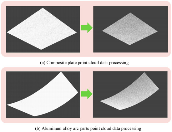
Figure 8.
Preprocessing effect of point cloud data for (a) Composite plate point and (b) Aluminum alloy.
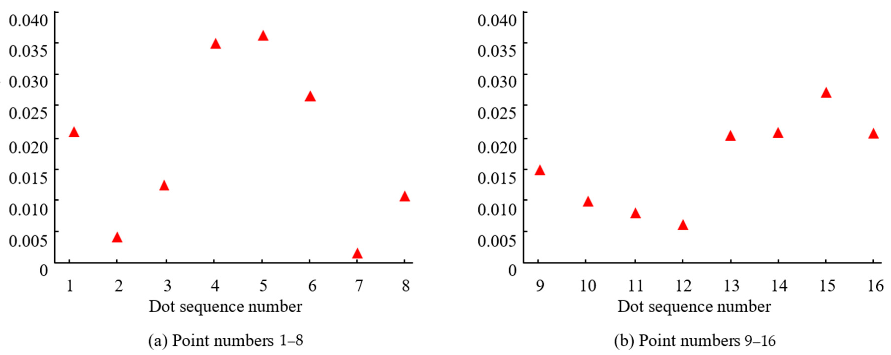
Due to the fact that not all calibration values can meet the accuracy requirements, it is necessary to verify the calibration results to ensure that the error is small and the accuracy satisfies the requirements. According to the calibration data, the position and orientation parameters, sensor measurement values, and corresponding standard surfaces of each laser displacement sensor are calibrated. The calibration deviation values are shown in Figure 9. From the figure, the calibration deviation of 16 points corresponding to 8 sets of data remained within 0.04 mm, which met the accuracy requirements.
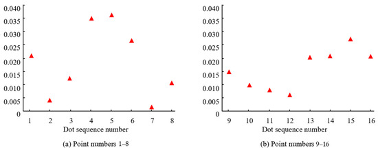
Figure 9.
Schematic diagram of calibration deviation values for (a) Point number 1–8 and (b) Point numbers 9–16.
The influence of part stiffness on hole-making accuracy is controlled in the proposed system through a combination of adaptive support fixtures and real-time force monitoring. For thin-walled parts that are prone to deformation, vacuum suction cups and rigid fixtures are employed to reduce local deflection caused by drilling forces. The axial drilling force is continuously monitored via force sensors, and the feed rate is adaptively adjusted whenever the force exceeds a defined threshold. These measures ensure that the deformation of thin-walled parts remains within ≤0.05 mm during drilling.
3.2. Error Analysis
Super depth microscope is used to observe hole-making workpieces. Through the high-resolution imaging system of the microscope, the actual hole position is accurately measured. In order to quantify errors and provide a unified reference benchmark for error analysis, a two-dimensional coordinate system is defined in the study. Among them, the Y signifies the direction from the center of the hole to the right edge of the workpiece, and the X signifies the direction from the center of the hole to the bottom edge of the workpiece.
The error data of the drilled workpiece is displayed in Table 2. For position errors, the system establishes an accurate coordinate transformation relationship through camera calibration and compares the actual hole position with the theoretical hole position by combining point cloud registration technology, as shown in Table 2. Among them, x and y, respectively, represent the deviation values of the actual coordinates and theoretical coordinates of the hole-making position in the two-dimensional coordinate system. This coordinate system takes the theoretical center of the hole-making position as the origin, with the X-axis representing the direction from the center of the hole to the bottom edge of the workpiece and the Y-axis representing the direction from the center of the hole to the right edge of the workpiece.

Table 2.
Machining error of hole-making.
The maximum error in the X direction of the machined hole was 0.25 mm, the maximum error in the Y-axis was 0.20 mm, and the maximum root mean square error was 0.252 mm. Across six measurement points, the mean position error was 0.11 ± 0.14 mm (X-axis) and 0.07 ± 0.11 mm (Y-axis), based on n = 6 trials. The small mean values relative to the process tolerance (±0.3 mm) and low standard deviations indicate high repeatability and minimal systematic bias in hole placement. The error data shows that the error of all measurement points is less than 0.3 mm, which satisfies the process requirements and verifies its reliability. It also provides strong support for subsequent process optimization and quality control.
The equipment used for measurement is a super-depth-of-field microscope (Keyence VHX-7000 (manufactured by Keyence Corporation, Osaka, Japan)), which can precisely identify the edge coordinates of the hole through a high-resolution imaging system to calculate the deviation. The errors in the table are all individual measurement errors, that is, the differences between the actual center coordinates and the theoretical center coordinates of each hole.
The root mean square error is the root mean square value of the position errors of the six measurement holes, and the measurement sequence is the single measurement result of the six machined holes. As can be seen from the table, the maximum error of the X-axis is −0.25 mm, the maximum error of the Y-axis is −0.20 mm, and the maximum root mean square error is 0.252 mm, which conforms to the actual precision range of robot processing of large aviation parts and is all less than the 0.3 mm error threshold allowed by the process.
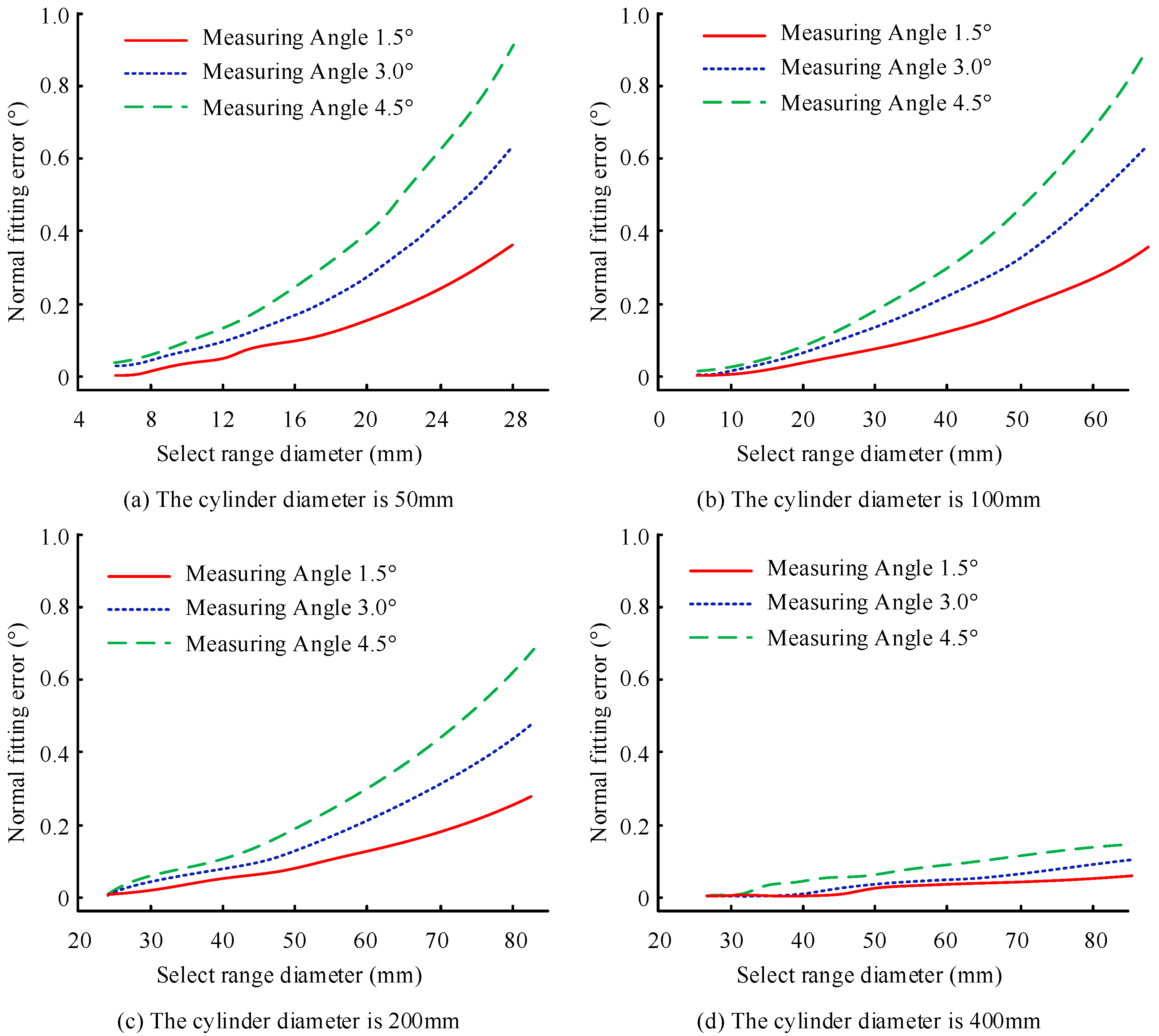
Due to the significant curvature of the fuselage wall panels in aerospace components in one direction, while they are relatively straight in another direction, they can be approximated as a cylindrical surface with a fixed radius in practical analysis and processing. This approximation helps simplify the calculation and analysis process, as the geometric properties of cylindrical surfaces are relatively simple and easy to handle. In response to the curvature characteristics of aerospace components, the study first selects several representative typical values and then generates corresponding cylindrical point cloud data. The law of error variation with the selection range of point cloud is further analyzed, as displayed in Figure 10.
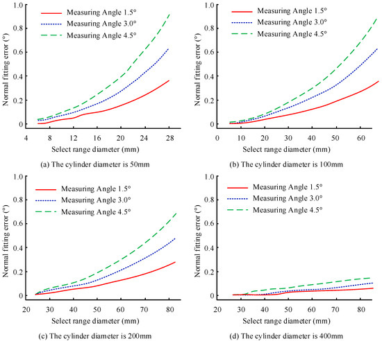
Figure 10.
Changes in point cloud range, angle measurement methods, and fitting errors for cylinder diameters of (a) 50 mm (b) 100 mm (c) 200 mm and (d) 400 mm.
In Figure 10b, when the diameter of the cylinder was 100 mm and the selection range of the point cloud was 20 mm, the measurement error of 4.5° was 0.019° larger than that of 1.5°. When the selection range of the point cloud was 40 mm, the measurement error of 4.5° was 0.127° larger than that of 2°. From Figure 10a,c,d, with fixed curvature and measurement angle, the larger the selection range of the point cloud, the greater the normal fitting error, and it shows a nonlinear growth trend. When the point cloud range is small, the curvature has a relatively small impact on the normal fitting error due to the relatively simple distribution of point cloud data. Once the selection range of point clouds increases to a certain extent, the influence of curvature becomes particularly significant, leading to a significant increase in the deviation between the fitted normal and the actual normal.
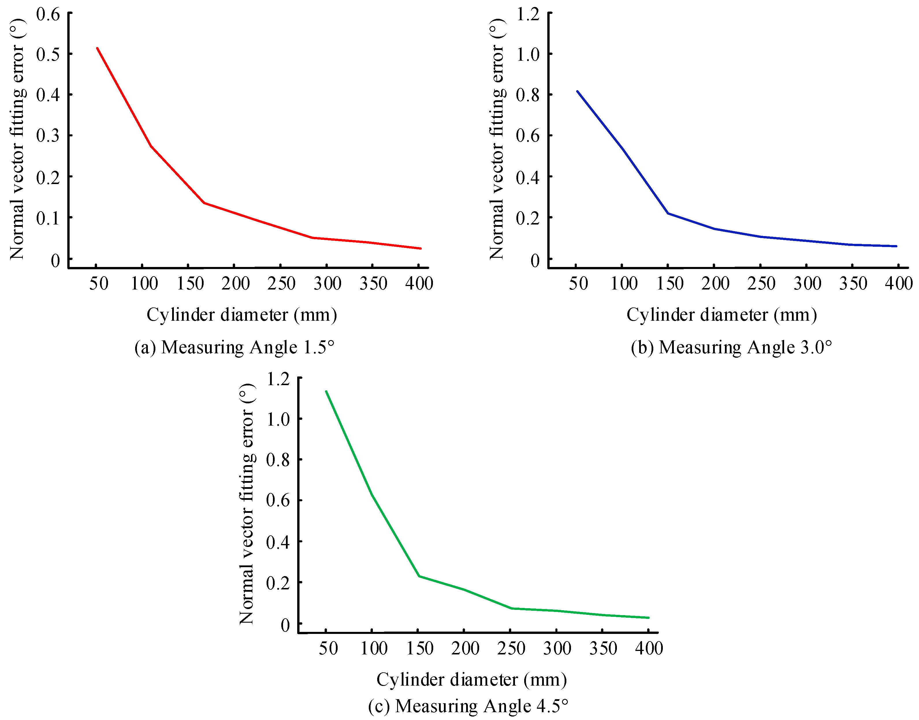
The study investigates the relationship between normal fitting error and curvature while maintaining a constant measurement angle and a fixed range of point cloud selection. Taking the point cloud range diameter of 30 mm as an example, the corresponding normal fitting error data is shown in Figure 11. From Figure 11, there was an inverse relationship between curvature and normal fitting error. This is because when the curvature is small, the area where the point cloud data is located is closer to the plane, which makes the process of fitting the normal direction simpler and more accurate.
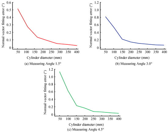
Figure 11.
Influence of curvature on normal fitting error for Measuring angles of (a) 1.5 °, (b) 3.0°, and (c) 4.5°.
For a cylinder with a diameter of 400 mm, point cloud selection within 100 mm had high normal fitting accuracy. However, when selecting the range of point cloud data, the measurement line width limitation of the line laser sensor and the impact of point cloud data processing time should be considered. If the selected range is too large, it may cause the sensor to be unable to measure accurately or the processing time to be too long, affecting work efficiency.
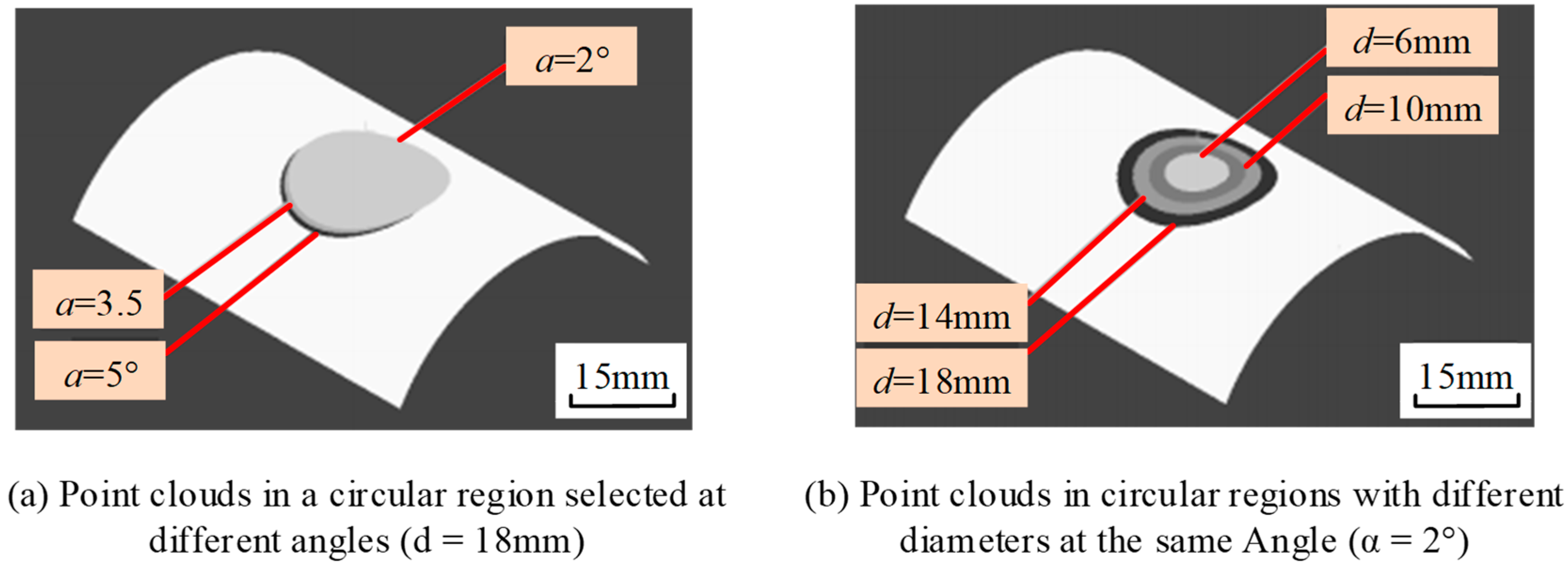
Aluminum alloy is selected as the experimental material for the study, and a cylindrical test specimen with a diameter of 50 mm is prepared through precision machining. To achieve accurate data on the surface of the test piece, a line laser sensor is used as the data acquisition tool for validation through point cloud data from four different diameter regions. The selection of point clouds is shown in Figure 12. This multi-angle and multi-scale verification method can comprehensively assess the performance and ensure accurate results under various conditions.
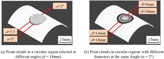
Figure 12.
Point cloud selection in the circular area for (a) different angles and (b) same angle.
The proposed algorithm is used to process and calculate the normal fitting error, as presented in Table 3. Whether it was measured data or simulated data, the normal fitting error showed a similar trend with the change in point cloud selection range diameter, demonstrating a high degree of accuracy in capturing and predicting the normal fitting error with the change in point cloud range. For each measuring angle, four point cloud selection ranges were tested (n = 4 per angle). The mean ± standard deviation of normal fitting errors were 0.151 ± 0.054° (1.5°), 0.215 ± 0.096° (3.0°), and 0.269 ± 0.118° (4.5°). This low variability across different selection ranges at the same angle indicates consistent estimation performance and supports the method’s repeatability.

Table 3.
Normal fitting errors.
The normal fitting error in actual measurement processes is due to various factors, including the complexity of the measurement environment, differences in the test specimens themselves, limitations of measurement equipment, issues with data processing and algorithm implementation, and simplification of simulation models. However, by carefully selecting and processing point cloud data, this error can be effectively controlled to ensure its accuracy meets the strict requirements of the aerospace manufacturing industry for hole verticality. This discovery not only validates the feasibility and effectiveness of the proposed algorithm in practical applications but also provides a new and reliable method for controlling normal fitting errors in the aerospace manufacturing industry.
The proposed algorithm is applied in two stages: (1) pre-drilling adjustment, where the normal direction of the drill is corrected by comparing the calculated surface normal with the theoretical CAD normal, and the robot end effector is reoriented to minimize angular deviation; and (2) post-drilling quality verification, where the point cloud around the drilled hole is re-scanned to measure the hole diameter, verticality, and deviation. If the dimensional tolerance exceeds process requirements, a secondary corrective drilling operation is triggered.
A simulated baseline was generated using a fixed point cloud range diameter of 30 mm, representing a standard fixed-parameter alignment approach. The simulation results for measuring angles of 1.5°, 3.0°, and 4.5° produced normal fitting errors of 0.52°, 0.78°, and 1.12°, respectively, as shown in Table 4 and illustrated in Figure 11. By contrast, the adaptive PCA method reduced these errors to 0.079°, 0.111°, and 0.147°, corresponding to improvements of 84.8%, 85.8%, and 86.9%. This simulation demonstrates that dynamic neighborhood selection can significantly outperform fixed-parameter methods in scenarios with varying curvature.

Table 4.
Simulated baseline fixed-parameter method (30 mm range) vs. adaptive PCA.
3.3. Influence of Surface Roughness and Curvature on Normal Estimation
To further validate the proposed normal calculation algorithm, the influence of surface roughness and curvature radius on normal fitting accuracy was analyzed through comparative experiments. Four typical surface roughness levels and four curvature radii were selected for the experiment. The normal fitting errors were tested within the range of point cloud extraction (diameter 30 mm), and the results are shown in Table 5.

Table 5.
Comparative analysis of the influence of surface roughness and radius of curvature on normal estimation.
The industrial camera adopted in this study can distinguish the peak and valley characteristics corresponding to Ra6.3 roughness. Through the spectral analysis of the point cloud data on the Ra6.3 surface, the point cloud collected by the camera retains over 90% of the roughness features at the scale of 0.01–0.1 mm. It can be seen from the table that under the same radius of curvature, the normal error increases linearly with the increase in roughness (when Ra1.6 to Ra6.3, the error increase is approximately 40–78%). Under the same roughness, the normal error increases nonlinearly as the radius of curvature decreases (curvature increases) (the error at a radius of 50 mm is approximately 3 to 4 times that at 400 mm).
It can be seen from this that the influence of the radius of curvature on the normal error is significantly greater than that on the surface roughness, and it is a factor that needs to be controlled first. Moreover, a rough surface can cause high-frequency fluctuations in local point clouds, introducing deviations into the PCA plane fitting. From the above experiments, it can be known that when the roughness is ≤Ra4.8, the point cloud after preprocessing can meet the requirement of a normal error of ≤0.2°. When the roughness is greater than Ra4.8, the error needs to be compensated by optimizing the neighborhood parameters or increasing the point cloud extraction range to ensure that the target measurement uncertainty (≤0.5°) is met.
The results demonstrate that while the proposed normal estimation algorithm achieves high accuracy (≤0.2°), the overall hole quality is still influenced by drilling forces and the rigidity of thin-walled components. High cutting forces can introduce minor deviations due to elastic deflection, particularly when the local stiffness is insufficient. Our approach mitigates these effects through the use of adaptive vacuum fixtures and real-time force monitoring, but further integration of force modeling and tool wear prediction—as suggested by [4,16]—could improve stability under extreme drilling conditions.
This study prioritizes the selection of aluminum alloy as the specimen for the following reasons: (1) Aluminum alloy is the core material of aviation structures, accounting for 60% to 80% of the fuselage weight, and its processing characteristics have a significant impact on the hole-making accuracy; (2) Compared with carbon fiber composite materials, the surface properties of aluminum alloys are more stable, and there is no uneven reflection caused by the fiber direction. The basic validity of the normal fitting algorithm can be proved a priori.
4. Conclusions
In response to the measurement challenges of high curvature and surface roughness in aerospace components, a set of normal calculation methods suitable for high curvature aerospace components was designed by combining point cloud data preprocessing and 3D reconstruction results. The experimental results showed that after the preprocessing steps, the point cloud data was significantly simplified and the data quality was greatly improved. The preprocessed point cloud data was more streamlined, with effective removal of noise and redundancy.
The maximum error in the X-axis of the machining hole was 0.191 mm, the maximum error in the Y-axis was 0.174 mm, and the maximum root mean square error was 0.197 mm. The error data showed that the error of all measurement points was less than 0.3 mm, which met the process requirements. When the cylindrical surface was 100 mm and the selection range of the point cloud was 10 mm, the measurement error of 4.5° was 0.020° larger than that of 1.5°. When the selection range of the point cloud was 30 mm, the error increased to 0.127 mm.
For cylindrical surfaces with a diameter not exceeding 400 mm, as long as the selected point cloud range did not exceed 100 mm, the normal error was controlled within a very small range. The above results indicate that by reasonably selecting the range of point cloud data and improving the accuracy of normal fitting, the quality and reliability of aerospace components can be improved, and rework and scrap caused by non-compliance with verticality requirements can be reduced, thereby lowering production costs. This study mainly focuses on aerospace components with significant large curvature in a single direction. By clarifying the variation law of normal fitting error under different curvature conditions, the accuracy of the robot hole-making system has been improved. However, for complex components that exhibit significant curvature in multiple directions, the precise calculation of surface normal is a challenging problem. In the future, higher-order surface models such as quadratic and cubic surfaces can be considered to replace simple plane fitting in order to better adapt to the surface shapes of complex components.
Furthermore, the study verified the effectiveness of the composite 3D sensing system, which integrates structured-light projection and a linear laser with an industrial camera. By reconstructing high-resolution point clouds through triangulation, the proposed PCA-based adaptive normal estimation algorithm achieved robust performance, maintaining normal accuracy ≤ 0.2° even under varying surface roughness and curvature conditions. The current system performance was validated under controlled laboratory conditions; in field environments, factors such as high surface reflectivity, excessive roughness (Ra > 6.3), and vibration may impact measurement accuracy. While a polarizing filter mitigates laser overexposure on reflective alloys, it can slightly reduce precision. Additionally, the structured-light sensor’s effective scanning width limits point cloud coverage for components exceeding 100 mm curvature diameter, requiring multiple passes and increasing processing time.
Although the algorithm effectively compensates for normal errors, the overall hole quality remains influenced by drilling forces and thin-wall rigidity. The use of adaptive fixtures and real-time force monitoring in this study successfully limited deformation to ≤0.05 mm, but future work will integrate cutting force modeling and tool wear prediction to further enhance stability and hole precision.
Author Contributions
Methodology, validation, investigation, resources, writing—original draft, H.Y., R.G., B.D., Y.B., and Y.Q.; writing—review and editing, R.G. and B.D.; supervision, Y.B. All authors have read and agreed to the published version of the manuscript.
Funding
This study did not receive any funding.
Informed Consent Statement
Not applicable.
Data Availability Statement
Data will be made available on request.
Conflicts of Interest
The authors declare no conflict of interest.
Abbreviations
| AI | Artificial Intelligence |
| CAD | Computer-Aided Design |
| CNC | Computer Numerical Control |
| CNN | Convolutional Neural Network |
| FPS | Frames per Second |
| PCA | Principal Component Analysis |
| RMS | Root Mean Square |
| SL | Structured Light |
| 3D | Three-Dimensional |
| 2D | Two-Dimensional |
| Ra | Roughness Average |
| RGB | Red–Green–Blue |
| SLAM | Simultaneous Localization and Mapping |
| CCD | Charge-Coupled Device |
References
- Adel, A. The Convergence of Intelligent Tutoring, Robotics, and IoT in Smart Education for the Transition from Industry 4.0 to 5.0. Smart Cities 2024, 7, 325–369. [Google Scholar] [CrossRef]
- Zhao, D.; Guo, W. Shape and Performance Controlled Advanced Design for Additive Manufacturing: A Review of Slicing and Path Planning. J. Manuf. Sci. Eng. Trans. ASME 2020, 142, 10801. [Google Scholar] [CrossRef]
- Yin, Z.; Liu, Q.; Sun, P.; Ding, J. Kinematic Analysis and Parameter Measurement for Multi-Axis Laser Engraving Machine Tools. Machines 2021, 9, 237. [Google Scholar] [CrossRef]
- Ishfaq, K.; Asad, M.; Mahmood, M.A.; Abdullah, M.; Pruncu, C. Opportunities and Challenges in Additive Manufacturing Used in Space Sector: A Comprehensive Review. Rapid Prototyp. J. 2022, 28, 2027–2042. [Google Scholar] [CrossRef]
- Klocke, F.; Soo, S.L.; Karpuschewski, B.; Webster, J.A.; Novovic, D.; Elfizy, A.; Axinte, D.A.; Tönissen, S. Abrasive Machining of Advanced Aerospace Alloys and Composites. CIRP Ann. Manuf. Technol. 2015, 64, 581–604. [Google Scholar] [CrossRef]
- Rambabu, P.; Prasad, N.E.; Kutumbarao, V.V. Aerospace Materials and Material Technologies; Springer: Berlin/Heidelberg, Germany, 2017; Volume 2, ISBN 978-981-10-2142-8. [Google Scholar]
- Li, J.; Zhou, G.; Zhang, C. A Twin Data and Knowledge-Driven Intelligent Process Planning Framework of Aviation Parts. Int. J. Prod. Res. 2022, 60, 5217–5234. [Google Scholar] [CrossRef]
- Bhundiya, H.G.; Royer, F.; Cordero, Z. Engineering Framework for Assessing Materials and Processes for In-Space Manufacturing. J. Mater. Eng. Perform. 2022, 31, 6045–6059. [Google Scholar] [CrossRef]
- Sarh, B.; Buttrick, J.; Munk, C.; Bossi, R. Aircraft Manufacturing and Assembly. In Springer Handbook of Automation; Springer: Berlin/Heidelberg, Germany, 2009; pp. 893–910. [Google Scholar] [CrossRef]
- Gohardani, A.S.; Doulgeris, G.; Singh, R. Challenges of Future Aircraft Propulsion: A Review of Distributed Propulsion Technology and Its Potential Application for the All-Electric Commercial Aircraft. Prog. Aerosp. Sci. 2011, 47, 369–391. [Google Scholar] [CrossRef]
- Szarski, M.; Chauhan, S. An Unsupervised Defect Detection Model for a Dry Carbon Fiber Textile. J. Intell. Manuf. 2022, 33, 2075–2092. [Google Scholar] [CrossRef]
- Dai, J.; Shen, J.; Tian, W.; Li, P.; Liu, H.; Cui, X. Benchmark Feature Detection Method for Mobile Robot Automatic Drilling System Integrated with Deep Learning. Machines 2025, 13, 154. [Google Scholar] [CrossRef]
- Ding, Z.; Li, R. Point Cloud Reduction Method Based on Curvature Grading and Voxel Filtering. J. Electr. Syst. 2024, 20, 318–326. [Google Scholar] [CrossRef]
- Szarski, M.; Chauhan, S. Instant Flow Distribution Network Optimization in Liquid Composite Molding Using Deep Reinforcement Learning. J. Intell. Manuf. 2023, 34, 197–218. [Google Scholar] [CrossRef]
- Ruiz, L.; Díaz, S.; González, J.M.; Cavas, F. Improving the Competitiveness of Aircraft Manufacturing Automated Processes by a Deep Neural Network. Integr. Comput. Aided. Eng. 2023, 30, 341–352. [Google Scholar] [CrossRef]
- Herzog, T.; Brandt, M.; Trinchi, A.; Sola, A.; Molotnikov, A. Process Monitoring and Machine Learning for Defect Detection in Laser-Based Metal Additive Manufacturing. J. Intell. Manuf. 2024, 35, 1407–1437. [Google Scholar] [CrossRef]
- Zhou, G.; Zhou, K.; Zhang, J.; Yuan, M.; Wang, X.; Feng, P.; Zhang, M.; Feng, F. Digital Modeling-Driven Chatter Suppression for Thin-Walled Part Manufacturing. J. Intell. Manuf. 2024, 35, 289–305. [Google Scholar] [CrossRef]
- Zhu, K.; Fuh, J.Y.H.; Lin, X. Metal-Based Additive Manufacturing Condition Monitoring: A Review on Machine Learning Based Approaches. IEEE/ASME Trans. Mechatron. 2022, 27, 2495–2510. [Google Scholar] [CrossRef]
- Lin, J.; Zheng, B.; Chen, Z. Application of Data Visualization Interaction Technology in Aerospace Data Processing. Scalable Comput. 2023, 24, 641–650. [Google Scholar] [CrossRef]
- Fan, W.; Fu, Q.; Cao, Y.; Zheng, L.; Zhang, X.; Zhang, J. Binocular Vision and Priori Data Based Intelligent Pose Measurement Method of Large Aerospace Cylindrical Components. J. Intell. Manuf. 2024, 35, 2137–2159. [Google Scholar] [CrossRef]
- Simonov, E.N.; Vinogradov, K.M.; Gorozhankin, A.N.; Anikin, A.S.; Khryukin, D.Y. Development and Modeling of a 3D Image Reconstruction Algorithm for Cone-Beam X-Ray Computed Tomography for Non-Destructive Testing in Additive Manufacturing. Russ. Eng. Res. 2024, 44, 563–568. [Google Scholar] [CrossRef]
- Takahashi, H.; Oki, J.; Hirotani, T.; Taguchi, H. Tomographic Reconstruction of Hypersonic Winged Aircraft Model Flowfields in Large-Scale Hypersonic Wind Tunnel Experiment. In Proceedings of the 25th AIAA International Space Planes and Hypersonic Systems and Technologies Conference, Bengaluru, India, 28 May–1 June 2023; Volume 62, pp. 869–881. [Google Scholar] [CrossRef]
- Zhao, E.; Zhang, Y.; Gao, J. Monocular Depth Estimation of Noncooperative Spacecraft Based on Deep Learning. J. Aerosp. Inf. Syst. 2023, 20, 334–342. [Google Scholar] [CrossRef]
- Olubodun, P.A.; Fischer, J.D.; Bristow, D.A. Iterative Correction of Robotic Grinding Using Spatial Feedback for Precision Applications. Manuf. Lett. 2024, 41, 264–269. [Google Scholar] [CrossRef]
- Miao, Y.; Wang, Z.; Zhang, X.; Xu, S.; Cai, Z.; Peng, X.; Liu, X. Large Depth-of-Field 3D Measurement with Multi-View Fusion in MEMS-Based Structured Light Field. Opt. Express 2025, 33, 28122–28140. [Google Scholar] [CrossRef]
- Alam, M.A.; Ya, H.H.; Sapuan, S.M.; Mamat, O.; Parveez, B.; Yusuf, M.; Masood, F.; Ilyas, R.A. Recent Advancements in Advanced Composites for Aerospace Applications: A Review. In Advanced Composites in Aerospace Engineering Applications; Springer: Cham, Switzerland, 2022; pp. 319–339. [Google Scholar] [CrossRef]
- HB 7759-2004; Coding for Aircraft Product Structure. China Machinery Industry Federation: Beijing, China, 2004.
- SAE AS 9100D; Quality Management Systems—Requirements for Aviation, Space, and Defense Organizations AS9100D. SAE International: Warwick, PA, USA, 2016.
- GB/T 13914-2021; Tolerance of Dimensions for Stamping Parts. Standardization Administration of China: Beijing, China, 2021.
- Pulipati, D.P.; Kokkada Ravindranath, P.; Jack, D.A. Automated Bondline Thickness Quantification in Adhesively Joined Composites and Metals Using Ultrasound. Polym. Compos. 2024, 45, 2324–2336. [Google Scholar] [CrossRef]
- Spicer, R.; Miranda, F.; Cote, T.; Itchkawich, T.; Black, J. High Vacuum Capable Fused Filament Fabrication 3D Printer, Part I: Low-Temperature Polymers and Early Lessons Learned. J. Spacecr. Rocket. 2024, 61, 543–556. [Google Scholar] [CrossRef]
- Pollefeys, M.; Nistér, D.; Frahm, J.M.; Akbarzadeh, A.; Mordohai, P.; Clipp, B.; Engels, C.; Gallup, D.; Kim, S.J.; Merrell, P.; et al. Detailed Real-Time Urban 3D Reconstruction from Video. Int. J. Comput. Vis. 2008, 78, 143–167. [Google Scholar] [CrossRef]
- Engel, J.; Sturm, J.; Cremers, D. Scale-Aware Navigation of a Low-Cost Quadrocopter with a Monocular Camera. Rob. Auton. Syst. 2014, 62, 1646–1656. [Google Scholar] [CrossRef]
- Engel, J.; Schöps, T.; Cremers, D. LSD-SLAM: Large-Scale Direct Monocular SLAM. In Computer Vision—ECCV 2014; Lecture Notes in Computer Science (including subseries Lecture Notes in Artificial Intelligence and Lecture Notes in Bioinformatics); Springer: Cham, Switzerland, 2014; Volume 8690, pp. 834–849. [Google Scholar]
- Li, H.; Liao, Z.; Cai, W.; Zhong, Y.; Zhang, X. Flexible Calibration of the Telecentric Vision Systems Using Only Planar Calibration Target. IEEE Trans. Instrum. Meas. 2024, 73, 5000610. [Google Scholar] [CrossRef]
- Li, W.; Shan, S.; Liu, H. High-Precision Method of Binocular Camera Calibration with a Distortion Model. Appl. Opt. 2017, 56, 2368. [Google Scholar] [CrossRef]
- Li, Y.; Zhao, Q.; Hu, P.; Zhang, H.; Zhang, Z.; Liu, X.; Zhou, J. Adaptive Exposure Control for Line-Structured Light Sensors Based on Global Grayscale Statistics. Sensors 2025, 25, 1195. [Google Scholar] [CrossRef] [PubMed]
- Li, Z.; Zhang, M.; Zheng, B.; Ma, L. An On-Line Measurement Method of the Medium Thickness Steel Plate Based on Structured Light Vision Sensor. Int. J. Precis. Eng. Manuf. 2023, 24, 1903–1914. [Google Scholar] [CrossRef]
- Antipova, N.V.; Gvozdev, O.G.; Kozub, V.A.; Murynin, A.B.; Richter, A.A. Retrieving Structural Information on Anthropogenic Objects from Single Aerospace Images. J. Comput. Syst. Sci. Int. 2023, 62, 522–537. [Google Scholar] [CrossRef]
- Liu, P.F.; Qian, L.; Lu, H.; Xue, L.; Zhao, X.W.; Tao, B. The Joint Knowledge Reasoning Model Based on Knowledge Representation Learning for Aviation Assembly Domain. Sci. China Technol. Sci. 2024, 67, 143–156. [Google Scholar] [CrossRef]
- Wu, Z.; Wang, Y.; Xie, H.; Feng, M.; Wu, H.; Ding, C.; Mian, A. A Systematic Point Cloud Edge Detection Framework for Automatic Aircraft Skin Milling. IEEE Trans. Ind. Inform. 2024, 20, 560–572. [Google Scholar] [CrossRef]
Disclaimer/Publisher’s Note: The statements, opinions and data contained in all publications are solely those of the individual author(s) and contributor(s) and not of MDPI and/or the editor(s). MDPI and/or the editor(s) disclaim responsibility for any injury to people or property resulting from any ideas, methods, instructions or products referred to in the content. |
© 2025 by the authors. Licensee MDPI, Basel, Switzerland. This article is an open access article distributed under the terms and conditions of the Creative Commons Attribution (CC BY) license (https://creativecommons.org/licenses/by/4.0/).

