Article

Design and Application of an Artificial Neural Network Controller Imitating a Multiple Model Predictive Controller for Stroke Control of Hydrostatic Transmission

by
Hakan Ülker
Department of Mechanical Engineering, Bursa Technical University, Bursa 16310, Türkiye
Machines 2025, 13(9), 778; https://doi.org/10.3390/machines13090778
Submission received: 31 July 2025 / Revised: 22 August 2025 / Accepted: 28 August 2025 / Published: 30 August 2025
(This article belongs to the Special Issue Components of Hydrostatic Drive Systems)

Abstract

The stroke control of a hydrostatic transmission (HST) is crucial for improving the energy efficiency and power variability of heavy-duty vehicles, including agricultural, construction, mining, and forestry equipment. This study introduces a new control strategy: an Artificial Neural Network (ANN) controller that imitates a Multiple Model Predictive Controller (MPC). The goal is to compare their performance in controlling the HST’s stroke. The proposed controller is designed to track complex stroke reference trajectories for both primary and secondary regulations under realistic disturbances, such as engine and load torques, which are influenced by soil and road conditions for an HST system in line with a nonlinear and time-varying mathematical model. Processor-in-the-Loop simulations suggest that the ANN controller holds several advantages over the Multiple MPC and classical control strategies. These benefits include its suitability for multi-input–multi-output systems, its insensitivity to external stochastic disturbances (like white noise), and its robustness against modeling errors and uncertainties, making it a promising option for real-time HST implementation and better than the Multiple MPC scheme in terms of simplicity and computational cost-effectiveness.

1. Introduction

A hydrostatic transmission (HST) is an advanced power transfer system that fundamentally converts mechanical energy into pressurized fluid energy and then back into mechanical energy to drive a load, functioning as a “pump-controlled motor” [1,2,3]. Its core architecture integrates a hydraulic pump, driven by a prime mover, with one or more hydraulic motors. These crucial components are intricately connected via flexible hydraulic lines or hoses, which are vital for the system’s efficient operation, particularly at high-pressure ratings [4,5]. HSTs have been a cornerstone in heavy-duty applications for over fifty years, finding extensive use across a diverse range of on-highway and off-road vehicles, including critical sectors such as agricultural and construction equipment, as well as specialized mining and forestry vehicles. Their widespread adoption in these demanding environments is primarily due to their ability to significantly enhance energy efficiency and provide superior power variability [1,6,7,8].
Closed-loop control systems play a central role in a wide array of applications, from modern industrial processes to autonomous systems. Beyond traditional Proportional-Integral-Derivative (PID) controllers, Model Predictive Controllers (MPCs) are increasingly preferred, especially for complex, multivariable, and constrained systems. MPCs offer superior performance due to their ability to predict future behavior using a dynamic system model and make optimized control decisions. It is an advanced control method that utilizes a mathematical model of the system to generate optimal control strategies. In each control cycle, MPC calculates a sequence of control signals that minimizes a predefined optimization criterion (e.g., error minimization, energy consumption) over a future time horizon. The system only uses the first element of this sequence, and the process restarts. This approach is highly effective due to its ability to directly incorporate system constraints (e.g., actuator limits, state constraints) into the control design. However, the high computational cost and modeling complexity of MPCs can pose challenges, particularly in resource-constrained or fast-response applications [9]. They have been preferred for various areas, like agricultural applications [10]. A cruise control system was developed for a New Holland combine harvester using two MPCs. These MPCs, based on a linear state-space model of the propulsion system, controlled the engine speed and pump setting. One MPC aimed to minimize speed error and control effort, while the other additionally sought to reduce engine speed [11]. Researchers investigated and compared fast nonlinear MPCs, specifically those based on the Gradient and Newton–Raphson methods. The primary goal of this comparison was to evaluate their effectiveness in tracking the angular velocity of an HST’s motor [12]. To precisely control the speed of the hydromotors within an HST, two distributed nonlinear model predictive controllers were developed. Their performance in speed tracking was then rigorously compared against a traditional PID controller [13]. A nonlinear MPC was explicitly designed to manage the energy of non-hybrid HSTs. This controller aimed to optimize velocity-tracking and fuel economy [14]. A linear MPC method was developed and evaluated for a hydraulic hybrid powertrain system. Its purpose was to track engine speed, engine torque, accumulator pressure, and vehicle speed. The MPC’s performance was then compared with a traditional PID-based system across two typical driving cycles [15,16]. Researchers devised an MPC designed to track the desired hydraulic motor speed. This controller simultaneously ensured efficient engine operation by precisely regulating the throttle command, pump displacement, and valve opening [17]. A predictive neural network controller was applied to control the rotational speed of an HST’s hydraulic motor [18].
The advent of Artificial Neural Networks (ANNs) offers a compelling solution to the challenges of modeling and control. Inspired by the human brain’s remarkable learning and generalization capabilities, ANNs can approximate complex nonlinear functions and learn intricate input–output relationships directly from data. This makes them particularly well-suited for enhancing or even replacing traditional control strategies in complex dynamic systems like HSTs. Early work by Kumpati et al. (1990) laid foundational groundwork, demonstrating the ability of neural networks to identify and control unknown nonlinear dynamical systems [19]. Subsequent research explored various avenues, including direct control, adaptive control, and system identification using ANNs. Reference [20] demonstrates how homomorphic encryption can secure process data when evaluating a neural-network-based MPC (NN-MPC) in an untrusted cloud environment. The NN-MPC, trained from an original MPC for a biochemical reactor, performs calculations on encrypted data, preserving privacy. While this comes with increased computational cost and some performance/precision trade-offs, the approach is viable for slow processes like biochemical reactors, offering significant data privacy benefits. An ANN imitator for Finite Set MPC (FS-MPC) in power electronics was introduced, aiming to reduce computational burden while maintaining performance [21]. Trained offline with data from the original FS-MPC, this ANN allowed for the implementation of more complex predictive controllers without the usual computational limitations. An ANN-based Maximum Power Point Tracking (MPPT) controller was designed and implemented for a solar-powered water pumping system in rural Ethiopia [22]. The system, powering a brushless DC motor, demonstrated superior efficiency and adaptability compared to traditional methods, meeting a daily water demand of 520 cubic meters for 5200 people. However, the real-world performance might vary due to the ideal simulation conditions. Using ANNs for estimating and controlling the speed of a separately excited DC motor and comparing its performance against a conventional Proportional-Integral (PI) controller was investigated in [23]. Simulation results demonstrated that the ANN-based controller offered superior dynamic response, robustness against load variations, quicker response, and lower overshoot compared to the PI controller, especially under sudden changes in reference speed or load torque. Researchers proposed using ANNs to control a Switched Reluctance Motor (SRM) for high-precision positioning by addressing the motor’s nonlinearities and potentially eliminating the need for a rotor position sensor [24]. This ANN-based approach demonstrated significant potential for enhancing SRM control in demanding applications by leveraging the motor’s robustness and the ANN’s adaptive learning capabilities. Two ANN-based scheduling controllers, ANN-BBSA and ANN-BPSO, for managing microgrids within virtual power plants (VPPs) to optimize distributed generation scheduling were presented in [25]. Both methods aimed to reduce fuel consumption and CO2 emissions while improving system efficiency for smart, economic VPP operation and grid decarbonization. Experimental results demonstrated the superiority of these ANN-based controllers in terms of cost reduction and efficiency, with ANN-BBSA showing slightly better performance in energy saving and overall scheduling. The potential of integrating Artificial Intelligence (AI), specifically ANNs, into closed-loop control systems (CLCS) to enhance their modeling, design, optimization, and tuning was explored in [26]. The authors discussed how AI can replace standard CLCS building blocks, reduce modeling time, and improve parameter tuning, while also addressing challenges related to real-time constraints and functional safety. The design of an ANN-based nonlinear controller for a mechatronic aeropendulum, trained using real-time data collected from a PID-controlled setup, was given in detail in [27]. This ANN controller uniquely achieved stable two-quadrant control without a counterbalance and eliminated the need for the feedback linearization used in the initial PID implementation. Developing a nonlinear MPC that utilizes an ANN as its nonlinear process model, implemented with TensorFlow, was proposed in [28]. The study evaluated how this approach effectively overcame ANN generalization issues outside initial training conditions, demonstrating its ability to track desired setpoints and manage disturbances in nonlinear systems like coupled tanks and yeast fermentation, despite computational time limitations for fast dynamics. An ANN-based controller for single-stage grid-connected photovoltaic systems, aiming to reduce the computational complexity of traditional MPC, was developed in [29]. The proposed ANN controller, integrated with an improved MPPT algorithm, demonstrated superior efficiency, faster response, and robustness under realistic conditions through both simulations and Control Hardware-in-the-Loop experimental validation. Designing and simulating an ANN-PID controller for an arm rehabilitation device, specifically targeting stroke patients, was the focus of [30]. Through various MATLAB R2024b simulations, the study compared the device’s performance under open-loop, closed-loop, traditional PID, and ANN control, ultimately demonstrating that the ANN-based controller significantly improved movement recovery with better response and stability compared to conventional methods. A PID controller (enhanced by a neural network) that allowed an HST system to maintain constant motor rpm in heavy-duty applications like mining drills, where consistent speed is crucial, was developed in [31]. By adjusting the pump’s swash plate based on feedback, this advanced controller effectively counteracted rpm drops under load, demonstrating superior robustness and nonlinearity minimization compared to conventional methods in simulations. A Deep Lagrangian Neural Network (DLNN) that combines physical models with deep learning to create a precise trajectory following control strategy was proposed in [32]. By embedding Lagrangian dynamics into a neural network, the DLNN model significantly reduced lateral error compared to traditional models, demonstrating its effectiveness in controlling complex vehicle dynamics and adapting to new trajectories. The main purpose of the paper [33] was to demonstrate that a neural network could imitate the behavior of an MPC controller. For this purpose, the authors used the output of an existing MPC controller as the training data for the neural network, teaching it to replicate the MPC’s control actions and their effect on the controlled variable. In essence, the goal was to create a neural network that had “learned” the control strategy of the MPC.
In this study, an ANN controller was proposed instead of the Multiple MPC designed for stroke control of the HST in the previous study [34]. The proposed controller was trained offline using the Multiple MPC data and then implemented in the HST to imitate the Multiple MPC, thereby bypassing the need for a complex and computationally costly Multiple MPC. The performance of the proposed controller applied to the nonlinear HST model was tested under deterministic and stochastic disturbances like engine and load torques as a result of the type of soil and field road conditions and a complex reference trajectory, i.e., the combination of both ramp and step functions, to obtain the system response in the primary and secondary regulations of both normal and optimal drive modes [35]. Also, Processor-in-the-Loop simulations were carried out to handle computational errors and communication delays during the simulations. The results of the simulations are encouraging in terms of the ANN as a new controller to be implemented on an HST for real-time implementation, compared with the performance of the Multiple MPC scheme. The novelty of this study lies in proposing an ANN controller trained on the Multiple MPC data that demonstrates superior performance, greater energy efficiency, and verified robustness on hardware via PIL simulations, extending beyond the previous study [34]. This methodology’s proven ability to handle complex trajectories and disturbances makes it applicable far beyond forest vehicles [8], offering significant potential for military tracked vehicles [36], marine propulsion [37], and heavy machinery with pulsation issues [38].

2. Mathematical Model of the Hydrostatic Transmission

The nonlinear time-varying mathematical model describing the dynamics of an HST with a variable displacement pump and motor [8] is used, as in the previous study [34].
According to the HST system in Figure 1, there are three system variables to define the dynamic behavior of the system. The engine angular velocity ω e is equal to the pump angular velocity ω p , since the engine shaft and pump shaft are rigidly attached. Instead of the moment of inertia of the diesel engine J d and the pump J p , equivalent J p d can be utilized. The differential equation of the pump-side of the HST can be seen in Equation (1).
ω p ˙ = T d J p d μ p   ω p J p d K p J p d D p   p J p d   η t p
where T d is the engine torque, μ p is the coulomb friction coefficient, K p is the viscous friction on the pump shaft, D p is the displacement of the pump, p is the pressure difference between charge and return pressure, and η t p is the mechanical efficiency of the pump. The motor angular velocity ω m is directly related to the vehicle speed, since the hydraulic motor directly actuates the vehicle wheel. To include vehicle dynamics, the inertia of the wheel J w and hydraulic motor inertia J m are combined in equivalent J m w . Thus, the equation of the motor side can be seen in the following equation.
ω m ˙ = D m   p   η t m J m w   μ m   ω m J m w K m   s i g n ( ω m ) J m w T L J m w
where T L is the load torque applied to the vehicle, μ m is the coulomb friction coefficient on the motor shaft, K m   s i g n ω m   is the viscous friction that is against the turning direction of ω m , D m is the displacement of the motor, and η t m is the mechanical efficiency of the motor. The mathematical model of the HST is completed with the equation below.
p ˙ = β D p ω p η v p V β ω m D m V η v m p ˙ r e t u r n
where V is the volume of the hose and β is the bulk modulus. η v p and η v m are the volumetric efficiency of the pump and motor, respectively, which are functions of displacement and angular velocity. In hydrostatic transmissions, oil circulates in a closed loop. To prevent overheating and contamination problems, a flushing pump is used in the return line. The change in the pressure of the return line is defined as p ˙ r e t u r n .
The nonlinear state space model of the HST can be obtained based on Equations (1)–(3). It consists of three 1st order nonlinear differential equations in state space form, as shown below.
x _ ˙ = f x _ + g x _   u _ + φ d _
Most of the vehicle’s working times occur at forward and very low speeds; therefore, one direction causes simplification on friction and removes s i g n ( ω m ) , and at low speeds, torque efficiencies are approximated as constant. The effect of the changes on the return line is negligible with respect to the main line pressure because p ˙ r e t u r n   is zero as a result of p r e t u r n being constant, with a value of 20 bars.
f x _ = 0 μ m   x 2 J m w K m   s i g n ( x 2 ) J m w μ p   x 3 J p d K p J p d ,   g x _ = β   x 3 η v p V   β   x 2 V   η v m 0   x 1   η t m J m w     x 1 J p d   η t p 0 ,   φ = 0 0 0 1 J m w 1 J p d 0
where x _ = p ω m ω p ,   u _ = D p D m and d _ = T d T L .

3. Multiple Model Predictive Control

Model Predictive Control (MPC) involves solving an optimization problem at each sampling instant to determine optimal control actions. This optimization problem is typically formulated as a quadratic programming problem, where a quadratic objective function is minimized subject to linear constraints [39]. A state observer is essential for accurate predictions in a control system; it continually updates plant, disturbance, and noise models at each sampling instant. This ensures MPC receives reliable state estimations by compensating for sensor inaccuracies and unobservable disturbances, leading to more robust control and precise future trajectory calculations. To implement the MPC and state observer algorithms, the following steps are followed [34]:
  • State Estimation: A state observer, utilizing Kalman filtering techniques, estimates the system states at each sampling instant by incorporating measurement updates and disturbance models. This ensures the MPC receives accurate state estimations, leading to more effective control actions.
  • Prediction Model Update: The estimated states are then used to update the prediction model, guaranteeing precise future trajectory estimation.
  • MPC Optimization: With the updated states, the MPC optimization problem is solved at each sampling instant to determine the optimal control inputs.
  • Control Application: The first element of the computed optimal input sequence is applied to the system, and this process repeats at the subsequent time step.
This organized methodology guarantees the control scheme’s real-time flexibility and resilience.
Multiple pre-designed MPC can be employed for systems operating under varied conditions, enabling seamless transitions between them. While an active MPC optimizes control, inactive ones continuously estimate states for smooth switching, thereby enhancing performance by handling nonlinearities with linear techniques. This approach, however, demands constant activation of one controller, lacks runtime constraint updates, and requires external controller design [39].

4. Artificial Neural Network Controller

In this study, a nonlinear regression model was developed using a Multi-Layer Perceptron (MLP)-based Artificial Neural Network (ANN), trained via supervised learning [40]. The neural network utilized in this study comprises three layers: an input layer, a single hidden layer, and an output layer. The hidden layer uses a nonlinear activation function, while the output layer adopts a linear function to perform regression. The forward propagation of the input x R n through the network is described as follows:
z = φ W 1 x + b 1
ŷ = W 2 z + b 2
where W 1 R m x n and W 2 R 1 x m are weight matrices, b 1 R m and b 2 R are bias vectors, φ . is the activation function [41], and ŷ is the estimated output.
The training of the model involves adjusting the network’s weights and biases to minimize the difference (error) e between the predicted outputs ŷ and the target outputs y . This process is based on the principle of supervised learning and is typically accomplished using the backpropagation algorithm. In this study, the training process adopts the Levenberg–Marquardt optimization algorithm [42], which is a combination of the gradient descent and Gauss–Newton methods. The weight update rule is expressed as follows:
w k + 1 = w k J T J + μ I 1 J T e
where w k is the weight vector at iteration k , J is the Jacobian matrix, and μ is the damping factor. This algorithm is known for its fast convergence in medium-scale regression problems. The performance was evaluated using both Mean Squared Error (MSE) and the coefficient of determination R 2 , calculated as follows:
M S E = 1 N i = 1 N y i ŷ i 2
R 2 = 1 y i ŷ i 2 y i y ¯ 2
The network is trained to minimize the MSE, and approaching the value of R 2 close to 1 indicates strong agreement between predicted and actual outputs [41]. The complete modeling procedure is illustrated in Figure 2. It includes data preparation, neural network configuration, training using the Levenberg–Marquardt algorithm, and final performance evaluation [40].

5. Processor-in-the-Loop Simulation Results and Discussion

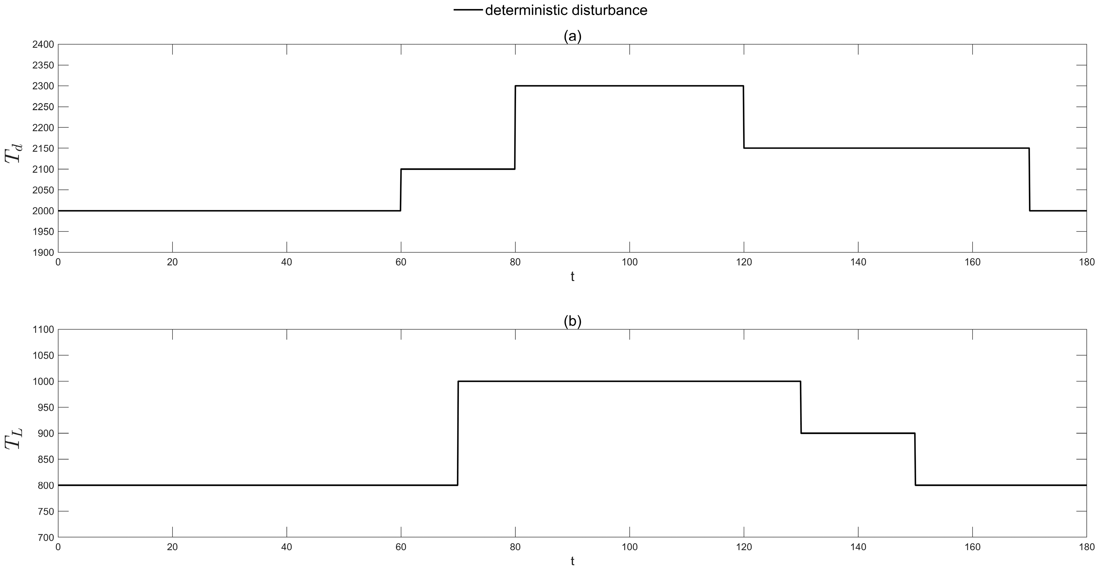
The linear models of both primary and secondary regulations were derived from linearizing the nonlinear mathematical model in Equation (4) about the operating points [34]. The states are p , ω m , and ω p ; inputs are D p and D m ; output is stroke, i s , which is the ratio of ω m to ω p . D p and D m fall within the ranges of 0–147 and 68–160 cm3, respectively. T d and T L are kept constant as 2000 and 800 Nm, respectively, as in the previous study [34]. The deterministic and stochastic torque values are the average probable values assigned from Carlsson [8]. The values of the other HST parameters can be found in Table 1.
The variability of volumetric efficiencies presents a challenge, as the pump’s efficiency is defined at a fixed speed (2100 rpm), while its typical operation occurs at a lower range (1100–1600 rpm). In contrast, motor efficiency changes with its rotation speed, only becoming consistent at high speeds when displacement is reduced. Rotational dependency adjustments were made between the pump and motor to address these inconsistencies. This was accomplished using two-dimensional lookup tables that feature a consistent structure for both components, as shown in Table 2 and Table 3 [8].
Processor-in-the-Loop (PIL) simulation is a method where a laptop simulates a nonlinear plant, while the control algorithm runs on a dedicated target processor. This study uses a BeagleBoard (beagleboard.org) BeagleBone Black, a compact, cost-effective board featuring an AM335x ARM Cortex-A8 processor running at 1 GHz, 512 MB of DDR3 RAM, and 4 GB of on-board eMMC flash storage [43]. Communication between the laptop and the board is established via a USB–serial link. This approach is valuable because it allows for the direct evaluation of a control algorithm’s performance on the actual hardware, considering real-world constraints like limited memory and specific code behavior. Unlike standard simulations, PIL simulation tests the object code itself, enabling verification of real code behavior, assessment of code coverage, and measurement of execution time. It is crucial to understand that PIL simulation does not run in real time, as communication delays between the laptop and the hardware are often more critical than computation time. The method can also identify performance deviations that arise from the compilation process by comparing the model’s behavior with that of the deployed code [44].
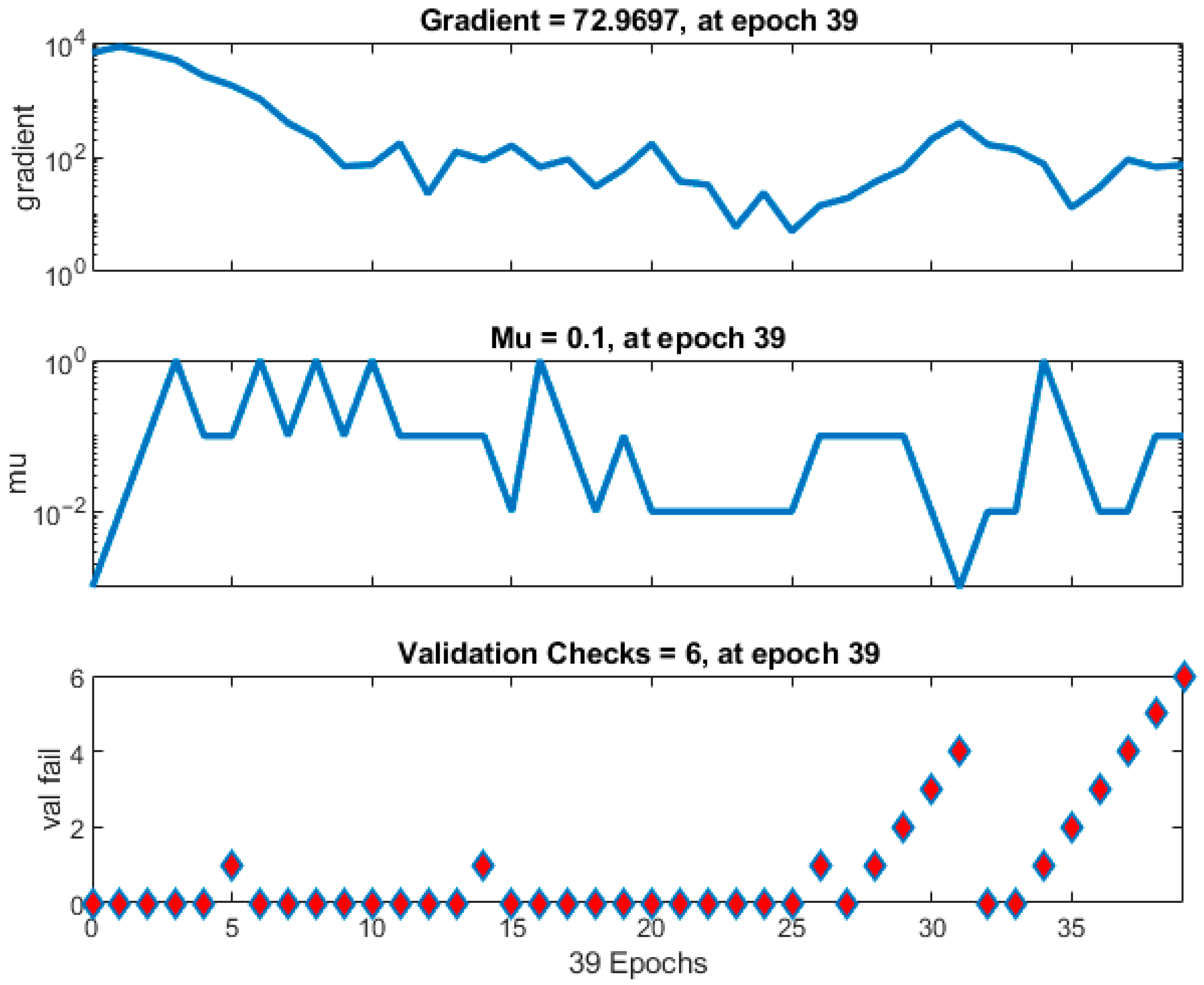
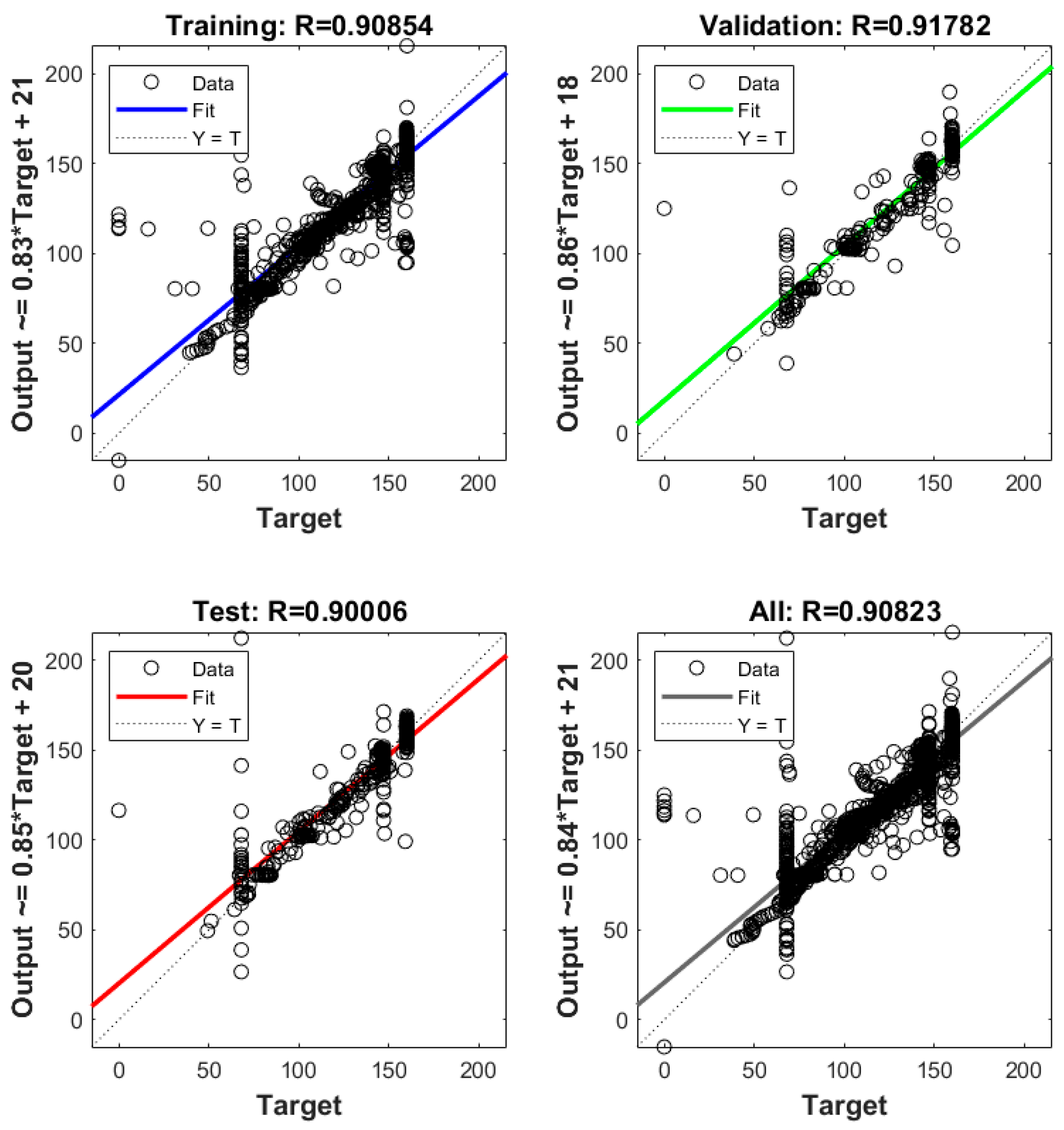
The proposed ANN controller was designed to achieve desired and controlled primary and secondary regulation for the HST, performing this function like the Multiple MPC, whose design step details were given in the previous study [34]. The data of the Multiple MPC was collected from the simulations carried out in terms of the closed-loop nonlinear model of the HST in MATLAB R2024b Simulink with a sampling period of 0.1s. The Multiple MPC has two inputs, the i s value along with its reference, and two outputs, D p and D m . Then, the collected double input–double output dataset, comprising 1800 datapoints for each variable, was normalized with center data to have a mean of 0 and organized into 70% for training, 15% for validation, and 15% for testing, as shown in Table 4. The Levenberg–Marquardt backpropagation algorithm and five hidden neurons were selected through trial and error, as they provide the best balance between minimizing error and maintaining computational efficiency for ANN training. The activation functions of the hidden and output layers were chosen as tangent sigmoid and linear, respectively. The damping factor, μ , was initially selected as 0.001. As a result of the trained ANN, μ was obtained as 0.1 at 39 epochs (Figure 3); the average value of R 2 was approximately 0.9 and the average MSE was about 200 (Figure 4 and Figure 5) for training, validation, and testing.
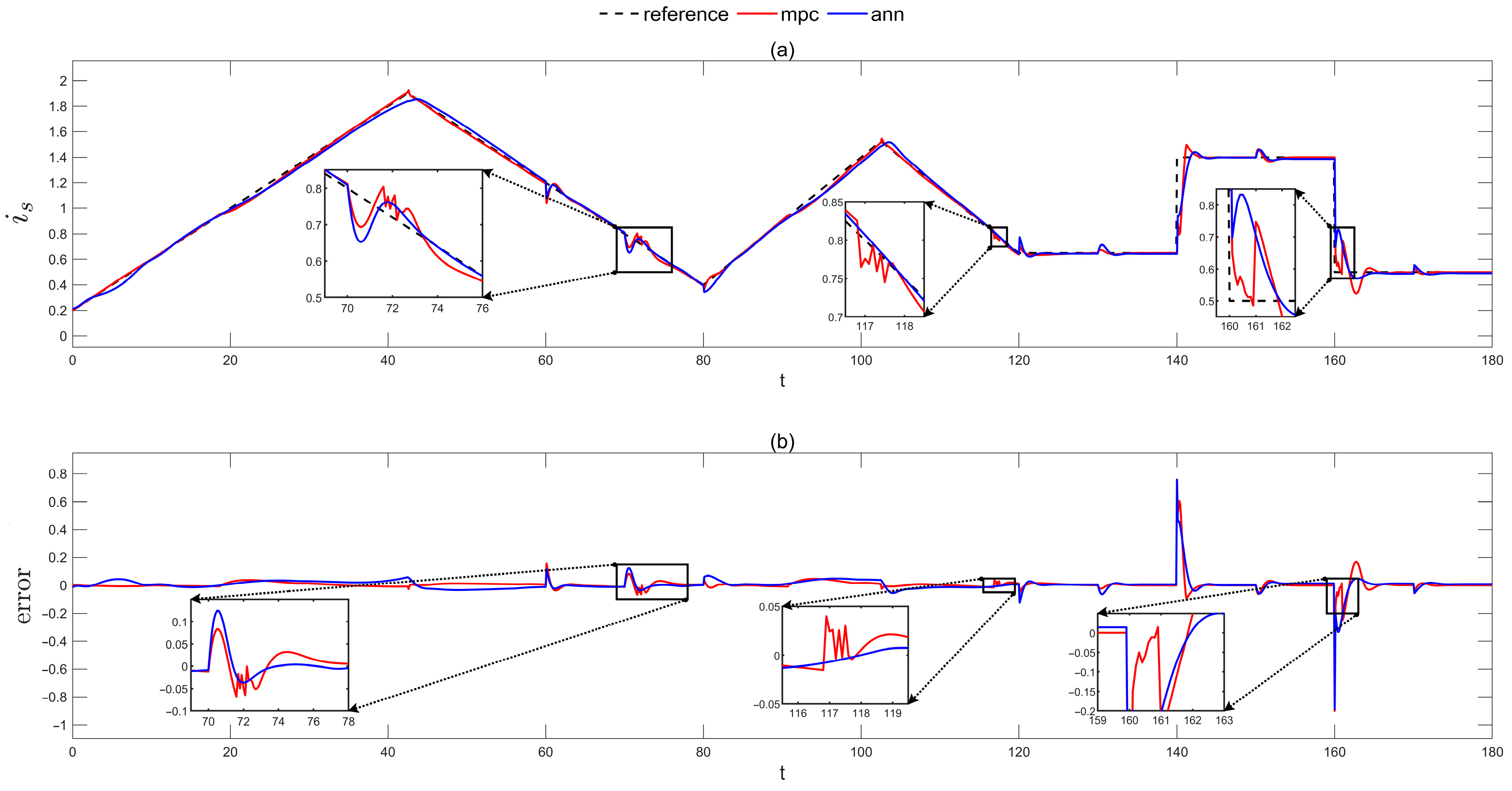
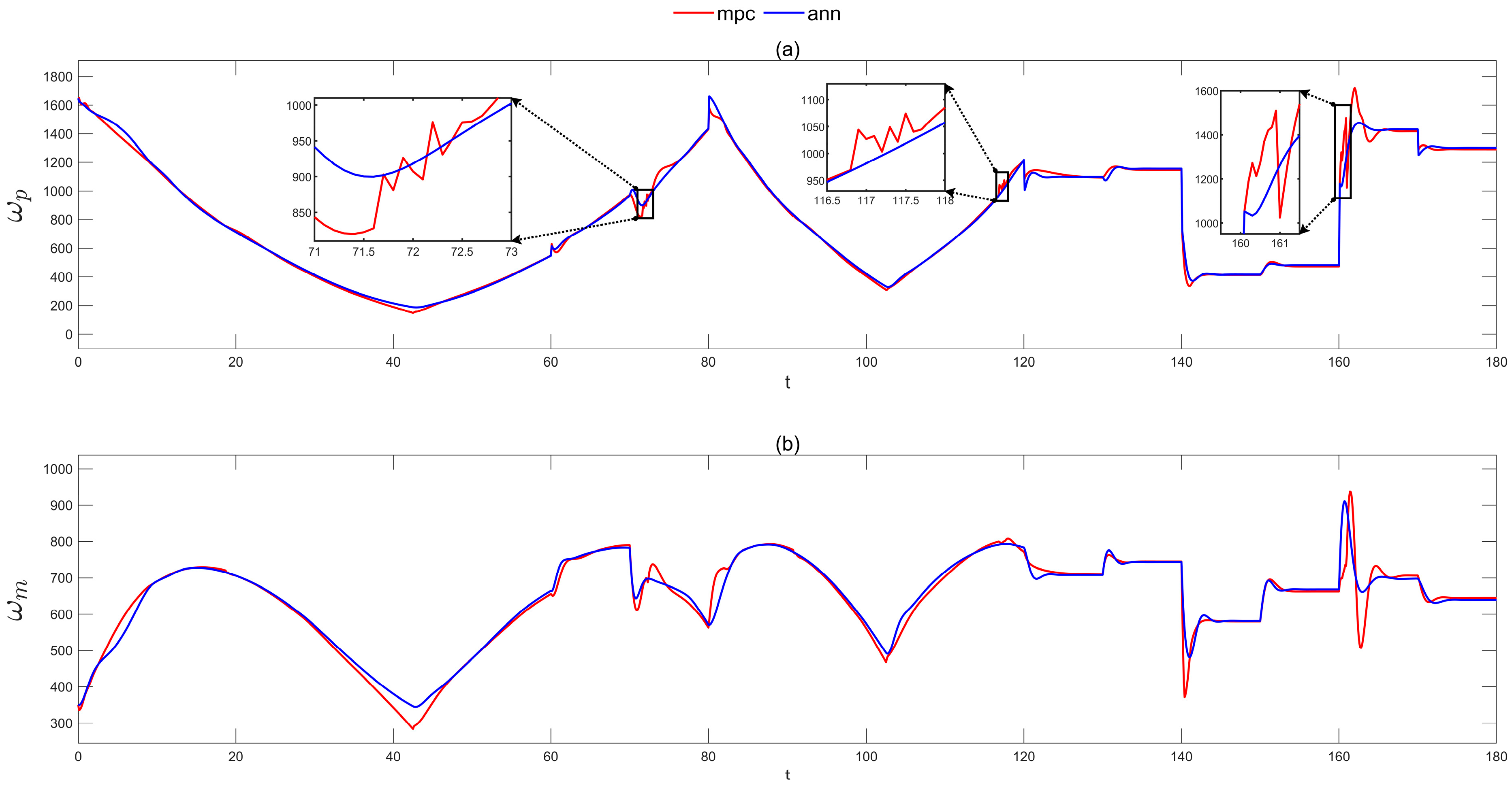
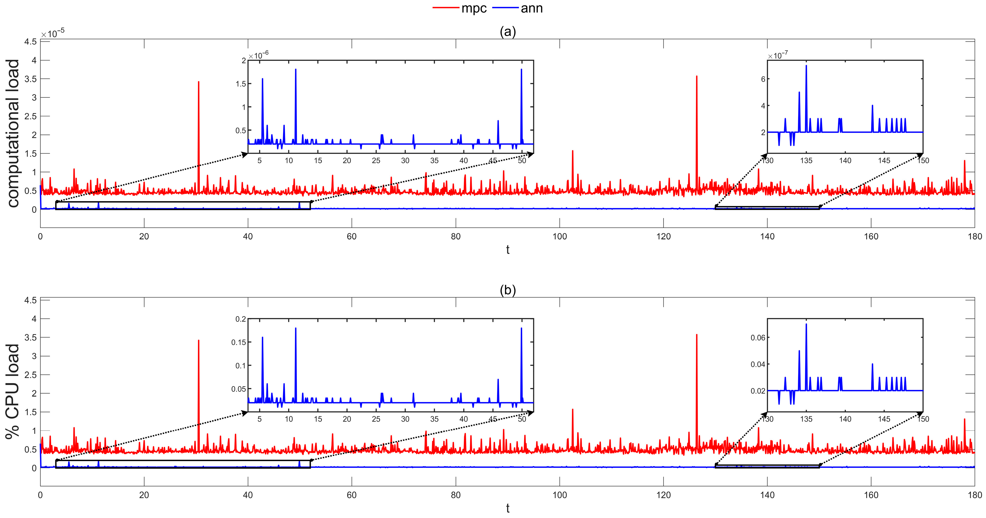
First, the performance of the ANN and Multiple MPCs was evaluated using the closed-loop nonlinear time-varying model of the HST in Figure 6 under the complex trajectory and deterministic disturbances. The goal was to track the reference trajectories of the primary and secondary regulations. The deterministic disturbances in Figure 7 were modeled by a series of changes, including a T d shift from 2000 to 2300 Nm, a T L change from 800 to 1000 Nm, and the reference of i s change from 0.2 to 1.9 using a combination of step and ramp functions. These scenarios were simulated for 180 s in MATLAB R2024b using a stiff differential equation solver [34]. The graphs detailing all the results, including the error between stroke reference, i s , r e f , and i s , and computational loads along with percentage CPU loads of these PIL simulations are presented in Figure 8, Figure 9, Figure 10, Figure 11 and Figure 12.
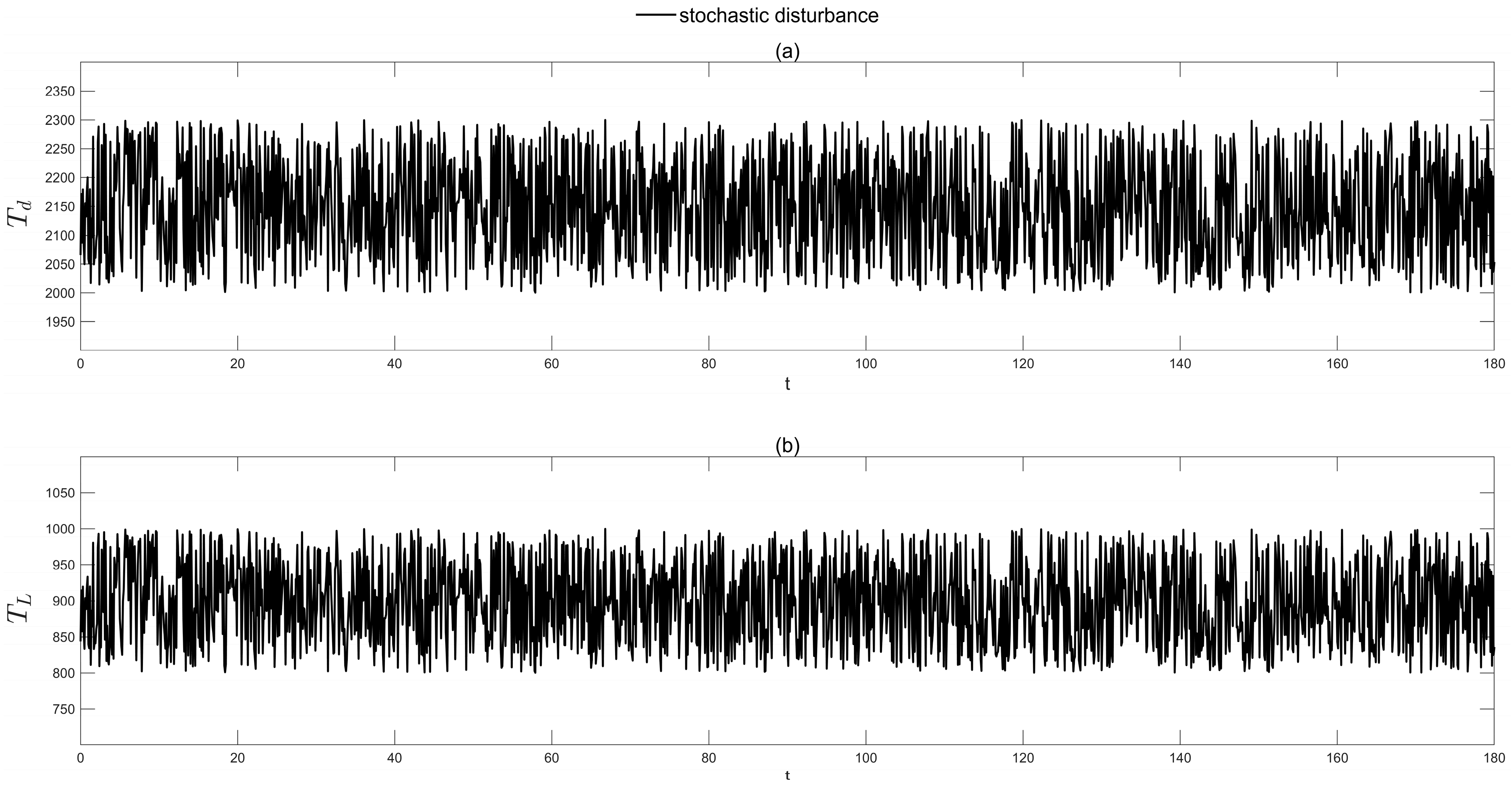
Finally, the performance of the ANN and Multiple MPCs was evaluated using the same complex trajectory as the first scenario, but this time with stochastic disturbances. These disturbances were simulated using uniformly distributed random numbers at a frequency of 1 kHz, applied to T d ranges of 2000–2300 Nm and T L 800–1000 Nm, as shown in Figure 13. Then, the closed-loop nonlinear models were simulated for 180 s in MATLAB R2024b using a stiff differential equation solver [34]. The results of these PIL simulations, including the error between i s , r e f and i s and the computational and percentage CPU loads can be found in Figure 14, Figure 15, Figure 16, Figure 17 and Figure 18.
From Figure 8 and Figure 14, the percentage maximum overshoot (MO), peak time ( t p ), and Mean Squared Error (MSE) were calculated for the PIL simulations under both deterministic and stochastic disturbances, with the results presented in Table 5 and Table 6.
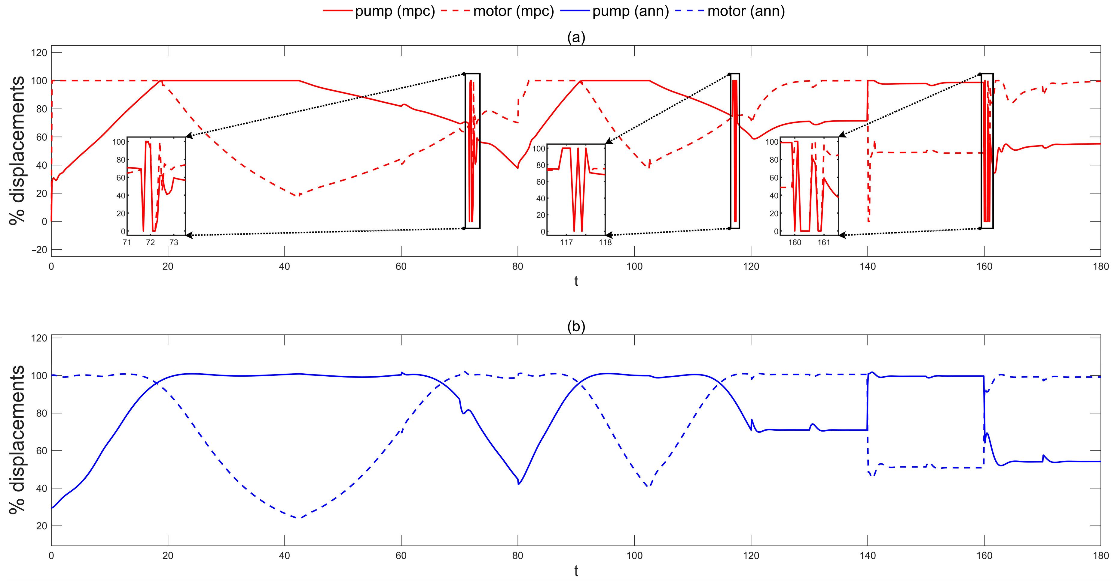
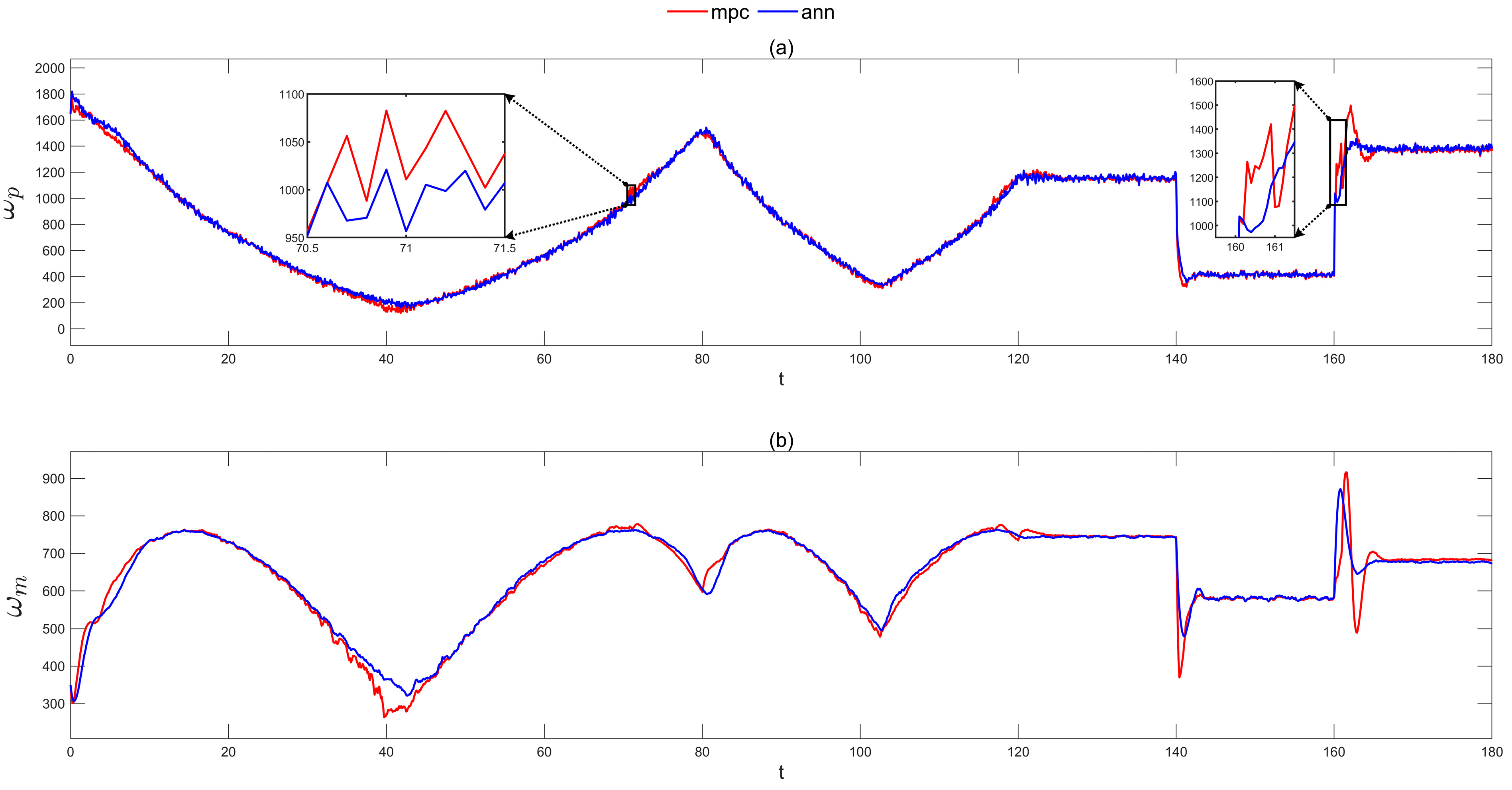
The closed-loop system with the ANN controller exhibits lower MO and MSE values compared to the Multiple MPC during the PIL simulations for both deterministic and stochastic disturbances, as shown in Table 5 and Table 6. It can be clearly seen in Figure 8 and Figure 14 that the proposed ANN controller has a superior reference tracking ability and is insensitive to parameter changes. Due to the change in volumetric efficiencies and, consequently, the angular speeds of the pump and motor in Figure 9, Figure 10, Figure 15 and Figure 16, MOs, particularly for the Multiple MPC, occurred more frequently than with the ANN controller. Also, from the zoom images in Figure 8, Figure 9, Figure 10, Figure 11, Figure 15, Figure 16 and Figure 17, it is concluded that the Multiple MPC causes more oscillatory responses than the ANN controller. The proposed controller, which can reject both deterministic disturbances (Figure 7) and stochastic disturbances (Figure 13), is superior to the Multiple MPC scheme.
The metrics for controller effort, namely Average Effort (AE), Maximum Effort (ME), Average Computational Load (CL), and percentage Average CPU Load (ACPUL), were obtained from PIL simulations for both deterministic and stochastic disturbances, with the results presented in Table 7 and Table 8.
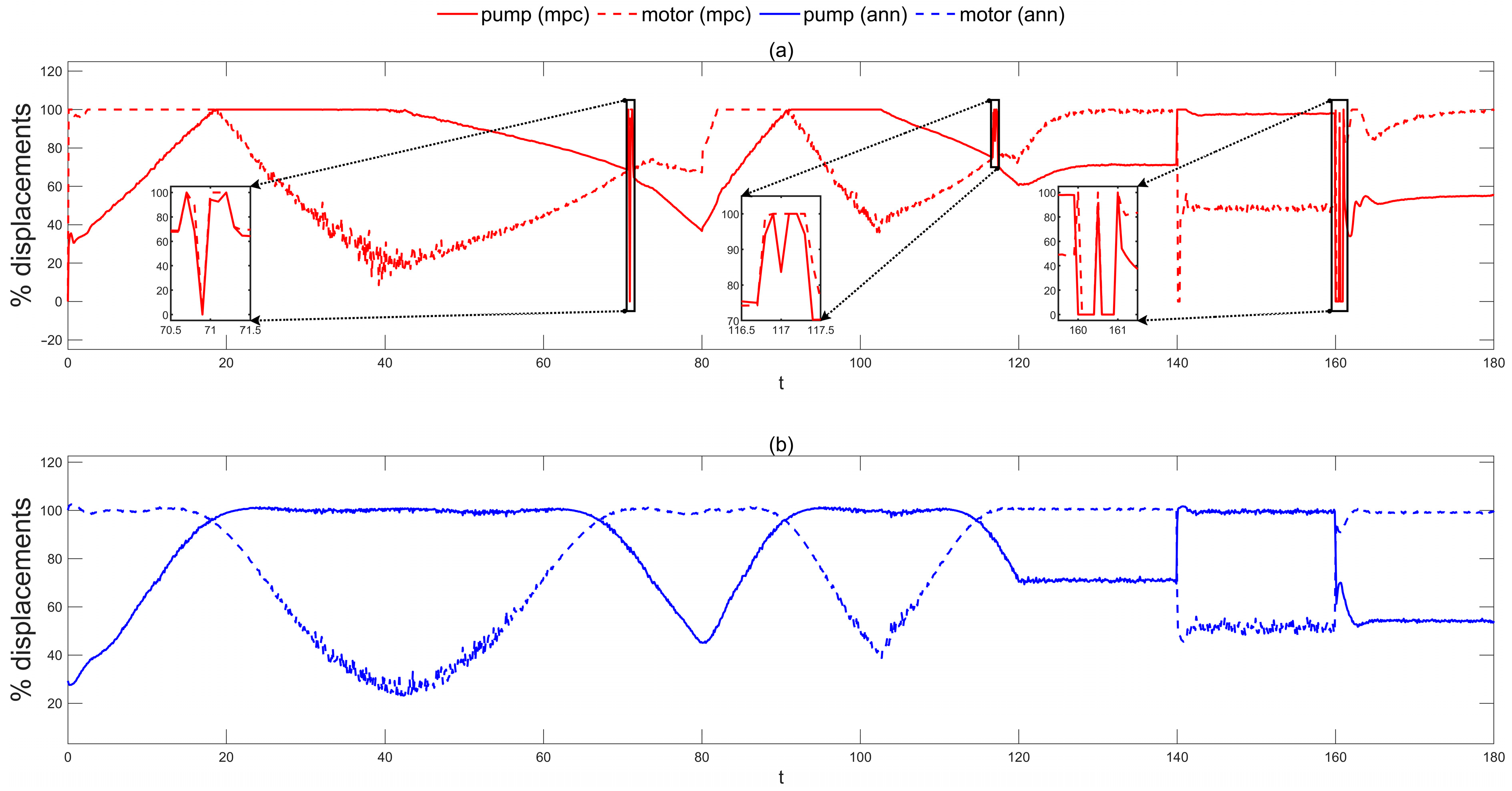
Based on the data from Table 7 and Table 8 and Figure 11, Figure 12, Figure 17 and Figure 18, the ANN controller demonstrates a lower average control effort and computational and CPU loads, indicating a smoother, more energy-efficient control strategy under both deterministic and stochastic disturbances. In contrast, the Multiple MPC operates with a higher average effort; the computational and CPU loads reflecting a more aggressive control approach in terms of high-frequency oscillating behaviour that consumes significantly more energy. Ultimately, the ANN controller provides a higher relative stability and a more energy-efficient control strategy that adapts better to new conditions than the Multiple MPC.
The PIL simulations conducted in this study confirmed the absence of both computational errors and communication delays. This was evidenced by the consistent zero difference between the control inputs of the software model and the object code running on the hardware. Also, the performance of the ANN controller was observed to be better compared with the Multiple MPC in terms of lower ACL and %ACPUL in Table 7 and Table 8. Consequently, these findings validate that the BeagleBone Black was an appropriate choice for the target hardware.
Based on the results of the PIL simulations, the new proposed ANN controller was found to be highly effective. It successfully tracked a complex reference trajectory under the disturbances and the time-varying parameter changes, exhibiting small MO and MSE values and admissible t p values compared to the Multiple MPC scheme, which determined optimal D p and D m parameters for primary and secondary regulations.
The proposed ANN controller functions as a data-driven surrogate model trained on data generated by the Multiple MPC scheme. This approach is designed to replicate the robust performance of the computationally intensive MPC while offering significant benefits in real-time implementation. The core finding is that this computationally efficient ANN can achieve comparable, and in some cases superior, performance. The ANN’s enhanced ability to reject both deterministic and stochastic disturbances is attributed to its training on a dataset that already captures the system’s behavior under these conditions. By learning from this empirical data, the ANN develops an implicit understanding of how to compensate for disturbances, bypassing the need for a real-time optimization solver. This learned model is inherently more robust to real-world uncertainties like parameter drift and noise compared to a rigid, model-based optimization approach. The ANN effectively generalizes from the training data, smoothing out random fluctuations and accommodating minor parameter variations that could cause instability in a conventional controller.

6. Conclusions

Stroke control for the HST of off-road vehicles, such as tractors and forest vehicles, is critical for speed regulation. Still, it is challenging to manage due to external disturbances like varying soil and road conditions. Conventional controllers often fail to provide satisfactory performance because of their sensitivity to these disturbances. In this study, a new control strategy was proposed: an ANN controller for HST stroke control. The proposed ANN controller acts as a data-driven surrogate model for the Multiple MPC scheme, effectively replicating its performance with significant computational advantages. By learning from a dataset that includes the effects of both deterministic and stochastic disturbances, the ANN gains an implicit robustness that allows it to handle real-world uncertainties like noise and parameter drift more efficiently than the optimization-based MPC, making it a convenient alternative for real-time applications. Its performance was compared against a Multiple MPC controller designed in the previous study [34]. The ANN controller proved effective at handling unmeasured disturbances, such as engine and load torques, which was verified through PIL simulations. These simulations confirmed the practical viability of the controller and the chosen hardware, the BeagleBone Black. The implemented ANN controller demonstrated robustness by successfully managing multiple reference changes, variable pump and motor efficiencies, and both deterministic and stochastic disturbances while tracking complex trajectories. The results from the PIL simulations were highly encouraging, showing that the proposed ANN controller is a better option than the Multiple MPC scheme, particularly in terms of lower MO, AE, and MSE values, which are superior to those of the Multiple MPC scheme for real-time HST applications in terms of simplicity and computational cost-effectiveness.
The novelty of this study lies in proposing the ANN controller, trained on Multiple MPC data, that demonstrates superior performance, greater energy efficiency, and verified robustness on hardware via PIL simulations, extending beyond the previous study [34]. The proposed ANN controller offers an ideal solution for off-road vehicles, where cost and hardware constraints are significant, as it requires lower energy consumption and less computational power. Furthermore, this study’s success demonstrates the potential of artificial neural networks for solving other complex control problems in hydraulic systems. This methodology’s proven ability to handle complex trajectories and disturbances makes it applicable for use far beyond forest vehicles, offering significant potential for critical applications like military tracked vehicles and marine propulsion.
Future research will involve designing intelligent controllers using other learning algorithms available in the literature, with a primary focus on maximizing relative stability, accuracy, and disturbance rejection capabilities and minimizing the energy consumption of the closed-loop system.

Funding

This research received no external funding.

Conflicts of Interest

The author declares no conflict of interest.

References

  1. Merritt, H.E. Hydraulic Control System; John Wiley & Sons: New York, NY, USA, 1991. [Google Scholar]
  2. Zarotti, L.G. Hydrostatic Transmissions: Single Directive Control Architectures. Int. J. Model. Simul. 1992, 12, 97–101. [Google Scholar] [CrossRef]
  3. Weisenbach, C.O. Hydrostatic transmission applications. In SAE Technical Papers; SAE International: Warrendale, PA, USA, 1968; pp. 1–8. [Google Scholar]
  4. Wu, K.; Zhang, Q.; Hansen, A. Modelling and identification of a hydrostatic transmission hardware-in-the-loop simulator. Int. J. Veh. Des. 2004, 34, 52–64. [Google Scholar] [CrossRef]
  5. Cundiff, J.S. Fluid Power Circuits and Controls: Fundamentals and Applications; CRC Press LLC: New York, NY, USA, 2001. [Google Scholar]
  6. Dasgupta, K. Analysis of a hydrostatic transmission system using low speed high torque motor. Mech. Mach. Theory 2000, 35, 1481–1499. [Google Scholar] [CrossRef]
  7. Nikranjbar, A.; Sharbabaki, A.N. Simulation and Control of Wind Turbine using Hydrostatic Drive Train. Majlesi J. Energy Manag. 2013, 2, 12–17. [Google Scholar]
  8. Carlsson, E. Modeling Hydrostatic Transmission in Forest Vehicle; Linkopings Universitet: Linköping, Sweden, 2006. [Google Scholar]
  9. Maciejowski, J.M. Predictive Control with Constraints; Prentice Hall: London, UK, 2002. [Google Scholar] [CrossRef]
  10. Ding, Y.; Wang, L.; Li, Y.; Li, D. Model predictive control and its application in agriculture: A review. Comput. Electron. Agric. 2018, 151, 104–117. [Google Scholar] [CrossRef]
  11. Coen, T.; Saeys, W.; Missotten, B.; De Baerdemaeker, J. Cruise control on a combine harvester using model-based predictive control. Biosyst. Eng. 2008, 99, 47–55. [Google Scholar] [CrossRef]
  12. Sun, H.; Meinlschmidt, T.; Aschemann, H. Comparison of two nonlinear model predictive control strategies with observer-based disturbance compensation for a hydrostatic transmission. In Proceedings of the 2014 19th International Conference on Methods and Models in Automation and Robotics, MMAR 2014, Miedzyzdroje, Poland, 2–5 September 2014; pp. 526–531. [Google Scholar]
  13. Dutta, A.; lonescu, C.; De Keyser, R. A pragmatic approach to distributed nonlinear model predictive control: Application to a hydrostatic drivetrain. Optim. Control. Appl. Methods 2015, 36, 369–380. [Google Scholar] [CrossRef]
  14. Backas, J.; Ghabcheloo, R. Nonlinear model predictive energy management of hydrostatic drive transmissions. Proc. Inst. Mech. Eng. Part I J. Syst. Control Eng. 2019, 233, 335–347. [Google Scholar] [CrossRef]
  15. Vu, T.-V.; Chen, C.-K.; Hung, C.-W. A model predictive control approach for fuel economy improvement of a series hydraulic hybrid vehicle. Energy 2014, 7, 7017–7040. [Google Scholar] [CrossRef]
  16. Vu, T.-V.; Chen, C.-K. A Model-Based Controller Development for a Series Hydraulic Hybrid Vehicle. In AETA 2016 Recent Advances in Electrical Engineering and Related Sciences; Lecture Notes in Electrical Engineering; Springer; Cham, Switzerland; pp. 891–901.
  17. Deppen, T.O.; Alleyne, A.G.; Stelson, K.A.; Meyer, J.J. Optimal energy use in a light weight hydraulic hybrid passenger vehicle. J. Dyn. Syst. Meas. Control Trans. ASME 2012, 134, 041009. [Google Scholar] [CrossRef]
  18. Nawrocka, A.; Kwaśniewski, J. Predictive neural network controller for hydrostatic transmission control. Mech./AGH Univ. Sci. Technol. 2008, 27, 62–65. [Google Scholar]
  19. Narendra, K.S.; Parthasarathy, K. Identification and control of dynamical systems using neural networks. IEEE Trans. Neural Netw. 1990, 1, 4–27. [Google Scholar] [CrossRef]
  20. Kaluz, M.; Kohut, R.; Dzurkova, D. MPC-Mimicking Neural Network Based on Homomorphic Encryption. In Proceedings of the 2023 24th International Conference on Process Control (PC), Strbske Pleso, Slovakia, 6–9 June 2023; pp. 126–131. [Google Scholar]
  21. Novak, M.; Dragicevic, T. Supervised imitation learning of finite-set model predictive control systems for power electronics. IEEE Trans. Ind. Electron. 2021, 68, 1717–1723. [Google Scholar] [CrossRef]
  22. Subramanian, S.B.; Sisay, Z.; Azath, M.; Girma, Y. Design and implementation of an ANN-based MPPT controller for solar-powered BLDC motor systems: A case study in Yalo Lala village, Ethiopia. Eng. Res. Express 2025, 7, 025301. [Google Scholar] [CrossRef]
  23. Abdullah, A.G.; Ibrahim, M.A.; Salih, A.S. Performance Enhancing Speed Control of a DC Motor Based on an Artificial Neural Network. J. Eur. Des Systèmes Autom. 2024, 57, 1489–1495. [Google Scholar] [CrossRef]
  24. Mahmoud, I.; Khedher, A. Artificial Neural Network-based Control of a Switched Reluctance Motor for a High-precision Positioning System. Eng. World 2024, 6, 136–143. [Google Scholar] [CrossRef]
  25. Abdolrasol, M.G.M.; Hannan, M.A.; Hussain, S.M.S.; Ustun, T.S.; Sarker, M.R.; Ker, P.J. Energy Management Scheduling for Microgrids in the Virtual Power Plant System Using Artificial Neural Networks. Energies 2021, 14, 6507. [Google Scholar] [CrossRef]
  26. Schöning, J.; Riechmann, A.; Pfisterer, H.J. AI for Closed-Loop Control Systems: New Opportunities for Modeling, Designing, and Tuning Control Systems. In Proceedings of the ICMLC 2022: 2022 14th International Conference on Machine Learning and Computing, Guangzhou, China, 18–21 February 2022; pp. 1–11. [Google Scholar]
  27. Rafiuddin, N.; Khan, Y.U. Nonlinear controller design for mechatronic aeropendulum. Int. J. Dyn. Control. 2023, 11, 1662–1670. [Google Scholar] [CrossRef]
  28. Antão, R.; Antunes, J.; Mota, A.; Martins, R.E. Model Predictive Control of Non-Linear Systems Using Tensor Flow-Based Models. Appl. Sci. 2020, 10, 3958. [Google Scholar] [CrossRef]
  29. Bana, P.R.; D’arco, S.; Amin, M. ANN-Based Robust Current Controller for Single-Stage Grid-Connected PV with Embedded Improved MPPT Scheme. IEEE Access 2024, 12, 100251–100262. [Google Scholar] [CrossRef]
  30. Shneen, S.W.; Gaber, R.K.; Salih, R.S.; Jiaad, S.M. Artificial Neural Network (ANN) Based Proportional Integral Derivative (PID) for Arm Rehabilitation Device. Kufa J. Eng. 2025, 16, 80–103. [Google Scholar] [CrossRef]
  31. Mishra, S.K.; Singh, P.K. Modeling of a Closed Loop Hydrostatic Transmission System and Its Control Designed for Automotive Applications. In Advances in Engine Tribology. Energy, Environment, and Sustainability; Kumar, V., Agarwal, A.K., Jena, A., Upadhyay, R.K., Eds.; Springer: Berlin/Heidelberg, Germany, 2022; pp. 219–238. [Google Scholar]
  32. Ji, Y.; Huang, Y.; Yang, M.; Leng, H.; Ren, L.; Kiu, H.; Chen, Y. Physics-informed deep learning for virtual rail train trajectory following control. Reliab. Eng. Syst. Saf. 2025, 261, 111092. [Google Scholar] [CrossRef]
  33. Ramos-Martinez, M.; Torres-Cantero, C.A.; Ortiz-Torres, G.; Sorcia-Vázquez, F.D.J.; Avila-George, H.; Lozoya-Ponce, R.E.; Vargas-Méndez, R.A.; Renteria-Vargas, E.M.; Rumbo-Morales, J.Y. Control for Bioethanol Production in a Pressure Swing Adsorption Process Using an Artificial Neural Network. Mathematics 2023, 11, 3967. [Google Scholar] [CrossRef]
  34. Ülker, H. Design and application of multiple model predictive control in stroke control of hydrostatic transmission. Adv. Mech. Eng. 2025, 17, 16878132251331720. [Google Scholar] [CrossRef]
  35. Zavadinka, P.; Kriššák, P. Simulation of vehicle working conditions with hydrostatic pump and motor control algorithm. J. Autom. Mob. Robot. Intell. Syst. 2012, 6, 40–46. [Google Scholar]
  36. Stosiak, M.; Karpenko, M.; Prentkovskis, O.; Deptuła, A.; Skackauskas, P. Research of vibrations effect on hydraulic valves in military vehicles. Def. Technol. 2023, 30, 111–125. [Google Scholar] [CrossRef]
  37. Stosiak, M.; Karpenko, M.; Deptuła, A.; Urbanowicz, K.; Skačkauskas, P.; Deptuła, A.M.; Danilevičius, A.; Šukevičius, Š.; Łapka, M. Research of Vibration Effects on a Hydraulic Valve in the Pressure Pulsation Spectrum Analysis. J. Mar. Sci. Eng. 2023, 11, 301. [Google Scholar] [CrossRef]
  38. Stosiak, M.; Yatskiv, I.; Prentkovskis, O.; Karpenko, M. Reduction of Pressure Pulsations over a Wide Frequency Range in Hydrostatic Systems. Machines 2025, 13, 25. [Google Scholar] [CrossRef]
  39. Bemporad, A.; Lawrence Ricker, N.; Morari, M. Model Predictive Control ToolboxTM Reference How to Contact MathWorks—R2020a; MathWorks: Natick, MA, USA, 2020; p. 994. [Google Scholar]
  40. Beale, M.H.; Hagan, M.T.; Demuth, H.B. Deep Learning Toolbox TM User’s Guide; R2024b; The MathWorks, Inc.: Natick, MA, USA, 2024. [Google Scholar]
  41. Hagan, M.T.; Demuth, H.B.; Beale, M.H.; De Jesús, O. Neural Network Design; Martin Hagan: Stillwater, OK, USA, 2014. [Google Scholar]
  42. Levenberg, K. A Method for the Solution of Certain Non-Linear Problems in Least Squares. Q. Appl. Math. 1944, 2, 164–168. [Google Scholar] [CrossRef]
  43. BeagleBoard. What İs BeagleBone Black? Available online: https://www.beagleboard.org/boards/beaglebone-black (accessed on 31 July 2025).
  44. Ülker, H.; Baykara, C.; Özsoy, C. PIL simulations of an FWUAV under windy conditions. Aircr. Eng. Aerosp. Technol. 2018, 90, 461–470. [Google Scholar] [CrossRef]
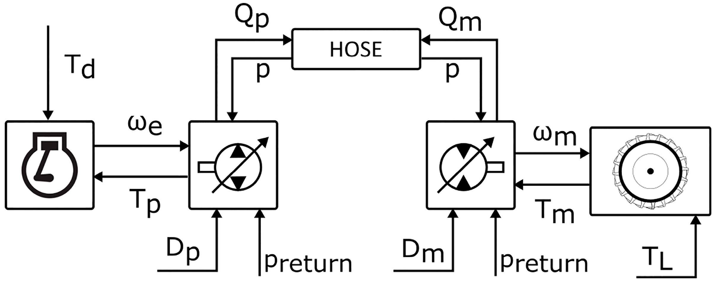
Figure 1. Block diagram of the HST system [34].
Machines 13 00778 g001
Figure 2. ANN flow chart.
Machines 13 00778 g002
Figure 3. Training state values of the trained ANN.
Machines 13 00778 g003
Figure 4. Regression values of the trained ANN.
Machines 13 00778 g004
Figure 5. Best validation performance in terms of MSE values of the trained ANN.
Machines 13 00778 g005
Figure 6. Block diagram created in MATLAB R2024b Simulink of the closed-loop system.
Machines 13 00778 g006
Figure 7. Deterministic torque disturbances: (a) T d and (b) T L .
Machines 13 00778 g007
Figure 8. (a) Stroke responses and (b) errors of the closed-loop systems with Multiple MPC and ANN in the case of deterministic torque disturbances.
Machines 13 00778 g008
Figure 9. Angular speeds of the (a) pump and (b) motor of the closed-loop systems with Multiple MPC and ANN in the case of deterministic torque disturbances.
Machines 13 00778 g009
Figure 10. Volumetric efficiencies of the (a) pump and (b) motor of the closed-loop systems with Multiple MPC and ANN in the case of deterministic torque disturbances.
Machines 13 00778 g010
Figure 11. Normalized percentage of pump and motor displacements of the closed-loop systems with (a) Multiple MPC and (b) ANN in the case of deterministic torque disturbances.
Machines 13 00778 g011
Figure 12. (a) Computational and (b) percentage CPU loads in the case of deterministic torque disturbances.
Machines 13 00778 g012
Figure 13. Stochastic torque disturbances: (a) T d and (b) T L .
Machines 13 00778 g013
Figure 14. (a) Stroke responses and (b) errors of the closed-loop systems with Multiple MPC and ANN in the case of stochastic torque disturbances.
Machines 13 00778 g014
Figure 15. Angular speeds of the (a) pump and (b) motor of the closed-loop systems with Multiple MPC and ANN in the case of stochastic torque disturbances.
Machines 13 00778 g015
Figure 16. Volumetric efficiencies of the (a) pump and (b) motor of the closed-loop systems with Multiple MPC and ANN in the case of stochastic torque disturbances.
Machines 13 00778 g016
Figure 17. Normalized percentage of pump and motor displacements of the closed-loop systems with (a) Multiple MPC and (b) ANN in the case of stochastic torque disturbances.
Machines 13 00778 g017
Figure 18. (a) Computational and (b) percentage CPU loads in the case of stochastic torque disturbances.
Machines 13 00778 g018
Table 1. The values of the HST system parameters [8].
System Parameters of HSTUnitValue
J m w Nms25.02
J p d Nms20.1723
K m Nm0
K p Nm0
V m35.98 × 10−4
β Pa3.7 × 106
η t m -0.97
η t p -0.92
μ m Nms5
μ p Nms10
Table 2. Volumetric efficiency for the pump [8].
ω p (rpm)01100135016002500
D p
( c m 3 / r e v )
00.560.560.580.590.59
850.840.840.860.870.87
1470.90.90.920.930.93
Table 3. Volumetric efficiency for the motor [8].
ω m (rpm)0600120020004000
D m
( c m 3 / r e v )
680.770.770.880.970.97
1050.810.810.910.970.97
1600.850.850.940.970.97
Table 4. The parameters of the trained ANN model.
ParameterValue
Input Nodes2
Hidden Layer1
Hidden Layer Neurons5
Hidden Layer Activation FunctionTangent sigmoid
Output Nodes2
Output Layer Activation FunctionLinear
Training Data Percentage70
Validation Data Percentage15
Test Data Percentage15
Training Network AlgorithmLevenberg–Marquardt
Damping Factor0.001
Number of Epochs1000
Validation Checks6
PerformanceMean Squared Error
Table 5. Maximum performance measures of the PIL simulations in the case of deterministic disturbances.
Control StrategyDisturbance ProfileMO (%) t p (s)MSE
Multiple MPCDeterministic (Figure 7)2510.0024
ANNDeterministic (Figure 7)1010.0016
Table 6. Maximum performance measures of the PIL simulations in the case of stochastic disturbances.
Control StrategyDisturbance ProfileMO (%) t p (s)MSE
Multiple MPCStochastic (Figure 13)2410.0048
ANNStochastic (Figure 13)102.80.0039
Table 7. Controller performances during the PIL simulations in the case of deterministic disturbances.
Control StrategyDisturbance ProfileAEMEACL (s)% ACPUL
Multiple MPCDeterministic (Figure 7)0.7914.83 × 10−60.48
ANNDeterministic (Figure 7)0.771.012.08 × 10−70.02
Table 8. Controller performances during the PIL simulations in the case of stochastic disturbances.
Control StrategyDisturbance ProfileAEMEACL (s)% ACPUL
Multiple MPCStochastic (Figure 13)0.7915.7 × 10−60.57
ANNStochastic (Figure 13)0.771.022.14 × 10−70.021
Disclaimer/Publisher’s Note: The statements, opinions and data contained in all publications are solely those of the individual author(s) and contributor(s) and not of MDPI and/or the editor(s). MDPI and/or the editor(s) disclaim responsibility for any injury to people or property resulting from any ideas, methods, instructions or products referred to in the content.