Article

Trajectory Tracking Control for Wheeled Mobile Robots with Unknown Slip Rates Based on Improved Rapid Variable Exponential Reaching Law and Sliding Mode Observer

1
College of Mechanical and Electronic Engineering, Northwest A&F University, Yangling 712100, China
2
Filtang Technologies Corporation, Yantai 264006, China
*
Author to whom correspondence should be addressed.
Machines 2025, 13(9), 765; https://doi.org/10.3390/machines13090765
Submission received: 28 July 2025 / Revised: 17 August 2025 / Accepted: 25 August 2025 / Published: 27 August 2025
(This article belongs to the Section Robotics, Mechatronics and Intelligent Machines)

Abstract

Aiming at the trajectory tracking control problem of wheeled mobile robots under unknown slip ratio conditions, this paper designs a trajectory tracking controller based on an improved rapid variable power reaching law and a sliding mode observer. First, a kinematic model of the wheeled mobile robot is established, explicitly considering the influence of slip ratio. Then, a sliding mode observer is developed for online estimation of the slip ratio, addressing the difficulty of direct slip ratio measurement. On this basis, a trajectory tracking controller is designed based on the improved rapid variable power reaching law, enabling fast tracking of multiple complex trajectories under slip conditions. Simulation and experimental results show that the proposed trajectory tracking controller not only effectively eliminates the influence of unknown slip disturbances on trajectory tracking, improving smoothness and tracking accuracy but also greatly accelerates the convergence process. The shortest convergence time is only 20.56% of that achieved by a fuzzy PID trajectory tracking controller and 61.43% of that achieved by a rapid double power reaching law trajectory tracking controller with a sliding mode observer.

1. Introduction

The rapid advancement of wheeled mobile robot technology has led to their widespread adoption in diverse domains, including domestic services, industrial operations, and space exploration, significantly enhancing both quality of life and scientific research capabilities. To accomplish their designated tasks, wheeled mobile robots must reliably and precisely follow predetermined paths to reach target destinations. Consequently, accurate trajectory tracking has become one of the most fundamental and critical technologies for wheeled mobile robots [1,2].
As a typical nonlinear and complex motion system, a wheeled mobile robot encounters numerous challenges in trajectory tracking due to its operation in diverse and dynamic environments. External factors such as environmental disturbances, tire slippage, and variable ground friction make the design of high-performance trajectory tracking controllers particularly complex. Therefore, achieving high-precision and fast trajectory tracking control requires the development of robust and efficient control strategies [3,4]. To this end, numerous control methods have been proposed both domestically and internationally for the trajectory tracking of wheeled mobile robots, including optimal control [5], sliding mode control [6,7], fuzzy logic control [8,9,10], model predictive control [11,12,13,14], neural network-based control [15,16,17], adaptive control [18,19], backstepping control [20,21], and nonlinear control [22,23]. Among these, sliding mode control [24,25] has demonstrated outstanding performance due to its strong robustness against external disturbances, fast dynamic response, simple structure, and ease of implementation, making it widely adopted in wheeled mobile robot trajectory tracking applications. For example, Lin et al. [26] proposed a global sliding mode tracking controller using a fast power law approach, achieving rapid convergence of velocity and trajectory tracking errors while significantly reducing chattering. Wang et al. [27] developed a novel sliding mode control strategy with a finite-time convergence reaching law, which improved reaching speed and reduced convergence time. Geng et al. [28] combined the backstepping method with hierarchical sliding mode control to ensure robust asymptotic stability of the closed-loop system. However, these studies primarily consider ideal operating conditions. In real-world scenarios, environmental complexities—such as icy roads in winter, wet surfaces on rainy days, or rapid sharp turns—can lead to wheel slip, significantly degrading tracking performance.
To address slip effects, several studies have explored trajectory tracking control under sliding conditions. Wang et al. [29] proposed an active disturbance rejection control strategy capable of accurately observing disturbances, thereby improving robustness and maintaining trajectory tracking performance during slip events. Li et al. [30] developed an anti-saturation fuzzy super-spiral sliding mode control to mitigate slip disturbances, effectively reducing chattering. Jia et al. [31] designed a backstepping controller capable of automatically compensating for unknown wheel slip disturbances, improving tracking accuracy, anti-interference capability, and robustness. Nevertheless, these methods do not explicitly estimate slip parameters in real time or analyze the slip ratio in detail. In summary, this study addresses the critical challenge of trajectory tracking control for wheeled mobile robots operating under unknown slip conditions, where conventional methods often fail to achieve satisfactory accuracy and robustness. The proposed approach introduces two key innovations: (1) an improved rapid variable exponential reaching law-based controller that ensures stable tracking within finite convergence time despite unknown slip ratios, and (2) a sliding mode observer for real-time slip parameter estimation. By integrating these components, the proposed framework achieves rapid convergence of tracking errors to zero, thereby enabling reliable trajectory tracking and motion control, even under significant slip conditions. The control block diagram was shown in Figure 1. The sliding mode observer performs real-time estimation of slip parameters, while the trajectory tracking controller dynamically adjusts the control law based on both the observer’s outputs and the pose errors of the wheeled mobile robot, ensuring that stable tracking can be achieved within a finite convergence time even under unknown slip ratio conditions.
The key innovations of this research are reflected in three aspects:
(1)
Innovative Control Architecture: Unlike the independent design methods of sliding mode observer and approaching law in existing research, the sliding mode state observer and the improved rapid exponential convergence law are integrated into the same control framework in this paper. The observer is used to estimate unmeasurable slip ratios ( S L , S R ) in real time, and the observation results are directly embedded into the control law. The parameters of the improved rapid exponential convergence law are adjusted in real time according to the motion situation. This deep coupling not only achieves adaptive parameter adjustment and disturbance compensation but also maintains high-precision trajectory tracking performance under unknown sideslip conditions.
(2)
Algorithmic Advancements: Proposes a dual-phase adaptive convergence mechanism that simultaneously accelerates convergence speed and effectively suppresses chattering. Designs a novel sliding surface whose structural parameters can be tuned to regulate the convergence rate of pose errors, guaranteeing finite-time convergence.
(3)
Performance Breakthroughs: Both simulations and experimental results validate the proposed method’s rapid convergence characteristics and strong robustness in unknown slip scenarios.

2. Establishment of Kinematic Model of Wheeled Mobile Robot in Slipping State

As shown in Figure 2, it is assumed that the geometric center of the wheeled robot coincides with its center of mass, and the overall coordinate system is established with reference to the geodetic coordinate system. xoy is a local coordinate system, which is established with reference to the robot’s own coordinate system. The geometric center of the vehicle body is represented by the point O(x,y) in the global coordinate system; the θ is the angle between the forward direction of the robot’s head and the positive direction of the X-axis of the overall coordinate system [32]. v is the linear velocity of the robot. When the robot is moving, the wheels on the same side rotate at the same speed, that is, ω 1 = ω 2 = ω L , ω 3 = ω 4 = ω R , let ω L and ω R represent the angular velocities of the left and right sides of the wheel, respectively, and let v L and v R represent the velocities of the left and right wheel centers, respectively.
Under non-slip conditions, the wheel velocities satisfy the following:
v L = r ω L v R = r ω R
where r is the radius of the wheel. From the kinematic relationships in Figure 2:
v = v L + v R 2 θ ˙ = ω = v L v R b
In the global coordinate system, the kinematic equation of the robot in the absence of slippage can be expressed as follows:
X ˙ Y ˙ θ ˙ = cos θ 0 sin θ 0 0 1 v ω
When the robot slides longitudinally, v L and v R represent the longitudinal velocities of the left and right wheel centers, respectively, and the following relationship holds:
s L = r ω L v L r ω L s R = r ω R v R r ω R
where s L and s R represent the longitudinal slip rates of the left and right wheels, respectively.
By combining Figure 2 and Equation (2), the following can be obtained:
v = v L + v R 2 = r ω L ( 1 s L ) + r ω R ( 1 s R ) 2 ω = θ ˙ = v L v R b = r ω L ( 1 s L ) r ω R ( 1 s R ) b
In the global coordinate system, the kinematic equation of the robot under longitudinal slip [33] can be expressed as follows:
X ˙ Y ˙ θ ˙ = r ω L ( 1 s L ) + r ω R ( 1 s R ) 2 cos θ r ω L ( 1 s L ) + r ω R ( 1 s R ) 2 sin θ r ω L ( 1 s L ) r ω R ( 1 s R ) b
When the robot slides sideways, its speed is not aligned with its forward direction (as indicated by v in Figure 1). The angle between them is denoted as α , and σ is defined as the robot’s sideways slip ratio, leading to the following equations [34]:
σ = tan α .
y ˙ = x ˙ σ = x ˙ tan α .
In the local coordinate system, the kinematic equation describing the robot’s slip motion is given by the following:
x ˙ y ˙ θ ˙ = r ω L ( 1 s L ) + r ω R ( 1 s R ) 2 r ω L ( 1 s L ) + r ω R ( 1 s R ) 2 σ r ω L ( 1 s L ) r ω R ( 1 s R ) b
The transformation between the global and local coordinate systems can be expressed as follows:
X ˙ Y ˙ θ ˙ = cos θ sin θ 0 sin θ cos θ 0 0 0 1 x ˙ y ˙ θ ˙
Combining Equations (6), (9) and (10) yields the kinematic equations in the global coordinate system for the case when the robot experiences both longitudinal and lateral sliding simultaneously:
X ˙ Y ˙ θ ˙ = cos θ + σ sin θ 0 sin θ σ cos θ 0 0 1 v ω
That is:
X ˙ Y ˙ θ ˙ = r ω L ( 1 s L ) + r ω R ( 1 s R ) 2 ( cos θ + σ sin θ ) r ω L ( 1 s L ) + r ω R ( 1 s R ) 2 ( sin σ σ cos θ ) r ω L ( 1 s L ) r ω R ( 1 s R ) b

3. Estimation of Slippage Parameters

3.1. Design of Sliding Mode Observer

When the wheeled robot moves on ice or smooth ground, the wheels are particularly easy to slip. Because the slip parameters are not measurable, the trajectory tracking control effect of the robot in the slip state is poor. To solve these problems, a sliding mode observer is designed to estimate the sliding parameters. Let
M = r ω L ( 1 s L ) + r ω R ( 1 s R ) 2
Then Equation (12) can be expressed as follows:
X ˙ = M ( cos θ + σ sin θ ) Y ˙ = M ( sin θ σ cos θ ) θ ˙ = 2 M b 2 r b ω R ( 1 s R )
The angular velocity of the wheeled robot can be written as follows:
θ ˙ 1 = 2 M b + 2 r b ω L ( 1 s L )
and θ ˙ 1 = θ ˙ .
The system dynamics can be reformulated as follows:
X ˙ = M ( cos θ + σ sin θ ) θ ˙ = 2 M b 2 r b ω R ( 1 s R ) θ ˙ 1 = 2 M b + 2 r b ω L ( 1 s L )
Based on Equation (15), the sliding mode observer is designed as follows:
X ^ ˙ = M cos θ + L 1 sgn ( X X ^ ) + L 2 ( X X ^ ) θ ^ ˙ = 2 M b + L 3 sgn ( θ θ ^ ) + L 2 ( θ θ ^ ) θ ^ ˙ 1 = 2 M b + L 4 sgn ( θ θ ^ 1 ) + L 2 ( θ θ ^ 1 )
where L i > 0 ( i = 1,2 , 3,4 ) are sliding mode observer gains; θ ^ ˙ , θ ^ ˙ 1 are observed values of robot angular velocity.
The observation error dynamics are defined as follows. By combining Equations (15) and (16), the following is obtained:
X ~ ˙ = M σ sin θ L 1 sgn ( X X ̑ ) L 2 ( X X ^ ) θ ~ ˙ = 2 r b ω R ( 1 s R ) L 3 sgn ( θ θ ^ ) L 2 ( θ θ ^ ) θ ~ ˙ 1 = 2 r b ω L ( 1 s L ) L 3 sgn ( θ θ ^ 1 ) L 2 ( θ θ ^ 1 )
The primary function of the sliding mode observer is to ensure finite-time convergence of the observation error. According to Equation (17), the following relationship holds:
M σ sin θ L 1 sgn ( X X ̑ ) L 2 ( X X ^ ) 0 2 r b ω R ( 1 s R ) L 3 sgn ( θ θ ^ ) L 2 ( θ θ ^ ) 0 2 r b ω L ( 1 s L ) L 4 sgn ( θ θ ^ 1 ) L 2 ( θ θ ^ 1 ) 0
The estimated slip parameters are obtained as follows:
α = ± a r cos M ˙ 2 sin 2 θ ( L 1 ( X X ^ ) ) 2 + M ˙ 2 sin 2 θ s ^ R = 1 + b L 3 sgn ( θ θ ^ ) 2 r ω R s ^ L = 1 b L 4 sgn ( θ θ ^ 1 ) 2 r ω L

3.2. Stability Analysis of Sliding Mode Observer

According to reference [35], to ensure the stability of the sliding mode observer, its switching function must satisfy s n s ˙ n < 0 . This section discusses the stability conditions of the sliding mode observer based on this.
The switching functions are designed as follows:
s 1 = X X ^ s 2 = θ θ ^ s 3 = θ θ ^ 1
The Lyapunov functions are constructed as follows:
V 1 = s 1 2 2 V 2 = s 2 2 2 V 3 = s 3 2 2
Differentiating each term in Equation (21) and substituting Equations (17) and (20) yields the following:
V ˙ 1 = s 1 s ˙ 1 = s 1 M σ s i n θ s 1 L 1 s g n ( s 1 ) s 1 2 L 2                                       M σ s i n θ L 1 s 1 s 1 2 L 2 < 0
V ˙ 2 = s 2 s ˙ 2 = 2 r b ω R ( 1 s R ) s 2 L 3 s g n ( s 2 ) s 2 L 2 s 2 2 2 r b | ω R ( 1 s R ) | L 3 | s 2 | L 2 s 2 2 < 0
V ˙ 3 = s 3 s ˙ 3 = 2 r b ω L ( 1 s L ) s 3 L 4 s g n ( s 3 ) s 3 L 2 s 3 2                               2 r b | ω L ( 1 s L ) | L 4 | s 3 | L 2 s 3 2 < 0
From Expressions (22)–(24), it follows that:
L 1 > M σ sin θ
L 3 > 2 r b ω R ( 1 s R )
L 4 > 2 r b ω L ( 1 s L )
In summary, when the sliding mode gains L 1 , L 2 , and L 3 satisfy the above conditions respectively, the observation error of the sliding mode observer will tend to zero within a limited time.

4. Design of Trajectory Tracking Controller

4.1. Establishment of Trajectory Tracking Error Model in Slip State

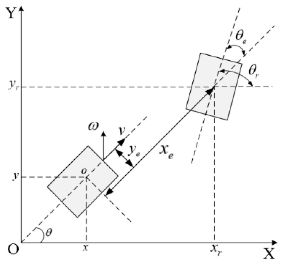
The schematic diagram of the pose error of the wheeled mobile robot is shown in Figure 3. Here, θ and θ r represent the angle between the actual heading of the vehicle and the positive direction of the X-axis and the given heading, respectively. The actual pose of the robot in the global coordinate system is denoted by x y θ T , the given pose is denoted by x r y r θ r T , and the deviation between the given pose and the actual pose is denoted by x e y e θ e T . Let v r and ω r represent the expected linear velocity and angular velocity of the robot during forward movement, respectively, and v and ω represent the actual linear velocity and angular velocity, respectively.
The expected pose expression given as follows:
x ˙ r y ˙ r θ ˙ r = cos θ r + σ sin θ r 0 sin θ r σ cos θ r 0 0 1 v r ω r
The trajectory tracking error of the wheeled mobile robot in the global coordinate system can be expressed as follows:
x e y e θ e = cos θ + σ sin θ sin θ σ cos θ 0 sin θ + σ cos θ cos θ + σ sin θ 0 0 0 1 x r x y r y θ r θ
Differentiating Equation (29) and combining it with Equation (28) yields the trajectory error model of the robot in a slipping state:
x ˙ e y ˙ e θ ˙ e = y e ω + ( 1 + σ 2 ) v r cos θ e ( 1 + σ 2 ) v x e ω + ( 1 + σ 2 ) v r sin θ e ω r ω
In this article, the main objective of trajectory tracking for wheeled mobile robots is as follows: in the slipping state, obtain an appropriate control input v ω T to make the trajectory tracking error x e y e θ e T of the robot bounded and satisfied lim t x e y e θ e T = 0 .

4.2. Design of Trajectory Tracking Controller Improved Rapid Variable Exponential Reaching Law and Its Performance Analysis Under Different Parameters

4.2.1. Improved Rapid Variable Exponential Reaching Law

In this paper, an improved rapid variable exponential reaching law proposed in reference [36] is used. This approach law introduces a variable index term on the basis of a rapid double exponential reaching law, and the specific equation is as follows:
s ˙ = k 1 s γ sgn ( s ) k 2 s b sgn ( s ) k 3 s
γ = a , s 1 1 , s < 1
where k 1 > 0 , k 2 > 0 , k 3 > 0 , a > 1,0 < b < 1 .
If s < 1 , the approximation law is s ˙ = k 1 s k 2 s b sgn ( s ) k 3 s , which is approximately equal to the rapid power approximation law. It not only ensures the reaching speed but also makes the system smoothly transition to the sliding mode stage, so as to effectively reduce chattering. If  s 1 , the approximation law is s ˙ = k 1 s a sgn ( s ) k 2 s b sgn ( s ) k 3 s , which has a faster convergence rate and can significantly reduce the convergence time.

4.2.2. Analysis of the Influence of Reaching Law Parameters on Performance

The impact of parameters in Equations (31) and (32) on the reaching law performance is analyzed as follows:
(1)
k 1 and exponent a: Govern the convergence speed in the large-error phase ( s 1 ). Increasing k 1 accelerates initial convergence, while a > 1 ensures high-power terms ( s a ) dominate far from the sliding surface, significantly improving initial convergence speed. Excessively large k 1 or a may exacerbate chattering.
(2)
k 2 and exponent b: Regulate dynamics near the sliding surface ( s < 1 ). Increasing k 2 shortens convergence time for small errors but may intensify chattering. Setting 0 < b < 1 enables fractional-power terms ( s b ) near the sliding surface, smoothing transitions and suppressing chattering.
(3)
k 3 : Ensures linear convergence and steady-state robustness against disturbances. Increasing k 3 accelerates overall convergence but may cause oscillations if oversized.
Optimization: An appropriate configuration of k 1 , k 2 , a , and b balances speed and smoothness, ensuring overshoot-free transient processes.

4.3. Design and Stability Analysis of Sliding Mode Trajectory Tracking Controller with Parameter Influence on Control Performance

4.3.1. Design of Trajectory Tracking Controller

From Equation (5), the following is obtained:
v ω = 1 s L 2 1 s R 2 ( 1 s L ) b 1 s R b ω L ω R
By conversion, the following expression is obtained:
ω L ω R = 1 r 1 1 s L b 2 ( 1 s L ) 1 1 s R b 2 ( 1 s R ) v ω
Substituting the estimated values of the slip ratio for the actual values yields the following:
ω L ω R = 1 r 1 1 s ^ L b 2 ( 1 s ^ L ) 1 1 s ^ R b 2 ( 1 s ^ R ) v ω
According to the time convergence characteristic of improved rapid variable exponential reaching law, the sliding surfaces are designed as follows:
s = s 4 s 5 = θ e n 1 x e n 2 ω r y e
where n 1 ,   n 2 > 0 , ω r 0 and is a constant.
The convergence dynamics of the sliding surfaces follow:
S ˙ = s ˙ 4 s ˙ 5 = = μ 11 s 4 μ 12 s 4 λ 1 sgn ( s 4 ) μ 13 s 4 B sgn ( s 4 ) μ 21 s 5 μ 22 s 5 λ 2 sgn ( s 5 ) μ 23 s 5 B sgn ( s 5 )
where λ = α , s < 1 s , s 1 , μ 11 , μ 12 , μ 21 , μ 22 , μ 13 , μ 23 >0, α > 1 , 0 < B < 1 .
Using Equations (33), (36) and (37), the trajectory tracking motion control law is derived as follows:
ω = ω r + μ 11 s 4 + μ 12 s 4 λ 1 sgn ( s 4 ) + μ 13 s 4 B sgn ( s 4 )
v = y e ω r 1 + σ 2 + v r 1 n 1 ( 1 + σ 2 ) n 2 ω r 2 x e μ 21 s 5 μ 22 s 5 λ 2 sgn ( s 5 ) μ 23 s 5 B sgn ( s 5 )
Substituting Equations (19), (38) and (39) into Equation (35) yields the angular velocities of the left and right wheels in the slip state.
Unlike existing studies that generally assume ideal adhesion conditions, this work explicitly considers the trajectory tracking problem under unknown slip conditions. By directly incorporating the output of the sliding mode observer into the control law, the controller achieves real-time disturbance compensation, ensuring robustness while significantly improving convergence speed.

4.3.2. Stability Analysis

Theorem 1.
Under the action of sliding mode tracking controllers (36) and (37) based on the improved rapid exponential reaching law, the trajectory tracking errors  x e y e , and  θ e  of the wheeled mobile robot can converge to 0 within a finite time.
Proof. 
(1) Proof that the sliding surface s 4 = θ e continuously approaches to 0 within a finite time:
Assuming the initial state of the system is s 0 = s i ( 0 ) > 1 , i = 1,2 , 3 , the convergence process of the system moving from its initial state to the sliding mode switching surface and converging to 0 can be divided into three stages. Stage 1: the system moves from its initial state to s i ( t 1 ) = 1 ; Stage 2: the system moves from s i ( t 1 ) = 1 to s i ( t 2 ) = B ; Stage 3: the system moves from s i ( t 2 ) = B to s i ( t 3 ) = 0 .
Stage 1: When the system moves from the initial state s 0 = s i ( 0 ) > 1 to s i ( t 1 ) = 1 , it is known that s 4 > 1 . During this phase, the reaching law simplifies to the following:
s ˙ 4 = μ 11 s 4 μ 12 s 4 a μ 13 s 4 B
From Equation (40), it can be seen that there are two power-law equations. These can be decomposed into s ˙ 4 + μ 11 s 4 = μ 12 s 4 a and s ˙ 4 + μ 11 s 4 = μ 13 s 4 B , which are solved separately. s ˙ 4 + μ 11 s 4 = μ 12 s 4 a denotes the required approach time when the system is influenced only by μ 12 s a sgn ( s ) , and s ˙ 4 + μ 11 s 4 = μ 13 s 4 B denotes the required approach time when influenced only by μ 13 s B sgn ( s ) . Therefore, the approach time of Equation (41) must be less than either of the above solutions:
To solve s ˙ 4 + μ 11 s 4 = μ 12 s 4 a , the process is as follows:
s 4 a d s 4 d t + μ 11 s 4 1 a = μ 12
Assuming the existence of an intermediate variable A = s 4 1 a , Equation (41) can be written as follows:
d A d t + 1 a μ 11 A = 1 a μ 12
Solving Equation (42) gives the following:
A = ( 1 a ) μ 12 e ( 1 a ) μ 11 d t d t + C 1 e ( 1 a ) μ 11 d t = C 1 e ( 1 a ) μ 11 d t μ 12 e ( 1 a ) k 3 d t k 3 e ( 1 a ) μ 11 d t = C 1 e ( 1 a ) μ 11 t μ 12 μ 11
Namely:
s 4 1 a = C 1 e ( 1 a ) μ 11 t μ 12 μ 11
When t = 0 , s i ( 0 ) = s 0 , the constant C 1 can be solved:
C 1 = s 0 1 a μ 12 μ 11
The solution to Equation (41) is obtained using Expressions (44) and (45):
t 1 = 1 ( 1 a ) μ 11 ln ( s 4 1 a + μ 12 μ 11 ) ln ( s 0 1 a + μ 12 μ 11 )
So the time required to move from s 0 to s i ( t 1 ) = 1 is as follows:
T 1 = 1 ( 1 a ) μ 11 ln ( a 1 a + μ 12 μ 11 ) ln ( s 0 1 a + μ 12 μ 11 )
Therefore, the time required for the system to move from    s 0 to s i ( t 1 ) = 1 is less than T 1 , that is, the actual convergence time of s 4 = θ e in the first stage is less than T 1 .
Stage 2: The system moves from s i ( t 1 ) = 1 to s i ( t 2 ) = B . In this case, the approximation law can still be expressed by Equation (40).
To solve s ˙ 4 + μ 11 s = μ 13 s B , similarly, it can be solved that:
s 4 1 B = C 2 e ( 1 B ) μ 11 t μ 13 μ 11
When t = 0 , s 4 = 1 , then C 2 = 1 + μ 13 μ 11 , then corresponding time can be calculated as follows:
t 2 = 1 ( B 1 ) μ 11 ln ( s 4 1 B + μ 13 μ 11 ) ln ( 1 + μ 13 μ 11 )
So the time required f to move from s i ( t 1 ) = 1 to s i ( t 2 ) = B is as follows:
T 2 = 1 ( B 1 ) μ 11 ln ( B 1 B + μ 13 μ 11 ) ln ( 1 + μ 13 μ 11 )
Therefore, the time required for the system to move from s i ( t 1 ) = 1 to s i ( t 2 ) = B is less than T 2 , that is, the actual convergence time of s 4 = θ e in the second stage is less than T 2 .
Stage 3: The system moves from s i ( t 2 ) = B to s i ( t 3 ) = 0 , and it can be inferred that s 4 < 1 . At this point, the law of approximation can be written as follows:
s ˙ 4 = μ 12 s 4 μ 13 s 4 B μ 11 s 4 = ( μ 11 + μ 12 ) s μ 13 s B
Similarly:
t 3 = 1 ( B 1 ) ( μ 11 + μ 12 ) ln ( s 4 1 B + μ 13 μ 11 + μ 12 sgn ( s 0 ) ) ln ( B 1 B + μ 13 μ 11 + μ 12 sgn ( s 0 ) )
Namely, the time required for the system to move s i ( t 2 ) = B to s i ( t 3 ) = 0 is as follows:
T 3 = 1 ( B 1 ) ( μ 11 + μ 12 ) ln ( 1 + μ 13 μ 11 + μ 12 sgn ( s 0 ) ) ln ( B 1 B + μ 13 μ 11 + μ 12 sgn ( s 0 ) )
In summary, when the initial state s 0 > 0 , the time for the system to reach the sliding mode surface from its initial state and converge to 0 should be less than the sum of the time required for the above three stages T 1 + T 2 + T 3 .
When the initial state s 0 < 0 , the time for the system to reach the sliding mode sur face from its initial state and converge to 0 can also be divided into three stages. The solution principle is the same as for the system with initial state s 0 > 0 mentioned above.
(2) Prove that the sliding mode surface s 5 = n 1 x e n 2 ω r y e converges to 0 within a finite time.
Let the convergence times of s 4 and s 5 be t s 4 and t s 5 respectively. Therefore, when the total time t > t s 4 + t s 5 , the sliding surfaces s 4 and s 5 can converge to 0, and the angular velocity and linear velocity are as follows:
ω = ω r
v = y e ω r + v r + n 2 ω r 2 x e n 1
In this case, Equation (30) can be rewritten as follows:
x ˙ e = y e ω r + v r v
y ˙ e = x e ω
Assuming that the Lyapunov function is V x = 1 2 x e 2 , its derivative can be obtained as follows:
V ˙ x = x e x ˙ e = x e ( y e ω r + v r v ) = x e ( y e ω r + v r y e ω r v r n 2 ω r 2 x e n 1 ) = n 2 ω r 2 x e 2 n 1 = 2 n 2 ω r 2 V x n 1 0
So when ω r 0 , x e will converge asymptotically to 0, at this time: y e = n 1 x e s 2 n 2 ω r .
Since x e , s 4 , and s 5 can converge asymptotically to 0, it can be inferred that y e will also converge asymptotically to 0.
In summary, under the influence of trajectory tracking controller based on the improved exponential reaching law, x e , y e , and θ e can all converge to 0 in a finite time. □

4.3.3. Analysis of the Influence of Sliding Mode Trajectory Tracking Controller Parameters on Control Performance

(1)
μ 11 / μ 21 (Linear term coefficients): Directly determine the exponential convergence rate of errors. Increasing them accelerates linear error convergence but may induce overshoot and oscillations.
(2)
μ 12 / μ 22 (High-power term coefficients): Dominate rapid convergence in the large-error phase ( | s | 1 ).
(3)
μ 13 / μ 23 (Fractional-power terms): Optimize smoothness in the small-error phase ( s < 1 ), avoiding steady-state chattering.
(4)
n 1 / n 2 ratio: Determines the convergence speed of position error x e via Equation (58). Increasing the ratio accelerates x e convergence but may cause oscillations (e.g., oversized n 1 or undersized n 2 in simulations). The optimal ratio balances speed and smoothness. Simulations use n 1 = 16.4, n 2 = 17.8 (ratio ≈ 0.92) to ensure convergence while suppressing oscillations.

5. Simulation and Experiment

5.1. Simulation Verification

To verify the effectiveness of the trajectory tracking controller designed in this paper, a simulation study is conducted using MATLAB R2023a software for the trajectory tracking control problem of wheeled mobile robots. The desired linear velocity and angular velocity are selected as v r = 1.8 m / s and ω r = 1.2   r a d / s , respectively. The desired initial pose of the robot is set to 3 1 1 T , and the actual initial pose is 2 1 2 T .
From Equation (37), it can be seen that the convergence speed of the sliding mode surface is influenced by parameters λ 1 and λ 2 . Through simulation experiments to adjust λ 1 and λ 2 , it was found that when λ 1 > 0.5 and λ 2 > 4 , the system will exhibit significant oscillations.Furthermore, from expressions (47), (50), and (53), it can be seen that the approach time of the system is influenced by parameters μ 11 , μ 12 , μ 13 , μ 21 , μ 22 , and μ 23 ; therefore, the convergence time of the system can be controlled by adjusting the values of these parameters. From Equation (58), it can be seen that the convergence speed of x e is determined by the ratio of n 2 / n 1 . In simulations, by adjusting the values of n 1 and n 2 , it is not difficult to observe that when the value of n 1 is too large or the value of n 2 is too small, the system will exhibit excessive oscillations.
In summary, various parameters were adjusted based on the simulation results, and the final selection was μ 11 = 6 , μ 12 = 2 , μ 13 = 1 , μ 21 = 7 , μ 22 = 3 , μ 23 = 2 , λ 1 = 0.2 , λ 2 = 3 , B = 1.5, n 1 = 16.4 ,   a n d   n 2 = 17.8 . According to Equations (26) and (27), the sliding mode gains are determined as L 3 = 2 r ω L / b , L 4 = 2 r ω R / b , and the initial values for sliding parameter estimation are set to s L ( 0 ) = s R ( 0 ) = 0 . During the robot’s movement, the actual slip parameters of the left and right wheels at the 20th second are assumed to be s L = 0.4 and s R = 0.4 , respectively, with perturbations of amplitude 0.05 introduced from the 32nd to the 35th second:
(1)
The tracking path of the robot is selected as a circular shape, and its reference trajectory is as follows:
x r ( t ) = cos ( ω r t ) y r ( t ) = sin ( ω r t ) θ r = ω r t
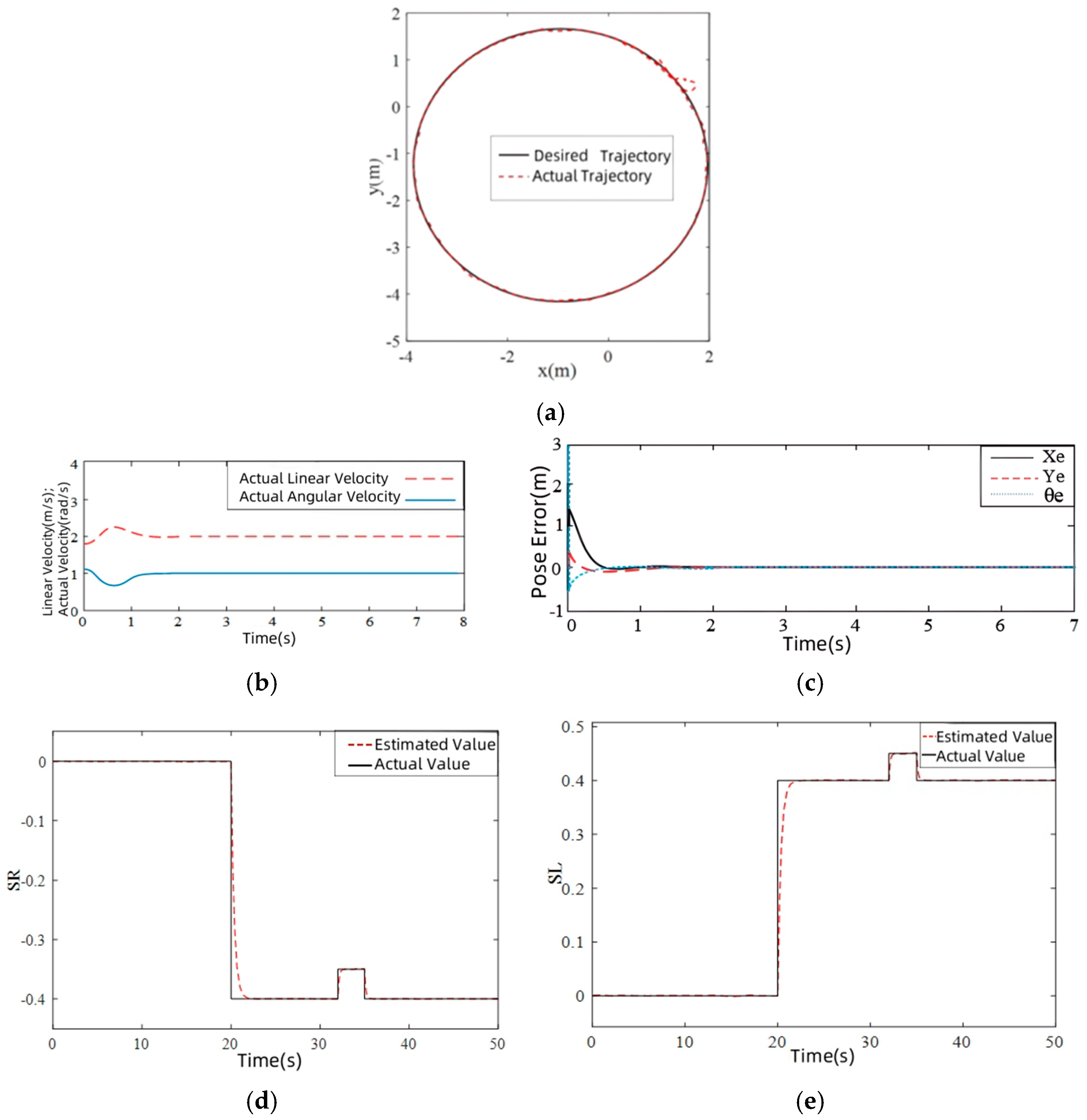
The simulation results are shown in Figure 4, and Table 1 presents the dynamic performance indicators for tracking the circular trajectory under the influence of slip ratio.
From Figure 4 and Table 1, it can be observed that the robot’s pose errors x e , y e , and θ e converge to 0 within 0.66 s, 0.51 s, and 0.76 s, respectively. This means that the robot fully tracks the desired circular trajectory after 0.76 s. The robot’s linear velocity and angular velocity converge to the desired values within 1.37 s and 1.24 s, respectively. And after only one oscillation, the steady state is reached, which indicates that the whole tracking process runs smoothly and is hardly affected by the slip rate. As shown in Figure 4d,e, the sliding mode observer can accurately predict the slip ratio, which is the foundation for good trajectory tracking performance.
(2)
The tracking path of the robot is selected as “8” shape, and its reference trajectory is as follows:
x r ( t ) = 30 sin ( t 10 ) y r ( t ) = 30 sin ( t 20 )
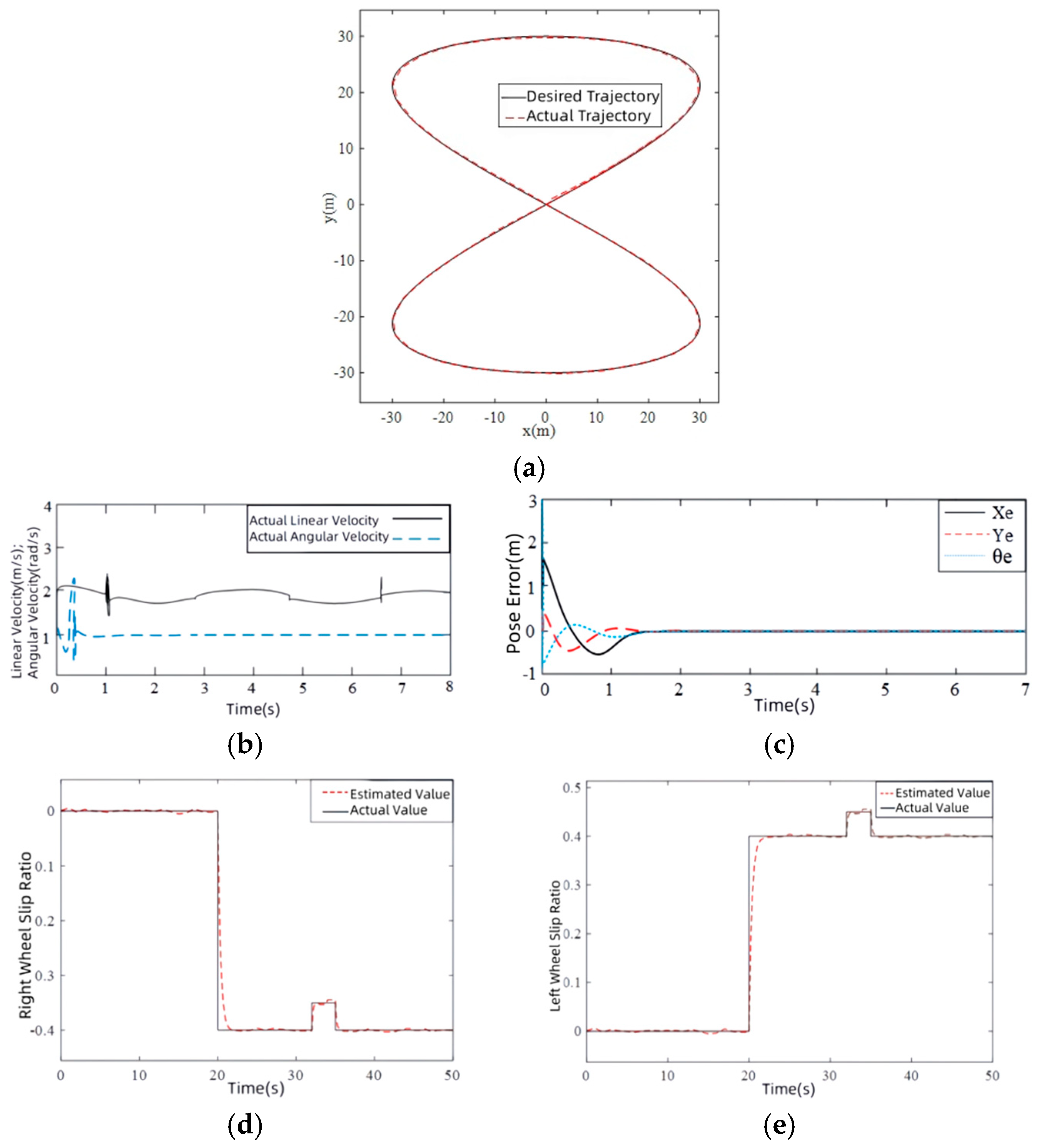
The simulation results are shown in Figure 5, and Table 2 presents dynamic performance indicators for tracking the “8”-shaped trajectory under the influence of slip ratio.
Due to the greater difficulty in tracking the “8”-shaped trajectory, it can be seen from Figure 5 and Table 2 that the convergence times of the robot’s pose error, linear velocity, and angular velocity are longer, and the number of oscillations during the transition process and the overshoots of various variables have also increased. However, after 1.48 s, it fully tracked the desired “8”-shaped trajectory. Similarly, the sliding mode observer also accurately estimated the slip rates of the left and right wheels.
(3)
The tracking path of the robot is selected as a sinusoidal shape, with its reference trajectory being the following:
x r ( t ) = t y r ( t ) = sin t θ r ( t ) = ω r t
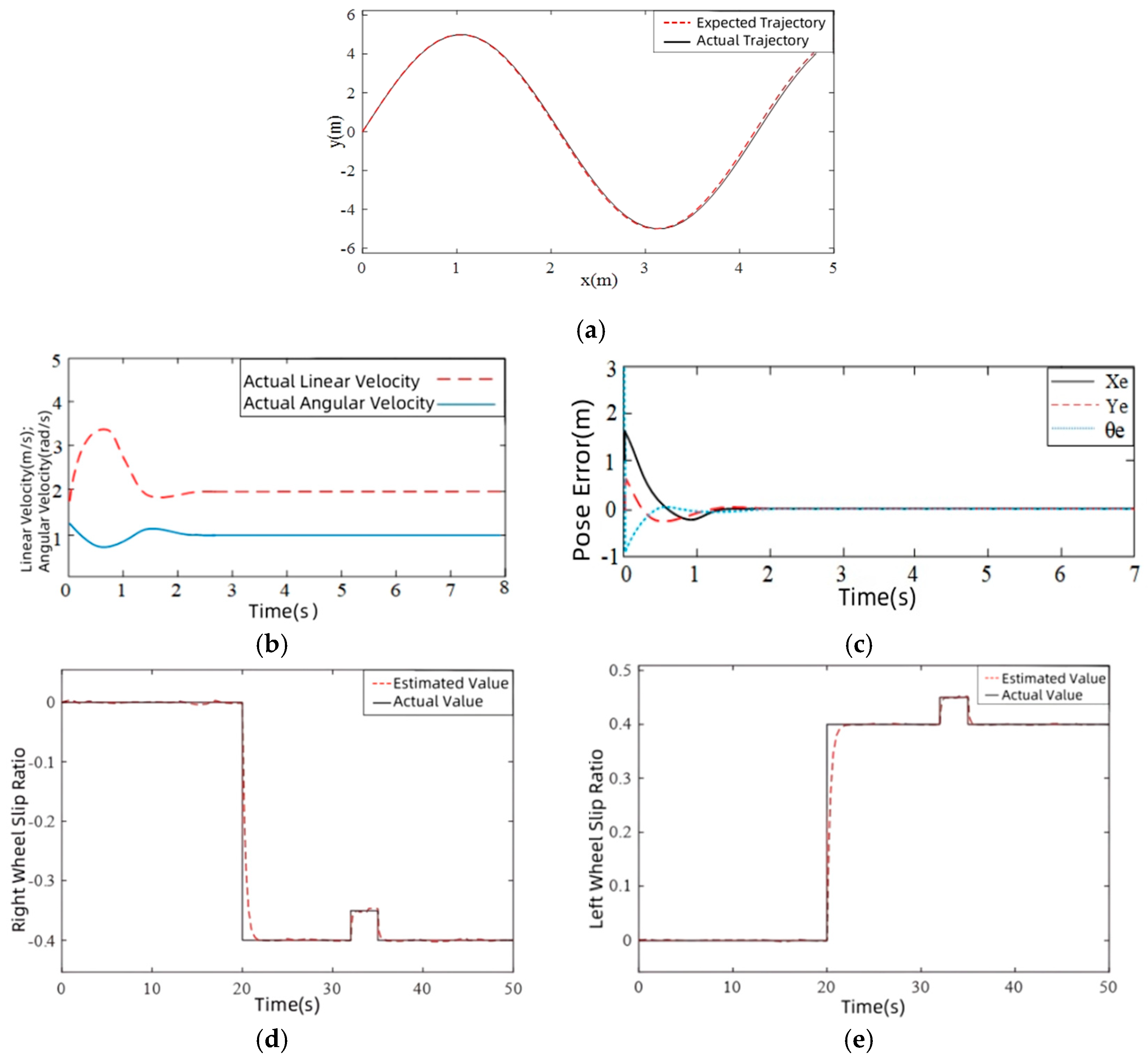
The simulation results are shown in Figure 6, and Table 3 presents the dynamic performance indicators for tracking the sinusoidal shape trajectory under the influence of slip ratio.
Due to the higher frequency of changes in the sinusoidal trajectory compared to the “8”-shaped trajectory, the tracking difficulty is greater. As can be seen from Figure 6 and Table 3, the robot’s pose error, linear velocity, and angular velocity converge over a longer period of time. However, after 1.56 s, it fully tracked the desired sinusoidal trajectory, and after 2.12 s, both linear velocity and angular velocity reached the desired values. The sliding mode observer also estimated the slip rates of the left and right wheels in a timely manner.
Based on the above simulation results, it can be concluded that the trajectory tracking controller designed in this paper achieves good tracking performance when tracking circular, “8”-shaped, and sinusoidal trajectories. As can be seen from sub-figures (a) and (c) of Figure 4, Figure 5 and Figure 6, the actual trajectories of the robot are very close to the desired trajectories, and as time goes by, the error between the two gradually decreases and approaches 0, indicating that the controller has strong tracking and convergence performance. Even if the sliding parameters change, the designed sliding mode observer can still accurately estimate, further verifying the effectiveness of the sliding mode observer and the robustness of the trajectory tracking controller designed in this paper.

5.2. Simulation Comparison Verification

To verify the control effect of the trajectory tracking controller with the sliding mode observer designed in this paper, a set of simulation comparison experiments was conducted using circular trajectory tracking as an example (with experimental conditions identical to those in Section 4.1). The experimental contents include the following:
(1)
Replace the convergence law of the sliding mode trajectory tracking controller designed in Section 3.2 with a rapid double exponential reaching law, keeping other aspects unchanged. The result of tracking the circular trajectory is shown in Figure 7.
(2)
Let the slip rate parameters S ^ L and S ^ R in Equation (35) be 0; the sliding mode observer is not used to estimate the slip rate, nor is the influence of the slip rate considered in the control; the others remain unchanged. The result of tracking the circular trajectory is shown in Figure 8.
(3)
Due to the ability of fuzzy PID controller to adjust PID parameters in real time according to environmental changes, it has strong environmental adaptability and robustness. Therefore, in this section, the fuzzy PID control algorithm was used to design a trajectory tracking controller. Other experimental conditions remain unchanged; the result of tracking the circular trajectory is shown in Figure 9.
The comparison results of the adjustment times of robot pose error and tracking speed are shown in Table 4.
Comparing Figure 4a, Figure 7, Figure 8, Figure 9 and Table 4, it can be seen that the trajectory tracking controller designed using the fuzzy PID control algorithm has the worst tracking effect. The trajectory tracking controller based on the improved rapid variable exponential reaching law with the sliding mode observer designed in this paper has the best tracking effect. This is due to two factors. Firstly, although fuzzy PID control can adjust PID parameters in real time according to environmental changes, it cannot effectively identify and cancel out unknown slip ratio disturbances solely based on fuzzy rules. Secondly, fuzzy PID control needs to adjust parameters through multiple iterations and rule matching, which limits the real-time performance of the system to a certain extent. The trajectory tracking controller designed in this article can accurately estimate the slip parameters using the sliding mode observer and introduce the observation results into the trajectory tracking controller for control, which can quickly eliminate the influence of slip rate. On the other hand, the improved rapid variable exponential reaching law possesses faster reaching speed and can effectively reduce chattering, so the trajectory tracking process is stable and smooth.
From Table 4, it can be seen that compared to the other three control schemes, the trajectory tracking controller designed in this paper significantly reduces convergence times of the tracking errors ( x e , y e , θ e ), linear velocity v , and angular velocity ω . The convergence times of the above variables are only 25.19%, 20.56%, 24.92%, 34.42%, and 32.98% of that of the fuzzy PID trajectory tracking controller, respectively, and the convergence times of the above variables are only 65.34%, 64.56%, 80.85%, 61.43%, and 61.68% of that of the fast double power law trajectory tracking controller with sliding mode observer, which has better relative control effect compared to the other two control schemes.
While the reaching law employed in the trajectory tracking controller (Figure 7) demonstrates relatively weaker performance compared to Figure 8, the system still achieves superior tracking performance to controllers using the improved rapid variable exponential reaching law without slip ratio compensation. This enhancement stems from two key factors: (1) the sliding mode observer’s effective slip ratio estimation, and (2) the controller’s explicit consideration of slip effects. Although minor trajectory fluctuations and deviations persist (Figure 8), these results conclusively demonstrate the necessity of incorporating a sliding mode observer to estimate slip rates and feed this critical information into the control system.

5.3. Experimental Verification

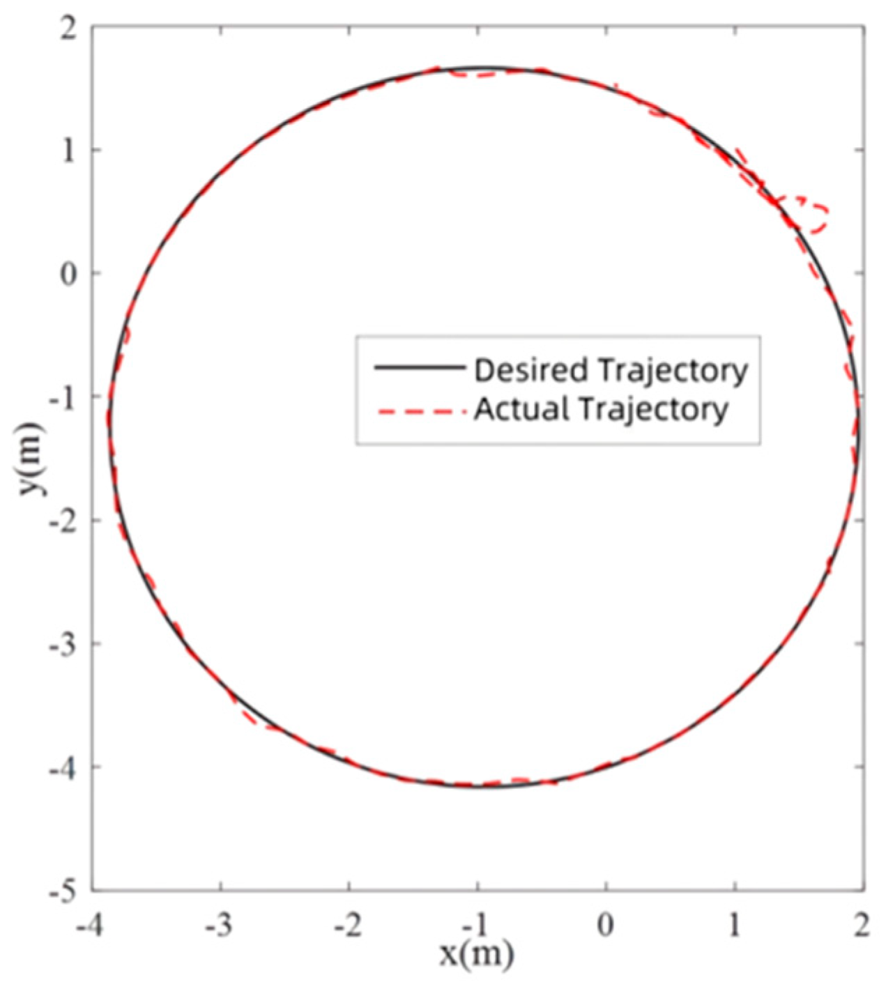
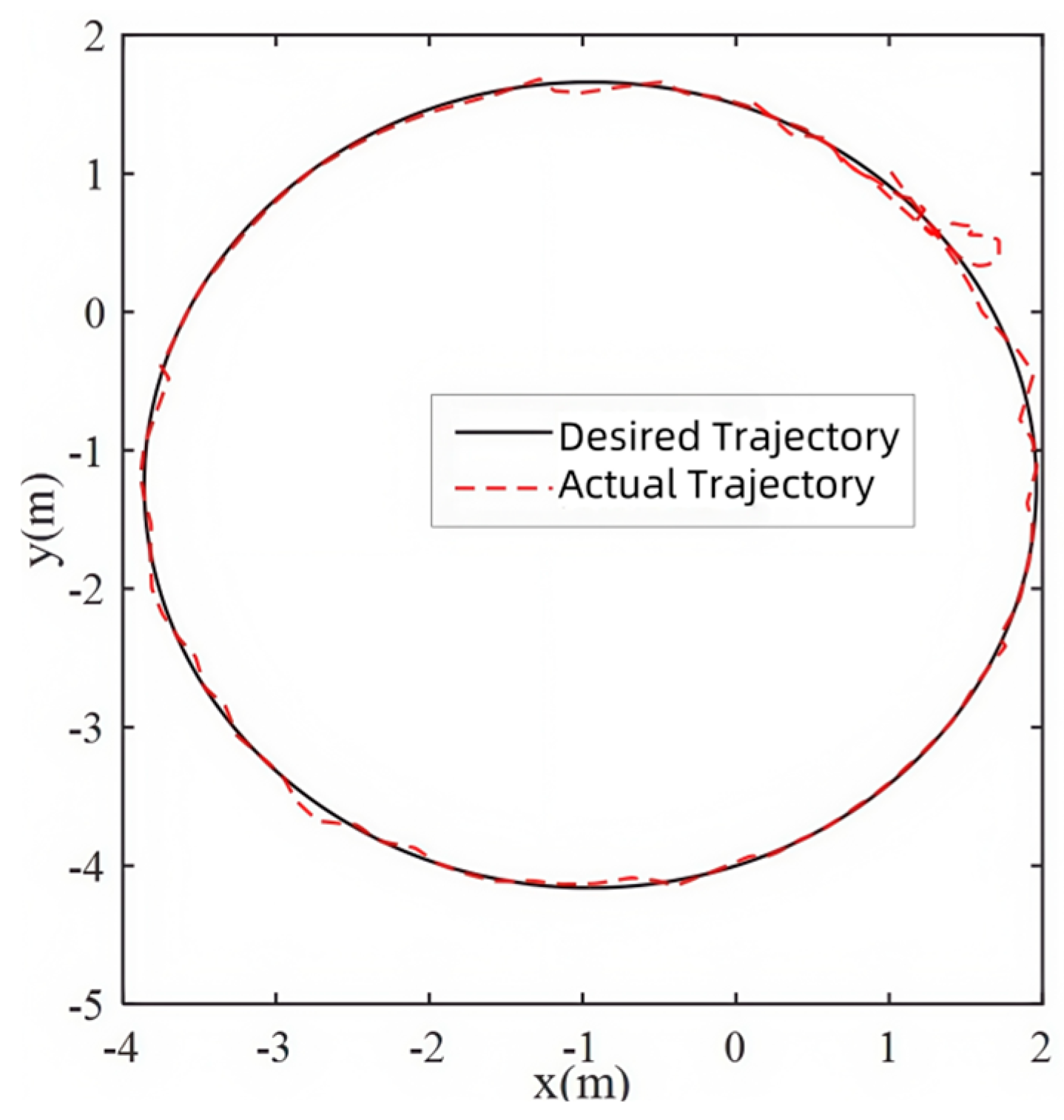
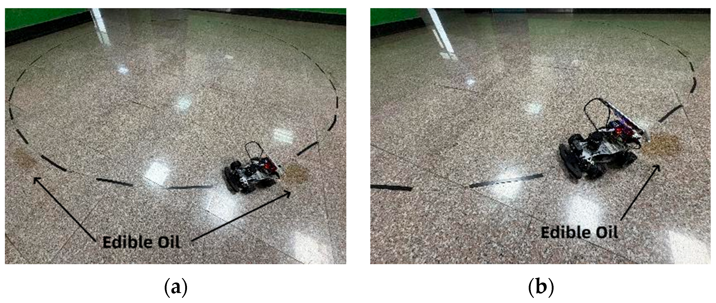
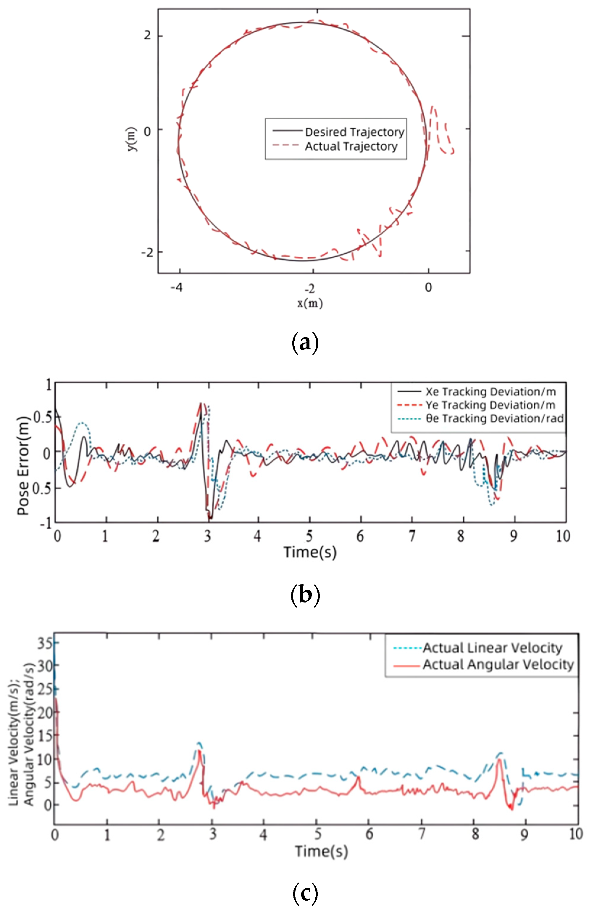
To validate the effectiveness of the trajectory tracking controller designed in this paper in the actual environment, experiments were conducted using a wheeled mobile robot. The physical parameters of the robot are as follows: overall mass m = 3 kg, distance between front and rear wheels l = 0.2 m, and the distance from the center point to the side of the wheel d = 0.1 m. Edible oil was poured on the ground to make the wheels slip, as shown in Figure 10, where the radius of the circular trajectory is 2 m, and the dashed line represents the given motion trajectory for the robot. The specific experimental results are shown in Figure 11.
From Figure 11, it can be seen that the oil on the ground causes the wheel to slip. At the moment when the oil is stained, the trajectory tracking error range becomes larger, the speed fluctuation is intensified, and the convergence performance becomes worse. This is because in the actual operation, the tracking error will be further increased by the moment of inertia, damping effect of the left and right wheel motors, and the driving force attenuation caused by the slip due to the ground slip. As illustrated in Figure 11b,c, at t = 2.5 s, the error suddenly increases due to slipping, and the wheel torque required to maintain the robot’s turning will also increase. Although the sliding mode observer can correct the slip parameters in real time, the motor torque saturation characteristics still cause short-term control lag. Afterwards, within approximately 1 s, the torque demand is restricted within the motor’s feasible range, thereby restoring tracking.
In addition, the rapid double exponential reaching law is used to verify the trajectory tracking effect in the actual environment under the same experimental conditions, and the specific results are shown in Figure 12.
From the comparison of Figure 11 and Figure 12, it can be observed that under the same conditions, the trajectory tracking controller designed in this paper has better tracking performance.

6. Limitations and Future Work

Although the proposed control method demonstrates high robustness and accuracy under unknown slip conditions, several limitations remain. First, the experimental validation primarily focuses on scenarios with constant slip rates or single abrupt slip changes, without fully addressing the complex dynamics during high-speed cornering or large velocity variations. Second, the adaptability of the controller to a wide range of road surfaces (e.g., wet, gravel) has not been systematically tested. In addition, the tuning of controller parameters still relies on offline adjustment, lacking a fully adaptive online optimization mechanism.
Future work will focus on the following: (1) verifying and optimizing the robustness of the control strategy in more complex dynamic scenarios such as high-speed turns and sudden acceleration/deceleration; (2) improving the accuracy and real-time performance of slip rate estimation through multi-sensor fusion; (3) introducing an online parameter adaptation mechanism to reduce dependency on manual tuning; and (4) extending applicability tests to various road surface types and weather conditions.

7. Conclusions

This study proposes a trajectory tracking control scheme incorporating a slip ratio observer. The proposed control framework consists of three core components: (1) a sliding mode observer for real-time estimation of unknown slip ratios; (2) an improved rapid variable-power reaching law that accelerates convergence and mitigates chattering; and (3) an integrated control structure that directly incorporates the observer’s output into the control law. Theoretical analysis proves the stability and finite-time convergence of the system. Compared with traditional methods, this study deeply couples the sliding mode observer with the improved rapid variable-power reaching law within a unified framework, achieving adaptive parameter adjustment and disturbance compensation, thereby maintaining high-precision trajectory tracking performance even under sideslip conditions. Simulation and experimental results show that the proposed control scheme not only achieves high-accuracy and smooth trajectory tracking under unknown slip conditions but also significantly enhances convergence speed, reducing the shortest convergence time to only 20.56% of that of an environmentally adaptive fuzzy PID trajectory tracking controller and 61.43% of that of a rapid double-power reaching law controller with a sliding mode observer.
The findings of this study are of considerable importance from both theoretical and practical perspectives. Theoretically, the proposed control strategy effectively addresses the challenges faced by wheeled mobile robots under slip conditions, delivering more accurate and robust trajectory tracking performance compared with conventional methods. Practically, the successful validation through both simulations and real-world experiments demonstrates the applicability of the method in complex operating environments. Such robustness and adaptability are particularly valuable for tasks requiring high precision and reliability, such as autonomous navigation, industrial logistics, and field robotics. These results not only confirm the feasibility of the proposed approach but also lay a solid foundation for its integration into broader intelligent robotic systems, where safety, accuracy, and adaptability are of paramount importance.

Author Contributions

Conceptualization, Z.L.; data curation, X.X.; funding acquisition, X.L.; investigation, T.W.; methodology, Z.L.; resources, Y.F.; software, J.G.; supervision, X.X.; validation, J.G.; visualization, Z.L.; writing—original draft, Z.L.; writing—review & editing, X.L. All authors have read and agreed to the published version of the manuscript.

Funding

This work was supported by the National Natural Science Foundation of China [Grant No. 317972209] and the Key Research and Development Projects of Shaanxi Province, China [Grant No. 2021NY-059].

Institutional Review Board Statement

The work contains no defamatory or illegal content, violates no third-party rights, and includes no hazardous materials or procedures that could result in harm.

Data Availability Statement

The original contributions presented in this study are included in the article. Further inquiries can be directed to the corresponding author.

Conflicts of Interest

Author Yong Feng was employed by the company Filtang Technologies Corporation, Yantai 264006, China. The remaining authors declare that the research was conducted in the absence of any commercial or financial relationships that could be construed as a potential conflict of interest.

References

  1. Li, B.; Wang, C.H.; Ma, L.; Zhang, H.C. Fixed-time trajectory tracking control for a wheel mobile robot. Control Decis. 2024, 39, 845–852. [Google Scholar]
  2. Xu, S.; Ou, Y.S.; Wang, Z.Y.; Li, H. Learning-based kinematic control using position and velocity errors for robot trajectory tracking. IEEE Trans. Syst. Man Cybern. Syst. 2022, 52, 1100–1110. [Google Scholar] [CrossRef]
  3. Kim, Y.; Singh, T. Energy-time optimal trajectory tracking control of wheeled mobile robots. IEEE/ASME Trans. Mechatron. 2024, 29, 1283–1294. [Google Scholar] [CrossRef]
  4. Liu, X.; Wang, W.; Li, X.; Liu, F.; He, Z.; Yao, Y.; Ruan, H.; Zhang, T. MPC-based high-speed trajectory tracking for 4WIS robot. ISA Trans. 2022, 123, 413–424. [Google Scholar] [CrossRef]
  5. Wang, S.; Li, G.; Song, J.; Liu, B. Research on an intelligent vehicle trajectory tracking method based on optimal control theory. World Electr. Veh. J. 2024, 15, 160. [Google Scholar] [CrossRef]
  6. Wu, H.; Wang, S.; Xie, Y.; Li, H.; Zheng, S.; Jiang, L. Adaptive abrupt disturbance rejection tracking control for wheeled mobile robots. IEEE Robot. Autom. Lett. 2024, 9, 7787–7794. [Google Scholar] [CrossRef]
  7. Li, H.; Bi, L.Z.; Yi, J. Sliding-mode nonlinear predictive control of brain-controlled mobile robots. IEEE Trans. Cybern. 2022, 52, 5419–5431. [Google Scholar] [CrossRef] [PubMed]
  8. Ryoo, Y.J. Trajectory-tracking control of a transport robot for smart logistics using the fuzzy controller. Int. J. Fuzzy Log. Intell. Syst. 2022, 22, 69–77. [Google Scholar] [CrossRef]
  9. Dong, C.; Yu, Z.; Chen, X.; Huang, Y.; Huang, Q. Adaptability control towards complex ground based on fuzzy logic for humanoid robots. IEEE Trans. Fuzzy Syst. 2022, 30, 1574–1584. [Google Scholar] [CrossRef]
  10. Falsafi, M.H.; Alipour, K.; Tarvirdizadeh, B. Tracking-error fuzzy-based control for nonholonomic wheeled robots. Arab. J. Sci. Eng. 2019, 44, 881–892. [Google Scholar] [CrossRef]
  11. Tan, W.; Wang, M.; Ma, K. Research on intelligent vehicle trajectory tracking control based on improved adaptive MPC. Sensors 2024, 24, 2316. [Google Scholar] [CrossRef] [PubMed]
  12. Chen, Y.J.; Zhao, F.H.; Lou, Y.J. Interactive model predictive control for robot navigation in dense crowds. IEEE Trans. Syst. Man Cybern. Syst. 2022, 52, 2289–2301. [Google Scholar] [CrossRef]
  13. Gao, Y.; Wang, X.; Huang, J.; Yuan, L. Adaptive model predictive control for intelligent vehicle trajectory tracking considering road curvature. Int. J. Automot. Technol. 2024, 25, 1051–1064. [Google Scholar] [CrossRef]
  14. Yang, H.; Wang, J.; Li, S.; Chen, W. Trajectory tracking for wheeled mobile robots via model predictive control with softening constraints. IET Control Theory Appl. 2018, 12, 206–214. [Google Scholar] [CrossRef]
  15. Silaa, M.Y.; Bencherif, A.; Barambones, O. Indirect adaptive control using neural network and discrete extended Kalman filter for wheeled mobile robot. Actuators 2024, 13, 51. [Google Scholar] [CrossRef]
  16. Lu, X.; Fei, J. Velocity tracking control of wheeled mobile robots by iterative learning control. Int. J. Adv. Robot. Syst. 2016, 13, 103. [Google Scholar] [CrossRef]
  17. Hassan, N.; Saleem, A. Neural network-based adaptive controller for trajectory tracking of wheeled mobile robots. IEEE Access 2022, 10, 13582–13597. [Google Scholar] [CrossRef]
  18. Wu, X.; Li, X.; Zhang, D.; Wang, Y.; Zhang, Q. A control strategy for point stabilization and trajectory tracking of wheeled mobile robots. Robot. Auton. Syst. 2025, 173, 105040. [Google Scholar] [CrossRef]
  19. Kang, Z.; Zhang, H.; Huang, K.; Zhao, H.; Zhang, Y. Adaptive trajectory tracking of wheeled mobile robots based on a fish-eye camera. Int. J. Control Autom. Syst. 2019, 17, 2297–2309. [Google Scholar] [CrossRef]
  20. Zhang, K.; Chai, B.; Tan, M. Optimal enhanced backstep method for trajectory tracking control of the wheeled mobile robot. Optim. Control Appl. Methods 2024, 45, 2762–2790. [Google Scholar] [CrossRef]
  21. Binh, N.T.; Tung, N.A.; Nam, D.P.; Quang, N.H. An adaptive backstep trajectory tracking control of a tractor trailer wheeled mobile robot. Int. J. Control Autom. Syst. 2019, 17, 465–473. [Google Scholar] [CrossRef]
  22. Villalobos-Aranda, C.; Pliego-Jiménez, J.; Montañez-Molina, C.; Arellano-Delgado, A. An almost global trajectory tracking controller for differential-drive wheeled mobile robots. Int. J. Control Autom. Syst. 2024, 22, 3684–3693. [Google Scholar] [CrossRef]
  23. Petrov, P.; Kralov, I. Exponential trajectory tracking control of nonholonomic wheeled mobile robots. Mathematics 2024, 13, 1. [Google Scholar] [CrossRef]
  24. Yuan, L.; Li, J.N. Consensus of discrete-time nonlinear multiagent systems using sliding mode control based on optimal control. IEEE Access 2022, 10, 47275–47283. [Google Scholar] [CrossRef]
  25. Sharma, A.K.; Bhushan, B. Comparison of various fuzzy sliding mode based controller on single link inverted pendulum. J. Intell. Fuzzy Syst. 2022, 42, 679–688. [Google Scholar] [CrossRef]
  26. Lin, H.Z.; Li, Y.M.; Yuan, Z.H.; Wu, T.; Liu, C.L. Sliding mode anti-interference path tracking method for autonomous operation of paddy field plant protection machine. Trans. Chin. Soc. Agric. Mach. 2021, 52, 383–388. [Google Scholar]
  27. Wang, Z.; Pang, A.M.; Ma, S.B. Novel sliding mode control of mobile robot based on differential evolution algorithm. Modul. Mach. Tool Autom. Manuf. Tech. 2022, 9, 72–75+79. [Google Scholar]
  28. Geng, Z.W.; Wang, S.; Yang, S.Y. Tracking control of wheeled mobile robot based on backstepping and hierarchical sliding mode control. Manuf. Autom. 2022, 44, 109–112. [Google Scholar]
  29. Wang, L.L.; Dong, L.Y.; Ma, D.; Liu, X.L.; Wang, H.R. Active disturbance rejection tracking control of wheeled mobile robots under sliding and slipping conditions. Control Theory Appl. 2020, 37, 431–438. [Google Scholar]
  30. Li, Z.Y.; Dong, F.M.; Dian, S.Y.; Zhao, T. Anti-windup fuzzy super-twisting sliding mode control of WMRs with skidding and slipping. Comput. Simul. 2022, 39, 387–393+398. [Google Scholar]
  31. Jia, S.M.; Lu, X.Y.; Zhang, X.Y.; Zhang, G.L. Trajectory tracking control for omnidirectional mobile robot in presence of wheel slipping. Control Decis. 2020, 35, 833–842. [Google Scholar]
  32. Han, X.; Ge, M.; Cui, J.; Wang, H.; Zhuang, W. Motion modeling of a non-holonomic wheeled mobile robot based on trajectory tracking control. Trans. Can. Soc. Mech. Eng. 2020, 44, 228–233. [Google Scholar] [CrossRef]
  33. Yang, X. Research on Key Technology of Multi-Mode Motion Control for Reconfigurable Mobile Robot. Ph.D. Thesis, Chongqing University, Chongqing, China, 2023. [Google Scholar]
  34. Bai, H.; Song, X.G.; Ding, L.; Xia, K.R.; Li, N.; Deng, Z.Q. Adaptive motion control of wheeled mobile robot with unknown slippage. Int. J. Control 2014, 87, 1513–1522. [Google Scholar]
  35. Sergiyenko, O.; Tyrsa, V.; Zhirabok, A.; Zuev, A. Sensor fault identification in linear and nonlinear dynamic systems via sliding mode observers. IEEE Sens. J. 2022, 22, 10173–10182. [Google Scholar] [CrossRef]
  36. Li, Y.; Sun, R.; Xia, Y.; Gu, C. A sliding mode control method with improved rapid power approximation law. J. Xi’an Jiaotong Univ. 2022, 56, 118–126. [Google Scholar]
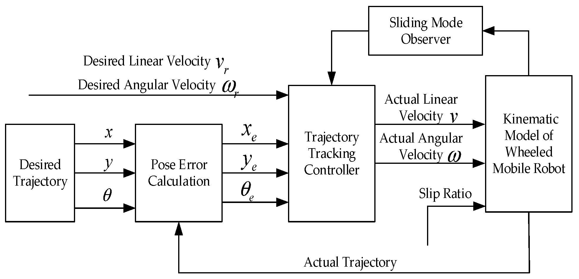
Figure 1. Control block diagram.
Machines 13 00765 g001
Figure 2. Schematic diagram of wheeled robot movement in slipping state.
Machines 13 00765 g002
Figure 3. Schematic diagram of pose error of wheeled mobile robot.
Machines 13 00765 g003
Figure 4. Simulation results of circular trajectory tracking. (a) Circular trajectory tracking curves. (b) Trajectory tracking linear velocity and angular velocity curves. (c) Trajectory tracking pose error curves of robots. (d) Right wheel slip rate estimation curves. (e) Left wheel slip rate estimation curves.
Machines 13 00765 g004
Figure 5. Simulation results of “8”-shaped trajectory tracking. (a) “8”-shaped trajectory tracking curve. (b) Trajectory tracking linear velocity and angular velocity curves. (c) Trajectory tracking pose error curves of robots. (d) Right wheel slip rate estimation curves. (e) Left wheel slip rate estimation curves.
Machines 13 00765 g005
Figure 6. Simulation results of sinusoidal trajectory. (a) Sinusoidal trajectory tracking curves. (b) Trajectory tracking linear velocity and angular velocity curves. (c) Trajectory tracking pose error curves of robots. (d) Right wheel slip rate estimation curves. (e) Left wheel slip rate estimation curves.
Machines 13 00765 g006
Figure 7. Tracking curves of the trajectory tracking controller with observer based on a rapid double exponential reaching law.
Machines 13 00765 g007
Figure 8. Tracking curves of the trajectory tracking controller without considering the effect of slip ratio.
Machines 13 00765 g008
Figure 9. Tracking curves of the fuzzy PID trajectory tracking controller.
Machines 13 00765 g009
Figure 10. Wheeled mobile robot used in the experiment. (a) Global view. (b) Local view.
Machines 13 00765 g010
Figure 11. Tracking results of the trajectory tracking controller designed in this paper in actual environment. (a) Circular trajectory tracking curves. (b) Trajectory tracking linear velocity and angular velocity curves. (c) Trajectory tracking pose error curve of robots.
Machines 13 00765 g011
Figure 12. Tracking results of rapid double power reaching rate in a real environment. (a) Tracking circular trajectory curves. (b) Trajectory tracking linear velocity and angular velocity curves. (c) Trajectory tracking pose error curve of robots.
Machines 13 00765 g012
Table 1. Dynamic performance indicators for tracking circular trajectories under the influence of slip ratio.
Performance Indicators x e y e θ e v ω
Adjust time/s0.660.510.761.371.24
Number of oscillations10011
Overshoot0.06000.170.5
Table 2. Dynamic performance indicators for tracking the “8”-shaped trajectory under the influence of slip ratio.
Performance Indicators x e y e θ e v ω
Adjust time/s1.481.471.451.530.44
Number of oscillations11122
overshoot0.670.530.140.331.17
Table 3. Dynamic performance indicators for tracking the sine-shaped trajectory under the influence of slip ratio.
Performance Indicators x e y e θ e v ω
Adjust time/s1.371.561.452.122.04
Number of oscillations11111
overshoot0.160.090.180.780.25
Table 4. Adjustment times comparison.
Adjustment Time/s x e y e θ e v ω
Improved Rapid Variable Exponential Reaching Law + Observe0.660.510.761.371.24
Rapid Double Exponential Reaching Law + Observe1.010.790.942.232.01
Improved Rapid Power Approximation Law1.381.161.672.432.26
Fuzzy PID Trajectory Tracking Controller2.622.483.053.983.76
Disclaimer/Publisher’s Note: The statements, opinions and data contained in all publications are solely those of the individual author(s) and contributor(s) and not of MDPI and/or the editor(s). MDPI and/or the editor(s) disclaim responsibility for any injury to people or property resulting from any ideas, methods, instructions or products referred to in the content.