Article

Motion Planning for Autonomous Driving in Unsignalized Intersections Using Combined Multi-Modal GNN Predictor and MPC Planner

Department of Automotive and Mechatronics Engineering, University of Ontario Institute of Technology, Oshawa, ON L1G 0C5, Canada
*
Author to whom correspondence should be addressed.
Machines 2025, 13(9), 760; https://doi.org/10.3390/machines13090760
Submission received: 10 June 2025 / Revised: 2 August 2025 / Accepted: 8 August 2025 / Published: 25 August 2025
(This article belongs to the Special Issue Design and Application of Underwater Vehicles and Robots)

Abstract

This article presents an interaction-aware motion planning framework that integrates a graph neural network (GNN) based multi-modal trajectory predictor with a model predictive control (MPC) based planner. Unlike past studies that predict a single future trajectory per agent, our algorithm outputs three distinct trajectories for each surrounding road user, capturing different interaction scenarios (e.g., yielding, non-yielding, and aggressive driving behaviors). We design a GNN-based predictor with bi-directional gated recurrent unit (Bi-GRU) encoders for agent histories, VectorNet-based lane encoding for map context, an interaction-aware attention mechanism, and multi-head decoders to predict trajectories for each mode. The MPC-based planner employs a bicycle model and solves a constrained optimal control problem using CasADi and IPOPT (Interior Point OPTimizer). All three predicted trajectories per agent are fed to the planner; the primary prediction is thus enforced as a hard safety constraint, while the alternative trajectories are treated as soft constraints via penalty slack variables. The designed motion planning algorithm is examined in real-world intersection scenarios from the INTERACTION dataset. Results show that the multi-modal trajectory predictor covers possible interaction outcomes, and the planner produces smoother and safer trajectories compared to a single-trajectory baseline. In high-conflict situations, the multi-modal trajectory predictor anticipates potential aggressive behaviors of other drivers, reducing harsh braking and maintaining safe distances. The innovative method by integrating the GNN-based multi-modal trajectory predictor with the MPC-based planner is the backbone of the effective motion planning algorithm for robust, safe, and comfortable autonomous driving in complex intersections.

1. Introduction

Autonomous vehicles (AVs) have the potential to dramatically improve traffic safety and efficiency. However, real-world traffic is highly complex, and ensuring safety in all scenarios remains a major challenge for AV development. Especially, navigating urban intersections (e.g., all-way stops or unprotected left turns) is difficult because the outcome depends on subtle right-of-way interactions between multiple road users. An AV approaching an intersection must accurately anticipate the future trajectories of nearby vehicles and pedestrians to plan a safe maneuver. Trajectory prediction and motion planning are thus two critical and interrelated techniques for autonomous driving. Traditionally, these techniques have been studied individually; however, an integrated technique is needed to account for their coupling in interactive scenarios [1].
Trajectory prediction itself is challenging because road user behavior is multi-modal; a driver might yield or aggressively accelerate depending on others; interactions between agents play a significant role in safe traffic operations [2]. Over the past decades, numerous prediction methods have been proposed. They can be broadly categorized as physics-based, maneuver-based, and interaction-aware methods [3]. Physics-based methods use kinematic or dynamic models to project each agent’s motion independently [4], but they often neglect traffic rules and interactions, limiting their accuracy. Maneuver-based methods assume that the agent will execute a particular discrete maneuver (e.g., turn vs. go straight) and predict the trajectory accordingly [5]. While incorporating some driver intents, these methods may still not capture continuous interaction nuances and can ignore the behavior of other agents [6].
In contrast, interaction-aware methods consider the joint behavior of multiple agents and have shown superior performance in complex settings. These methods generally leverage deep learning to model social behaviors. Typical artificial neural networks, e.g., recurrent neural networks (RNN) or graph neural networks (GNN), are used to encode agent dynamics and interactions. For example, Xin et al. proposed a social LSTM (long short-term memory) model that shares information among neighboring vehicles within a fixed area of the traffic environment [7]. The RNN-based approach encapsulated agent dynamics over time but did not explicitly model the varying influence of different neighbors (spatial interaction strength). To address the limitations of such fixed-neighborhood schemes, Deo and Trivedi introduced a convolutional social pooling method that aggregates neighboring vehicle trajectories on an occupancy grid, better capturing relative spatial configurations [8]. More recently, GNN-based methods have been applied to trajectory prediction. Diehl et al. demonstrated that GNNs can model interactions between vehicles by treating each vehicle as a node and passing a learning message between them [9]. Mo et al. leveraged a graph attention network to weigh the influence of each neighboring agent’s state when predicting an ego vehicle’s future [10]. These interaction-aware predictors effectively handle multi-agent trajectory forecasting and have become highly popular for autonomous driving.
However, most existing predictors provide a single predicted trajectory (or a unimodal distribution) per agent. In reality, there may be multiple plausible future behaviors for each agent in an uncertain, interactive situation. If a predictor only outputs one trajectory for a neighboring car, it might either assume the car yields or not, but not both, thereby potentially misguiding the planner if the assumption is wrong. Independent marginal predictions for multiple agents can also result in collectively inconsistent scenarios (e.g., two vehicles both predicted to assert right-of-way, leading to a collision in the prediction). Sun et al. highlighted this issue and proposed an interactive prediction approach, which classifies pairs of agents into leader (influencer) and follower (reactor) roles, then predicts conditional trajectories to ensure joint consistency [11]. Their results underscore the importance of accounting for multi-modal interactive futures rather than treating each agent’s trajectory in isolation.
Motion planning for autonomous vehicles has likewise been extensively studied. Classical graph-based path search algorithms (e.g., variants of A* or RRT) can find feasible paths but often require further smoothing to produce comfortable trajectories [12]. Optimization-based methods have become dominant for on-road trajectory generation, with model predictive control (MPC) being a popular choice due to its ability to handle vehicle dynamics and constraints explicitly [13,14]. Artificial potential field (PF) approaches have also been used for obstacle avoidance by treating obstacles as repulsive forces, but may struggle with local minima and do not naturally handle dynamic constraints [15]. MPC, on the other hand, formulates the motion planning issue as a receding-horizon optimal control problem, optimizing a cost function (e.g., tracking error, control effort) subject to vehicle dynamics and safety constraints [16]. This framework can natively incorporate collision avoidance constraints, actuator limits, and other requirements, making it well-suited for autonomous driving. In practice, however, planning in highly interactive environments (such as busy intersections) remains very challenging. A key difficulty is that the planner’s constraints depend on the uncertain future trajectories of other agents. Many existing planners assume other vehicles will follow a nominal trajectory (e.g., straight with constant velocity or a single predicted path) [1,3]. Violations of this assumption, e.g., if a driver behaves unexpectedly, can lead to either overly conservative plans (if the planner assumes worst-case behavior) or unsafe outcomes (if the planner assumes cooperative behavior that doesn’t materialize).
Recognizing the limitations of using MPC-based planners alone, researchers have started to integrate machine learning-based trajectory predictors with motion planners. Bae et al. proposed an MPC framework that leverages an RNN-based prediction module to anticipate lane changes in dense highway traffic [17]. Sheng et al. developed a cooperation-aware lane-change planner using GNN-derived predictions of surrounding vehicles to adjust the cost function for merging maneuvers [18]. Gupta et al. presented an interaction-aware trajectory planner that analytically incorporates a neural network predictor into the MPC optimization to handle interactions with other vehicles in an urban environment [19]. The aforementioned methods demonstrate the benefits of coupling prediction and planning.
However, these integrated motion planning techniques typically consider only one predicted trajectory per agent, handling uncertainty via either heuristic safety buffers or chance constraints (in a stochastic MPC formulation). They also focus on highway or merging scenarios (where the interaction dynamics is simpler, often involving only yielding versus non-yielding in lane-change or merge). There is relatively little work exploring multi-modal trajectory predictions integrated into motion planning for complex urban intersections. To the best of our knowledge, no prior study has rigorously evaluated how to use multiple distinct trajectories predicted for each surrounding road user for improving the safety and performance of an intersection planner.
This article proposes a novel motion planning framework that tightly integrates a GNN-based multi-modal trajectory predictor with an MPC-based planner. The resulting integrated motion planning algorithm is evaluated on realistic intersection scenarios. The specific contributions and innovations of the proposed motion planning technique are summarized as follows:
(1)
Multi-modal Trajectory Predictor. A GNN-based multi-modal trajectory predictor is designed, which outputs three deterministic trajectories for each surrounding road user. Each trajectory corresponds to a plausible interaction scenario (e.g., yielding, non-yielding, or aggressively driving). This multi-head predictor is trained on the INTERACTION dataset [20], thereby capturing the multi-modal nature of intersection behavior in a compact form.
(2)
Interaction-aware MPC-based Motion Planner. An MPC-based motion planner is devised to incorporate the multiple predicted trajectories of other agents as constraints. In contrast to conventional methods that plan a single forecast trajectory per road user, the proposed planner treats the primary trajectory predicted for each agent as a hard constraint and regards the alternative trajectories as soft constraints via penalty terms, thereby balancing safety and conservatism by not entirely ignoring less likely behaviors of other road users.
(3)
Ride Comfort and Feasibility Considerations. The MPC formulation adapts a kinematic bicycle model to represent the ego vehicle and includes penalty terms on acceleration, yaw rate, and jerk to ensure the planned motion is smooth and comfortable for passengers. The online MPC optimization explicitly quantifies comfort by measuring peak acceleration/jerk and an integrated discomfort cost for each maneuver. The MPC-based planner respects vehicle actuator limits and traffic rules.
(4)
Evaluation Using INTERACTION Dataset. Two challenging intersection scenarios are extracted from the INTERACTION dataset: (1) an all-way stop intersection, and (2) an unprotected left turn scenario with oncoming traffic. The motion planning algorithm built upon the integrated multi-modal trajectory predictor and the MPC-based planner is evaluated using the two extracted interaction scenarios individually. Using the highly interactive driving scenarios will ensure the testing behaviors (aggressive cross traffic, rolling stops, etc.) are representative and realistic. Our multi-modal trajectory planning will be compared against a baseline for predicting a single trajectory per road user.
The remainder of this paper is organized as follows. Section 2 introduces the motion planning algorithm in terms of overall architecture, which integrates the multi-modal trajectory predictor with the MPC-based planner. Section 3 details the GNN-based multi-modal trajectory predictor, including the network architecture, training procedure, and validation results on the INTERACTION dataset. Section 4 describes the MPC-based motion planner formulation, including the vehicle model, multi-modal collision avoidance constraints, traffic rule handling, and cost function design for comfort. In Section 5, we present quantitative and qualitative results for the two intersection case studies, comparing the motion planning algorithm to a single-modal baseline. Finally, Section 6 concludes the article.

2. Architecture of Integrated Motion Planning Algorithm

Figure 1 illustrates the architecture of the interaction-aware motion planning algorithm, which consists of three interrelated parts, i.e., real traffic dataset, GNN-based multi-modal trajectory predictor, and MPC-based motion planner. The real traffic dataset, e.g., INTERACTION dataset [20,21], is used in this study to extract the specified interactive driving scenarios to train and evaluate the proposed GNN-based multi-modal trajectory predictor. The INTERACTION dataset is an open-source dataset, which contains naturalistic motions of various traffic participants in a variety of highly interactive driving scenarios collected from different countries. The dataset provides various interactive driving scenarios, e.g., unsignalized all-way stop intersections and unprotected left turn; map information with references and semantic, such as lane connections and traffic rules, is also provided in the dataset. The INTERACTION dataset facilitates autonomous driving studies in motion prediction, decision-making, and motion planning.
Given the extracted driving scenarios from the INTERACTION dataset, the road users’ states (position, velocity, etc.) and recent trajectory historical information are fed into the multi-modal trajectory predictor. Relevant map information, such as lane geometries, stop line locations, and right-of-way rules, is also processed and supplied to the predictor to provide context (e.g., whether a vehicle is approaching a stop sign). The predictor uses GNN to produce three possible future trajectories for each agent. These trajectories represent different interaction modes (e.g., for an approaching vehicle, one trajectory might show it yielding at a stop line, another might show it rolling through).
The set of predicted trajectories for all road users is then passed to the MPC-based motion planner. The planner also receives the ego vehicle’s current state and a specified goal or route. The planner’s task is to generate a feasible, optimal trajectory for the ego vehicle. The optimization problem is formulated as a constrained nonlinear program. Crucially, the planner incorporates the predicted motions of other road users: if another obstacle vehicle is predicted to cross the ego vehicle’s path, the planner will adjust the ego trajectory (e.g., slow down, stop, or alter its path within lane bounds) accordingly.
In the integrated motion planning algorithm, the GNN-based multi-modal trajectory predictor and the MPC-based planner operate sequentially but are logically coupled; the predictor informs the planner of possible future trajectories, and the planner optimizes the ego vehicle’s actions and considers all those future trajectories of surrounding road users. To implement their operations synchronously, both the predictor and planner run a step at 5 Hz, updating each planning cycle with new observations. This relatively low frequency (5 Hz) is achievable thanks to the efficiency of the predictor, which is built upon a lightweight GNN, and the selected optimization solver, which finds a solution within 0.2 s on CPU. This structure aims to ensure robust safety (by planning for worst-case modes) without being overly conservative (by recognizing when the worst-case is unlikely and only penalizing it softly).
To ensure real-time feasibility, the planning frequency is set to 5 Hz (i.e., 0.2 s per planning step), consistent with industry practice in autonomous driving platforms, e.g., Autoware [22]. The GNN-based predictor is implemented as a multi-layer message-passing network with edge-conditioned updates. Its per-pass computational complexity is O(N·E·d2), where N is the number of agents, E the number of pairwise interactions, and d the latent feature dimension [23]. In our test scenes with up to 10 road users, inference executes in under 25 ms on an NVIDIA RTX 3080 GPU using PyTorch Geometric. The MPC planner, implemented using CasADi [24] and solved via IPOPT [25], optimizes a 15-step horizon with a prediction vehicle model involving 4 state variables and 2 control input variables. Solving time is typically 25–40 ms on an Intel Core i7 CPU. Together, these modules run within the 200-ms planning cycle. As mentioned above, the proposed framework involves two main sequential components per planning cycle: the GNN-based predictor and the MPC-based planner. The overall runtime per planning step is dependent on the computational complexities of the two components, which is provided in Appendix A. In contrast, our experimental setup uses desktop-class hardware, the computational load is compatible with modern embedded AV platforms, such as NVIDIA Drive Orin. Future deployment can benefit from model pruning, quantization, or hardware acceleration to meet embedded real-time constraints.

3. GNN-Based Multi-Modal Trajectory Predictor

Accurately predicting the possible behaviors of surrounding road users is vital to the integrated motion planning algorithm. This section describes the trajectory predictor that outputs three possible future trajectories for each agent. The proposed predictor is built upon a graph-based neural network inspired by past interaction-aware predictors [9,10] but extended to produce multiple trajectory outcomes per agent. This section first outlines the input representation of the scene (agent state histories and map context), then details the GNN with attention-based interaction modeling and multi-modal output headings, and finally explains the training procedure, including how to generate and use pseudo ground-truth trajectories for the alternative modes.

3.1. Input Representation and Encoding

Each detected road user (agent) is represented by its state history over a fixed time window and relevant map features. We denote a set of agents in the scene as A i ,   i = 0,1 , 2 , , n , where agent A 0 represents the ego vehicle and A i ,   i 0 , denote other traffic participants. At the current discrete time instant, T = 0 , each agent A i is featured with its updated trajectory (in terms of the history of position, velocity, and heading angle) over a time horizon of 1   s , with a time step of t = 0.2   s , and the total number of steps T h i s t = 5 . For each agent, A i , the state (kinematic) history is represented by a sequence of state variable vectors, given by
S i T ,   T = T h i s t + 1 , , 0 ,
where T h i s t specifies the time duration of the state history of the agent, T h i s t is an input parameter, and each state variable vector S i T includes the agent’s position x i T ,   y i T , speed v i T , and heading angle ϕ i T . The set of the state variable vector is then fed to a bi-directional gated recurrent unit (Bi-GRU) encoder [26] to obtain a fixed-length state history for the agent, for which the encoding vector is expressed as
h i h i s t = B i _ G R U i S i T h i s t + 1 : 0 ,
where h i h i s t R d h is a matrix encoding the agent’s past state history with the specified dimensions of d × h , with d and h denoting the number of state variables and the total number of time step, respectively, in the current case d = 4   a n d   h = 5 . The Bi-GRU encoder processes the state variable vector sequence in both forward and reverse time directions and concatenates the final forward and backward hidden states, ensuring that both recent movements and longer-term motion trends are captured in the encoding.
In parallel, we encode relevant map context features for each agent, especially the information regarding lane geometry and traffic rules. We leverage a VectorNet-style map encoder [27] to represent the local road layout. For each lane/road segment in the vicinity of the intersection, the polyline of the lane/road centerline is attained from the high-definition map (as a series of points on the 2-dimensional (2-D) road surface). Each polyline is encoded by a small neural network that produces a feature vector for that lane (capturing its geometry and direction). Then, for each agent A i , the lane segment is identified, on which the agent is traveling. Let m i denote the encoding of the lane polyline for agent A i . Additionally, specific traffic rule features are included, e.g., a binary flag indicating whether the agent is approaching a stop sign or red light, and the distance to the stop line or intersection entry from the agent’s current position. These features are concatenated to form a context vector c i . Combining the map context with the agent’s state history leads to the initial node feature for agent A i , which is expressed by
h i 0 = c o n c a t h i h i s t ,   c i ,
where h i 0 is the initial node feature for agent A i in the graph of interest. This enriched node feature encapsulates both the agent’s state evolution and its environmental context (lane geometry and traffic rules). For example, if agent A i is moving towards an all-way stop intersection, h i 0 will encode its deceleration profile so far and the presence of a stop sign ahead. The node feature thus provides useful cues to predict whether it will stop or aggressively run through.

3.2. Graph Neural Network for Modeling Interactions Among Agents

With the initial node features for all agents, a graph neural network (GNN) is used to model the interactions among them. A complete directed graph, G = (A, E), is constructed, where each agent A i is treated as a node, and there is an edge E i j from node A j to node A i for every pair of agents, A i and A j , including the ego vehicle as one of the nodes. In practice, we can limit edges to agents within a certain distance (e.g., 50 m) to reduce computation load and ignore distant vehicles that have negligible interaction. In the intersection scenarios to be explored in this study, all vehicles at the intersection are within interaction range. The edge E i j means agent A j ’s state can influence the agent A i ’s future behavior, and vice versa. We associate each directed edge E i j with an edge attribute vector E i j that encodes the relative state of agent A j with respect to its counterpart of agent A i . We use a simple relative encoding, which is like the prior work [9], expressed by
E i j = x j 0 x i 0 ,     y j 0 y i 0 ,     v j 0 v i 0 ,     ϕ j 0 ϕ i 0  
Which is the difference in position, speed, and heading angle between agent A j and A i at the current sampling time. This relative state indicates, for instance, whether A j is ahead or behind A i , approaching from left or right, etc., which is pertinent to their interaction (especially at intersections where relative position often determines yielding order).
A graph attention network (GAT) mechanism is adapted to propagate influences between agents. In a single GAT layer, each agent A i receives messages from every other agent A j weighted by an attention coefficient α i j that reflects the importance of A j s state to A i s prediction. Like the past study [10], the attention coefficients are determined by
α i j = e x p L e a k y R e L U a T h i l E i j h j l k N i e x p L e a k y R e L U a T h i l E i k h k l
where h i l is agent A i s feature at layer l, with h i 0 as the initialized node for the agent defined in Equation (3), denoting concatenation, a is a learnable weight vector for the attention Multi-Layer Perceptron (MLP), N i denotes the set of neighbor indices for A i (all other agents within range), and L e a k y R e L U · is an activation function used in artificial neural networks to introduce nonlinearity among the outputs between layers of a neural network. Note that α i j 0,1 is a normalized weight for each neighbor A j such that j N i α i j = 1 . Intuitively, α i j will be high if agent A j s state is particularly relevant to agent A i . For example, if A j is directly on a collision course with A i in the intersection, or if A j is immediately ahead of A i in the same lane.
Given these attention weights, we update each agent’s feature by aggregating information from its neighbors, and the resulting node feature is determined by
h i l + 1 = σ j N i α i j W E i j h j l
where W is a learnable weight matrix (for a linear layer), σ · is an activation function, and the concatenation, E i j h j l , forms the message from A j to A i . This operation means that agent A i s new state encoding h i l + 1 is essentially a weighted sum of the neighbor agents’ features (each augmented with the contextual edge features), passed through a nonlinearity. We stack two such GAT layers in our model, allowing information to propagate across the graph. Thus, an agent can indirectly learn about others who are not directly connected if needed, though in a fully connected graph, two hops are usually sufficient. The output of the final GNN layer yields an interaction-aware encoding for each agent
h i i n t = h i L
where L = 2 is the number of GNN layers. The vector, h i i n t , encodes agent A i s own dynamics (via the initial state history encoding) as well as the influence of other agents around it (via the attention-weighted messages). For example, if agent A i is a vehicle that is likely to yield to another vehicle A j , the encoding h i i n t will contain information from h j that modulates A i s predicted behavior accordingly.
At this point, each agent A i has two key feature vectors, including the self-history feature h i h i s t and the interaction feature h i i n t . They are concatenated to form the input to the trajectory prediction heads
z i = c o n c a t h i h i s t ,     h i i n t
where the combined latent state z i represents everything that the predictor has inferred about agent A i at the current time, including its own motion trend and the behavior of others relative to it.
Finally, to generate multi-modal trajectory outputs, multiple decoder heads are used. Each decoder is implemented as a simple feed-forward network, i.e., an MLP, which maps z i to a sequence of future coordinates for agent A i . Especially, three decoders, f m · ,   m = 1,2 , 3 , are introduced, each producing a trajectory specified by
Y i m = f m z i ,     m = 1,2 , 3  
where Y i m = x i m T ,   y i m T T = 1 , , T f is the m-th predicted trajectory for agent A i , with the total number of steps of T f = 15 and a time step of t = 0.2   s (i.e., with the time horizon of 3.0 s into the future). Each f m is an MLP with two hidden layers, rectified linear unit (ReLU activation), and an output layer with a size of 2 T f . For each future time step, a linear displacement of s ( T ) = ( x T ) 2 + ( y T ) 2 and an angular displacement of ϕ T with T = 1,2 , , T f is predicted; for a time horizon of 3.0 s, the fifteen line segments are sequentially connected to yield a predicted path starting from the current location. It is found that a straightforward MLP per mode is sufficient; more complex decoders, e.g., LSTM decoders that generate one step at a time, are also possible. It should be mentioned that in the current study, the emphasis is placed on the multi-head output structure, instead of real-time implementation.
The three trajectory outputs per agent are intended to represent distinct behavior modes. For instance, for a vehicle approaching an intersection, mode 1 might correspond to normal yielding (slowing or stopping for cross-traffic), mode 2 to non-yielding (the vehicle continues without stopping), and mode 3 to aggressive acceleration (perhaps speeding through a yellow light or asserting right-of-way). Importantly, the predictor is not inherently constrained to these semantic labels; it will learn to utilize the three heads to cover the range of behaviors seen during training. During execution, the predictor does not assign probabilities to the modes; it simply outputs three candidate trajectories. The downstream planner must consider all of them. In Section 3.3, for training the GNN-based predictor, the proposed scheme will designate one of the modes as the “primary” likely trajectory and treat the others as alternatives for safety.

3.3. Training and Validation

Training a GNN-based multi-modal trajectory predictor presents some challenges because the available datasets typically provide only the actual trajectories that occurred, rather than all the possible trajectories that could have occurred. This study addresses this issue by using a combination of supervised learning on the ground-truth future and a simple heuristic augmentation to generate additional plausible futures for training the other output heads.
The predictor is trained on the INTERACTION dataset [20,21], which contains real trajectories of vehicles and pedestrians in various interactive driving scenarios. Specifically, all samples are extracted from two types of scenes: (1) an unsignalized all-way stop intersection, and (2) an unsignalized intersection, where left turns are unprotected, i.e., left-turning vehicles must yield to oncoming traffic. These scenario types are chosen because they feature multi-modal interaction outcomes (vehicles either yield or do not, etc.). The data are divided into 70% training, 15% validation, and 15% test, ensuring that scenarios (intersection instances) are not mixed between sets. Standard trajectory prediction metrics like average displacement error (ADE) and final displacement error (FDE) are used to evaluate performance.
For each training sample involving agent A i , there is an observed ground-truth (GT) future trajectory Y i G T (15 time steps). This ground-truth trajectory is assigned to one of the predictor’s output heads (the “primary” head for that sample). Without loss of generality, it is assigned to mode 1 during training (the predictor can learn to output the actual trajectory in, say, the first head consistently). The remaining two heads (modes 2 and 3) need target trajectories as well for supervised training. Pseudo ground-truth trajectories are generated for these modes using physics-based heuristics applied to the ground truth. This idea is to create alternative versions of the agent’s future that are realistic but different from what actually happened, to teach the predictor to cover multiple possibilities.
One heuristic, which is used in this study, is time-to-intersection warping. The timing is modulated at which the agent would reach the conflict point. For example, if the ground truth shows the vehicle stopping at the stop line for 2 s and then moving, an alternative scenario is created, where the vehicle does not stop by removing the dwell time and runs through at low speed; another alternative scenario is generated, where the vehicle waits even longer (perhaps a full stop of 4 s). These alternatives are generated by adjusting the velocity profile. Another heuristic is trajectory splicing, by which trajectory segments from different behaviors are spliced together. For instance, for a more aggressively turning vehicle, we might take the first part of its actual trajectory (approach and yield) and then splice an aggressive departure (accelerating faster through the turn) to simulate a more assertive behavior, or vice versa. In practice, these heuristics boil down to scaling or shifting the agent’s speed profile and recomputing the trajectory assuming simple kinematics (or using a constant acceleration model to fill the gap). It is ensured that the alternative trajectories are physically feasible (no instantaneous velocity jumps) and obey basic constraints (like not teleporting through other cars—though we don’t enforce collision avoidance in these generated trajectories, as they are meant to represent what could have happened if the agent behaved differently).
During training, each agent has up to 3 target trajectories: Y i G T for mode 1, and two synthetic trajectories for modes 2 and 3. A straightforward loss is introduced, which is defined by
L p r e d = 1 N i = 1 N m = 1 3 T = 1 T f x i m ( T ) , y i m ( T ) x i ,   t a r g e t m ( T ) , y i , t a r g e t m ( T ) 2  
where L p r e d denotes the mean squared error between a point on each predicted trajectory and its counterpart on the assigned target trajectory at each sampling time, N is the number of agents in the batch. The modes are not explicitly assigned probabilities or ordering; all three outputs are treated with equal importance in the loss (aside from the fact that two of them are on synthetic targets). This encourages the network to learn to output the ground-truth trajectory to one of the heads (to minimize error) and output two distinctly different trajectories to the other two heads, for which the only way to minimize error is to make them match the pseudo-alternatives generated. To further emphasize diversity, a small regularization term is added, which penalizes similarity between the outputs of the heads. The penalty term is defined by
L d i v = 1 N i = 1 N m m e x p Y i m Y i m , 2
where the measure of L d i v is small when the trajectories differ and larger if two heads produce very similar outcomes. This penalty term is introduced to prevent trivial duplication of the same trajectory in multiple heads.
After training, the predictor is evaluated on the held-out test set. The minimum ADE/FDE is measured across the three predicted trajectories for each agent, which reflects whether at least one of the predictions is close to the true future. The standard (single) ADE/FDE of the primary head is also measured to see how well the predictor produces the most likely outcome. In our experiments, the primary head typically learns to predict the average or most common behavior. For instance, vehicles generally do stop at stop signs in the INTERACTION dataset, so the primary prediction for a given vehicle is often the stopping trajectory. The alternative heads capture less frequent but safety-critical outcomes, e.g., running the stop sign. It is found that the predictor achieves an average ADE of about 0.27 m and FDE (at 3 s) of 0.65 m for the best of the three trajectories on the test set. In 98% of the cases, the ground-truth trajectory fell within the set of three predicted trajectories (meaning one of the predicted modes was very close to what actually happened). This indicates that the multi-modal trajectory predictor effectively covers the space of plausible behaviors in these intersection scenarios. By contrast, a single-mode predictor (otherwise identical architecture but with one output head) tuned to minimize average error achieved an ADE of 0.35 m. Compared with the multi-modal trajectory predicting case, this is a larger error because the single-mode prediction would sometimes predict a compromise (e.g., a partial slow-down) when the true outcome was at an extreme (e.g., fully stopped or not at all). The multi-modal trajectory predictor’s ability to output distinct extremes allows it to have one of its outputs match the extreme when needed, resulting in lower minimum error. It should be mentioned that these trajectory errors are quite low (benefiting from the fact that the scenes are relatively structured intersections with short horizons), and the focus of this study is less on improving prediction accuracy per se and more on how to use multiple trajectory predictions for improving planning, which will be discussed in Section 4.
Before moving on, it is worth noting how to select the “primary” vs. “alternative” trajectories for use in planning. The predictor itself does not label any particular output as primary or assign confidence values. In our integration, we adopt a simple heuristic: for each agent, we designate the middle-ground trajectory (in terms of aggressiveness) as the primary. For example, if the three modes correspond to yielding (slow), non-yielding (fast), and very aggressive (very fast), the non-yielding one might be considered the median behavior in severity and chosen as primary. This is implemented by examining the predicted time or speed at which the agent would cross the intersection in each mode and picking the mode with the median crossing time as primary. This scheme is used in the planner to decide which constraint is hard vs. soft. In most cases, the primary trajectory corresponds to the “typical” behavior (often matching ground truth), while the alternatives represent less likely extremes.
The durations of 2, 3, and 4 s mentioned in the aforementioned examples are not fixed variables, but representative dwell times observed in the INTERACTION dataset [20]. They reflect behavioral diversity in unsignalized intersection scenarios. A short stop, e.g., 1 s, may display aggressive driving behavior, while longer stops, such as 3 to 4 s, exhibit yielding or cautious responses. The velocity profiles are adjusted accordingly while preserving physical feasibility.

4. MPC-Based Motion Planner

As introduced in Section 2, the integrated motion planning algorithm includes an MPC-based planner. The objective of designing the planner is to optimize the ego vehicle’s trajectory over a finite horizon (3 s), while considering vehicle kinematics, collision-free, traffic rules, and ride comfort. This section first presents the vehicle model and basic constraints (control limits, lane-keeping, etc.). This section then describes how to incorporate the predicted multi-modal trajectories of other agents as constraints in the MPC optimization. Finally, this section details the cost function, including how comfort and soft constraint penalties are encoded, and summarizes the solver implementation and real-time performance.

4.1. Vehicle Kinematics Model

In the MPC-based motion planner design, a simple bicycle model is selected to represent the ego vehicle, considering the following factors: (1) ensuring high computation efficiency of the planner; (2) low vehicle speeds at urban unsignalized intersections. In motion planner designs, it is a common practice to use a simple kinematic-based bicycle model to represent the ego vehicle [12,28]; the kinematic bicycle model provides a reasonable balance between model fidelity and computational simplicity for real-time motion planning [24]. In this model, the two front and rear wheels are lumped as a single wheel located at the center of the front and rear axles, respectively. Let x , y denotes the ego vehicle’s center of gravity (CG) position on the 2-D road surface, ϕ represents the heading angle of the vehicle, and v represents the vehicle speed along its heading direction. The control inputs are acceleration, a, and front-wheel steering angle, δ. The kinematic equations of the bicycle model are given by
x ˙ = v   c o s ϕ + β
y ˙ = v   s i n ϕ + β
ϕ ˙ = v l r   s i n β
v ˙ = a
β = a r c t a n l r l f + l r t a n δ
where β is the slip angle at the vehicle’s CG, l f and l r are the distances from the CG to the front and rear axles, respectively. This vehicle model is expressed in a state-space equation and discretized with a time step of Δt = 0.2 s, which matches the prediction update rate for use in the MPC-based planner. At sampling time T , the state variable vector is expressed as
x ¯ T = x T ,     y T ,   v T ,   ϕ T
The control input vector is described as
u T = a T ,     δ T .
The forward Euler method is used in discretizing the nonlinear vehicle model defined in Equation (12), which can then be described as
x ¯ T + 1 = f x ¯ T , u T
u T = u T 1 + u T .

4.2. Constraints on Collision Avoidance and Traffic Rules

During each planning cycle, an optimal control problem is formulated over a horizon of N = 15 steps (3.0 s). The ego vehicle’s initial state x ¯ 0 is set to the current observed state, and the optimization produces a sequence of control inputs u 0 ,   u 1 ,   ,   u N 1 and the resulting trajectory x ¯ 1 ,   x ¯ 2 ,   ,   x ¯ N . Several constraints are imposed to ensure safety and rule compliance:
(1)
Collision Avoidance Constraints. It is required that for all considered future modes of the other road users, the ego vehicle does not collide with any one of them along the planned trajectory. Thanks to the GNN-based predictor, three possible trajectories are predicted for each agent A i . Let x i m T , y i m T denote the predicted position of agent A i at the T -th time step in mode m. Each vehicle is modeled as a circle of radius R i that bounds its dimensions (for a pedestrian, a smaller radius is used). The ego vehicle is similarly bounded by a radius R e g o . A simple sufficient condition to avoid collision between the ego vehicle and agent A i at time step T is
x T x i m T 2 + y T y i m T 2 R e g o + R i 2 ,     T = 1 , , N ,
where x T , y T   is the ego vehicle’s position at sampling time T , and m = 1,2 , 3 represent three trajectories of agent A i under consideration. This constraint enforces that the distance between the ego vehicle center and the agent A i center at sampling time T is larger than the sum of their radii, thus no overlap occurs. In the implementation, R e g o   i s s e t t o   1.5   m (approximating half the vehicle width plus some buffer), and for other vehicles R i is also set to 1.5 m (slightly less than half the length of a car, since this is a conservative circle bound). Pedestrians, if present, are given Ri approximately 0.5 m.
The multi-modal trajectory predictions are incorporated into the planner by dividing the modes into one primary and two alternative trajectories, as discussed in Section 3.3. Let m = 1 be the primary mode for agent A i (which the planner treats as the most likely path that the agent will take). As expressed in Equation (17), the hard constraints for m = 1 are imposed to guarantee that no collision occurs if the agent indeed follows that trajectory. For alternative modes, m = 2,3, the soft constraints are introduced. Practically, this is implemented by allowing a small violation ϵ i , T m 0 (slack variable) for those modes, and the soft constraints are expressed as
x T x i m T 2 + y T y i m T 2 R e g o + R i 2 ϵ i , T m ,     T = 1 , , N ;   m = 2,3  
If the optimizer finds it very difficult to avoid an alternative trajectory completely (which might happen if the primary trajectory is quite different and it is not expected to sacrifice overall performance for a very unlikely case), it is allowed to incur a small slack ϵ i , T m , effectively coming a bit closer to the safety distance for that mode. However, any such slack will incur a penalty in the cost function (see Section 4.3), which is typically a penalty with a heavy weight to discourage its incurrence unless necessary. It is found that the planner rarely violates alternative constraints; instead, it naturally finds trajectories that keep safe distances from all predicted modes in most cases. The slack scheme simply provides a failsafe mechanism to maintain the feasibility of the optimization problem (so it’s not over-constrained if, say, two alternative predictions from different agents conflict in a way that no single ego vehicle action can avoid both, which is a highly unlikely scenario, but theoretically possible).
It is worth noting that more sophisticated formulations exist to handle multi-modal trajectory avoidance, such as chance-constrained MPC or branching scenario trees [25]. The proposed scheme is a deterministic approximation: treat one mode as “will happen” and others as “might happen.” In practice, if even one of the alternative trajectories starts to look more likely (e.g., an agent begins behaving aggressively), a future prediction cycle would promote that trajectory to primary (the primary selection could be adjusted online based on matching early motion). Thus, the ego vehicle will adjust accordingly on subsequent planning cycles.
(2)
Lane-Keeping and Road Boundary Constraints. The ego vehicle should stay within drivable boundaries. In an intersection, it is assumed that a reference path (either straight through or a left-turn path) lies within the correct lane. The lateral deviation is constrained by this reference. Specifically, a maximum permitted lateral deviation of 0.5 m is set to either side of the nominal path centerline (ensuring the vehicle remains roughly in its lane). In the straight driving scenario, this means y d e v , T 0.5   m . In the left turn, the path is curving; it is handled by computing the closest point on the reference path to the vehicle and enforcing a similar offset limit. This can be linearized per time step if needed, but since 0.5 m is small, a simple iterative check after solving works (the solver naturally won’t stray far due to large costs if it does).
Additionally, for the stop-sign scenario, a stop line constraint is incorporated: the ego vehicle must not cross the stop line until it has appropriately yielded. This is implemented by identifying the stop line position on the reference path and adding a constraint that the ego vehicle’s progress along the path at certain time indices cannot exceed that position if there are other agents with right-of-way. In simpler terms, if another vehicle is present, which arrived earlier (and thus has priority), the ego vehicle should be at or behind the stop line (with v = 0 km/h) at least until that vehicle has passed. This is handled implicitly by collision constraints in the implementation, in which the ego vehicle cannot go through because the other car’s predicted trajectory is blocking the intersection, but the ego vehicle’s target speed is also explicitly set to 0 at the stop line to encourage a stop (see cost function design). In the unprotected left turn scenario, a similar implicit rule applies, by which the ego vehicle should yield to oncoming traffic. This will also be enforced by collision constraints with oncoming vehicle trajectories.
(3)
Kinematic and Actuator Constraints. Bounds on the control inputs are included to respect the vehicle’s physical limits. The acceleration is limited by a m i n a T a m a z at all sampling time T . Considering ride comfort and hard braking limit, the acceleration bounds are set: a m a x = 2.5   m / s 2 (comfortable acceleration) and a m i n = 6.0   m / s 2 (hard braking). The front-wheel steering angle is limited to δ m i n δ T δ m a x with the bounds δ m a x = δ m i n = 39.6 o , which is consistent with the steering angle range of a car. Moreover, the steering angle rate is implicitly limited by including a jerk penalty. Vehicle forward speed at urban unsignalized intersections is constrained by 0 v T v m a x with v m a x = 15   m / s .
(4)
Traffic Rules. As discussed above, traffic rules like stop sign compliance are largely handled by combining collision avoidance and cost tuning (stopping is strongly encouraged when another agent has right-of-way). However, it is explicitly ensured that the ego vehicle halts at a stop sign before entering the intersection by setting a desired zero speed at the stop line. In the all-way stop scenario, when the ego vehicle’s front bumper reaches the stop line based on the known location from the map, a temporary constraint, v T = 0   k m / h , is introduced. This effectively forces the planner to include a stopping maneuver if required. In scenarios where the ego vehicle has clear right-of-way without conflicting road users, this constraint can be lifted. In the unprotected left turn scenario, the ego vehicle can only go while the intersection is clear; the rule is thus simply to yield to oncoming vehicles, which is inherently achieved via collision constraints with those oncoming trajectories.
To summarize, the constraints in the MPC optimization include the vehicle dynamics. x ¯ T + 1 = f x ¯ T ,   u T , the collision avoidance constraints for primary trajectories and with slacks for alternative trajectories, lane boundary and stop line constraints, and actuator bounds. These constraints must hold at all sampling time, T = 1,2 , , N , for vehicle dynamics and collision constraints or as specified.

4.3. Objective Function and Comfort Terms

In the MPC-based motion planner design, a quadratic cost function is constructed. The cost is accumulated over the horizon, T = 0,1 , 2 , , N 1 , which is a standard finite-horizon cost with possible terminal cost at sampling time N. The objective is to achieve a trade-off among progress (following the intended path and reaching the goal with high efficiency), ride comfort (smooth driving), and safety (encoded via heavy penalties on slack variables and path deviations that indicate potential collision risk).
The cost J can be written as
J = T = 0 N 1 ( q p o s x T , y x T r e f , y T r e f 2 + q v e l v T v T r e f 2 + q ϕ ϕ T ϕ T r e f 2 + q a a T 2 + q δ δ T 2 + q Δ a a T a T 1 2 + q Δ δ δ T δ T 1 2 + i , m q ϵ i , T m 2 )
where the prediction and control horizons, H p and H c , are set to 15 , which are selected based on suggested design practice [28], and each term on the right-hand side is designed with the following implication:
  • Path tracking terms, q p o s x T , y x T r e f , y T r e f 2 , penalizes deviation from the reference path. x T r e f , y T r e f is the target point on the reference path at sampling time T . In practice, lateral and longitudinal errors are separated; lateral deviation is heavily penalized (to keep the ego vehicle within the lane), while longitudinal position error is less critical (as long as timing might differ); but for simplicity, they are lumped with weight. q ϕ ϕ T ϕ T r e f 2 penalizes heading error relative to the reference path orientation. These ensure the ego vehicle follows the intended path geometry.
  • Speed term, q v e l v T v T r e f 2 , penalizes speed deviation from a reference v T r e f . Typically, reference speed, v r e f , is set to a desired cruising speed, e.g., 8 m/s for approaching an intersection or 0 m/s if the vehicle is expected to stop. In the stop sign scenario, reference speed, v r e f , is set to 0 m/s near the stop line, and then might be set to 5 m/s after the stop line (if proceeding). In the left-turn scenario, reference speed, v r e f , could be a comfortable turn speed of 5 m/s.
  • Control effort terms, q a a T 2 and q δ δ T 2 penalize using high acceleration and large steering angles. These terms indirectly encourage less energy consumption and smooth motions with good ride comfort. Moreover, these terms also serve to avoid extreme inputs if not needed.
  • Smoothness (jerk) terms, q Δ a a T a T 1 2 , penalizes rapid changes in acceleration, i.e., longitudinal jerk, while yaw jerk, q Δ δ δ T δ T 1 2 , penalizes rapid steering changes. These terms significantly influence passenger comfort by smoothing out the trajectory. They also help produce realistic behavior (no sudden hard braking or abrupt steering unless necessary).
  • Soft constraint penalty, q ϵ i , T m 2 , penalizes any slack introduced in the alternative-mode collision constraints. The weighting factor, q , is selected to be a very large number for effectively making slack usage highly undesirable. In our experiments, q is on the order of 10 6 , which is much larger than other weights.
The weighting factor values are chosen to balance the objectives. Table 1 summarizes the key planner parameters, including weighting factors (in normalized units). The following weighting factors are emphasized: (1) the lateral position weight, q p o s , is large to enforce lane-keeping within 0.5 m; (2) the slack weight, q , is extremely large for safety; and (3) the jerk weights, q Δ a and q Δ δ are tuned to achieve acceptable ride comfort.
As described above, the motion planner design is formulated as a nonlinear MPC optimization problem. The open-source algorithm, CasADI [24], is applied to the optimization problem in the form of a nonlinear and quadratic program (NQP). CasADi is an open-source software tool for symbolic computation and algorithmic differentiation. This algorithm is particularly well-suited for optimal control applications, as it allows for efficient formulation of constrained optimization problems and automatic generation of sparse Jacobians and Hessians. To solve the resulting NQP problem, another open-source algorithm, IPOPT (Interior Point OPTimizer) [25], is employed, which uses a primal-dual interior point method for large-scale nonlinear optimization.
Given our problem setup, with H p = H c = 15 and approximately 50 constraints, IPOPT consistently finds a feasible and optimal solution within 0.06 to 0.08 s per iteration. These timings are benchmarked on a standard Intel i5-8350U CPU. This runtime allows us to achieve a reliable 5 Hz planning frequency in real time. It is observed that the solver converges robustly in our setting, owing to the relatively sparse constraint structure and the mild nonlinearity of the vehicle model. The higher computational efficiency is needed; the problem could be simplified by linearizing collision constraints or reducing sampling time, but such steps are not necessary in our implementation.

4.4. Predictor and Planner Integration and Execution

In execution, at each sampling time, the updated predictions for other agents are attained from the GNN-based predictor, and the resulting multi-modal trajectories for each agent are then sent to the MPC-based planner. Solving the nonlinear MPC optimization problem leads to a sequence of control actions. The first computed control action, u 0 = a 0 ,   δ 0 , is used to regulate the trajectory of the ego vehicle, then at the next sampling time, the state variables are updated, and the above process is repeated. This receding horizon approach allows the ego vehicle to continually adjust its motion trajectory to adapt to other agents’ actual motions. If an agent deviates from the predicted primary trajectory and moves towards an alternative, the predictor will reflect that in subsequent updates (or the slack would start to be used, incurring huge cost, prompting the ego vehicle to yield more). Thus, the planning is reactive to changes while being proactive by considering multiple possibilities. While the optimization formulation is deterministic, it operates on a multi-modal set of trajectories to capture the uncertainty of agent behavior. These modes implicitly encode probabilistic alternatives, though not with explicit weights. Future work may explore probabilistic weighting of modes or chance-constrained MPC to quantify planning risk in a more rigorous mathematical framework.
To ensure feasibility, it is beneficial to always include a fallback brake maneuver in the solution search, e.g., an initial guess where the ego vehicle brakes to stop immediately. This ensures that even in worst-case predictions, a solution (hard stop) exists, and the solver doesn’t get stuck. In practice, the multi-modal trajectory predictions make the solver’s operation easier by not requiring overly conservative assumptions; the ego vehicle could usually proceed with caution rather than an immediate stop, because it knows the other agent might stop too; if the other agent truly operates with an alternative trajectory, the ego vehicle then needs to yield. The planner prioritizes smooth and safe maneuvers, often favoring conservative behaviors in ambiguous situations. While this improves comfort and safety, it may reduce throughput slightly. Future enhancements may incorporate adaptive risk-awareness to better balance safety and traffic flow.

5. Experimental Results

The interactive-aware motion planning algorithm is examined in two representative intersection scenarios extracted from the INTERACTION dataset. A comparison between the following two cases is conducted: (1) the proposed Multi-Traj GNN-MPC planner using three predicted trajectories per agent; (2) a Single-Traj MPC baseline planner, which is essentially the planner using only the predicted primary trajectory and ignoring the other modes. To effectively evaluate the proposed Multi-Traj GNN-MPc planner, both planners use the same vehicle model, cost weights, and constraints; the only difference is that the Single-Traj MPC planner has no alternative mode constraints and thus cannot anticipate the secondary possibilities. The performance of the planners is analyzed in terms of safety (collision avoidance), smoothness/comfort, and efficiency (ability to proceed without undue delay), and the emphasis is placed on how the multi-modal predictions influence the ego vehicle’s behavior qualitatively.

5.1. Trajectory Prediction Performance

Before delving into planning outcomes, we briefly recap the predictor’s performance in the test scenarios, as it sets the stage. The GNN-based multi-modal trajectory predictor is tested in a set of 150 intersection interactions, among which 75 interactions occur in both the unsignalized all-way stop intersection and the unsignalized left-turn intersection. For the unsignalized all-way stop scenario, it is found that an average minFDE (minimum final displacement error) of 0.62 m is achieved at the end of the time duration of 3 s, and a minADE (minimum average displacement error) of 0.28 m is attained. This means that in almost all cases, one of the three predicted trajectories for each agent deviates a few tens of centimeters from the centerline of the true future path. The predictor is especially adept at distinguishing whether vehicles would stop or not: for vehicles approaching a stop sign, the predictor typically produces one trajectory with a full stop and one with a slow roll-through. In 94% of those cases, the ground truth matches one of those two behaviors; the remaining 6% are unusual behaviors like mid-intersection creeping, for which our simple heuristics have a harder time capturing. For the unprotected left-turn scenario, the predictor often produces two trajectories; in the first one, the oncoming vehicle moves slowly, e.g., the vehicle is going to turn or is decelerating for a yellow; in the second one, the oncoming vehicle remains at speed. Thus, the ego vehicle’s prediction of the oncoming vehicle includes an aggressive no-yield mode and a yielding mode, covering the real outcome in more than 95% of the tests. By contrast, a single-output predictor would typically predict something inbetween, e.g., a moderate deceleration, which, in about 20% of cases, is quite off from what happens (either no brake at all or a strong brake). These results confirm that the multi-modal trajectory predictor effectively covers the critical interaction variants in our data.

5.2. Case Study 1: All-Way Stop Intersection

The selected scenario, i.e., DR_USA_Intersection_MA from the INTERACTION dataset, is a dense, all-way stop urban intersection in the USA with nine lanes and multiple entry branches. Vehicles frequently negotiate priority by inching forward or accelerating, often arriving at the stop bars simultaneously [21]. The scenario exhibits complex social interactions under an ambiguous right-of-way, including aggressive insertions and hesitation. It’s a high-criticality setting ideal for studying adversarial behaviors, rule violations, and multi-agent motion prediction.
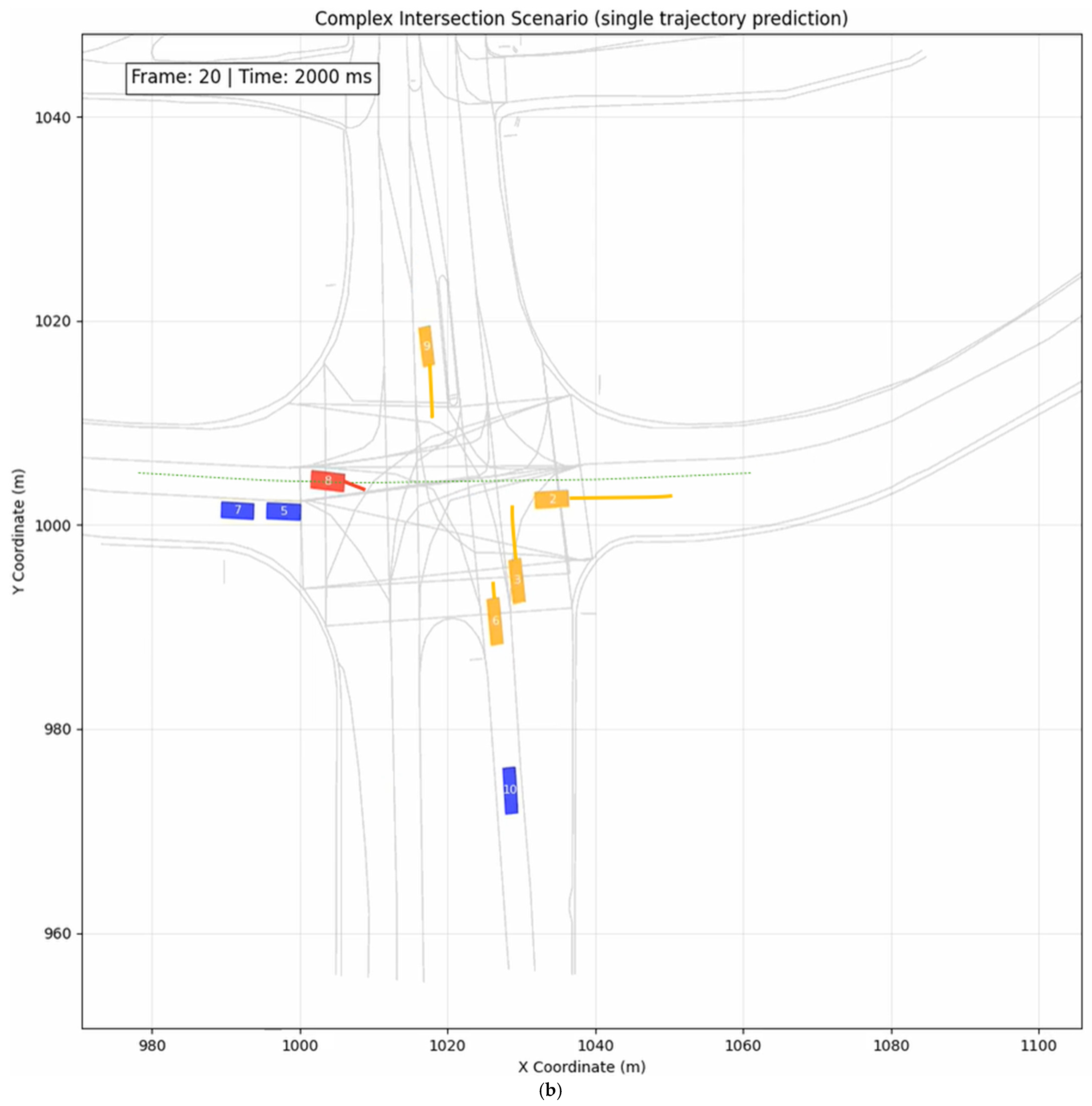
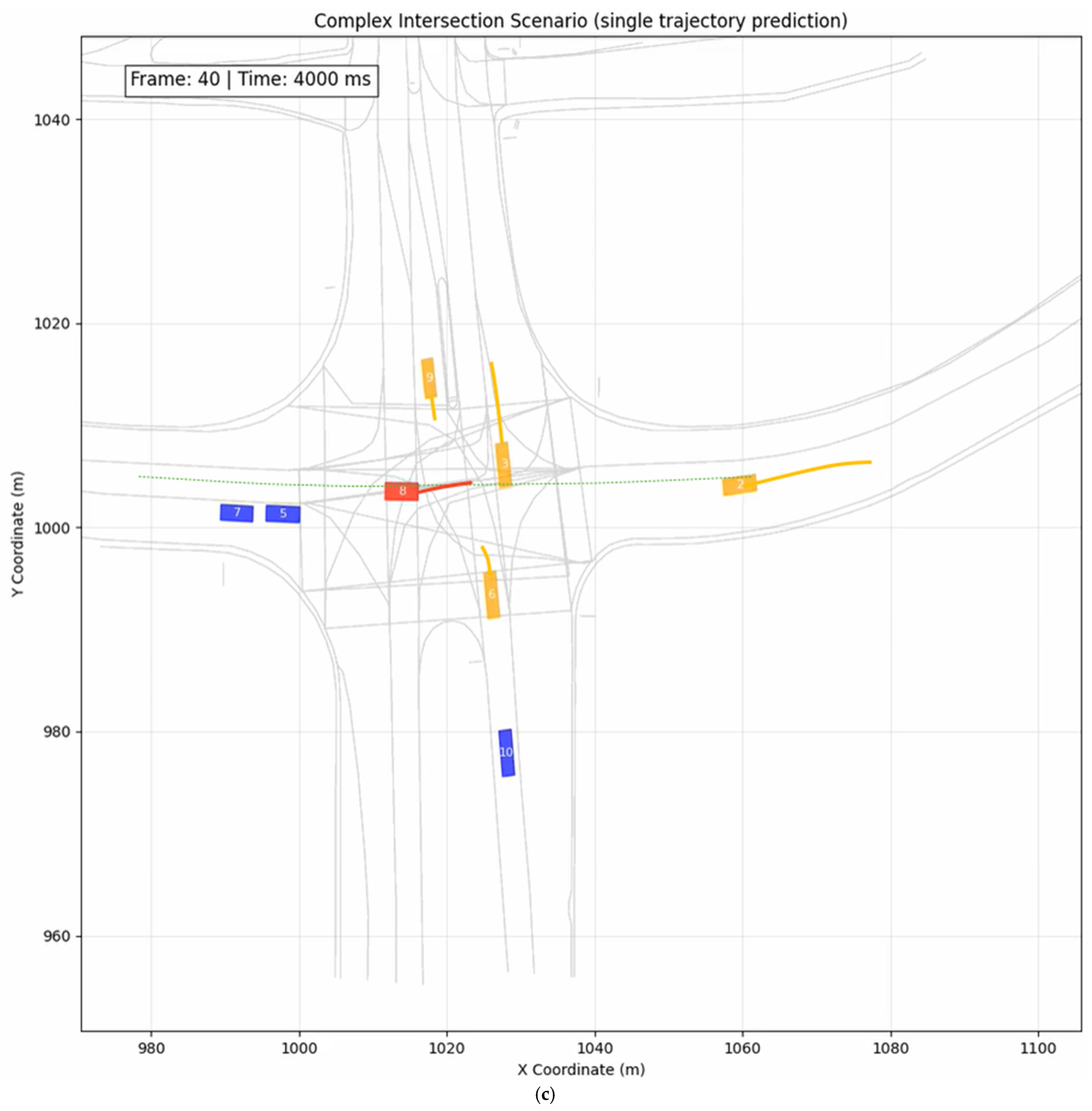
Figure 2 illustrates the evolution of vehicle positions and predictions using a single predicted trajectory per agent across three time frames (100 ms, 2000 ms, and 4000 ms) in a highly interactive intersection scenario. Initially, at the time instant of 100 ms, the prediction (shown in the green dotted line) aligns well with the immediate short-term motion of the ego vehicle, which is represented by a red block bearing the number 8. However, by 4000 ms, the prediction diverges notably from actual future positions, especially for agents undergoing complex maneuvers like turns or yielding. The single-mode assumption fails to capture potential behavioral variations, leading to inaccurate trajectory forecasts in multi-agent interactions. This demonstrates the limitations of deterministic forecasting in uncertain, dynamic environments.
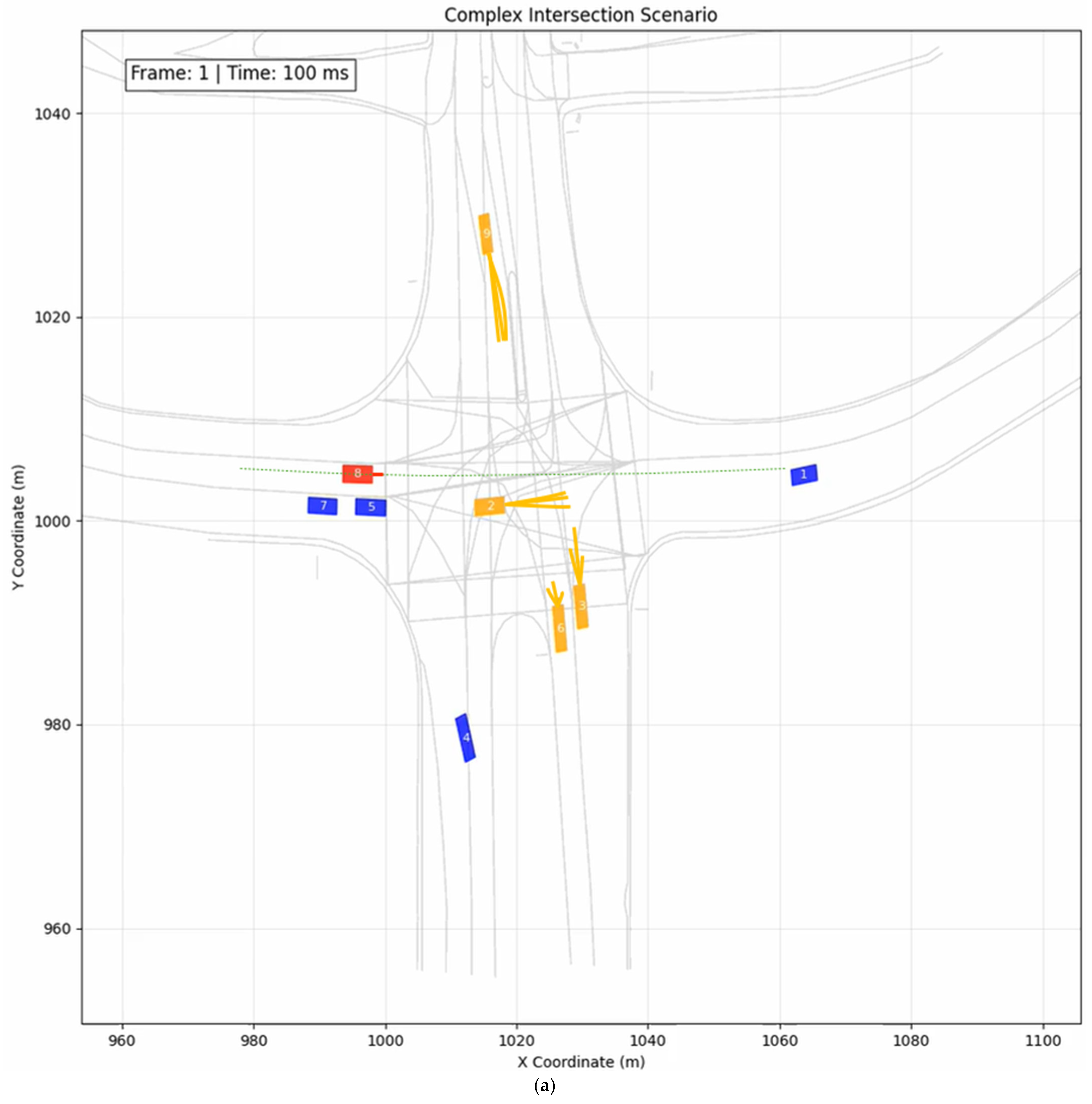
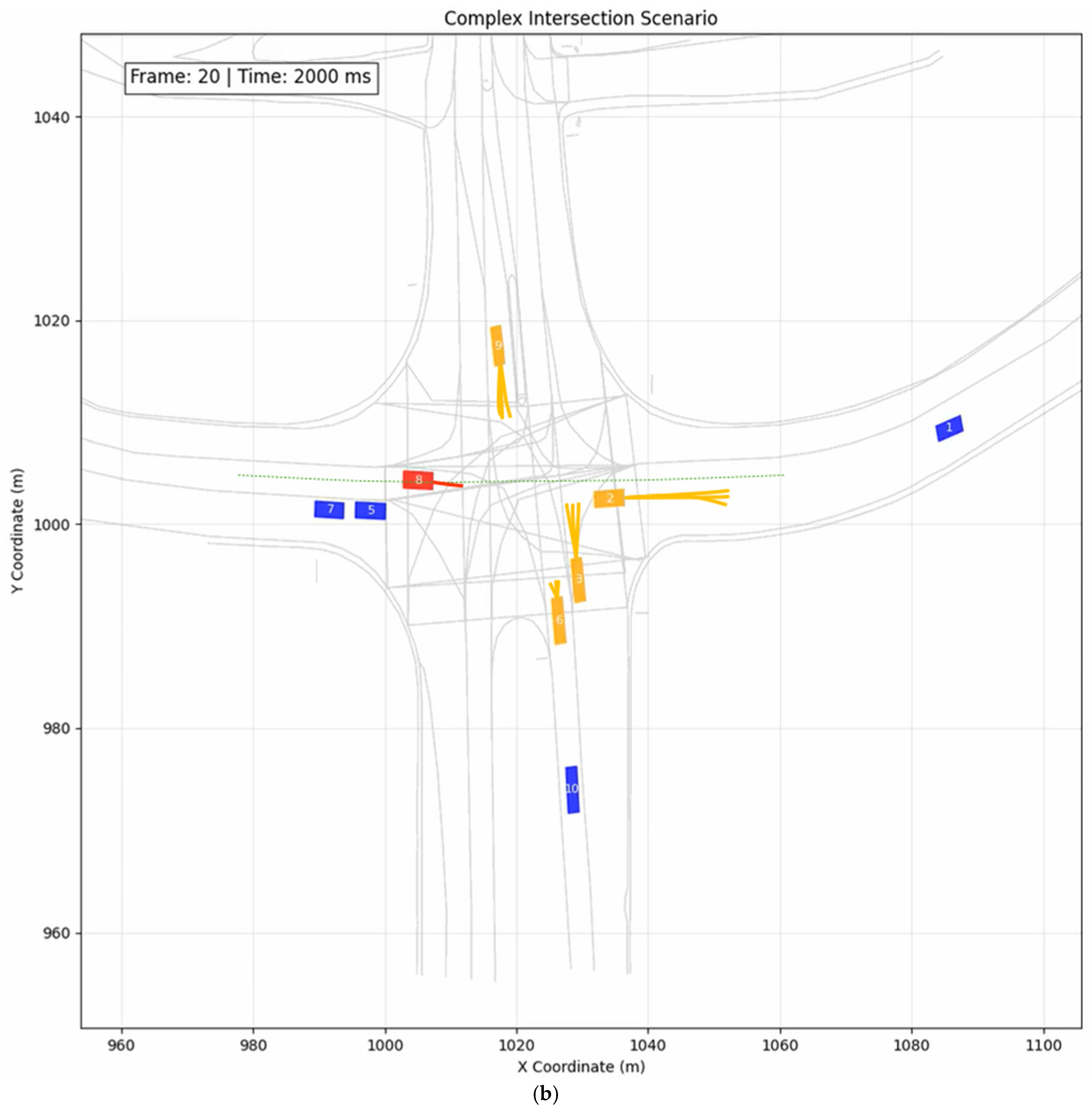
Figure 3 presents the same scenario with three predicted trajectories per agent, offering a multi-modal representation of future behavior. From the earliest time frame at 100 ms, the predictor presents diverse driving intentions, e.g., vehicles considering both left and right turns, as well as straight running. By the time of 4000 ms, the prediction branches cover a broader span of possible maneuvers, better accounting for uncertainty and interaction dynamics. The richer predictions improve coverage of likely outcomes, especially in competitive or ambiguous right-of-way situations. It enables downstream planners to make more informed, risk-aware decisions by anticipating multiple possibilities rather than a single guess.
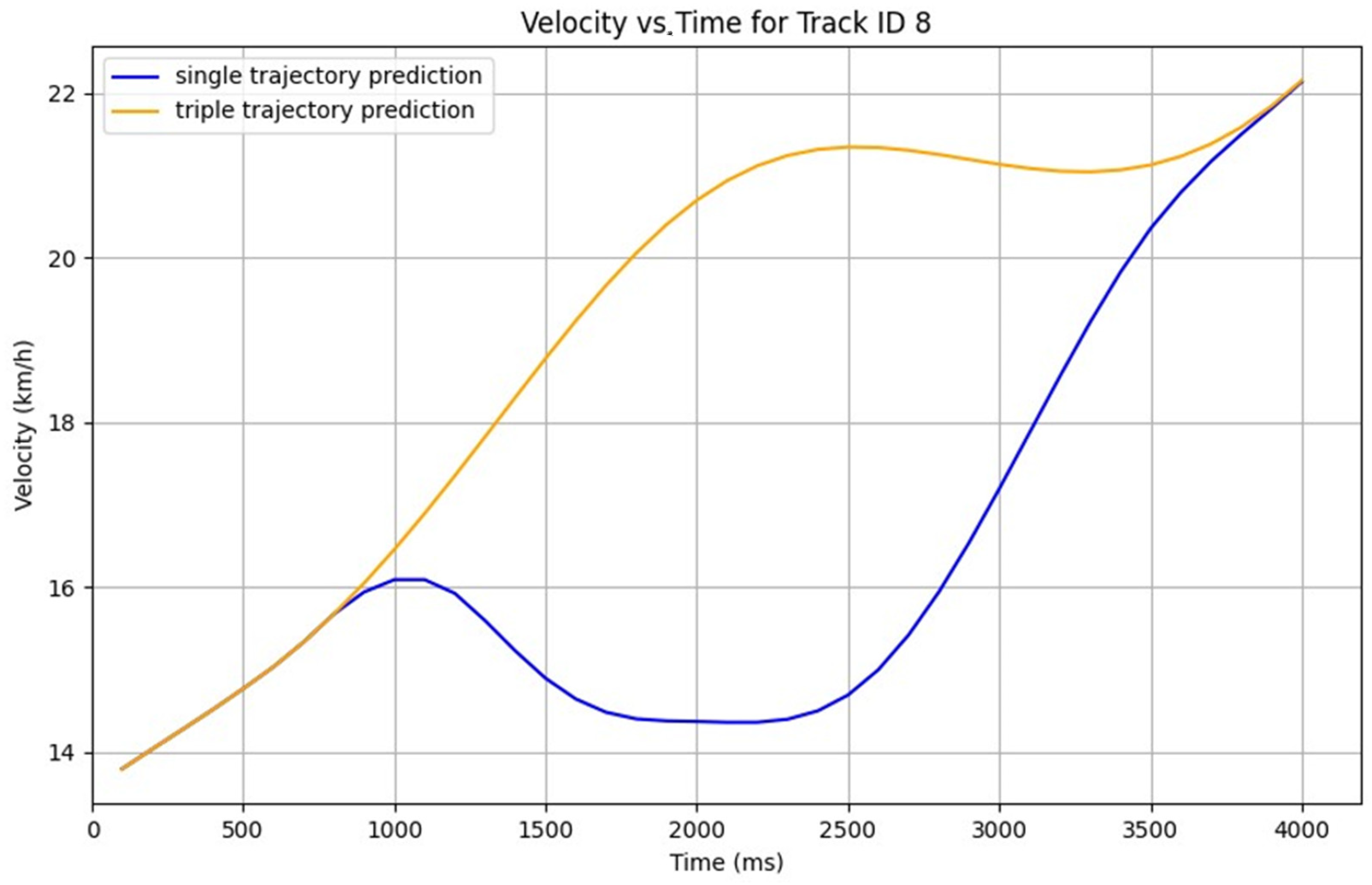
Figure 4 compares the predicted velocity profiles over the time period of 4 s for the ego vehicle under single- and triple-trajectory prediction modes. The triple-trajectory prediction (orange) exhibits a smoother and more confident velocity ramp-up, peaking earlier and maintaining higher speeds with less fluctuation. In contrast, the single-trajectory prediction (blue) shows premature acceleration, followed by an overcautious deceleration dip between 1000–3000 ms. This mismatch implies that the single trajectory prediction struggles to account for interaction uncertainty, leading to suboptimal speed planning. The triple trajectory prediction, by considering multiple plausible futures, maintains better momentum and realism in dynamic interactions; the vehicle can safely negotiate the intersection with higher average speed and smooth speed variation, thereby achieving higher transportation efficiency and better ride comfort.
Figure 5 shows the evolution of the heading angle for the same vehicle under the two prediction modes. The single-trajectory prediction (blue) produces a sharp and deep deviation in heading angle, which is over 6° from the initial heading before the variable curves back, implying a violent and possibly unrealistic steering action. In contrast, the triple-trajectory prediction (orange) permits the vehicle to remain close to the initial orientation throughout the horizon, suggesting smoother and more stable steering actions. This highlights how the multi-modal approach better captures feasible orientation evolution, avoiding violent and possibly incorrect steering operations.

5.3. Case Study 2: Unprotected Left Turn

The chosen scenario, i.e., DR_USA_Intersection_EP from the INTERACTION dataset, is a busy all-way-stop T-intersection with six branches. Vehicles approach simultaneously from multiple directions, leading to strong competition for right-of-way and frequent negotiations [21]. Drivers exhibit socially influenced behaviors like creeping forward, delayed yielding, and occasional aggressive maneuvers. The scenario reflects highly interactive and ambiguous urban dynamics, making it ideal for testing decision-making under social pressure.
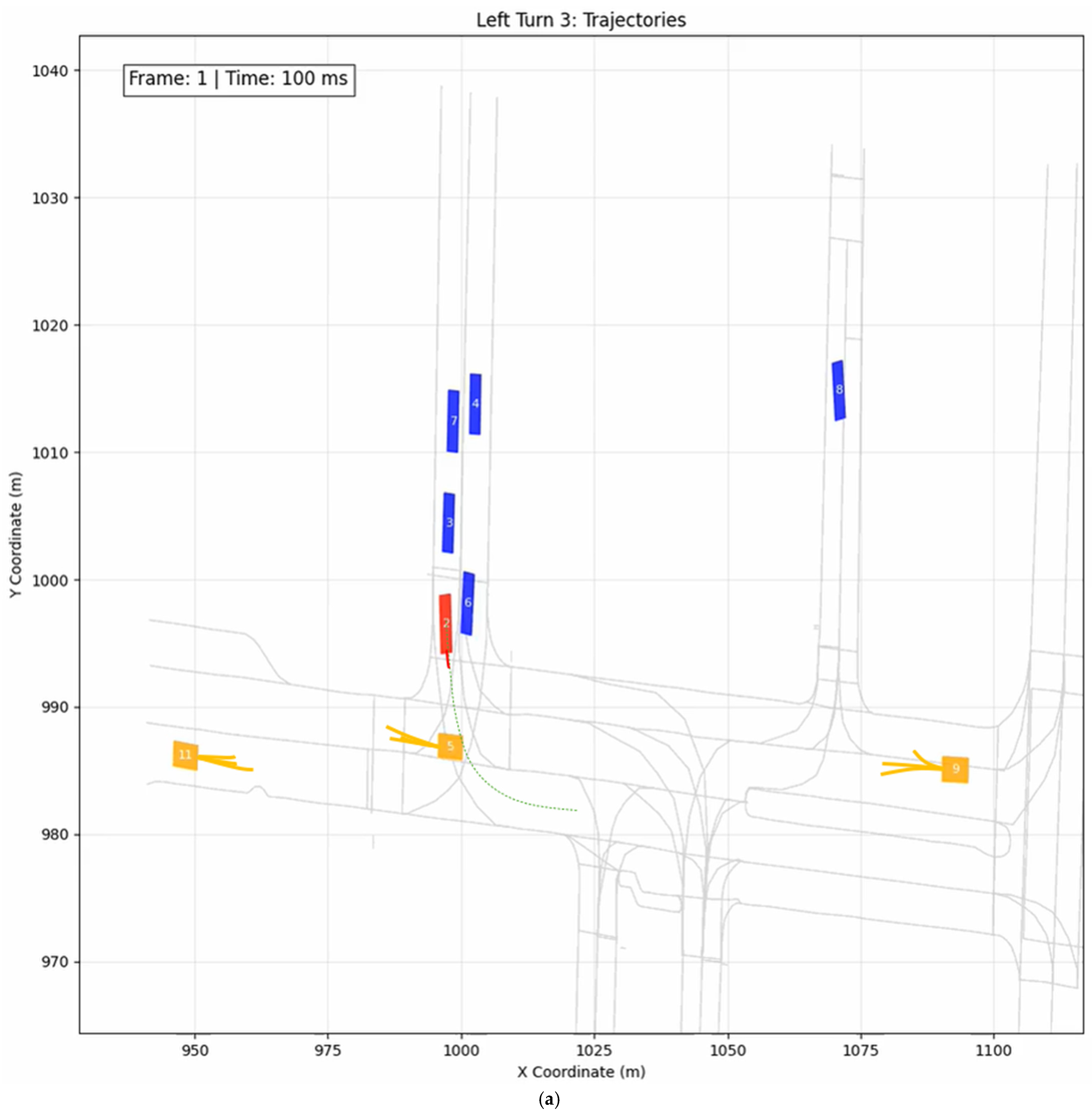
Figure 6 visualizes the predicted left-turn maneuver of the ego vehicle (represented by a red block bearing the number (2) at 100 ms, 2000 ms, and 4000 ms. The ego vehicle initiates from the lower-right lane and executes a smooth left turn across the intersection. The predicted trajectory adheres closely to the intended lane geometry while maintaining safe distances from nearby agents. Notably, surrounding vehicles exhibit cooperative behavior, adjusting their paths in response. The proposed Multi-Traj GNN-MPC planner demonstrates strong spatial foresight, generating stable, feasible trajectories without lateral deviations or abrupt shifts, highlighting the efficacy of multi-agent interaction modeling in complex urban contexts.
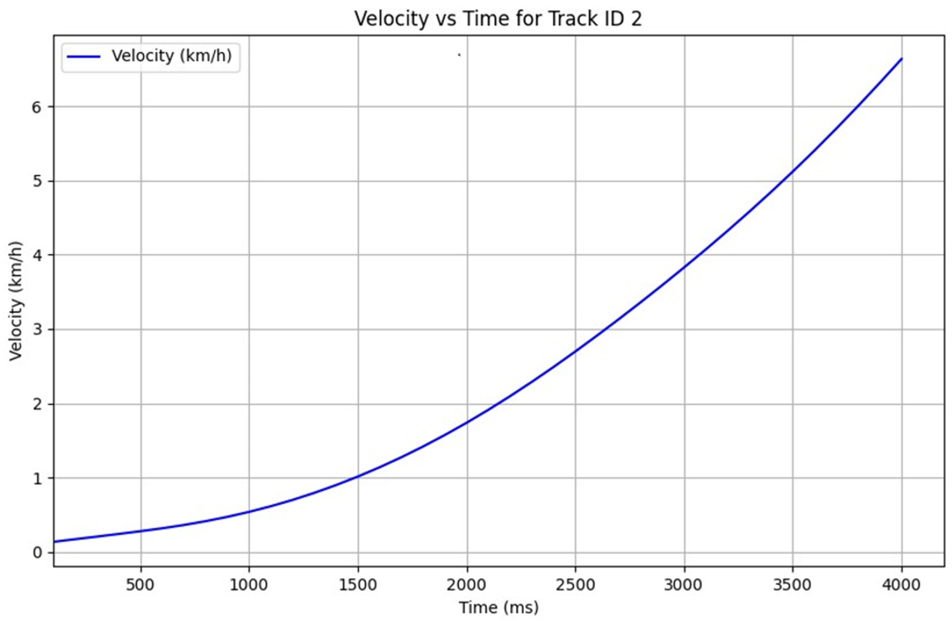
Figure 7 shows the predicted speed profile for the ego vehicle over the unprotected left turn maneuver. The time history of the vehicle’s forward speed illustrates a gradual and uninterrupted acceleration from a near standstill to approximately 6.5 km/h over a 4-s horizon. The speed profile is monotonic and free of sudden fluctuations, reflecting a confident and unimpeded maneuver. This trend is characteristic of naturalistic low-speed intersection turns and confirms that the planner outputs dynamically smooth and collision-aware control commands. The absence of speed dips or oscillations indicates that the planner successfully anticipates surrounding agents’ behaviors and does not require evasive braking.
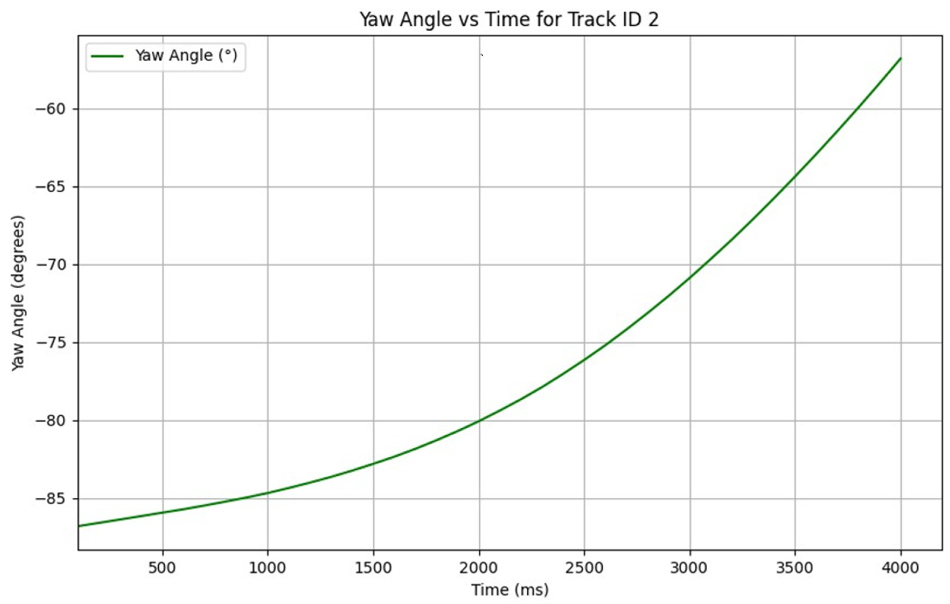
Figure 8 displays the time history of the ego vehicle’s heading angle over the unprotected left turn maneuver. The time history of the heading angle shows a consistent progression from −88° to −60°, matching the expected angular change for a left turn. The curve is smooth, continuous, and convex, with no discontinuities or overshoot. This indicates that the planner generates kinematically valid and physically realistic heading transitions. Combined with the trajectory and velocity results, the heading angle confirms that the multi-modal prediction effectively guides the planner through dynamically consistent left-turn maneuvers, even in the presence of uncertain cross-traffic behaviors.

6. Conclusions

This article presents an interaction-aware motion planning framework that integrates a GNN-based multi-modal trajectory predictor with an MPC-based motion planner. By predicting multiple plausible future trajectories for each interacting agent, the integrated motion planner enables the autonomous ego vehicle to account for different possible behaviors, e.g., yielding and aggressive driving, and to plan a motion that is safe for all those possibilities. The planner is formulated to treat the predicted primary trajectory for each of the other road users as a hard constraint, which ensures strict collision avoidance for the most likely behaviors. On the other hand, the planner treats alternate trajectories as soft constraints with heavy penalties, which allow the ego vehicle to cautiously advance when those alternate behaviors do not materialize. This formulation is shown to produce intelligent and adaptive behaviors in challenging intersection scenarios, in which the ego vehicle naturally performs common-sense driving maneuvers like creeping forward while yielding without requiring hand-coded rules.
In extensive tests on real intersection data, the multi-modal trajectory predictor consistently improves both safety and performance compared to a single-trajectory baseline predictor. The former eliminates failure cases that the latter would suffer from incorrect assumptions, and the proposed planner reduces unnecessary waiting time and abrupt motions. Quantitatively, the integrated motion planner achieves better safety distances while reducing delay by 15% and decreasing peak jerk in conflict scenarios. The planned trajectories are smoother and more in line with what a defensive yet assertive human driver would handle in the situation.
In this study, only two scenarios (i.e., (1) unsignalized intersection and (2) unprotected left turn) are considered. However, they are representative and relatively complex traffic scenarios. Most of the regular traffic scenarios are relatively simple and structured with explicit right-of-way, e.g., signalized intersections. By introducing map information with references and semantics, such as lane connections and traffic rules, we may extend the methods discussed in the article and make them generalized for other types of intersections or traffic situations.
There are several avenues to extend this study. First, the trajectory predictor could be enhanced to output probability or confidence for each mode. Second, there may be a combinatorial explosion of mode combinations. Efforts may be made to explore scenario reduction techniques, thereby focusing on a few worst-case combinations. Finally, it is expected to implement the proposed motion planner on a real vehicle or high-fidelity simulator to further validate its efficacy in live traffic, including how the ego vehicle negotiates with human drivers.

Author Contributions

Supervision, Y.H. and X.L.; conceptualization, and methodology, A.G. and Y.H.; data collection, A.G.; software, validation, investigation, and analysis, A.G.; writing original draft preparation, A.G.; writing review and editing, Y.H. and A.G. All authors have read and agreed to the published version of the manuscript.

Funding

This research was funded by a Natural Sciences and Engineering Research Council of Canada Discovery Grant (RGPIN/2019-05437-).

Data Availability Statement

The original contributions presented in this study are included in the article. Further inquiries can be directed to the corresponding author(s).

Acknowledgments

Y.H. would like to thank the team members of the Multidisciplinary Vehicle Systems Design Laboratory, University of Ontario Institute of Technology. These team members partially participated in the discussions of the results presented in the paper.

Conflicts of Interest

The authors declare no conflicts of interest.

Appendix A

The computational complexities of the proposed framework are analyzed as follows.
  • Trajectory Prediction (GNN-based Multi-Modal Prediction)
The GNN is implemented as an edge-conditioned message-passing neural network with L layers. For a scene graph with N agents and E directed edges, and latent feature dimension d, the per-layer complexity is
O (E  d2)
Therefore, for L layers, the GNN encoder’s total complexity is
O (L  E  d2)
Since we predict M trajectory modes per agent using M parallel MLP decoders, each of complexity O (H d2) for prediction horizon H, the total decoder complexity is
O (M N  H  d2)
Thus, the total complexity of the predictor is
O (L E  d2+ M N H d2)
In our evaluation, L = 3, M = 3, H = 15, and d = 64, with up to N = 10, so inference remains within 25 ms on a GPU.
2.
Motion Planning (NMPC with IPOPT)
The planner solves an NMPC problem over horizon H with four states and two control variables. For each planning cycle, the complexity of interior-point optimization via IPOPT scales with the number of variables and constraints. Let nx = 4 (number of state variables), nu = 2 (number of control variables), H = 15 (planning horizon), and K = 8 (number of nonlinear constraints). The number of decision variables is (nx + nu) H, so the worst-case complexity is
O (((nx + nu) H)3+ K)
However, in practice, IPOPT exploits sparsity and warm starts, reducing the effective runtime. Empirically, the solver completes in 25–40 ms on a desktop CPU for our setup.
3.
End-to-End Framework Complexity
Combining both modules, the overall computational complexity per cycle is
O (L E  d2  +M  N  H  d2+ ((nx+nu) H)3+ K)
Given that all constants are fixed and small in our use case (e.g., N < 10, H = 15), the framework is real-time capable at 5 Hz, as demonstrated on our hardware. This explicit complexity now precisely characterizes the scalability and runtime profile of our integrated prediction and planning method.

References

  1. Yang, K.; Tang, X.; Li, J.; Wang, H.; Zhong, G.; Chen, J. Uncertainties in Onboard Algorithms for Autonomous Vehicles: Challenges, Mitigation, and Perspectives. IEEE Trans. Intell. Transp. Syst. 2023, 24, 8963–8987. [Google Scholar] [CrossRef]
  2. Sánchez, M.M.; Silvas, E.; Elfring, J.; van de Molengraft, R. Robustness Benchmark of Road User Trajectory Prediction Models for Automated Driving. IFAC-PapersOnLine 2023, 56, 4865–4870. [Google Scholar] [CrossRef]
  3. Zhang, X.; Zeinali, S.; Schildbach, G. Interaction-aware Traffic Prediction and Scenario-based Model Predictive Control for Autonomous Vehicle on Highways. In Proceedings of the 2024 European Control Conference (ECC), Stockholm, Sweden, 25–28 June 2024; pp. 3344–3350. [Google Scholar]
  4. Aradi, S. Survey of Deep Reinforcement Learning for Motion Planning of Autonomous Vehicles. IEEE Trans. Intell. Transp. Syst. 2022, 23, 740–759. [Google Scholar] [CrossRef]
  5. Paden, B.; Čáp, M.; Yong, S.Z.; Yershov, D.; Frazzoli, E. A Survey of Motion Planning and Control Techniques for Self-driving Urban Vehicles. IEEE Trans. Intell. Veh. 2016, 1, 33–55. [Google Scholar] [CrossRef]
  6. Schwarting, W.; Alonso-Mora, J.; Rus, D. Planning and Decision-making for Autonomous Vehicles. Annu. Rev. Control Robot. Auton. Syst. 2018, 1, 187–210. [Google Scholar] [CrossRef]
  7. Xin, L.; Wang, P.; Chan, C.Y.; Chen, J.; Li, S.E.; Cheng, B. Intention-aware Long Horizon Trajectory Prediction of Surrounding Vehicles Using Dual LSTM Networks. In Proceedings of the 2018 21st International Conference on Intelligent Transportation Systems (ITSC), Maui, HI, USA, 4–7 November 2018; pp. 1441–1446. [Google Scholar]
  8. Deo, N.; Trivedi, M.M. Convolutional Social Pooling for Vehicle Trajectory Prediction. In Proceedings of the IEEE Conference on Computer Vision and Pattern Recognition (CVPR) Workshops, Salt Lake City, UT, USA, 18–22 June 2018; pp. 1468–1476. [Google Scholar]
  9. Diehl, F.; Brunner, T.; Le, M.T.; Knoll, A. Graph Neural Networks for Modelling Traffic Participant Interaction. In Proceedings of the 2019 IEEE Intelligent Vehicles Symposium (IV), Paris, France, 9–12 June 2019; pp. 695–701. [Google Scholar]
  10. Mo, X.; Huang, Z.; Xing, Y.; Lv, C. Multi-agent Trajectory Prediction with Heterogeneous Edge-enhanced Graph Attention Network. IEEE Trans. Intell. Transp. Syst. 2022, 23, 9554–9567. [Google Scholar] [CrossRef]
  11. Sun, Q.; Huang, X.; Gu, J.; Williams, B.C.; Zhao, H. M2I: From Factored Marginal Trajectory Prediction to Interactive Prediction. In Proceedings of the IEEE/CVF Conference on Computer Vision and Pattern Recognition (CVPR), New Orleans, LA, USA, 18–24 June 2022; pp. 6533–6542. [Google Scholar]
  12. Gautam, A.; He, Y.; Lin, X. An Overview of Motion-planning Algorithms for Autonomous Ground Vehicles with Various Applications. SAE Int. J. Veh. Dyn. Stab. NVH 2024, 8, 179–213. [Google Scholar] [CrossRef]
  13. Qian, X.; Navarro, I.; de La Fortelle, A.; Moutarde, F. Motion Planning for Urban Autonomous Driving Using Bezier Curves and MPC. In Proceedings of the 2016 IEEE 19th International Conference on Intelligent Transportation Systems (ITSC), Rio de Janeiro, Brazil, 1–4 November 2016; IEEE: Piscataway, NJ, USA, 2016; pp. 826–833. [Google Scholar]
  14. Sharma, T.; He, Y. Design of a Tracking Controller for Autonomous Articulated Heavy Vehicles Using a Nonlinear Model Predictive Control Technique. Proc. Inst. Mech. Eng. Part. K J. Multibody Dyn. 2024, 238, 334–362. [Google Scholar] [CrossRef]
  15. Rasekhipour, Y.; Khajepour, A.; Chen, S.K.; Litkouhi, B. A Potential Field-based Model Predictive Path-planning Controller for Autonomous Road Vehicles. IEEE Trans. Intell. Transp. Syst. 2016, 18, 1255–1267. [Google Scholar] [CrossRef]
  16. Testouri, M.; Elghazaly, G.; Frank, R. Towards a Safe Real-Time Motion Planning Framework for Autonomous Driving Systems: A Model Predictive Path Integral Approach. In Proceedings of the 2023 3rd International Conference on Robotics, Automation and Artificial Intelligence (RAAI), Singapore, 14–16 December 2023; pp. 231–238. [Google Scholar]
  17. Bae, S.; Isele, D.; Nakhaei, A.; Xu, P.; Añon, A.M.; Choi, C. Lane-change in Dense Traffic with Model Predictive Control and Neural Networks. IEEE Trans. Control. Syst. Technol. 2023, 31, 646–659. [Google Scholar] [CrossRef]
  18. Sheng, Z.; Liu, L.; Xue, S.; Zhao, D.; Jiang, M.; Li, D. A Cooperation-aware Lane Change Method for Automated Vehicles. IEEE Trans. Intell. Transp. Syst. 2023, 24, 3236–3251. [Google Scholar] [CrossRef]
  19. Gupta, P.; Isele, D.; Lee, D.; Bae, S. Interaction-aware Trajectory Planning for Autonomous Vehicles with Analytic Integration of Neural Networks into Model Predictive Control. In Proceedings of the 2023 IEEE International Conference on Robotics and Automation (ICRA), London, UK, 29 May–2 June 2023; pp. 7794–7800. [Google Scholar]
  20. INTERACTION Dataset. 2025. Available online: https://interaction-dataset.com/ (accessed on 19 July 2025).
  21. Zhan, W.; Sun, L.; Wang, D.; Shi, H.; Clausse, A.; Naumann, M.; Kummerle, J.; Konigshof, H.; Stiller, C.; de La Fortelle, A.; et al. INTERACTION Dataset: An International, Adversarial and Cooperative Motion Dataset in Interactive Driving Scenarios with Semantic Maps. arXiv 2019, arXiv:1910.03088. [Google Scholar] [CrossRef]
  22. The Autoware Foundation. Available online: https://autoware.org/ (accessed on 20 July 2025).
  23. Pivtoraiko, M.; Kelly, A. Generating Near Minimal Spanning Control Sets for Constrained Motion Planning in Discrete State Spaces. In Proceedings of the 2005 IEEE/RSJ International Conference on Intelligent Robots and Systems, Edmonton, AB, Canada, 2–6 August 2005; IEEE: Piscataway, NJ, USA, 2005; pp. 3231–3237. [Google Scholar]
  24. Andersson, J.; Gillis, J. CasADi Documentation (PDF version). Release 3.7.1. 23 July 2025. Available online: https://web.casadi.org/docs/ (accessed on 26 July 2024).
  25. IPOPT Documentation. Available online: https://coin-or.github.io/Ipopt/index.html (accessed on 25 June 2024).
  26. Bi-Directional Gated Recurrent Unit. Available online: https://www.sciencedirect.com/topics/computer-science/bi-directional-gated-recurrent-unit (accessed on 26 June 2024).
  27. Gao, J.; Sun, C.; Zhao, H.; Shen, Y.; Anguelov, D.; Li, C.; Schmid, C. VectorNet: Encoding HD Maps and Agent Dynamics from Vectorized Representation. In Proceedings of the IEEE/CVF Conference on Computer Vision and Pattern Recognition (CVPR), Seattle, WA, USA, 13–19 June 2020; pp. 11525–11533. [Google Scholar]
  28. Mao, C.; He, Y.; Agelin-Chaab, M. A Design Method for Road Vehicles with Autonomous Driving Control. Actuators 2024, 13, 427. [Google Scholar] [CrossRef]
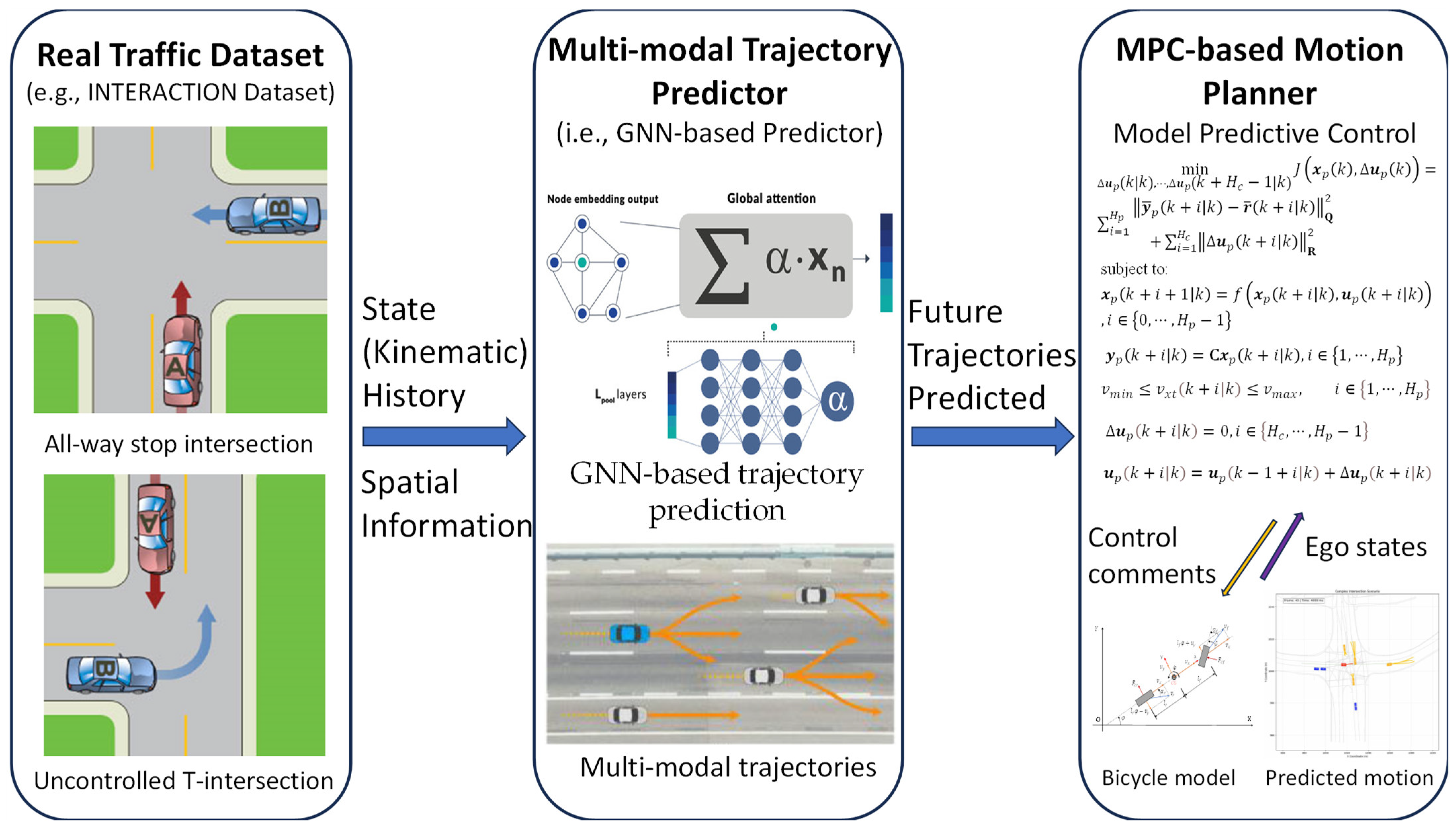
Figure 1. Architecture of the integrated motion planning algorithm.
Machines 13 00760 g001
Figure 2. Single trajectory prediction at an unsignalized all-way stop intersection at different time instants: (a) 100 ms; (b) 2000 ms; (c) 4000 ms. Note that the red block represents the ego vehicle, the yellow blocks denote the obstacle vehicles that closely interact with the ego vehicle, and the blue blocks indicate the obstacle vehicles that loosely interact with the ego vehicle.
Machines 13 00760 g002aMachines 13 00760 g002bMachines 13 00760 g002c
Figure 3. Triple trajectory prediction at an unsignalized all-way stop intersection at different time instants: (a) 100 ms; (b) 2000 ms; (c) 4000 ms. Note that the red block represents the ego vehicle, the yellow blocks denote the obstacle vehicles that closely interact with the ego vehicle, and the blue blocks indicate the obstacle vehicles that loosely interact with the ego vehicle.
Machines 13 00760 g003aMachines 13 00760 g003bMachines 13 00760 g003c
Figure 4. Time histories of the ego vehicle’s forward speed derived from the Multi-Traj GNN-MPC planner and Single-Traj MPC baseline planner.
Machines 13 00760 g004
Figure 5. Time histories of the ego vehicle’s heading angle derived from the Multi-Traj GNN-MPC planner and Single-Traj MPC baseline planner.
Machines 13 00760 g005
Figure 6. Vehicles’ states at the unprotected left turn at different time instants: (a) 100 ms; (b) 2000 ms; (c) 4000 ms. Note that the red block represents the ego vehicle, the yellow blocks denote the obstacle vehicles that closely interact with the ego vehicle, and the blue blocks indicate the obstacle vehicles that loosely interact with the ego vehicle.
Machines 13 00760 g006aMachines 13 00760 g006bMachines 13 00760 g006c
Figure 7. Time history of the forward speed of the ego vehicle.
Machines 13 00760 g007
Figure 8. Time history of heading angle of the ego vehicle.
Machines 13 00760 g008
Table 1. Parameters for the vehicle model and the MPC-based motion planner.
ParameterValueParameterValue
Distance between vehicle CG and its front axle l f 1.33 mDistance between vehicle CG and its front axle l f 1.81 m
Radius of circle representing ego vehicle R e g o 1.5 mRadius of circle representing vehicle A i R i 1.5 m
Total number of sampling time step T f 15Duration of one-time step t 0.2 s
Maximum acceleration a m a x 2.5   m / s 2 Maximum deceleration a m i n 6.0   m / s 2
Maximum front-wheel steering angle δ m a x 39.6 o Maximum vehicle forward-speed v m a x 15   m / s
Maximum permitted lateral deviation y d e v 0.5   m Required ego vehicle speed at stop v 0.0 m/s
Reference ego vehicle speed for different cases * v r e f 8 ,   0 ,   5   m / s Prediction horizon H p 15
Control horizon H c 15Weighting factor for position deviation q p o s 130
Weighting factor for heading angle deviation q ϕ 130Weighting factor for speed deviation q v e l 4
Weighting factor for acceleration q a 6Weighting factor for steering angle q δ 100
Weighting factor for acceleration variation q Δ a 50Weighting factor for steering angle variation q Δ δ 10
Weighting factor for slack term q 10 6
* Reference ego vehicle speed v r e f while approaching an interaction, at the stop line, and in a left turn are 8, 0, and 5 m/s, respectively.
Disclaimer/Publisher’s Note: The statements, opinions and data contained in all publications are solely those of the individual author(s) and contributor(s) and not of MDPI and/or the editor(s). MDPI and/or the editor(s) disclaim responsibility for any injury to people or property resulting from any ideas, methods, instructions or products referred to in the content.