Article

Optimizing Random Forest with Hybrid Swarm Intelligence Algorithms for Predicting Shear Bond Strength of Cable Bolts

1
School of Resources and Safety Engineering, Central South University, Changsha 410083, China
2
Institute of Innovation, Science and Sustainability, Federation University Australia, Ballarat, VIC 3350, Australia
3
Laboratory of Sustainable Development in Natural Resources and Environment, Institute for Advanced Study in Technology, Ton Duc Thang University, Ho Chi Minh City 700000, Vietnam
4
Faculty of Environment and Labour Safety, Ton Duc Thang University, Ho Chi Minh City 700000, Vietnam
5
Department of Mining Engineering, Isfahan University of Technology, Isfahan 8415683111, Iran
*
Authors to whom correspondence should be addressed.
Machines 2025, 13(9), 758; https://doi.org/10.3390/machines13090758
Submission received: 13 July 2025 / Revised: 13 August 2025 / Accepted: 19 August 2025 / Published: 24 August 2025
(This article belongs to the Special Issue Key Technologies in Intelligent Mining Equipment)

Abstract

This study combines three optimization algorithms, Tunicate Swarm Algorithm (TSA), Whale Optimization Algorithm (WOA), and Jellyfish Search Optimizer (JSO), with random forest (RF) to predict the shear bond strength of cable bolts under different types and grouting conditions. Based on the original dataset, a database of 860 samples was generated by introducing random noise around each data point. After establishing three hybrid models (RF-WOA, RF-JSO, RF-TSA) and training them, the obtained models were evaluated using six metrics: coefficient of determination (R2), root mean squared error (RMSE), mean absolute error (MAE), mean absolute percentage error (MAPE), variance account for (VAF), and A-20 index. The results indicate that the RF-JSO model exhibits superior performance compared to the other models. The RF-JSO model achieved an excellent performance on the testing set (R2 = 0.981, RMSE = 11.063, MAE = 6.457, MAPE = 9, VAF = 98.168, A-20 = 0.891). In addition, Shapley Additive exPlanations (SHAP), Partial Dependence Plot (PDP), and Local Interpretable Model-agnostic Explanations (LIME) were used to analyze the interpretability of the model, and it was found that confining pressure (Stress), elastic modulus (E), and a standard cable type (cable type_standard) contributed the most to the prediction of shear bond strength. In summary, the hybrid model proposed in this study can effectively predict the shear bond strength of cable bolts.

1. Introduction

The cable bolts are widely used to reinforce and stabilize rocks [1]. They are made by binding multiple steel wires together, creating strands that provide flexibility [2]. Due to their easy installation, affordability, minimal space requirements during excavation, adaptability, and high bearing capacity, they are extensively used in mining engineering. Extensive pull-out tests have consistently substantiated that the slip occurring along the bolt–grout interface constitutes the primary mode of damage for the cable bolts [3]. Consequently, the shear bond stiffness between the bolts and the grout is essential for assessing the extent of bolt damage.
Historically, investigations into the deformation and failure processes, along with the load transfer mechanisms of anchor cables subjected to tensile loading, have been conducted through experimental studies, numerical simulations, and analytical modeling approaches.
Extensive laboratory and in situ pull-out tests have provided invaluable empirical data, revealing the critical influence of factors such as confining pressure and embedment length. Salcher et al. [4] conducted extensive pull-out tests on Sydney sandstones and shales and concluded that consistent stiffness was observed in cement-grouted bolts within sandstone, and the stiffness increase was correlated with the aperture. Thenevin et al. [5] introduced an extensive laboratory pull-out test results database, confirming how confining pressure and embedment length influence the pull-out response behaviors. However, these experimental approaches are often time-consuming, costly, and their findings are constrained to the specific geological and material conditions tested, limiting their generalizability.
To overcome these limitations, researchers have developed various analytical and numerical models. Fu et al. [6] established a relationship model for the anchoring force of hard surrounding rock based on the main slip interface. Chen et al. [7] propose a numerical method for estimating the largest confinement cable bolts pull-out tests, simulating the pull-out performance of common and modified cable bolts. Jahangir et al. [1] defined a general method for developing a rheological interface model. The proposed method introduced a bolt–grout interface constitutive model featuring yield criteria and unrelated plastic potential, which satisfies thermodynamic conditions. Xu et al. [3] integrated the tri-linear tensile model of cable bolts and the tri-linear shear model of bolt–grout interface, defined the maximum value of the failure approach index (FAI) for bolt tensile failure and the maximum value of FAI for B-G interface shear failure, and effectively quantified the safety of cable bolts. Chen et al. [8] developed an analytical model to predict the load transfer behavior of fully grouted cable bolts under axial loads. The model is based on a trilinear model describing the shear characteristics of the anchor slurry interface. Nourizadeh et al. [9] performed push tests on cubic specimens under triaxial conditions by applying non-uniform confining stress. The tests revealed the impact of confinement conditions on the system and the failure mechanism of specimens under varying conditions. While these models offer significant insights into the mechanics of bolt–grout interaction, they frequently rely on idealized assumptions. As a result, their predictive accuracy can be compromised when dealing with the high-dimensional, nonlinear, and complex relationships inherent in real-world rock engineering applications.
With the development of artificial intelligence and machine learning, many researchers have begun to use machine learning methods to study problems in geotechnical engineering [10,11,12,13]. Machine learning models can handle high-dimensional, nonlinear, and complex relationships. This capability allows for the more comprehensive utilization of vast amounts of experimental and scenario data, leading to a more accurate and holistic model. Ali et al. [14] established an artificial neural network for modeling the load-displacement curve of fully grouted cable bolts. The network accurately captures the bolt/grout mass interactions, and the proposed model’s effectiveness is validated through pull-out test results. Shokri et al. [15] proposed the use of the XGBoost model to predict the axial load-bearing capacity of fully grouted rock bolting systems, achieving satisfactory results. Soufi et al. [16] proposed a novel artificial neural network (ANN) model that utilizes data from in situ pull-out tests to optimize cable bolt design. The proposed model demonstrated excellent predictive accuracy. Although the feasibility of machine learning has been established, many studies either employ standard algorithms with default settings or use optimization techniques that may not fully exploit the model’s predictive potential, and they often lack a corresponding interpretability analysis.
Therefore, this study introduces a method based on a random forest model optimized by the Tunicate Swarm Algorithm (TSA), Jellyfish Search Optimizer (JSO), and Whale Optimization Algorithm (WOA), and the models are trained by using Bouteldja et al. [17]’s pull-out experiment database for predicting the shear bond strength of cable bolts under different types and grouting conditions. The obtained model predicts accurately, and the results are satisfactory. The primary contributions of this work are as follows: (1) This study evaluates the application of three distinct hybrid swarm intelligence algorithms, TSA, WOA, and JSO, for optimizing the hyperparameters of a random forest model to predict the shear bond strength of cable bolts; (2) This study provides a systematic comparison of the resulting hybrid models to identify a robust predictive approach and quantify its performance relative to a conventional random forest; and (3) This study employs explainable AI (XAI) methods, specifically SHAP and LIME, to interpret the predictions of the developed model, thereby providing insights into the relative importance of key influencing factors.

2. Methods

This study employs random forest for regression prediction and utilizes the following three metaheuristic algorithms to optimize its hyperparameters.

2.1. Random Forest (RF)

Breiman [18] proposed the random forest (RF) algorithm in 2001, which combines numerous decision trees to surpass the performance of a single decision tree. RF exhibits a straightforward structure, is easy to implement, and performs well in regression and classification problems, contributing to its widespread popularity. As shown in Figure 1, a single decision tree will serve as the basic unit in the RF structure. During the operation of RF, a certain number of decision trees will be generated, and each decision tree will obtain feature information from the provided data. Then, it will split based on the predefined minimum leaf node error (such as mean square error, MSE). This process continues until no more features are available to extend the branches and leaves of the decision tree. The final result of the RF is obtained by averaging the outcomes of all decision trees. This process is described by the following equation:
f K = 1 K K = 1 K t i ( x )
where f k   stands for RF model, t i ( x )   is a single decision tree, and K represents the total number of decision trees.
This study utilized five hyperparameters for the RF. They include n_estimators, representing the number of decision trees; max_depth, indicating the maximum depth of each tree; min_samples_split, specifying the minimum number of samples contained in each internal node (non-leaf node); min_samples_leaf, indicating the minimum number of samples for leaf nodes; and max_features, representing the number of features to consider when limiting branching. Among these parameters, n_estimators plays a crucial role in performance. The number of trees must be appropriate; too few trees may result in poor predictive performance, while too many trees not only fail to significantly enhance performance but also extend the training time due to increased computational complexity [19]. The remaining four parameters are all used to prevent overfitting of the model by restricting the growth of decision tree branches and leaves [20].

2.2. Tunicate Swarm Algorithm (TSA)

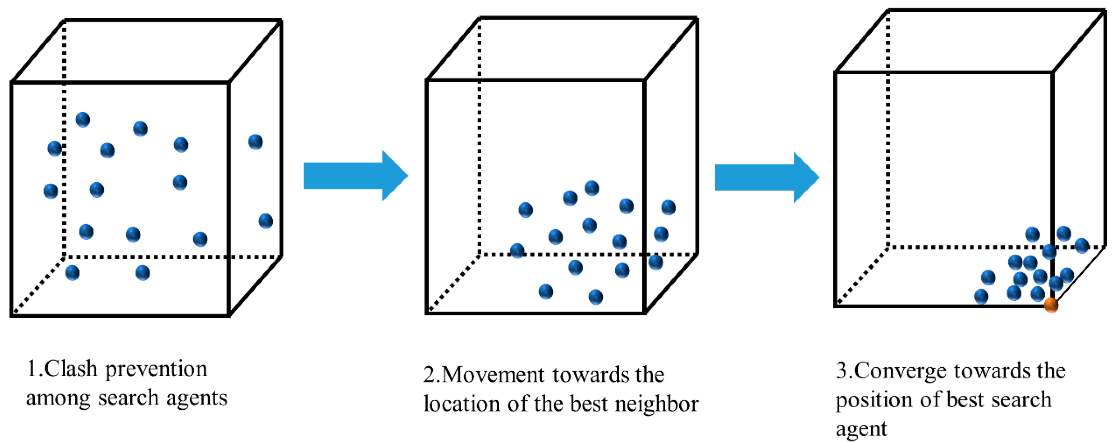
Tunicate Swarm Algorithm(TSA) was proposed by Kaur et al. [21]. Its operation process simulates the movement of deep-sea tunicate creatures by jetting seawater and the swarm intelligence they exhibit. The process of jetting seawater for movement is divided into three parts: preventing clashes among search agents, moving towards the location of the best one, and maintaining proximity to it [19]. The search process of TSA is shown in Figure 2.
(1) Prevent clashes among search agents
To prevent clashes among search agents, Vector A is used to calculate new search agent positions.
A = G M
G = c 2 + c 3 2 c 1
M = P min + c 1 P max P min
Here, G represents gravity, and M is the interaction social force between individuals in the population; c1, c2, and c3 are random numbers with values that lie in the interval [0, 1]. P min and P max are both constants [21].
(2) Move towards the location of the best neighbor
After avoiding clashes among individuals in the population, the next step is guiding individuals toward the best neighbor.
P D = F S r a n d P p ( t )
where PD represents the distance between the individual and the target, FS denotes the target, P ( t )   signifies the position of the tunicate in the current iteration, t represents the position of the individual, and rand is a random number within the range [0, 1].
(3) Converge towards the position of the best search agent
The process of search agents gradually approaching the best agent is represented by the following equation:
P p ( t ) = F S + A · P D , i f   r a n d 0.5 F S A · P D , i f   r a n d < 0.5
(4) Swarm behavior
Utilize the best positions of the first two individuals in the population as a reference, then adjust the positions of the remaining individuals accordingly. This process is represented by the following equation:
P P ( t + 1 ) = P p ( t ) + P p ( t + 1 ) 2 + c 1

2.3. Whale Optimization Algorithm (WOA)

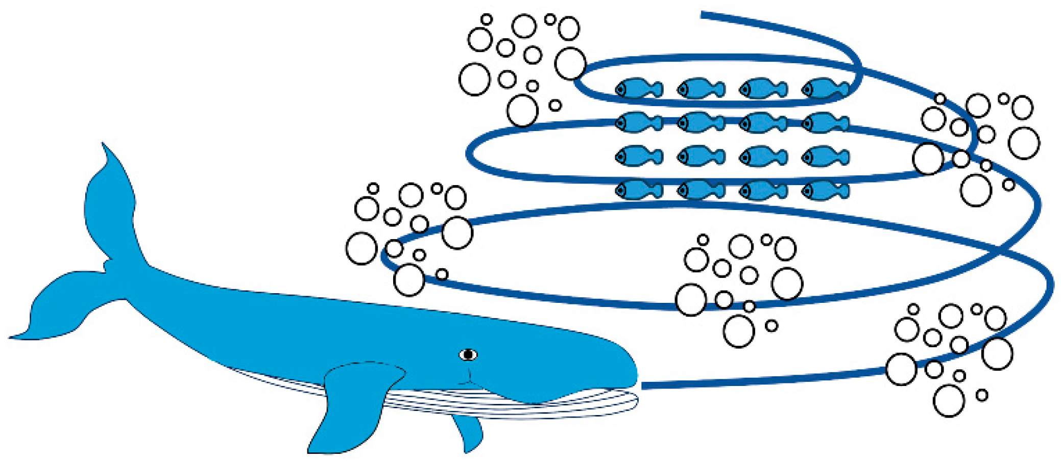
Mirjalili et al. [22] proposed the Whale Optimization Algorithm(WOA), a novel metaheuristic optimization algorithm, in 2016. This algorithm optimizes by simulating the hunting process of humpback whales. The specific implementation method mimics the bubble-net feeding method of humpback whales through a spiral [23]. The bubble-net feeding method consists of three steps: surround the prey, create a spiral bubble-net to attack the prey, and search for the next prey [19]. This process is shown in Figure 3.
(1) Surround the prey
The optimization process begins by randomly distributing individuals in the solution space. Afterwards, it is assumed that the current best solution is located near the target prey. After determining the position of the optimal candidate solution in the ongoing iteration, other search agents will adapt their positions to move closer to the optimal search agent. This sequence is shown by the following equations:
X ( t + 1 ) = X g b e s t ( t ) A · C · X g b e s t ( t ) X ( t )
A = 2 a · r a
C = 2 · r
X     signifies the position vector of the search agent, X gbest   signifies the position vector of the optimal solution in the ongoing iteration, t represents the ongoing iteration, and A   and C   are vectors of coefficients. The vector a     linearly diminishes from 2 to 0 throughout the iteration process, and r     is a random vector within the range [0, 1].
(2) Bubble-net attacking method
The bubble-net attack executed by a humpback whale can be described through a contracting surrounding mechanism and a spiral position update. Reducing the value of a     in Equation (9), the contracting surrounding mechanism can be attained. In Equation (9), it is evident that A   decreases as a     decreases. As a     diminishes from 2 to 0, the value range of A     falls within the range of [− a   , a   ]. Additionally, assigning a random value for A   within the interval [−1, 1] allows the definition of the new position X ( t + 1 )   anywhere between the current position X ( t ) and   X gbest ( t ) [22].
The spiral update of the search agent location is achieved by imitating the spiral movement of humpback whales approaching prey during hunting, which can be described by the following equation:
X ( t + 1 ) = X g b e s t ( t ) + X g b e s t ( t ) X ( t ) · e b t · cos 2 π l
where b is the constant that manages the form of the logarithmic spiral, and l is a random value within the range of [−1, 1]. To imitate the conduct of a humpback whale circling its prey within a contracted circle and along a spiral trajectory, this study hypothesizes a 50% chance of selecting either a contracting surround mechanism or a spiral update mechanism to modify the whale’s location [22]. The following equation describes this process:
X ( t + 1 ) = X g b e s t ( t ) A · D if   p < 0.5 X g b e s t ( t ) + X g b e s t ( t ) X ( t ) · e b l · cos 2 π if   p 0.5
where p is a random value within the range of [0, 1].
(3) Search for prey
The approach to seeking prey relies on the alteration of the vector A   . To prevent WOA from becoming trapped in local optima, the technique involves adjusting the random value of A     to be greater than 1 or less than −1. This adjustment compels the search agent to avoid the reference agent instead of consistently advancing towards the present optimal whale. This method can be implemented using the following equation:
X ( t + 1 ) = X rand A · C · X rand X
where X   rand   denotes a randomly selected position vector of a search agent from the present population.

2.4. Jellyfish Search Optimizer (JSO)

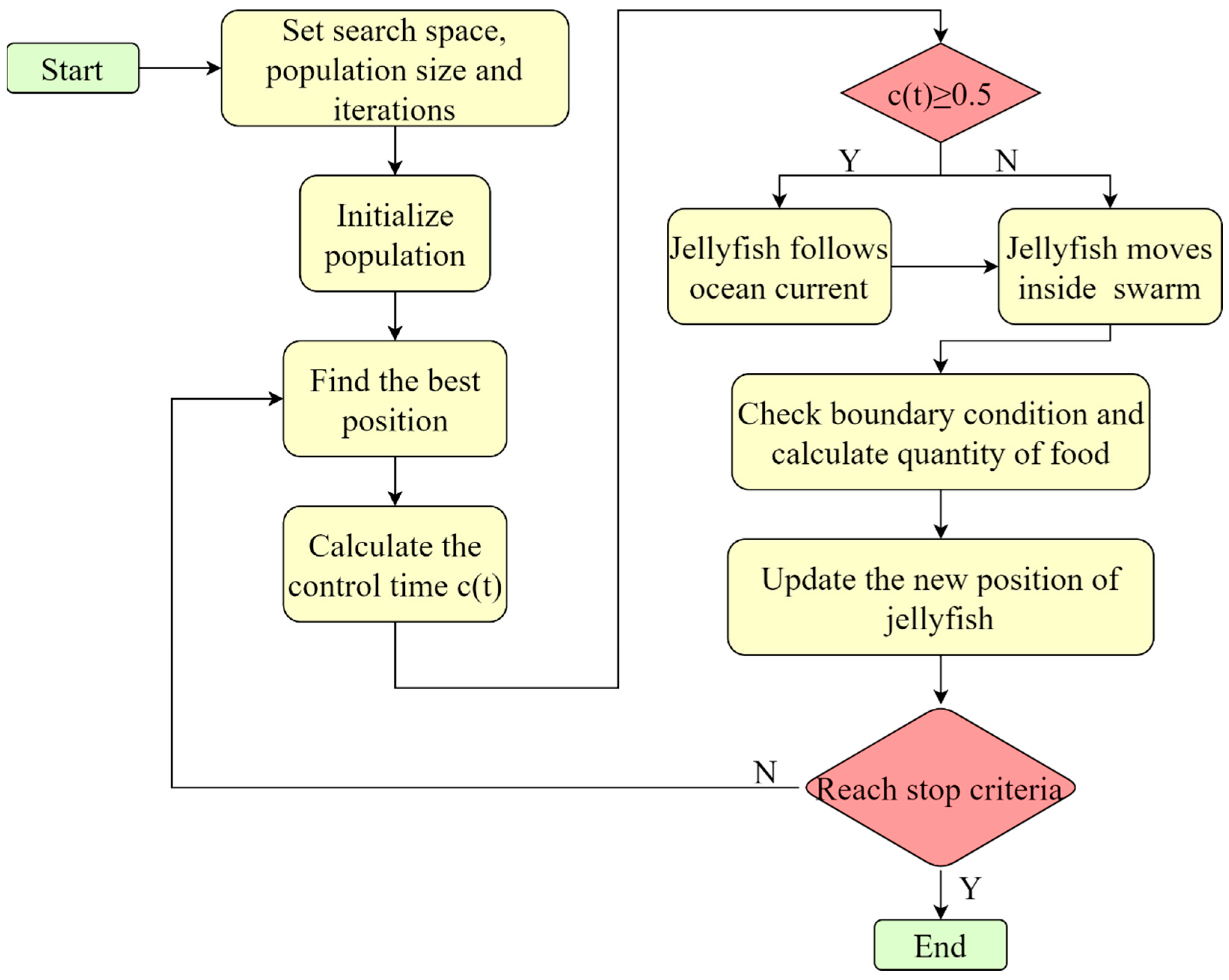
Chou and Truong [24] presented the Jellyfish Search Optimizer (JSO) derived from the predation and movement patterns of jellyfish populations. Jellyfish propel forward by expelling fluids from their bodies, even though water currents and tides are the primary factors influencing their motion [25]. When seeking food, jellyfish collectives will investigate potential foraging zones, assess the relative amount of food available, and then choose areas with the most advantageous characteristics. In this procedure, JSO employs the position of food to signify solutions in the space of domains. Some mathematical models used to describe the JSO optimization process are as follows [26].
(1) Population initialization
Due to the possibility of falling into local optima during random initialization, leading to slow convergence, JSO’s starting population is grounded in a chaotic mapping termed logical mapping, providing more varied initial populations. The mapping process is shown in the following equation:
x i + 1 = η x i ( 1 x i ) ,   0 x 0 1
Here, x i stands for the logistic chaotic value associated with the ith jellyfish and x 0 denotes the initial population of mappings. The range for x 0 is within (0, 1), excluding specific values like [0.0, 0.25, 0.5, 0.75, 1.0]. According to Chou and Truong [24], the parameter η is set at 4.0.
(2) Ocean current
Oceanic circulations, laden with a significant amount of nutrients, are apt to lure jellyfish toward their course. v trend represents the direction of ocean currents, reflecting the average position discrepancy between the best jellyfish and individual jellyfish in the population. The following equation is used to describe ocean currents:
v t r e n d = 1 N p i = 1 N P ( x * e c x i ) = x * e c u = x * β r a n d ( 0 , 1 ) μ
Here, N p denotes the jellyfish count, x * signifies their best position, e c stands for the attraction factor, with e c calculated as β·rand(0,1), μ denotes the average position of all jellyfish, and β is a constant set to 3 [24]. The term rand(0,1) represents a random value within the range of (0,1). Consequently, each jellyfish’s updated position is expressed in the following equation:
x i ( t + 1 ) = x i ( t ) + r a n d ( 0 , 1 ) · v t r e n d
(3) Jellyfish swarm time control mechanism
In the JSO algorithm, every jellyfish has two types of motion: passive and active [25]. Jellyfish employ passive motion to move independently without relying on information from their counterparts.
x i ( t + 1 ) = x i ( t ) + γ · r a n d ( 0 , 1 ) · ( U b L b )
Here, γ represents the motion coefficient, set at 0.1 [24], while   U b     and L b     denote the search space’s upper and lower bounds. Furthermore, jellyfish engage in active circular movements to discover other jellyfish. The following equation describes the process of this movement:
v d i r = x i ( t ) x j ( t )       i f   x i ( t ) > x j ( t ) x j ( t ) x t ( t )       i f   x i ( t ) < x j ( t )
x i ( t + 1 ) = x i ( t ) + r a n d ( 0 , 1 ) · v d i r
Here, v dir   signifies the dynamic motion of jellyfish while x j ( t ) indicates the position of a jellyfish (selected randomly), distinct from x i ( t ) .
(4) Boundary conditions
In the course of population initialization and iterative search, newly created jellyfish may revert to the opposite boundary when surpassing the limits of the boundary. This process can be described using the following equation:
x i , d = x i , d U b , d + L b , d   if   x i , d > U b , d x i , d L b , d + U b , d   if   x i , d < U b , d
Here, x i , d     indicates the position of the i th   jellyfish in the d th   dimension, and x i , d   represents the modified position of   x i , d . U b , d   and L b , d     signify the upper and lower bounds on the   d t h   dimension. The JSO flowchart is shown in Figure 4.

3. Data Preparation

3.1. Data Source

The data required for model training in this study is derived from the pull-out test database of 86 experiments by Bouteldja et al. [17].

3.2. Input Parameter Selection

The predictive model developed in this study utilizes seven input variables: ‘Test’, ‘Cable type’, ‘Medium’, ‘E’, ‘Length’, ‘w:c ratio’, and ‘Stress’. The output variable, or target, is the shear bond strength, denoted as ‘k’. Each variable is defined as follows: Test represents the location of pull-out test, Cable type represents the type of cable bolt, Medium represents the host medium of the cable bolt, E (GPa) represents Modulus of Elasticity, Stress (Mpa) represents the confining pressure, Length (m) represents the embedment length of the cable bolt, w:c ratio represents water–cement ratio, and k (MN/m/m) represents the shear bond strength.
The ‘Test’, ‘Cable type’, and ‘Medium’ features are non-numeric and therefore require conversion into a numerical format for model input. To accomplish this, one-hot encoding was employed using the get_dummies function from the Python v.2.3 Pandas library [27]. This method transforms a categorical feature with N distinct categories into N new binary features. For any given sample, only the binary feature corresponding to its original category will have a value of 1, while all others will be 0. For example, the ‘Test’ variable has two values, ‘field’ and ‘laboratory’. After processing with the get_dummies method, a certain data’s ‘Test’ variable will be decomposed into two variables, namely ‘Test_laboratory’ and ‘Test_field’. These variables are binary, with values of 0 and 1 representing absence and presence, respectively. Similarly, ‘Cable type’ will be decomposed into ‘Cable type_birdcage’, ‘Cable type_garford bulb’, ‘Cable type_nutcase’, ‘Cable type_standard’, and ‘Cable type_standard(twin)’; while Medium will be decomposed into ‘Medium_PVC’, ‘Medium_aluminum’, ‘Medium_concrete’, ‘Medium_granite’, ‘Medium_limestone’, ‘Medium_ryolite’, ‘Medium_schist’, ‘Medium_shale’, and ‘Medium_steel’.
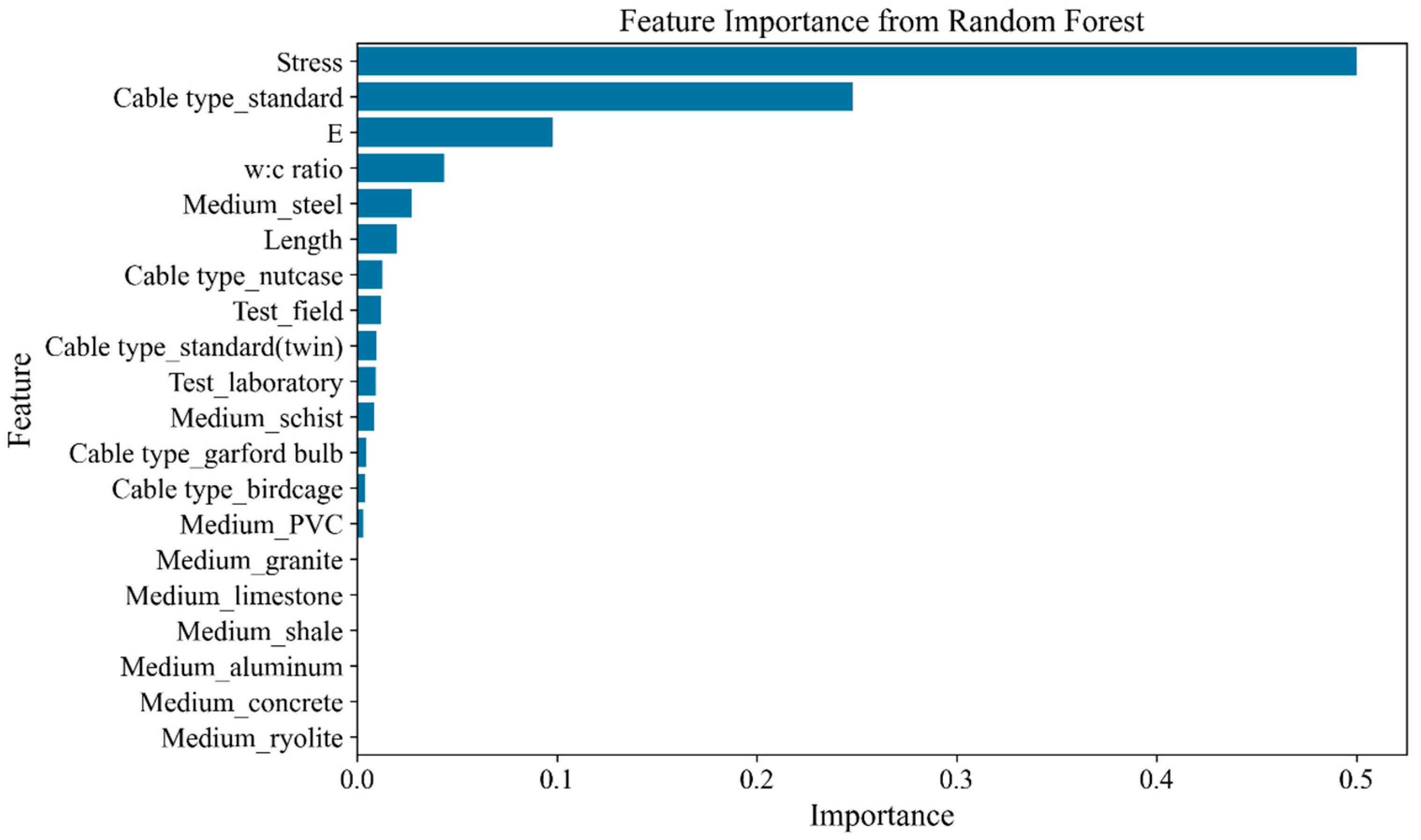
Due to the large number of variables, it is necessary to select the variables with the highest contribution. The selection process will be combined with a contribution analysis chart and a correlation analysis chart. Based on the contribution degree, the following input variables can be preliminarily selected from Figure 5: Stress, Cable type_standard, E, w:c ratio, Medium_steel, and Length.
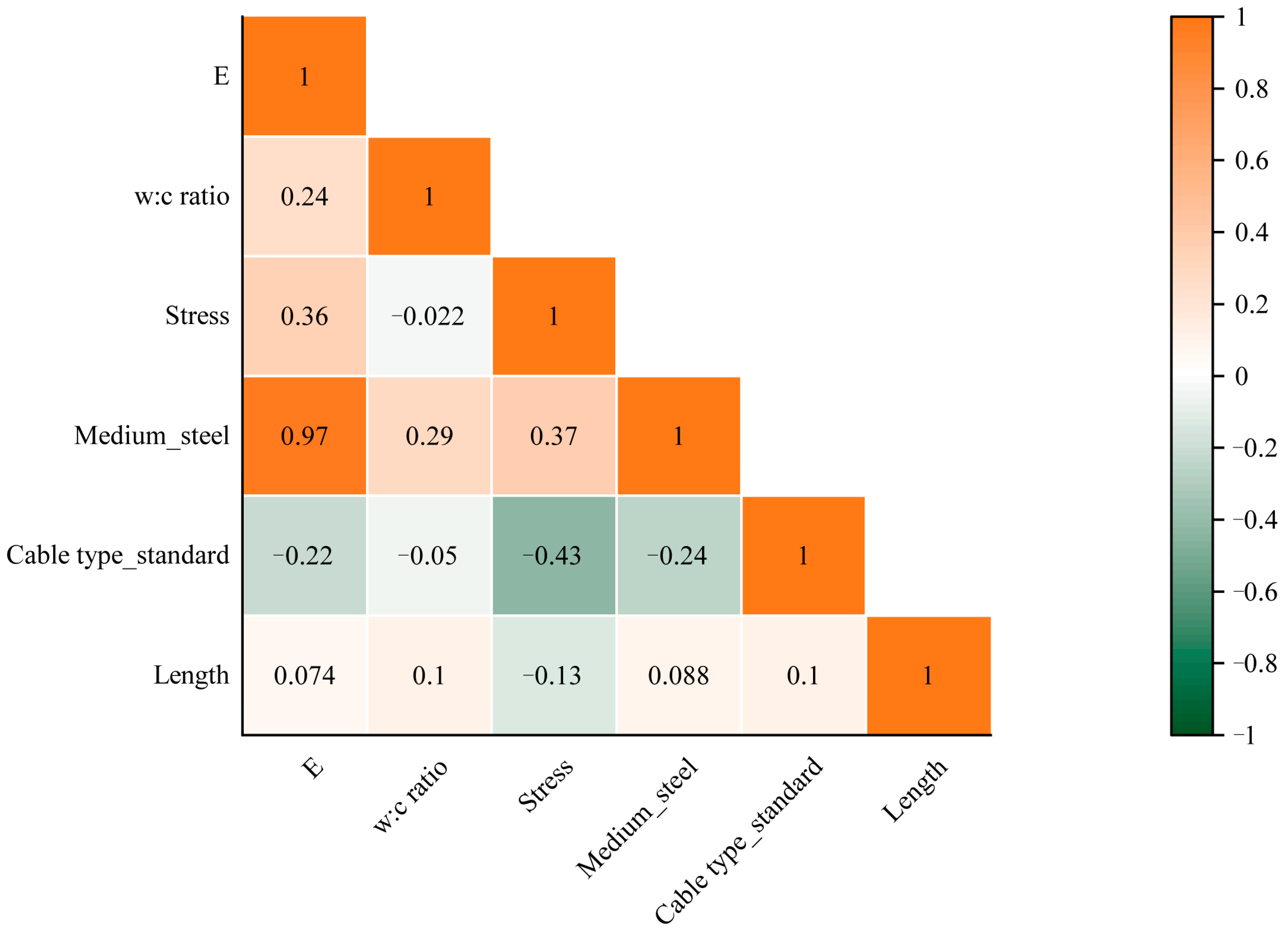
Figure 6 illustrates the correlation between input variables. Figure 6 shows that apart from the high correlation between E and Medium_steel, the correlations among other variables are relatively low. Due to the excessive correlation between E and Medium_steel, Medium_steel was excluded from the input variables. After selecting, the input variables of the model were ultimately determined as follows: Stress, Cable type_standard, E, w:c ratio, and Length.
To assess the potential for multicollinearity among the input variables, a Variance Inflation Factor (VIF) analysis was conducted. The VIF quantifies the extent to which a feature’s variance is inflated by its correlation with other features. The results of the analysis, presented in Table 1, show that all input features, ‘E’, ‘Length’, ‘w:c ratio’, ‘Stress’, and ‘Cable type_standard’, exhibited VIF values well below the commonly accepted threshold of 5.0. This indicates that multicollinearity is not a significant concern within the selected feature set, ensuring the stability and reliability of the subsequent model’s feature importance analysis.

3.3. Data Augmentation

Given that the performance and generalization capability of machine learning models typically improve with larger datasets, a data augmentation technique based on Gaussian noise was utilized to expand the original dataset. It is worth noting that the categorical variables processed by the ‘get_ dummies’ method do not require the addition of noise.
In this method, nine new, slightly perturbed instances were created for each of the 86 original samples. This was achieved by adding noise drawn from a normal (Gaussian) distribution to each feature of a sample. The noise distribution was specifically defined with a mean (µ) of 0 and a small variance of 0.03 (σ2).
A mean of 0 ensures that the noise is centered around the original value, meaning the augmentation process does not systematically increase or decrease the feature values on average, thus preserving the central tendency of the original data. The small variance of 0.03 was chosen to control the magnitude of the perturbations, ensuring that the synthetic data points remain physically and statistically representative of the original experimental conditions. The goal was to simulate minor, real-world measurement inaccuracies and material variability without introducing unrealistic samples that could distort the underlying physical relationships.
By repeating this process nine times for each original data point with independently generated noise, the dataset was expanded tenfold to 860 samples. This augmentation strategy serves a dual purpose: it increases the dataset size for more effective model training and enhances the model’s robustness by forcing it to learn the core patterns from a more diverse set of examples. Ultimately, this process is designed to improve the model’s ability to generalize its predictions to new, unseen data.

3.4. Data Distribution

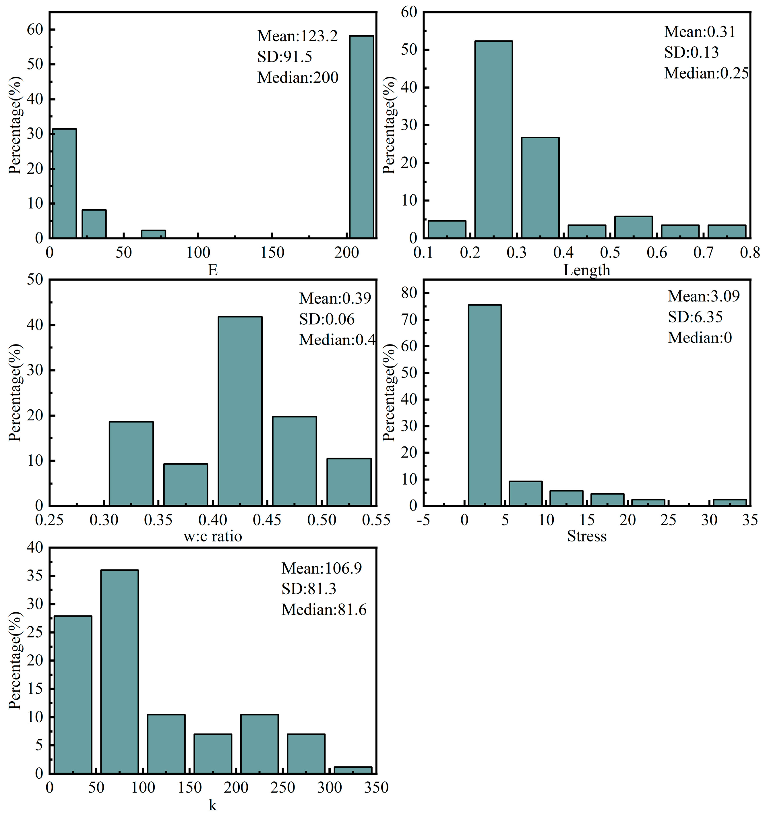
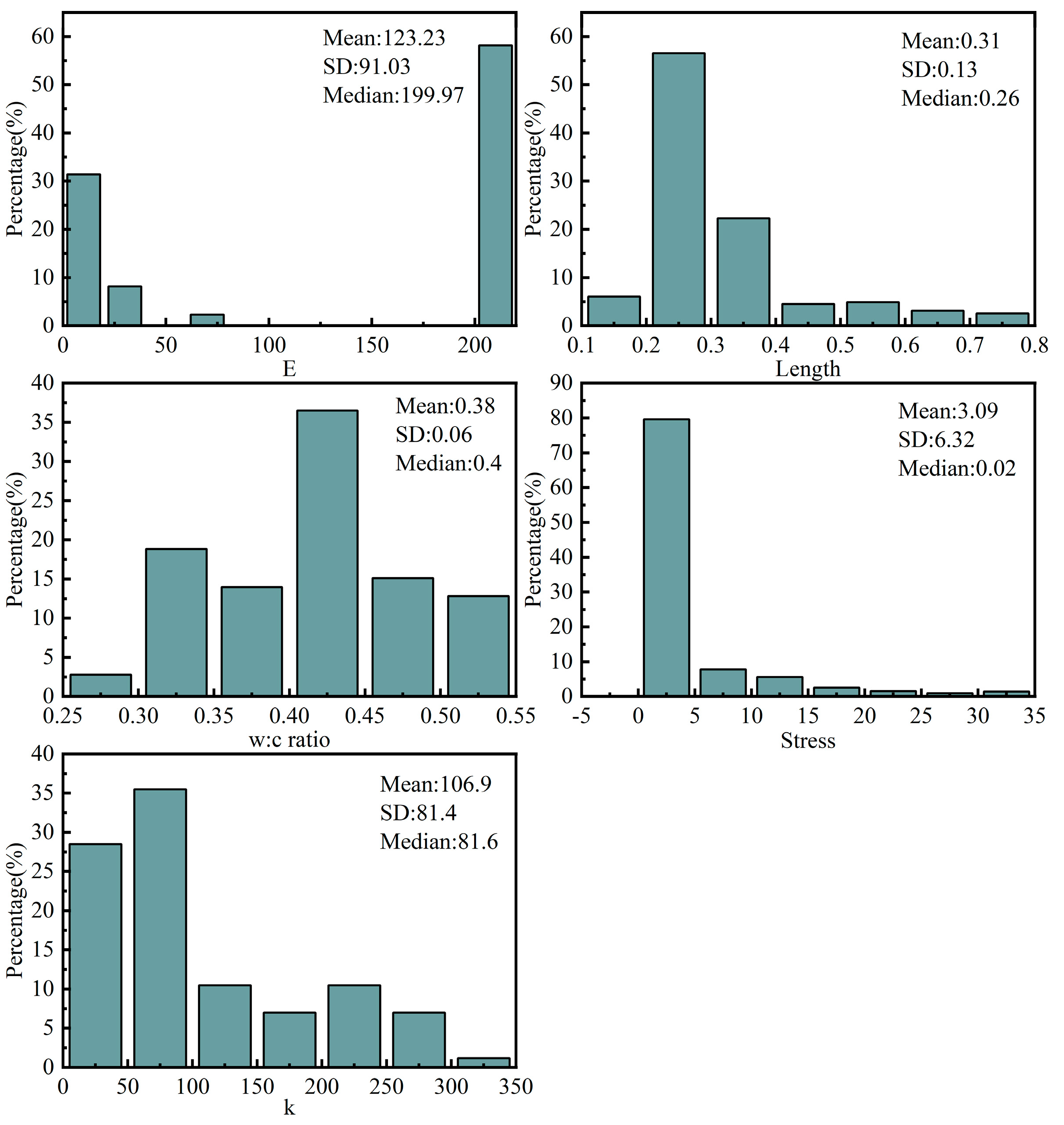
To further validate that the adopted noise-augmentation method, while expanding the dataset, did not significantly alter the inherent global distribution characteristics of the original data, a visual comparison of feature distributions before and after augmentation was conducted. Specifically, for numerical features, frequency histograms were plotted on both the original and augmented datasets, as illustrated in Figure 7 and Figure 8. Observation of these figures clearly shows that the feature histograms of the augmented dataset exhibit a high degree of similarity with the original dataset in terms of overall shape, central tendency (e.g., peak position), mean, standard deviation, and median, with no new unexpected patterns or significant systematic shifts attributable to the noise introduction being observed. As expected, due to the addition of zero-mean noise, the histograms of the augmented data display a slight and smooth broadening around the original peaks. This reflects a modest increase in variance and is a direct manifestation of generating new samples within the local neighborhood of the original data points, rather than a fundamental alteration of the distributional structure. Therefore, these comparative histograms visually corroborate the suitability of the selected noise level; it effectively increases data diversity while well preserving the core statistical distribution characteristics of the original data, thereby ensuring the effectiveness and reliability of training models based on this augmented data.

4. Model Development

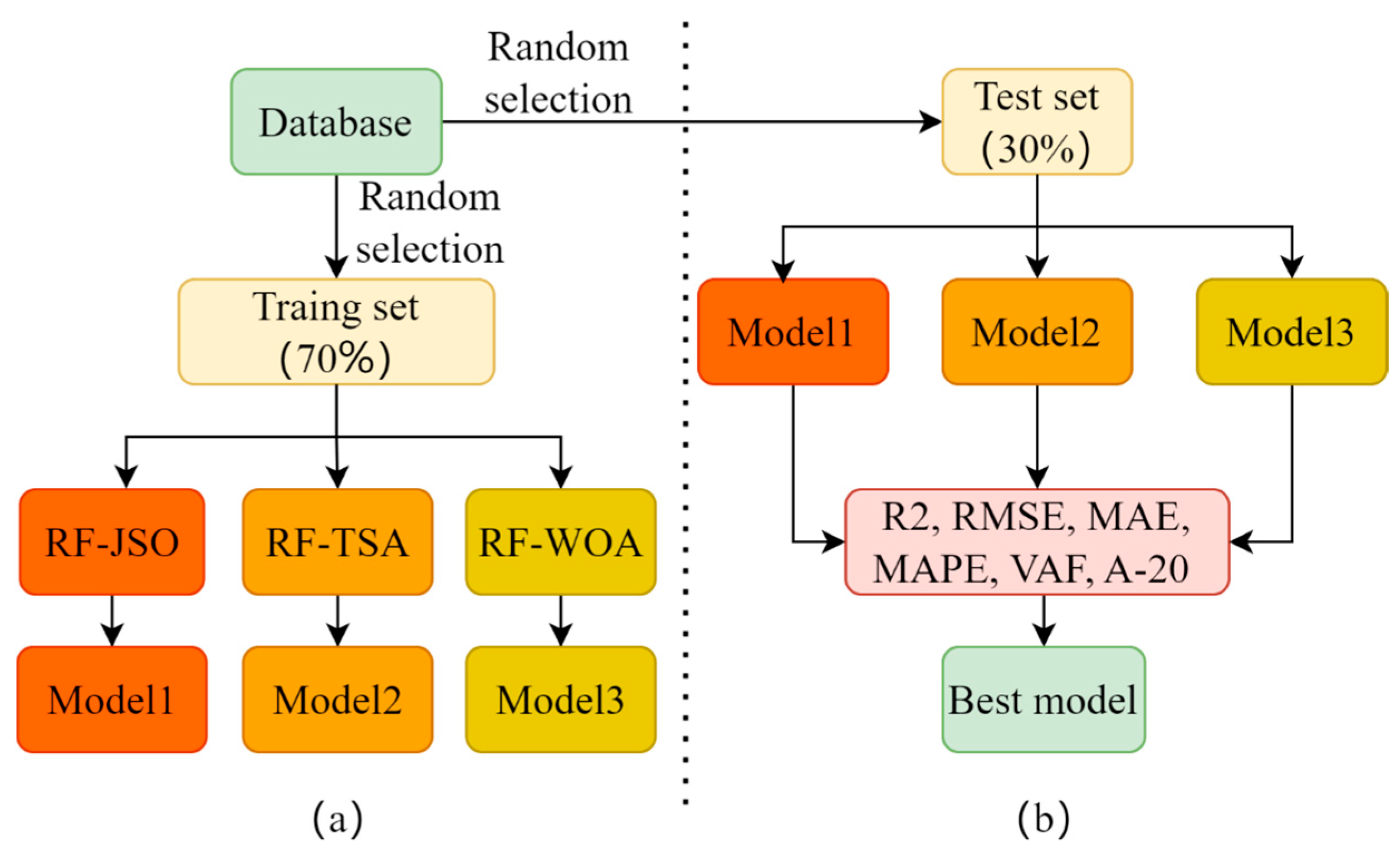
This study uses the aforementioned TSA, WOA, and JSO metaheuristic optimization algorithms to optimize the values of RF hyperparameters. The construction process of the model is shown in Figure 9. The random forest hyperparameters utilized in this study include n_estimators, max_depth, min_samples_split, min_samples_leaf, and max_features. Among them, n_estimators have the most significant impact on the predictive performance of RF. At the same time, the other four parameters are used to prevent the overfitting of RF by limiting the growth of branches and leaves.
Four RF-based models were created to compare the models’ performance, namely standard RF, RF-TSA, RF-WOA, and RF-JSO. Among them, ordinary RF uses default hyperparameters, while the remaining three hybrid models are used to find the optimal hyperparameters for RF. The process of establishing models is as follows:
(1) Prepare data
A new dataset containing 860 data points was constructed by generating random noise around each data point in the original database. A total of 70% of the database (602 data points) was used as the training set, and 30% (258 datapoints) was used as the testing set. The reason behind this ratio is rooted in the bias–variance trade-off. Allocating a substantial portion of the data (70%) for training is crucial for enabling the model to learn the underlying complex and nonlinear relationships within the data, thereby minimizing the risk of underfitting (high bias). Simultaneously, reserving a sufficiently large and independent portion of the data (30%) for testing ensures that the model’s generalization performance can be evaluated robustly and reliably. A smaller test set might lead to a noisy and statistically insignificant evaluation, while a smaller training set could compromise the model’s learning capacity. Therefore, the 70/30 split is considered to provide a reasonable balance between providing enough data for model training and retaining enough data for a meaningful performance validation [28,29,30].
(2) Set parameters
The range of n_estimators, max_depth, min_samples_split, min_samples_leaf, and max_features is set to [50, 400], [1, 20], [2, 50], [1, 50], and [1, 50], respectively. As for the optimization algorithm, the population is set to 50, and the number of iterations is set to 100.
(3) Hyperparameter update
When optimizing the algorithm, the fitness value is calculated generation by generation and gradually compared to find the optimal solution (hyperparameter). At the end of the run, the hyperparameter corresponding to the minimum fitness value is the optimal hyperparameter.
The hybrid model uses mean square error (MSE) as the fitness function that the metaheuristic algorithm needs to solve. The representation of mean square error is shown in the following equation:
M S E = 1 n i = 1 n ( Y i Y ^ i ) 2
To ensure the robustness of the optimization process and prevent overfitting, five-fold cross-validation was applied during the evaluation of each candidate solution’s fitness. For each set of hyperparameters proposed by the metaheuristic algorithms, the average MSE across the five folds was computed and used as the fitness value. This approach ensures that the selected hyperparameters generalize well across different data splits. Additionally, after obtaining the optimal hyperparameters for each model, the final models were retrained on the entire training set and evaluated on the test set to further validate their generalization performance.
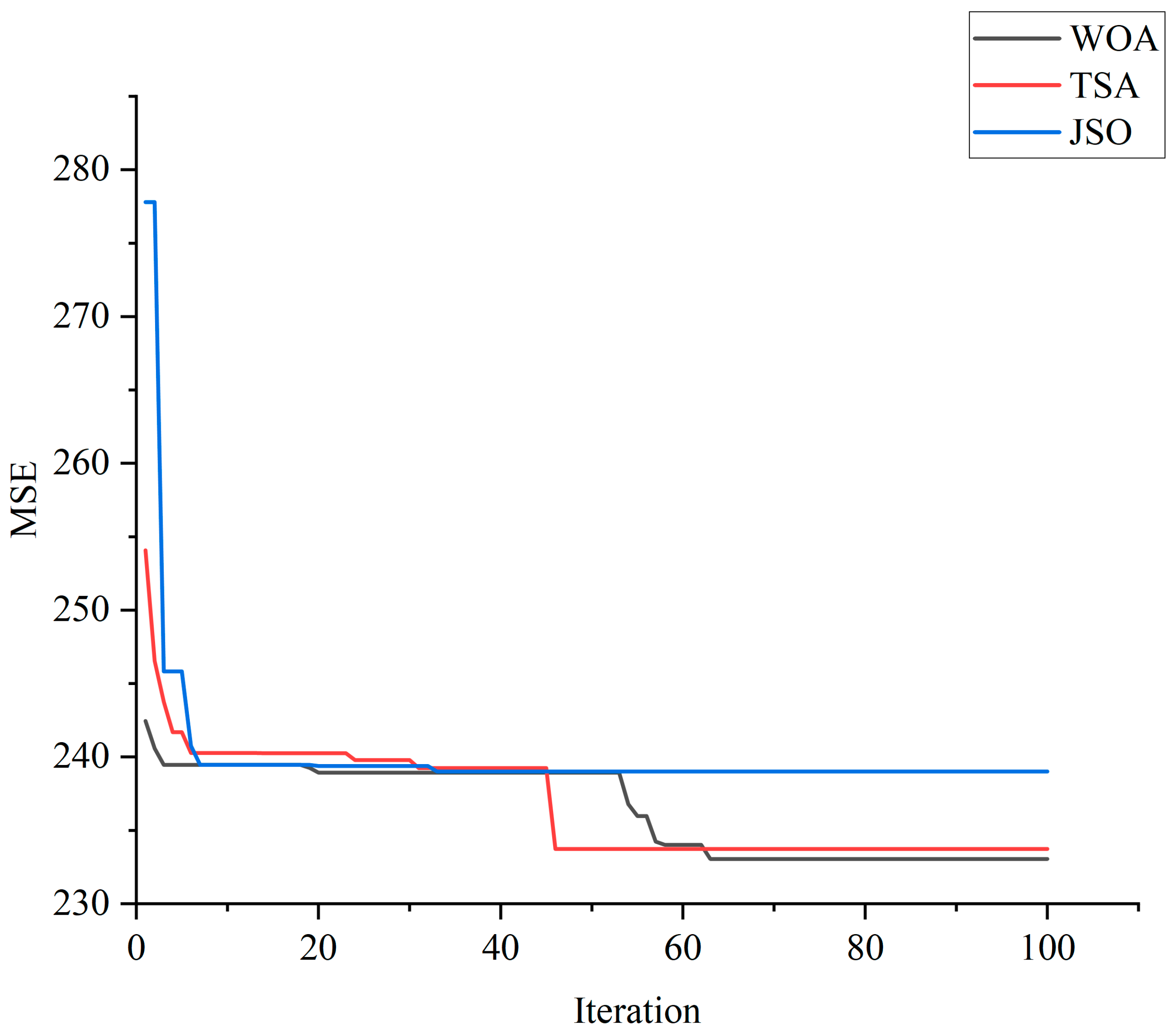
Figure 10 shows that the JSO algorithm exhibits the fastest initial convergence speed, converging to an MSE value of approximately 239 after about 35 iterations. The TSA algorithm found the final optimal solution at around the 45th iteration, with an MSE value of about 233. The WOA algorithm, after converging to a suboptimal plateau in the early stage, successfully escaped it around the 50th iteration and finally converged near the 65th iteration to an optimal MSE value similar to that of TSA. Although WOA achieves the smallest optimized MSE value, it does not guarantee optimal hyperparameters. Further model evaluation is necessary for obtaining optimal hyperparameters. In the following text, six indicators (R2, RMSE, MAE, MAPE, VAF, and A-20 index) will be used to evaluate each model specifically.
Table 2 shows the hyperparameters obtained for each hybrid model. Compared to the default RF, all three hybrid models use an approximate and slightly smaller number of decision trees. In addition, all hybrid models have trimmed the branches and leaves of RF to reduce the occurrence of overfitting. It should be emphasized that the hyperparameters in the table are obtained through the training set.

5. Results and Discussion

5.1. Selecting the Best Model

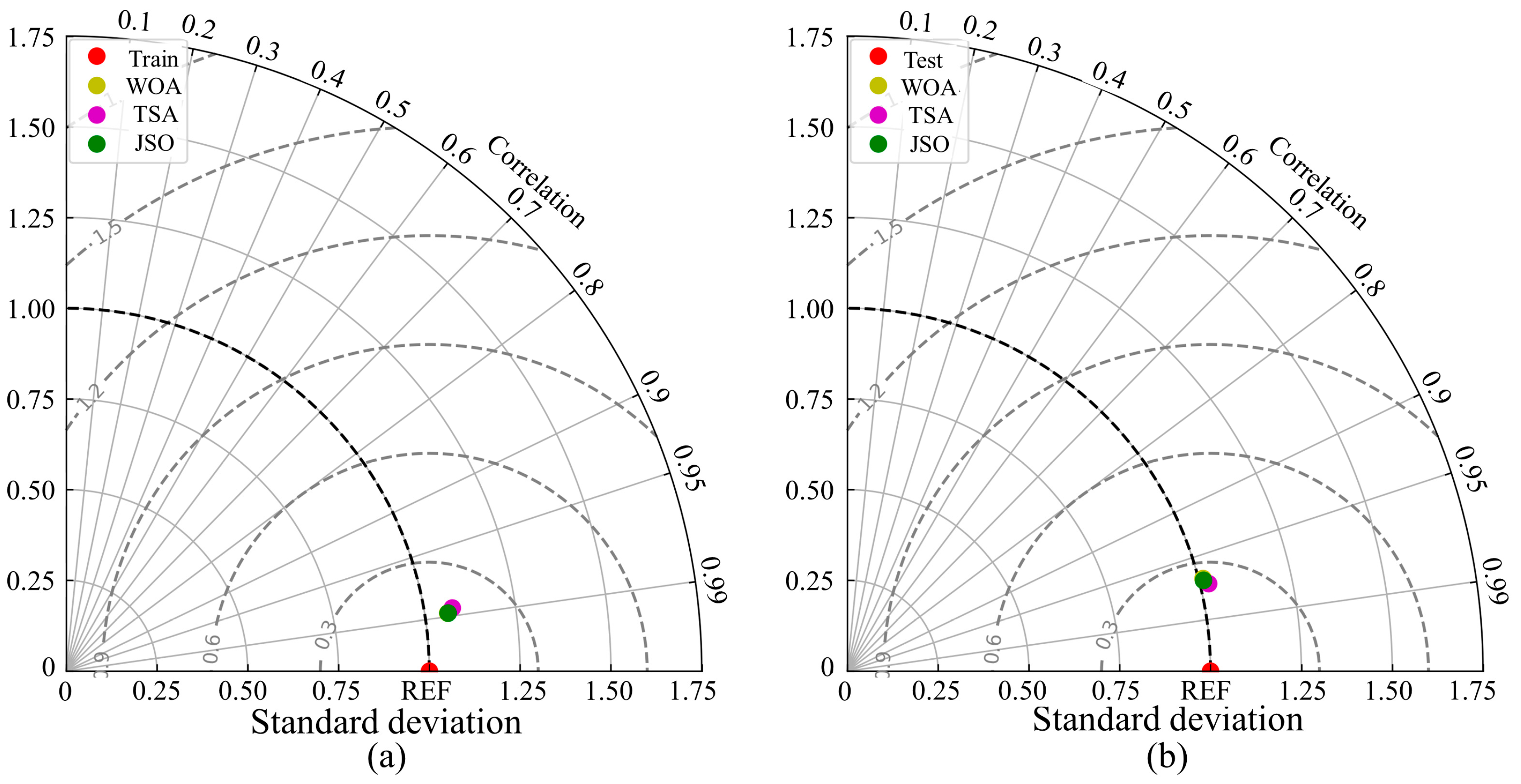
In order to select the optimal model, each model made predictions on both the training and testing sets, and then the most precise model was chosen based on its performance. The Taylor diagram, as a tool for visualization, has the ability to show the differences between model predictions and actual results [31]. These differences can be subsequently measured using indicators such as correlation coefficient (R2), standard deviation (SD), and centered root mean square error (cRMSE).
Figure 11 illustrates the differences between the predicted values of each model and the actual values (i.e., “REF”), where proximity to the ‘REF’ point on the horizontal axis indicates a better fit. This is achieved through a three-way relationship between the plotted points and the graphical axes. The standard deviation of each model is represented by its radial distance from the origin (0,0). The dashed black arc that passes through the ‘REF’ point specifically indicates the standard deviation of the actual observations, serving as a benchmark for variance. The correlation coefficient is given by the azimuthal angle, with values marked on the outer curved axis. The gray radial lines extending from the origin are lines of constant correlation, allowing for a quick assessment of how well the model’s pattern matches the observations. Finally, the centered root mean squared error (cRMSE) between a model and the reference data is proportional to the distance from the ‘REF’ point. The dashed gray arcs centered on ‘REF’ are contours of equal cRMSE, providing a direct visual measure of the model’s error magnitude. As illustrated in the figure, the performance of the three hybrid models on the training set and the test set is very close, making it difficult to determine which model performs best. Therefore, a more precise method is needed to find the best-performing model.
To quantify the predictive performance of the model, this study used the following six criteria for evaluation: coefficient of determination (R2), root mean squared error (RMSE), mean absolute error (MAE), mean absolute percentage error (MAPE), variance accounted for (VAF), and A-20 index [4]. R2 represents the degree of correlation between the predicted and actual values, with a range of values between 0 and 1. The closer to 1, the better; RMSE indicates the square root of the average square difference between the predicted and actual values, with values closer to 0 being better; MAE signifies the average absolute error between the predicted value and the actual value, and the closer it is to 0, the better; MAPE denotes the average absolute value of the relative error between the predicted value and the actual value, usually expressed as a percentage, and the closer it is to 0, the better; VAF measures model capability by comparing the standard deviation of errors with the standard deviation of actual values, with values ranging from 0 to 1, and the closer to 1, the better; and the A-20 index represents the proportion of cases where the absolute difference between predicted and actual values is less than or equal to 20% of the actual value, with values ranging from 0 to 1, and the closer to 1, the better. Each of the chosen metrics evaluates the model’s performance from a different perspective, and their joint consideration ensures a more holistic and reliable assessment. Metrics like R2 and VAF assess the goodness-of-fit and the proportion of variance explained by the model, providing an overall sense of its explanatory power. Error-magnitude metrics such as RMSE and MAE quantify the average absolute prediction error. RMSE is particularly sensitive to large errors (outliers) due to the squaring term, while MAE provides a more direct measure of the average error magnitude. Relative error metrics like MAPE evaluate the prediction error relative to the actual value, which is crucial for understanding the model’s performance across different scales of the target variable. Finally, the A-20 index, a domain-specific metric, provides a practical measure of reliability by calculating the percentage of predictions that fall within an acceptable engineering tolerance (±20%). By evaluating the models against this diverse set of criteria, a more nuanced and trustworthy conclusion regarding the overall best-performing model can be drawn, mitigating the potential biases of any single metric.
The mathematical expressions for the above standards are as follows [1]:
R 2 = 1 i = 1 n ( y i y ^ i ) 2 i = 1 n ( y i y ¯ i ) 2
R M S E = 1 n i = 1 n ( y i y ^ i ) 2
M A E = 1 n i = 1 n y i y ^ i
M A P E = 1 n i = 1 n y i y ^ i y i
V A F = ( 1 var ( y i y ^ i ) 2 var ( y i ) ) × 100 %
A 20 = m 20 n
Here, y i   represents the actual value, y ^ i   represents the predicted value, y ¯ i   represents the average of the actual values, n represents the total number of samples, var(x) represents the variance of x, and m20 represents the number of samples where the ratio of the smaller number to the larger number between the actual and predicted values lies within the range of 0.8 to 1.
For the evaluation of the model’s predictive ability, the method proposed by Zorlu et al. [32] was adopted. This method provides a quantitative framework to rank the models based on their collective performance across all evaluation metrics. For each of the six metrics (R2, RMSE, MAE, MAPE, VAF, and A-20), the four models (standard RF and the three hybrid models) were ranked separately for the training set and the testing set. A point-based system was used for ranking. The best-performing model for a given metric received a score of 4, the second-best received a score of 3, the third-best received a 2, and the lowest-performing model received a score of 1. The final score for each model was then calculated as a weighted sum of its scores across all metrics and both stages. To emphasize the model’s generalization ability, the scores from the training set were assigned a weight of 30%, while scores from the testing set were given a higher weight of 70%.
Table 3 shows the scores of the initial RF and three hybrid models on the training set and testing set. Among them, RF-JSO (18.3) scored the highest, followed by RF-WOA (17.3) and RF-TSA (15.3), and the initial RF (13.5) scored the lowest. Therefore, these results lead to the conclusion that the best-performing model is the RF-JSO model with n_estimators = 213, max_depth = 9, min_samples_leaf = 3, min_samples_split = 2, and max_features = 6. The use of five-fold cross-validation during the optimization process ensures the validity of the obtained hyperparameters and enhances the reliability of the final model performance reported in Table 3.
Figure 12 presents a visual comparison of the models’ generalization performance across three key metrics. The results clearly demonstrate the effectiveness of the hyperparameter optimization process. In all three metrics, the hybrid models (RF-JSO, RF-TSA, RF-WOA) consistently outperform the standard RF model. Specifically, the RF-JSO model exhibits the highest R2 (0.981) and the lowest RMSE (11.063) and MAE (6.46), confirming its superior predictive accuracy and reliability among all evaluated models. This graphical representation visually corroborates the quantitative findings in Table 3, highlighting the tangible performance gains achieved through systematic optimization.
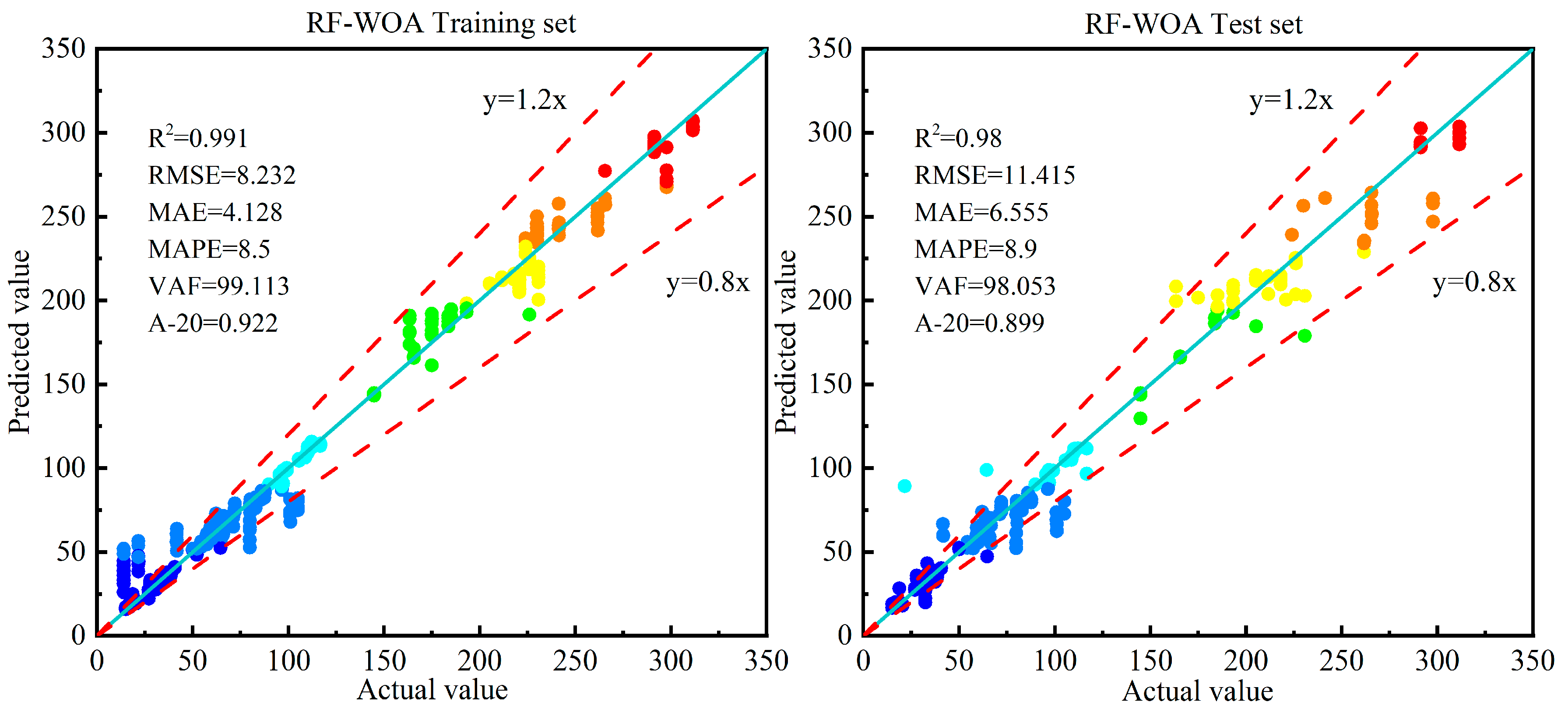
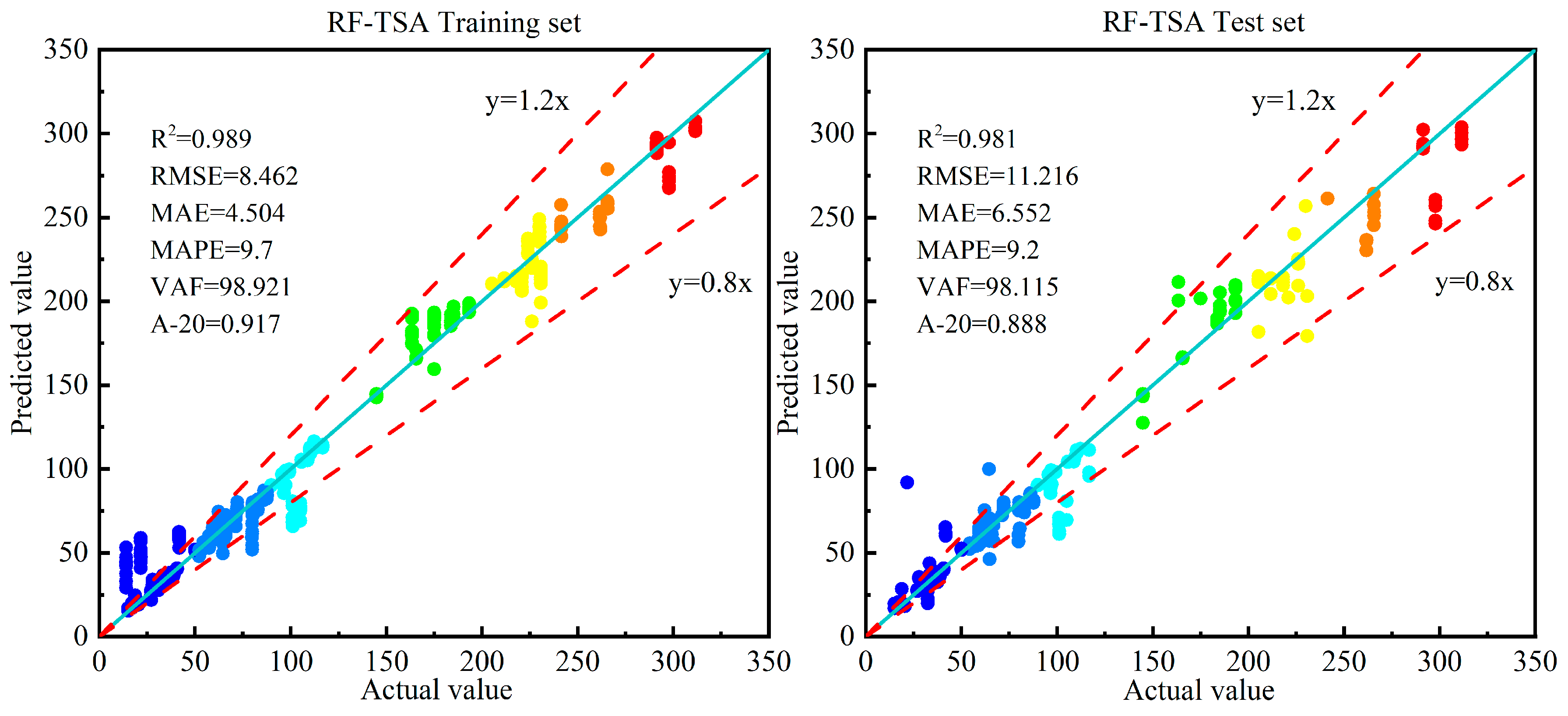
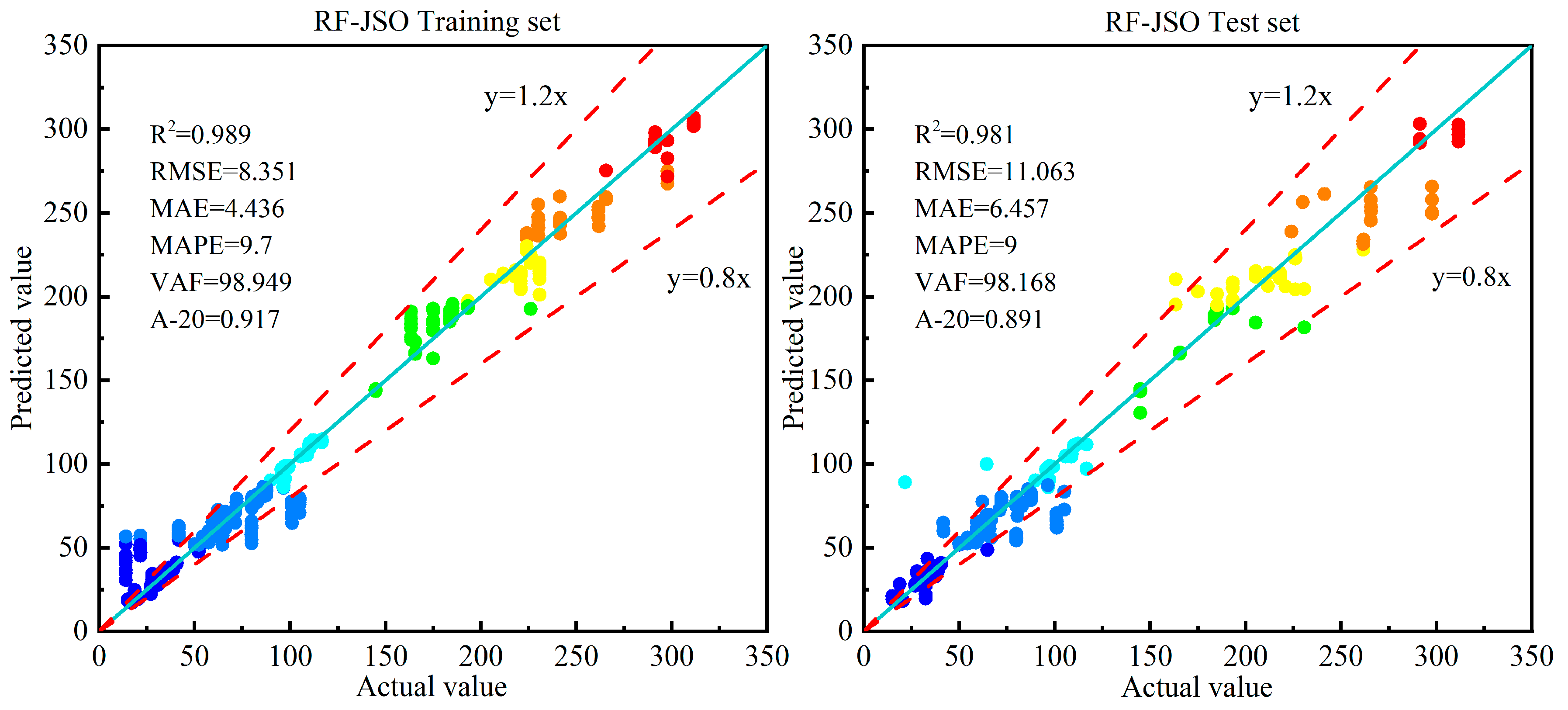
In addition, the visualization of model prediction performance is also essential. Figure 13, Figure 14 and Figure 15 compare the predicted and actual values of RF-JSO, RF-WOA, and RF-TSA on the training and testing sets. In these plots, the solid cyan line (y = x) represents a perfect prediction, where the predicted value exactly equals the actual value. The two dashed red lines represent the ±20% error bounds (y = 1.2x and y = 0.8x), providing a visual reference for the A-20 index; points falling between these lines have a relative error of less than 20%. The data points are colored according to their value to indicate data density along the performance line. From these figures, all three hybrid models achieve an excellent fit on the training sets, with data points tightly clustered around the perfect prediction line. More importantly, this high level of accuracy is maintained on the test sets, where the points remain closely distributed around the y = x line and largely within the ±20% error bounds. This demonstrates that the models possess strong generalization capabilities and are not overfit. While all models perform exceptionally well, a subtle visual comparison of the test set plots indicates that the RF-JSO model shows the tightest data point clustering, particularly in the higher value range. This visual evidence supports the quantitative metrics that identify RF-JSO as the most accurate and robust model among the three.
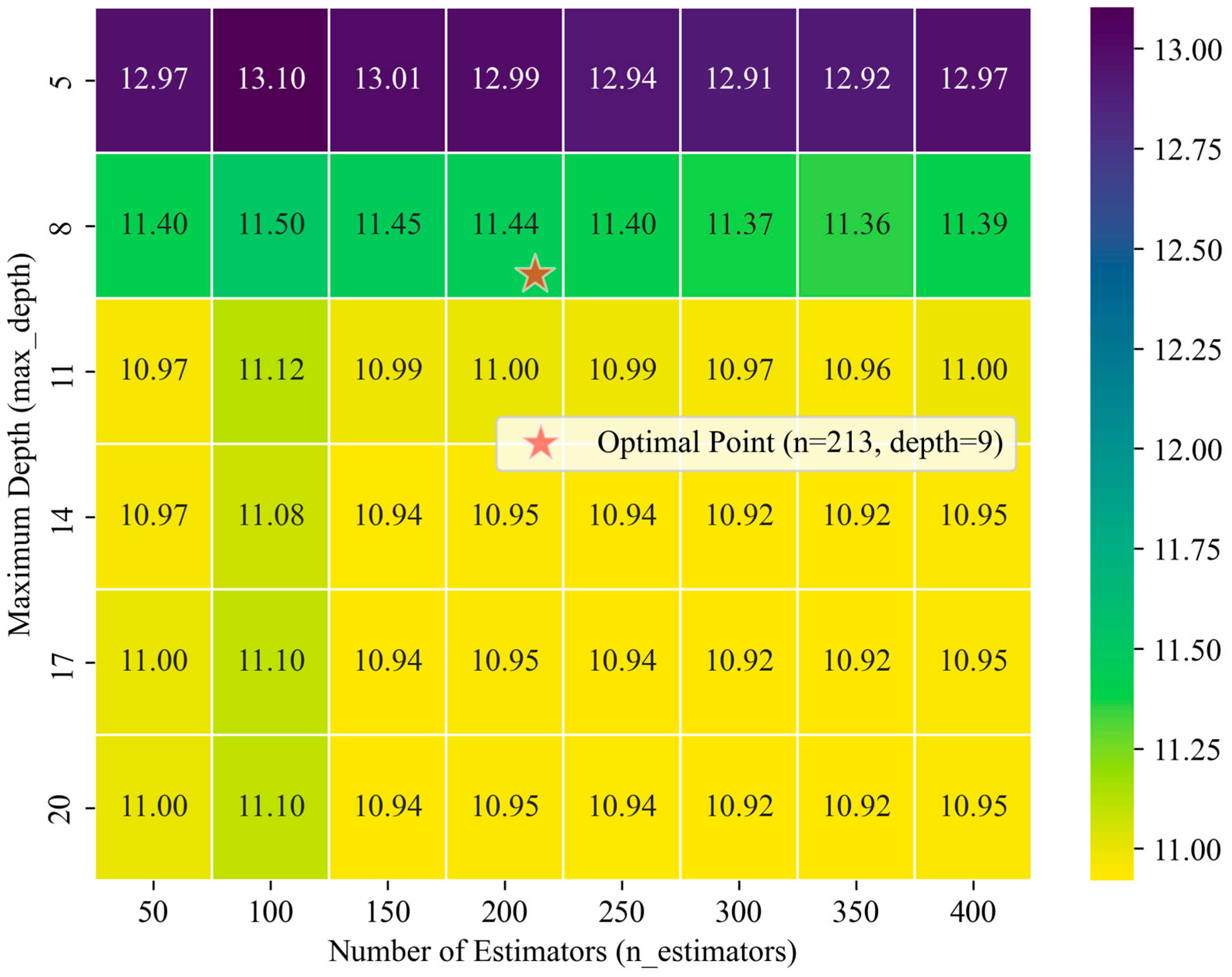
To provide a deeper insight into the optimization process and to evaluate the model’s sensitivity to its key hyperparameters, a comprehensive sensitivity analysis was conducted. The joint influence of the two most critical hyperparameters, n_estimators and max_depth, on the model’s predictive performance was investigated. The test set RMSE was calculated across a grid of n_estimators (from 50 to 400) and max_depth (from 5 to 20) values. The results are visualized as a heatmap in Figure 16. The heatmap offers several key insights. Firstly, it functions as a robust sensitivity analysis. A clear performance gradient is visible; along the vertical axis (max_depth), the model is highly sensitive to changes at lower depths. For example, increasing max_depth from 5 to 8 results in a significant drop in RMSE from ~13.0 to ~11.4, indicating that a shallow depth leads to an underfitting model. However, increasing the depth beyond 11 yields only marginal improvements, suggesting the model performance has begun to plateau. Along the horizontal axis (n_estimators), a similar pattern of diminishing returns is observed. For any given depth, increasing the number of estimators generally improves performance up to a point (around 150–200), after which the RMSE becomes very stable.
Secondly, and most importantly, the analysis serves as a practical convergence diagnostic for our optimization algorithm. The optimal point identified by the JSO algorithm (n_estimators = 213, max_depth = 9), marked by a red star, is located squarely within the high-performance region (the transition from green to bright yellow). It successfully avoided the underfitting zone (dark purple) while also not selecting an overly complex model (e.g., max_depth = 20) where performance gains are negligible. This provides strong validation that the JSO optimization process effectively converged to a robust and genuinely high-performing solution within the parameter space.
To highlight the performance of the models developed in this study, two interpretable benchmark models were introduced for comparison: XGBoost and LGBM. XGBoost is an efficient gradient-boosting tree algorithm that demonstrates strong fitting capabilities and generalization performance when processing structured data, through optimizations such as regularization, pruning, and block caching. LightGBM is a gradient boosting framework that employs a histogram-based decision tree learning strategy and a leaf-wise growth approach, resulting in faster training speeds and lower memory usage, making it particularly suitable for large-scale data modeling. The comprehensive performance comparison is presented in Table 4. While all three models demonstrate strong performance on the training set, the evaluation on the test set is crucial for assessing their true generalization capabilities. On the test set, the proposed RF-JSO model achieved a higher R2 (0.981) and a significantly lower RMSE (11.063) compared to both XGBoost (R2 of 0.971, RMSE of 13.617) and LGBM (R2 of 0.9676, RMSE of 14.593). This pattern of superior performance is consistent across all other evaluation metrics. The RF-JSO model also recorded lower error values for MAE (6.457) and MAPE (9) and higher scores for VAF (98.1) and the A-20 index (0.891). These results conclusively demonstrate that for this specific application, the proposed RF-JSO model performs better than the benchmark models in both accuracy and reliability.

5.2. Model Interpretation

5.2.1. Importance Analysis of Input Variables

This section will employ the contribution analysis method for each input variable to interpret the model, aiming to understand the weight of each parameter in the prediction process, identify key input parameters affecting prediction performance, and enhance model interpretation. The RF-JSO model, identified as the best in the previous text, will be analyzed using methods like Shapley Additive exPlanations (SHAP), Partial Dependence Plot (PDP), and Local Interpretable Model-agnostic Explanations (LIME) [27,33,34,35,36,37,38,39] to assess input variable contributions and improve understanding of its behavior.
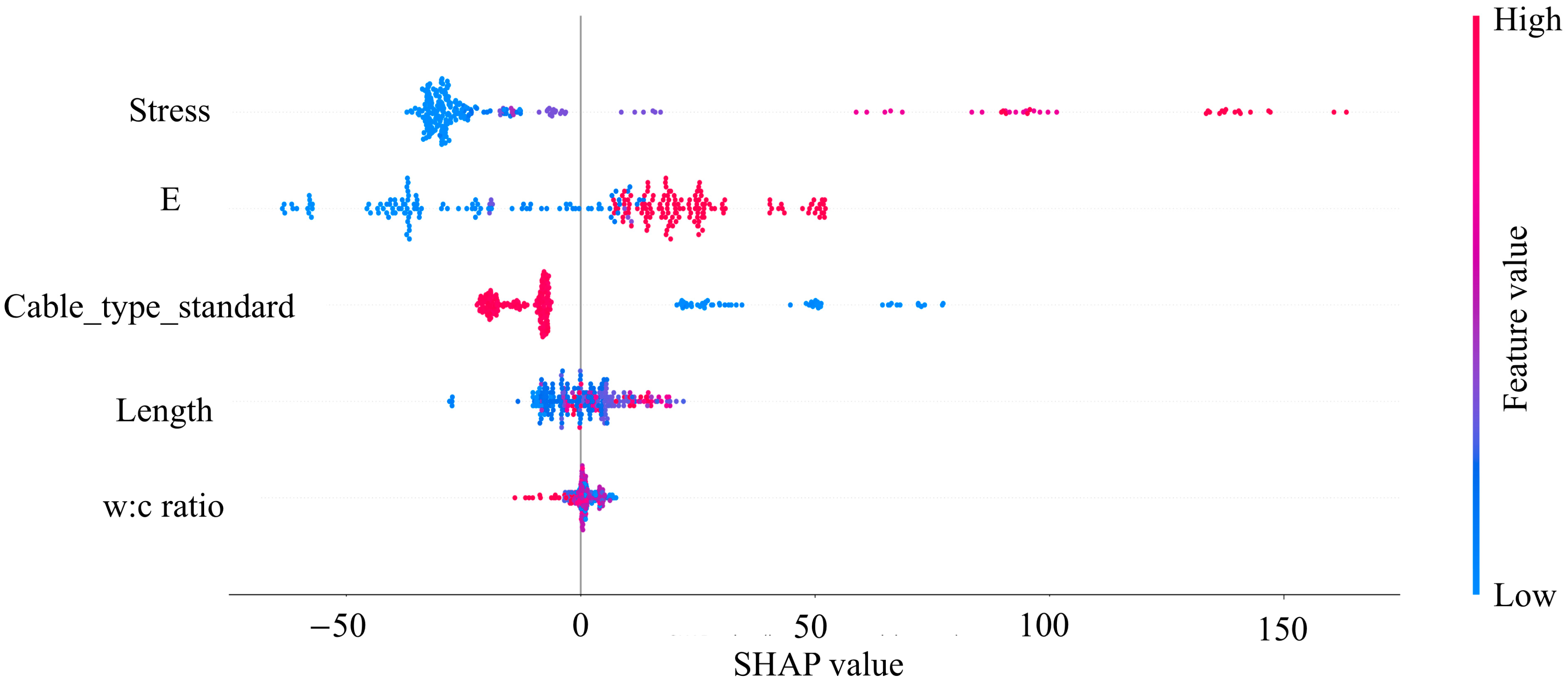
Figure 17 is a SHAP beeswarm graph, which provides the influence and contribution of each feature on the model’s prediction results based on the Shapley values of each feature. Each point on the graph represents a sample, with feature value sizes indicated by point colors; red denotes high values, and blue denotes low values. The x-axis illustrates the SHAP value, reflecting the feature’s impact on predictions. Positive values indicate promotion of prediction, while negative values indicate suppression of prediction. Greater absolute SHAP values signify a more substantial impact on the prediction results.
Figure 17 shows that stress, E, Cable type_standard, Length, and w:c ratio are the five variables influencing the model’s shear bond strength prediction. From the figure, it is evident that stress has the greatest influence on the model’s predictions, followed by E. Both exhibit the same pattern; lower values lead to lower predicted values, and higher values lead to higher predicted values. For Cable type_standard, the figure clearly illustrates that the model tends to produce lower predicted values when the cable type is standard. Length and w:c ratio have much smaller impacts on the model. Larger Length values cause the model to predict higher values, whereas smaller Length values result in lower predictions. The w:c ratio affects the model oppositely to Length.
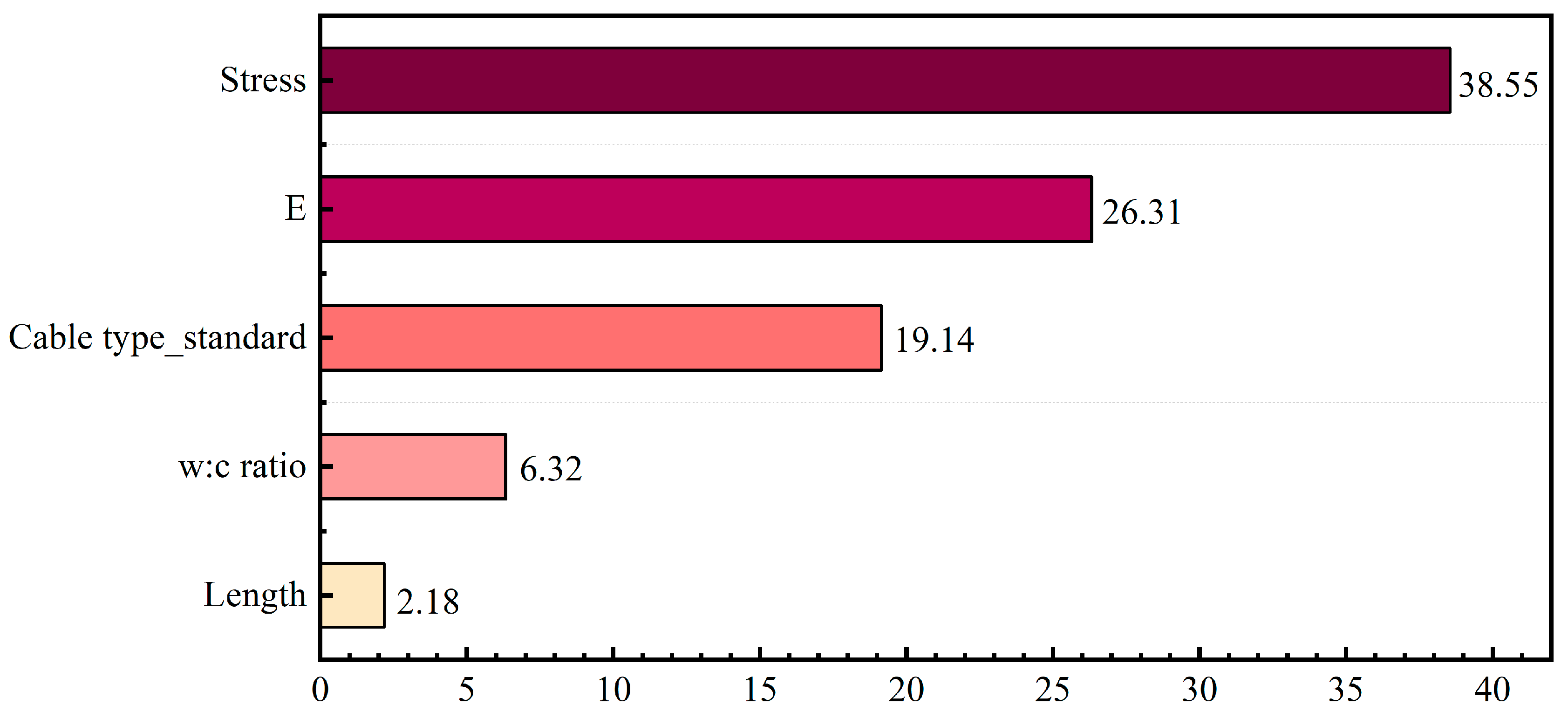
To provide a more precise and quantitative illustration of each input variable’s influence on the model’s predictions, a SHAP global feature importance plot is presented in Figure 18. This plot ranks the features based on the mean absolute SHAP value across all samples in the dataset. A higher mean absolute SHAP value signifies a greater overall impact on the model’s output. The results clearly indicate a hierarchical structure in feature importance. ‘Stress’ (confining pressure) emerges as the single most influential predictor, with a mean SHAP value of +38.55, suggesting it has a substantially larger impact on the model’s predictions than any other variable. Following ‘Stress’, a second tier of important features is formed by ‘E’ (elastic modulus) and ‘Cable_type_standard’, with mean SHAP values of 26.31 and 19.14, respectively. Though not as dominant as ‘Stress’, these two features still exert considerable influence on the model’s output. The remaining two features, ‘Length’ and ‘w:c ratio’, form a third tier with much smaller SHAP values (6.32 and 2.18). This demonstrates that while they do contribute to the prediction, their overall impact is significantly less pronounced compared to the other three variables.

5.2.2. Analysis of the Impact of Changes in Input Variables

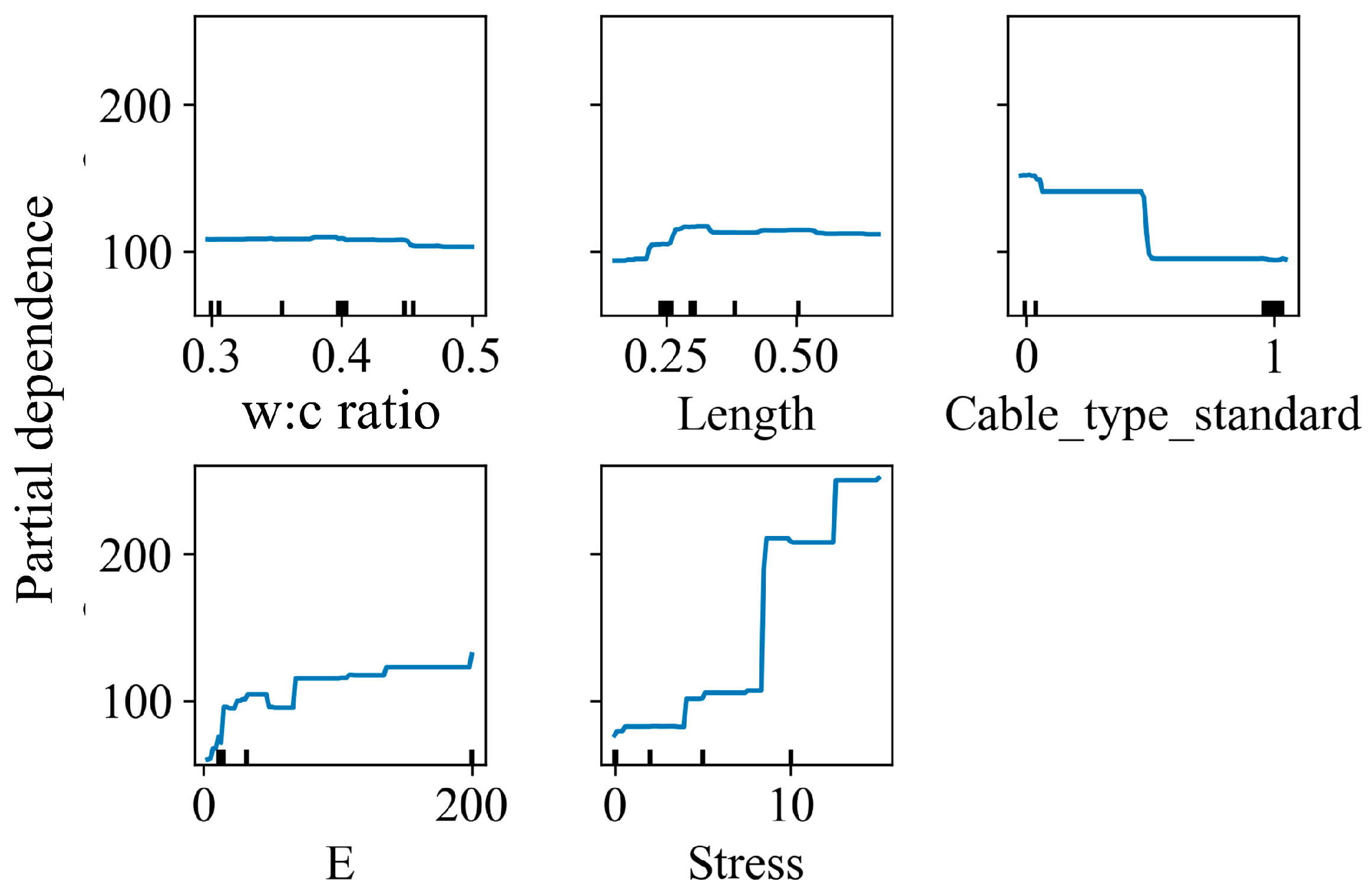
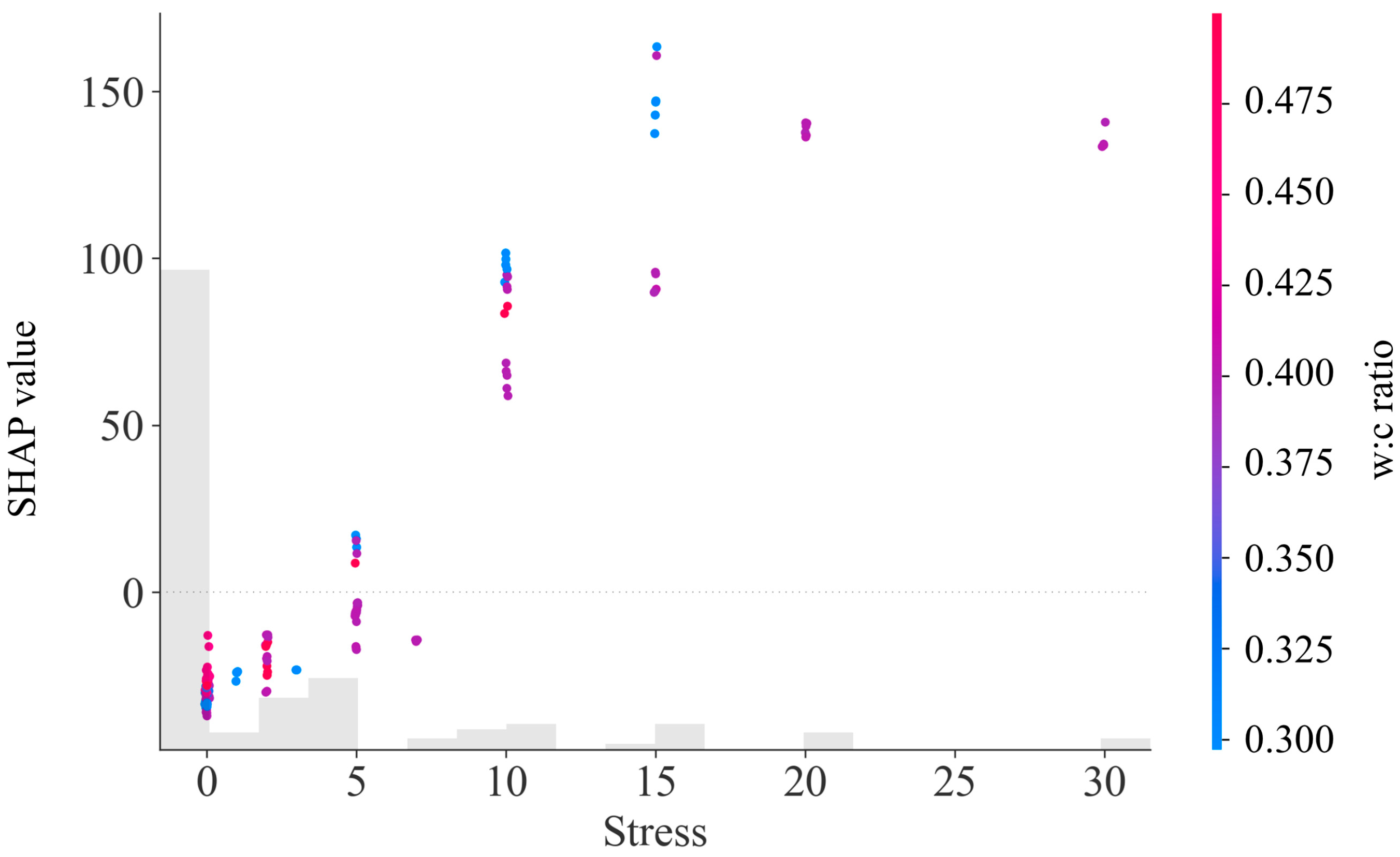
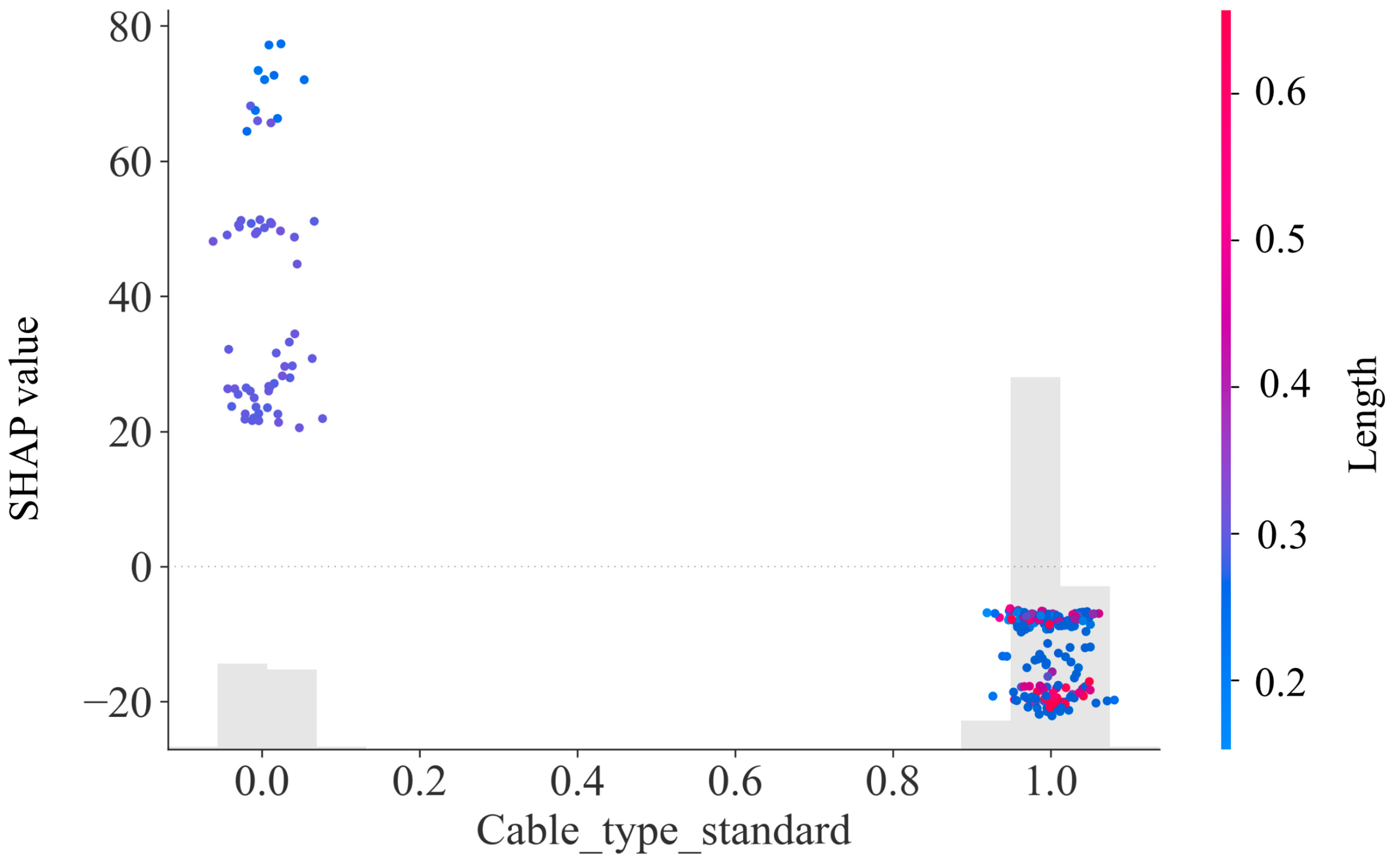
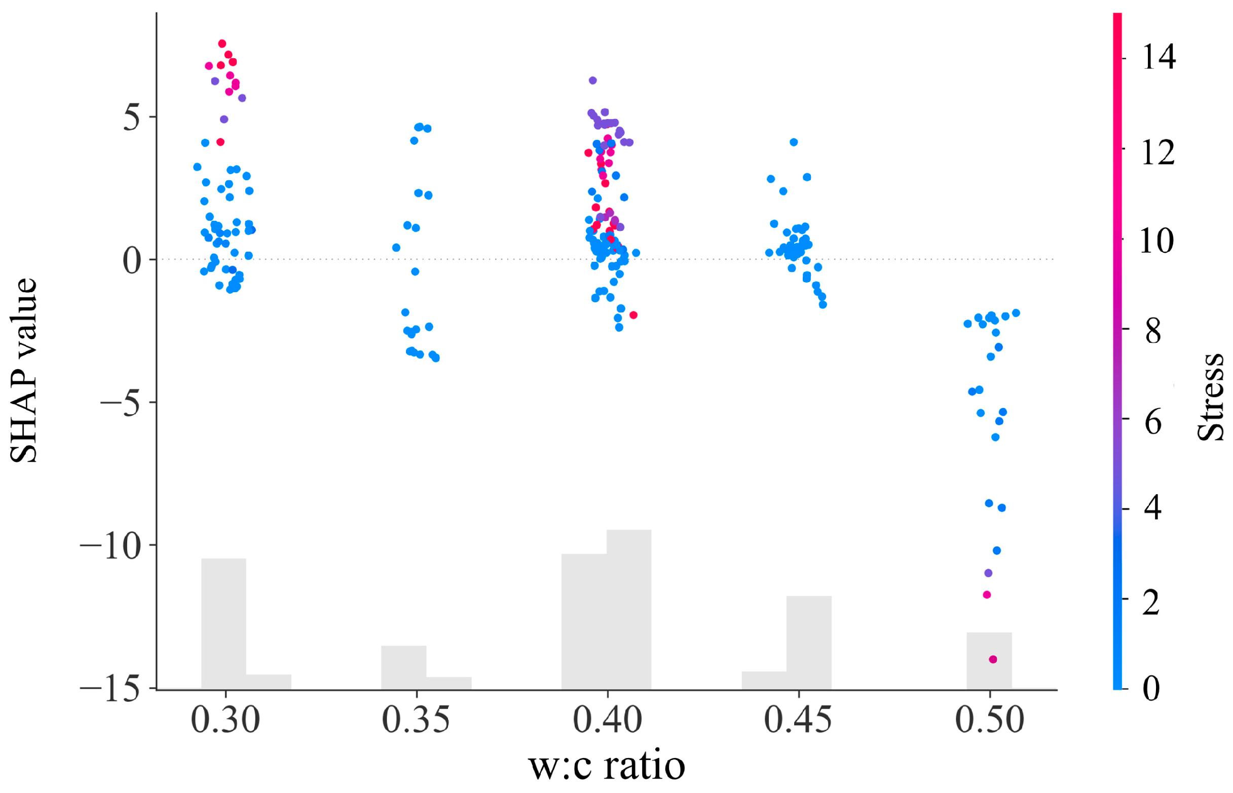
To further elucidate the impact of changes in input variables on the model output, this section will analyze the input variables one by one, as shown in the following figures. Figure 19 is a PDP graph, and Figure 20, Figure 21, Figure 22, Figure 23 and Figure 24 are SHAP scatter plots.
Figure 19 shows the impact of each input variable on the output results of the model. From the graph, it can be seen that increasing stress and E has a positive impact on the predicted shear bond strength, while using the Cable type_standard has a negative impact on the prediction results. The impact of w:c ratio and length on model prediction is not significant.
Figure 20 shows that when stress is less than 5 MPa, the model tends to predict smaller results, whereas when stress exceeds 5 MPa, the model tends to predict larger results, and with the increase in stress, the likelihood of the model producing larger results also increases.
Figure 21 shows that when E is less than 50 GPa, the model tends to predict smaller results, and as E decreases, the predicted results also tend to decrease, whereas when E is greater than 50 GPa, the model tends to predict larger results.
Figure 22 shows that when the cable type is not standard, the model tends to predict larger results, whereas when the cable type is standard, the model tends to predict smaller results. This indicates that the structure improvement can significantly improve the shear bond strength of cable bolts.
Figure 23 shows that when Length is less than 0.25 m, the model tends to predict smaller results, whereas when Length is greater than 0.25 m, the model tends to predict larger results. Meanwhile, when Length is greater than 0.25, the contribution of Length to model prediction does not increase significantly with the increase in Length.
Figure 24 shows that when the water–cement ratio is less than 0.45, it has a slight positive impact on the model’s predictions, and its variation has little effect on the results. However, when the water–cement ratio exceeds 0.45, it has a negative impact on the model’s predictions.

5.2.3. LIME Analysis of Specific Points

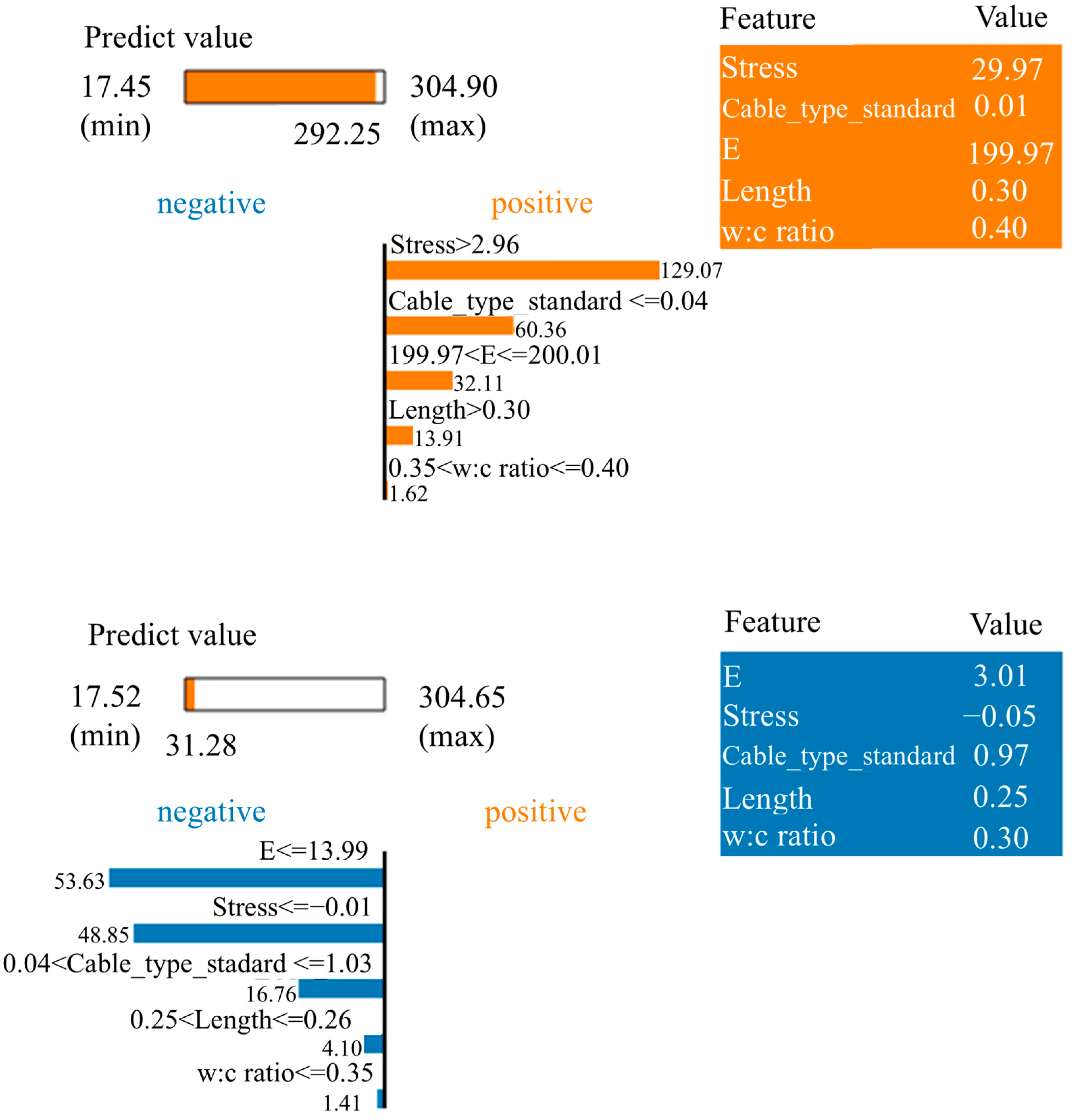
This section will use the LIME method to analyze certain points based on the previous analysis. LIME is very powerful and can analyze the prediction results of the model on specific instances, demonstrating the model’s decision-making process.
For comparison, two points with significant differences were selected. Figure 25 shows that stress and E play a decisive role in model prediction, followed by Cable type_standard, while Length and w:c ratio have little effect. These are consistent with the previous analysis.

6. Conclusions

This study proposed and evaluated three hybrid machine learning models (RF-WOA, RF-TSA, RF-JSO) to predict the shear bond strength of cable bolts based on an augmented dataset. The results demonstrate the effectiveness of integrating metaheuristic optimization algorithms with random forest. Among the models tested, the RF-JSO model achieved the highest prediction accuracy, with R2 values of 0.989 (training set) and 0.981 (testing set), confirming the superiority of the JSO in enhancing model performance.
Model performance was comprehensively evaluated using six statistical metrics (R2, RMSE, MAE, MAPE, VAF, and A-20 index), enabling a robust and balanced assessment. The consistency of high performance across all metrics supports the reliability and stability of the proposed hybrid models. Additionally, SHAP analysis revealed that stress, Cable type_standard, and E are the most influential input variables affecting the model predictions. LIME analysis was used to examine the impact of these critical variables. The identification of key influencing factors such as confining stress, elastic modulus, and cable type provides guidance for optimizing cable bolt design. Specifically, higher confining stress and stiffer host materials (i.e., higher modulus) are associated with greater shear bond strength, suggesting that field conditions should be carefully evaluated to select appropriate bolt types. Furthermore, the finding that non-standard cable types contribute to improved bond strength indicates that structural enhancements in cable design can lead to better performance in challenging ground conditions. These insights support more informed decisions in the selection and application of cable bolts in both laboratory and field scenarios.
Overall, the integration of optimization-based modeling, interpretability analysis, and performance evaluation provides a useful approach for analyzing shear bond strength in the context of cable bolts. This study underscores the impact of combining advanced optimization with explainable AI to create models that are not only accurate but also provide practical, field-relevant guidance, which can assist future researchers in related studies.

Author Contributions

M.X.: Methodology, Formal analysis, Validation, Resources, Visualization, Writing—original draft. Y.Q.: Formal analysis, Writing—review and editing. M.K.: Formal analysis, Investigation, Writing—review and editing, Data curation. M.H.K.: Formal analysis, Writing—review and editing. J.Z.: Conceptualization, Methodology, Validation, Investigation, Visualization, Writing—review and editing, Supervision, Funding acquisition. All authors have read and agreed to the published version of the manuscript.

Funding

This research was partially supported by the National Natural Science Foundation Project of China (52474121 and 42177164).

Data Availability Statement

The raw data supporting the conclusions of this article will be made available by the authors on request.

Conflicts of Interest

The authors declare that they have no known competing financial interests or personal relationships that could have appeared to influence the work reported in this paper.

References

  1. Jahangir, E.; Blanco-Martín, L.; Hadj-Hassen, F.; Tijani, M. Development and application of an interface constitutive model for fully grouted rock-bolts and cable-bolts. J. Rock Mech. Geotech. Eng. 2021, 13, 811–819. [Google Scholar] [CrossRef]
  2. Singh, S.; Srivastava, A.K. Numerical simulation of pull-out test on cable bolts. Mater. Today Proc. 2021, 45, 6332–6340. [Google Scholar] [CrossRef]
  3. Xu, D.-P.; Jiang, Q.; Li, S.-J.; Qiu, S.-L.; Duan, S.-Q.; Huang, S.-L. Safety assessment of cable bolts subjected to tensile loads. Comput. Geotech. 2020, 128, 103832. [Google Scholar] [CrossRef]
  4. Salcher, M.; Bertuzzi, R. Results of pull tests of rock bolts and cable bolts in Sydney sandstone and shale. Tunn. Undergr. Space Technol. 2018, 74, 60–70. [Google Scholar] [CrossRef]
  5. Thenevin, I.; Blanco-Martín, L.; Hadj-Hassen, F.; Schleifer, J.; Lubosik, Z.; Wrana, A. Laboratory pull-out tests on fully grouted rock bolts and cable bolts: Results and lessons learned. J. Rock Mech. Geotech. Eng. 2017, 9, 843–855. [Google Scholar] [CrossRef]
  6. Fu, M.; Huang, S.; Fan, K.; Liu, S.; He, D.; Jia, H. Study on the relationship between the maximum anchoring force and anchoring length of resin-anchored bolts of hard surrounding rocks based on the main slip interface. Constr. Build. Mater. 2023, 409, 134000. [Google Scholar] [CrossRef]
  7. Chen, J.; Saydam, S.; Hagan, P.C. Numerical simulation of the pull-out behaviour of fully grouted cable bolts. Constr. Build. Mater. 2018, 191, 1148–1158. [Google Scholar] [CrossRef]
  8. Chen, J.; Saydam, S.; Hagan, P.C. An analytical model of the load transfer behavior of fully grouted cable bolts. Constr. Build. Mater. 2015, 101, 1006–1015. [Google Scholar] [CrossRef]
  9. Nourizadeh, H.; Mirzaghorbanali, A.; Serati, M.; Mutaz, E.; McDougall, K.; Aziz, N. Failure characterization of fully grouted rock bolts under triaxial testing. J. Rock Mech. Geotech. Eng. 2024, 16, 778–789. [Google Scholar] [CrossRef]
  10. Shahani, N.; Kamran, M.; Zheng, X.; Liu, C. Predictive modeling of drilling rate index using machine learning approaches: LSTM, simple RNN, and RFA. Pet. Sci. Technol. 2022, 40, 534–555. [Google Scholar] [CrossRef]
  11. Kamran, M.; Faizan, M.; Wang, S.; Han, B.; Wang, W.-Y. Generative AI and Prompt Engineering: Transforming Rockburst Prediction in Underground Construction. Buildings 2025, 15, 1281. [Google Scholar] [CrossRef]
  12. Huang, S.; Zhou, J. An enhanced stability evaluation system for entry-type excavations: Utilizing a hybrid bagging-SVM model, GP and kriging techniques. J. Rock Mech. Geotech. Eng. 2025, 17, 2360–2373. [Google Scholar] [CrossRef]
  13. Zhang, Y.-l.; Qiu, Y.-g.; Armaghani, D.J.; Monjezi, M.; Zhou, J. Enhancing rock fragmentation prediction in mining operations: A Hybrid GWO-RF model with SHAP interpretability. J. Cent. South Univ. 2024, 31, 2916–2929. [Google Scholar] [CrossRef]
  14. Ali, F.; Masoud, S.S.; Behnam, F.; Mohamadreza, C. Modeling the load-displacement curve for fully-grouted cable bolts using Artificial Neural Networks. Int. J. Rock Mech. Min. Sci. 2016, 86, 261–268. [Google Scholar] [CrossRef]
  15. Jodeiri Shokri, B.; Mirzaghorbanali, A.; McDougall, K.; Karunasena, W.; Nourizadeh, H.; Entezam, S.; Hosseini, S.; Aziz, N. Data-Driven Optimised XGBoost for Predicting the Performance of Axial Load Bearing Capacity of Fully Cementitious Grouted Rock Bolting Systems. Appl. Sci. 2024, 14, 9925. [Google Scholar] [CrossRef]
  16. Soufi, A.; Zerradi, Y.; Bahi, A.; Souissi, M.; Ouadif, L. Machine Learning Models for Cable Bolt Load-Bearing Capacity in Sublevel Open Stope Mining. Min. Metall. Explor. 2025, 42, 1651–1675. [Google Scholar] [CrossRef]
  17. Bouteldja, M. Design of Cable Bolts Using Numerical Modelling. PhD Dissertation, McGill University, Montreal, QC, Canada, 2000. [Google Scholar]
  18. Breiman, L. Random Forests. Mach. Learn. 2001, 45, 5–32. [Google Scholar] [CrossRef]
  19. He, B.; Armaghani, D.J.; Lai, S.H. Assessment of tunnel blasting-induced overbreak: A novel metaheuristic-based random forest approach. Tunn. Undergr. Space Technol. 2023, 133, 104979. [Google Scholar] [CrossRef]
  20. Zhou, J.; Dai, Y.; Khandelwal, M.; Monjezi, M.; Yu, Z.; Qiu, Y. Performance of Hybrid SCA-RF and HHO-RF Models for Predicting Backbreak in Open-Pit Mine Blasting Operations. Nat. Resour. Res. 2021, 30, 4753–4771. [Google Scholar] [CrossRef]
  21. Kaur, S.; Awasthi, L.K.; Sangal, A.L.; Dhiman, G. Tunicate Swarm Algorithm: A new bio-inspired based metaheuristic paradigm for global optimization. Eng. Appl. Artif. Intell. 2020, 90, 103541. [Google Scholar] [CrossRef]
  22. Mirjalili, S.; Lewis, A. The Whale Optimization Algorithm. Adv. Eng. Softw. 2016, 95, 51–67. [Google Scholar] [CrossRef]
  23. Watkins, W.A.; Schevill, W.E. Aerial Observation of Feeding Behavior in Four Baleen Whales: Eubalaena glacialis, Balaenoptera borealis, Megaptera novaeangliae, and Balaenoptera physalus. J. Mammal. 1979, 60, 155–163. [Google Scholar] [CrossRef]
  24. Chou, J.-S.; Truong, D.-N. A novel metaheuristic optimizer inspired by behavior of jellyfish in ocean. Appl. Math. Comput. 2021, 389, 125535. [Google Scholar] [CrossRef]
  25. Mariottini, G.L.; Pane, L. Mediterranean Jellyfish Venoms: A Review on Scyphomedusae. Mar. Drugs 2010, 8, 1122–1152. [Google Scholar] [CrossRef] [PubMed]
  26. Medawela, S.; Armaghani, D.J.; Indraratna, B.; Kerry Rowe, R.; Thamwattana, N. Development of an advanced machine learning model to predict the pH of groundwater in permeable reactive barriers (PRBs) located in acidic terrain. Comput. Geotech. 2023, 161, 105557. [Google Scholar] [CrossRef]
  27. Mei, X.; Li, C.; Sheng, Q.; Cui, Z.; Zhou, J.; Dias, D. Development of a hybrid artificial intelligence model to predict the uniaxial compressive strength of a new aseismic layer made of rubber-sand concrete. Mech. Adv. Mater. Struct. 2023, 30, 2185–2202. [Google Scholar] [CrossRef]
  28. Gholamy, A.; Kreinovich, V.; Kosheleva, O. Why 70/30 or 80/20 Relation Between Training and Testing Sets: A Pedagogical Explanation. Departmental Technical Reports (CS). 12 March 2018. Available online: https://scholarworks.utep.edu/cs_techrep/1209 (accessed on 12 August 2025).
  29. Pham, B.T.; Jaafari, A.; Prakash, I.; Bui, D.T. A novel hybrid intelligent model of support vector machines and the MultiBoost ensemble for landslide susceptibility modeling. Bull. Eng. Geol. Environ. 2019, 78, 2865–2886. [Google Scholar] [CrossRef]
  30. Hastie, T.; Tibshirani, R.; Friedman, J. Overview of Supervised Learning. In The Elements of Statistical Learning: Data Mining, Inference, and Prediction; Hastie, T., Tibshirani, R., Friedman, J., Eds.; Springer: New York, NY, USA, 2009; pp. 9–41. [Google Scholar]
  31. Taylor, K.E. Summarizing multiple aspects of model performance in a single diagram. J. Geophys. Res. Atmos. 2001, 106, 7183–7192. [Google Scholar] [CrossRef]
  32. Zorlu, K.; Gokceoglu, C.; Ocakoglu, F.; Nefeslioglu, H.A.; Acikalin, S. Prediction of uniaxial compressive strength of sandstones using petrography-based models. Eng. Geol. 2008, 96, 141–158. [Google Scholar] [CrossRef]
  33. Winter, E. Chapter 53 The shapley value. In Handbook of Game Theory with Economic Applications; Elsevier: Amsterdam, The Netherlands, 2002; Volume 3, pp. 2025–2054. [Google Scholar]
  34. Koh, P.W.; Liang, P. Understanding black-box predictions via influence functions. In Proceedings of the 34th International Conference on Machine Learning—Volume 70, Sydney, NSW, Australia, 6–11 August 2017; pp. 1885–1894. [Google Scholar]
  35. Ribeiro, M.T.; Singh, S.; Guestrin, C. “Why Should I Trust You?”: Explaining the Predictions of Any Classifier. In Proceedings of the 22nd ACM SIGKDD International Conference on Knowledge Discovery and Data Mining, San Francisco, CA, USA, 13–17 August 2016; pp. 1135–1144. [Google Scholar]
  36. Ni, Z.; Yang, J.; Fan, Y.; Hang, Z.; Zeng, B.; Feng, C. Multi-factors effects analysis of nonlinear vibration of FG-GNPRC membrane using machine learning. Mech. Based Des. Struct. Mach. 2024, 52, 8988–9014. [Google Scholar] [CrossRef]
  37. Kashem, A.; Karim, R.; Malo, S.; Das, P.; Datta, S.; Alharthai, M. Hybrid data-driven approaches to predicting the compressive strength of ultra-high-performance concrete using SHAP and PDP analyses. Case Stud. Constr. Mater. 2024, 20, e02991. [Google Scholar] [CrossRef]
  38. Zhou, J.; Xu, M.; Li, C. Prediction of dam failure peak outflow using a novel explainable random forest based on metaheuristic algorithms. J. Hydrol. 2025, 662, 133767. [Google Scholar] [CrossRef]
  39. Nikmah, T.L.; Syafei, R.M.; Muzayanah, R.; Salsabila, A.; Nurdin, A.A. Prediction Of Used Car Prices Using K-Nearest Neighbour, Random Forest and Adaptive Boosting Algorithm. Indones. Community Optim. Comput. Appl. 2023, 1, 17–22. [Google Scholar]
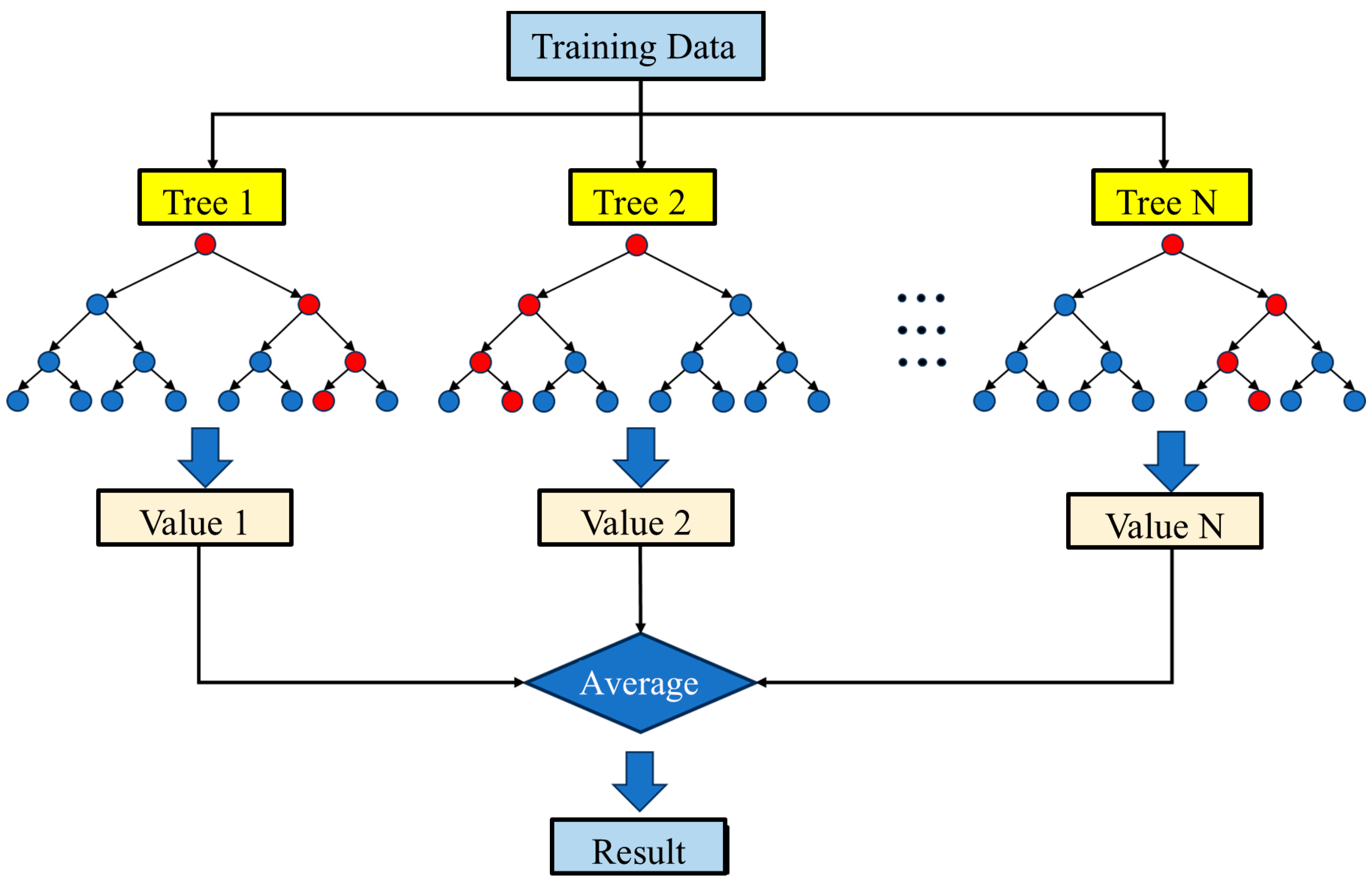
Figure 1. The structure of random forest.
Machines 13 00758 g001
Figure 2. The search process of TSA.
Machines 13 00758 g002
Figure 3. The bubble-net predation method of humpback whales.
Machines 13 00758 g003
Figure 4. JSO flowchart.
Machines 13 00758 g004
Figure 5. Contribution analysis chart of input variables.
Machines 13 00758 g005
Figure 6. Matrix plot of variables.
Machines 13 00758 g006
Figure 7. Data distribution before data augmentation.
Machines 13 00758 g007
Figure 8. Data distribution after data augmentation.
Machines 13 00758 g008
Figure 9. Flowchart of model construction. (a) model training phase; (b) model testing and selection phase.
Machines 13 00758 g009
Figure 10. Iteration process of the three hybrid models.
Machines 13 00758 g010
Figure 11. Taylor diagram to evaluate the performance of the model: (a) training stage, (b) testing stage.
Machines 13 00758 g011
Figure 12. Bar charts comparing the performance of the hybrid models and the standard RF model on the test set.
Machines 13 00758 g012
Figure 13. Comparison of predicted and actual values of RF-WOA model.
Machines 13 00758 g013
Figure 14. Comparison of predicted and actual values of RF-TSA model.
Machines 13 00758 g014
Figure 15. Comparison of predicted and actual values of RF-JSO model.
Machines 13 00758 g015
Figure 16. Sensitivity analysis of the n_estimators and max_depth hyperparameters.
Machines 13 00758 g016
Figure 17. Shapley beeswarm diagram analysis of RF-JSO model.
Machines 13 00758 g017
Figure 18. Comparison of the contributions of each input variable.
Machines 13 00758 g018
Figure 19. PDP analysis results.
Machines 13 00758 g019
Figure 20. Impact analysis of stress.
Machines 13 00758 g020
Figure 21. Impact analysis of E.
Machines 13 00758 g021
Figure 22. Impact analysis of Cable type_standard.
Machines 13 00758 g022
Figure 23. Impact analysis of Length.
Machines 13 00758 g023
Figure 24. Impact analysis of w:c ratio.
Machines 13 00758 g024
Figure 25. LIME analysis results of two specific points.
Machines 13 00758 g025
Table 1. Variance Inflation Factor (VIF) for input features.
FeatureVIF Value
E1.255409
Length1.045857
w:c ratio1.085248
Stress1.385977
Cable_type_standard1.235832
Table 2. Obtained hyperparameters from different hybrid models.
Hyper-ParametersRangeRFRF-WOARF-JSORF-TSA
n_estimators[50–400]1009521373
max_depth[1–20]Default1099
min_samples_leaf[1–50]Default433
min_samples_split[2–50]Default222
max_features.[1–50]Default666
Table 3. Comparison of performance scores between the initial RF model and three hybrid models.
StageModelR2ScoreRMSEScoreMAEScoreMAPEScoreVAFScoreA-20ScoreFinal Score
Training setRF0.99645.36742.72144.7499.57240.972424
RF-WOA0.99138.23234.12838.5399.11330.922318
RF-TSA0.98928.46214.50419.7298.92110.91729
RF-JSO0.98928.35124.43629.7298.94920.917212
Testing setRF0.968114.2417.216117.5196.83610.89949
RF-WOA0.98311.41526.55528.9498.05320.899417
RF-TSA0.981411.21636.55239.2398.11530.888218
RF-JSO0.981411.06346.45749298.16840.891321
Table 4. Comparison performance of the best model in this study with two benchmark models.
StageModelR2RMSEMAEMAPEVAFA-20
Training setRF-JSO0.9898.3514.4369.798.90.917
XGBoost0.978012.0838.1251898.90.814
LGBM0.9819.2356.1321198.10.845
Test setRF-JSO0.98111.0636.457998.10.891
XGBoost0.97113.6179.11814.197.20.798
LGBM0.967614.5939.39513.496.70.817
Disclaimer/Publisher’s Note: The statements, opinions and data contained in all publications are solely those of the individual author(s) and contributor(s) and not of MDPI and/or the editor(s). MDPI and/or the editor(s) disclaim responsibility for any injury to people or property resulting from any ideas, methods, instructions or products referred to in the content.