An Improved Black-Winged Kite Algorithm for High-Accuracy Parameter Identification of a Photovoltaic Double Diode Model

Abstract

This study proposes an improved Black-Winged Kite Algorithm (SRQ-BKA) for accurate parameter identification of the photovoltaic (PV) double diode model (DDM). The proposed method integrates three key mechanisms: specular reflection learning (SRL) to improve initial population diversity, preventing premature convergence and enabling a more comprehensive exploration of the solution space for optimal parameters; soft rime search (SRS) to balance global exploration and local exploitation, ensuring efficient identification by dynamically adjusting the search focus; and quadratic interpolation (QI) to accelerate convergence by fine-tuning the search toward optimal parameters, enhancing accuracy and speeding up the identification process. The root mean square error (RMSE) is employed as the objective function to minimize the error between the measured and predicted I-V characteristics of the PV module. Experimental results demonstrate that the SRQ-BKA outperforms other algorithms, achieving a minimum RMSE of 0.00262 A for the DDM and exhibiting strong stability, as evidenced by an average RMSE of 0.00278 A across 1000 runs. The method also demonstrates excellent parameter identification accuracy for both the single diode model (SDM) and triple diode model (TDM), further validating its robustness and practical applicability.

1. Introduction

In the context of the global energy transition and sustainable development, photovoltaic (PV) energy has emerged as one of the most promising renewable energy sources because of its cleanliness, renewability, and widespread availability [1]. However, the output characteristics of PV cells exhibit strong nonlinear interactions among irradiance, ambient temperature, and intrinsic parameters, making precise modeling and parameter identification critical for enhancing system efficiency. Constructing high-precision PV cell models enables the effective optimization of maximum power point tracking algorithms [2], the evaluation of battery degradation, and the facilitation of fault diagnosis through theoretical analysis. Therefore, research on PV cell modeling holds substantial engineering significance for advancing the deployment and optimization of PV technology in industrial applications.

The mainstream equivalent circuit models for PV cells currently include the single diode model (SDM), double diode model (DDM), and triple diode model (TDM) [3]. The SDM is a simplified version of the DDM, designed to reduce complexity by representing the PV cell’s behavior with a single diode branch. Although the SDM is widely adopted because of its simplicity and reduced number of parameters, this simplification compromises the accurate modeling of critical mechanisms, including carrier recombination and thermal effects. As a result, the SDM tends to produce significant errors, especially under low-irradiance or partial-shading conditions. In contrast, the DDM introduces a second diode branch to more accurately model carrier recombination, thereby significantly enhancing the accuracy of modeled I-V characteristics, particularly under challenging environmental conditions [4]. However, the increased model complexity poses challenges for parameter identification because solving the nonlinear equations is difficult and computationally inefficient [5]. Although the TDM further refines the decomposition of current components, it is hindered by its excessive number of parameters and high hardware implementation costs, which limit its widespread adoption [6]. Furthermore, PV cell models can be classified as implicit or explicit according to their mathematical expressions: explicit models employ the Lambert W function or approximate analytical methods to obtain rapid solutions but sacrifice some physical fidelity [7]; implicit models preserve the complete physical mechanisms, accurately describe the I-V characteristics of PV cells, and are more intuitive and easier to derive. The implicit DDM provides distinct advantages in applications that demand high modeling accuracy, particularly in scenarios where physical fidelity is critical. With its seven unknown parameters, the DDM exhibits strong nonlinearity and multivariable coupling, resulting in challenges such as a high-dimensional search space and susceptibility to local optima, thereby necessitating the development of efficient and reliable parameter-identification algorithms [8].

Traditional parameter-identification methods primarily rely on analytical approaches, such as the Lambert W function, and on numerical iterative methods, such as the Newton–Raphson method; however, these methods are highly sensitive to initial values and often struggle with complex nonlinear problems [7]. In recent years, metaheuristic algorithms (MAs) have gained prominence in parameter identification because of their strong global search capability and gradient-free characteristics. Inspired by natural phenomena, physical laws, and social behaviors, these algorithms simulate dynamic processes to search for global optima [9]. Based on the origin of their core concepts, MAs are categorized into four groups: evolutionary algorithms (EAs), physics-based algorithms (PAs), human-inspired algorithms (HAs), and swarm-intelligence algorithms (SAs).

Evolutionary algorithms (EAs) emulate biological evolution, emphasizing natural selection and genetic operators. Representative algorithms include the genetic algorithm (GA) [10], differential evolution (DE) [11], marine predators algorithm (MPA) [12], etc. Physics-based algorithms (PAs) are inspired by the energy minimization principles or thermodynamic laws governing physical systems. These include the equilibrium optimizer (EO) [13], atom search algorithm (ASO) [14], snow ablation optimizer (SAO) [15], rime optimization algorithm (RIME) [16], etc. Human behavior-based algorithms (HAs) are inspired by human interactions and social processes. Notable examples include teaching-learning-based optimization (TLBO) [17], social network optimization (SNO) [18], and the cooperation search algorithm (CSA) [19], etc. Swarm-intelligence algorithms (SAs) achieve optimization by simulating the cooperative behaviors of biological groups, including particle swarm optimization (PSO) [20], the whale optimization algorithm (WOA) [21], gray wolf optimizer (GWO) [22], artificial gorilla troops optimizer (GTO), Black-Winged Kite Algorithm (BKA) [23], etc. Notably, Wang et al. proposed the BKA in 2024 as a novel swarm-intelligence method. By simulating the kite’s precise local search during the predation phase and global exploration during migration, it overcomes the single-behavior limitation of traditional swarm algorithms, demonstrating excellent global-optimization capability and adaptability. However, its core limitations become apparent when applied to the parameter identification of high-dimensional nonlinear systems. The algorithm relies heavily on random migration and simple attack behaviors, which leads to population homogenization and a higher risk of becoming trapped in local optima. Its attack strategy employs fixed perturbation patterns without intelligent guidance, resulting in low local-search accuracy. Moreover, it lacks mathematical acceleration strategies and relies solely on random search. As a result, the algorithm often requires numerous iterations to effectively solve high-dimensional problems.

Recent studies have demonstrated that hybrid optimization algorithms leverage complementary strategies to dynamically balance exploration and exploitation throughout the search process. For instance, Chen et al. employed a maximum-power matching strategy combined with an improved FDA (IFDA) to identify model parameters, which significantly enhanced both convergence speed and accuracy [24]. Jiang et al. proposed a composite method (CGH-GTO) that integrates the improved gray wolf optimizer (IGWO), the hummingbird algorithm (HBA), and the artificial gorilla troops optimizer (GTO), thereby improving both the accuracy and speed of model parameter identification [25]. Chen et al. combined the teaching-learning-based optimization (TLBO) and the artificial bee colony (ABC) algorithm to propose a hybrid method, TLABC, for solar PV parameter estimation [26]. Long et al. proposed a hybrid algorithm (GWOCS) based on the gray wolf optimizer (GWO) and cuckoo search (CS), which achieved an effective balance between exploration and exploitation and demonstrated good robustness in PV model parameter extraction [27].

Building upon these insights, recent studies have further advanced the design of hybrid metaheuristics by incorporating domain-specific knowledge and multi-strategy fusion. Alsaggaf et al. [28] introduced a chemistry-inspired material generation algorithm (MGA) that mimics ionic and covalent bonding to enhance parameter estimation for PV models. Hakmi et al. [29] developed a modified rime-ice growth optimizer (MRIME) integrated with a polynomial differential learning operator (PDLO), achieving superior RMSE minimization on the RTC France and STM6-40/36 modules. Additionally, Qian et al. [30] proposed a multi-strategy fused Kepler optimization algorithm (MKOA) leveraging good point set initialization, dynamic opposition-based learning, and normal cloud model perturbation, demonstrating robust performance in both benchmark tests and real-world engineering applications. These developments underscore the effectiveness of tailored hybrid strategies in addressing the nonlinear and multimodal characteristics of PV parameter identification.

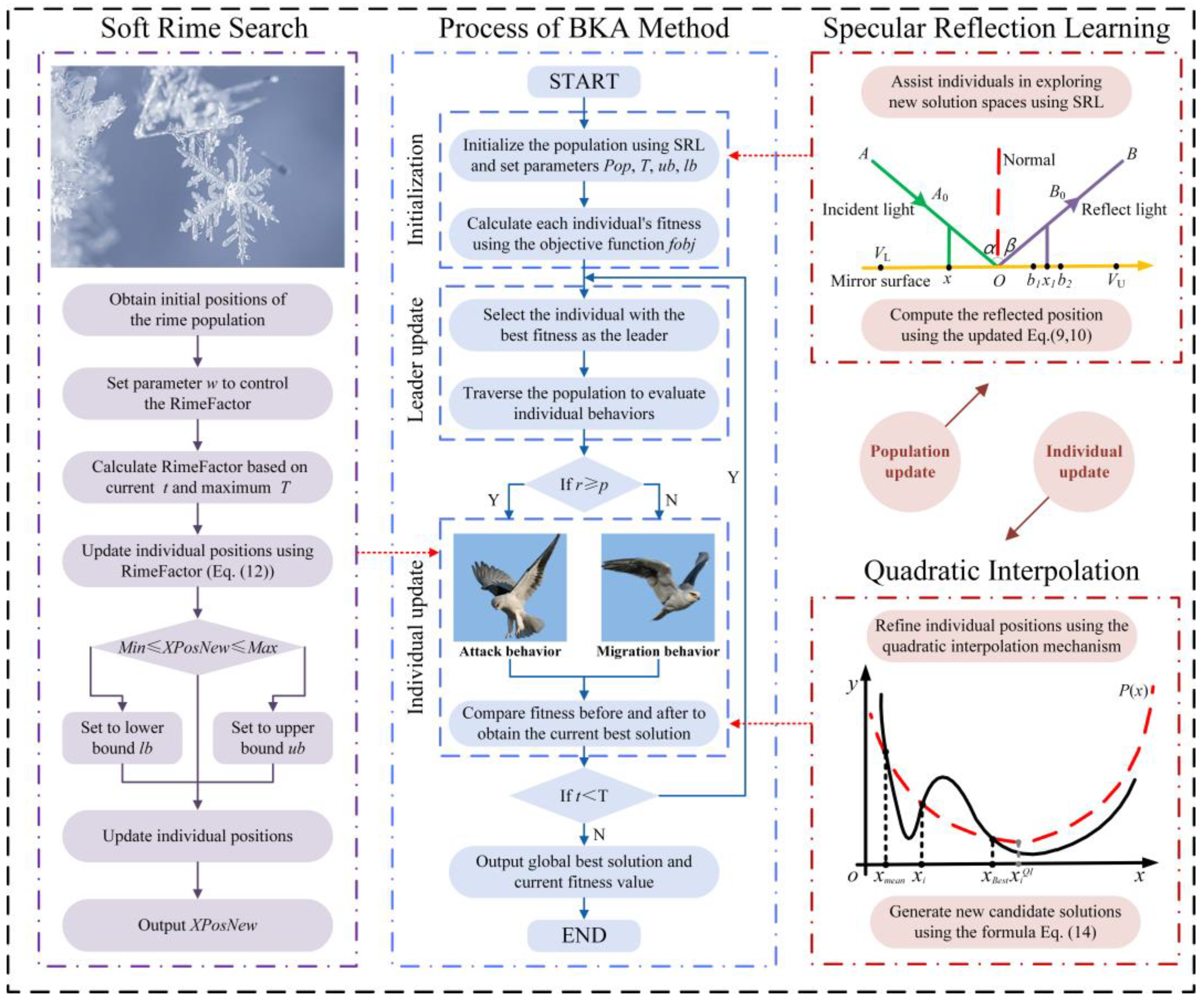
Inspired by these findings, this work aims to enhance the performance of the BKA by embedding targeted hybrid mechanisms tailored to the characteristics of PV model parameter identification. To the best of our knowledge, this study is the first to integrate SRL, SRS, and QI into the BKA framework, yielding a novel metaheuristic termed the SRQ-BKA. This algorithm is designed to overcome the limitations of the BKA, including limited population diversity, inadequate local search capability, and slow convergence in multimodal landscapes. Specifically, SRL is employed to enhance population diversity and prevent premature convergence. Subsequently, SRS balances global exploration and local exploitation, whereas QI accelerates convergence and refines solutions near the optima. This integrated design enables the SRQ-BKA to achieve more accurate, robust, and stable parameter identification across diverse environmental conditions. Finally, the effectiveness and engineering applicability of the SRQ-BKA are validated through comprehensive benchmark tests and real-world PV experiments. Figure 1 illustrates the structural composition and operational flow of the proposed SRQ-BKA. In summary, the key contributions of this paper are as follows:

• SRL is introduced into the BKA for the first time to generate high-quality initial solutions via specular reflection, thereby improving population diversity and providing a stronger foundation for accurate and reliable parameter identification.
• A hybrid optimization strategy that combines SRS and QI is proposed to enhance search efficiency. SRS enhances exploration during the early stages and gradually promotes exploitation as iterations progress, whereas QI refines the local search by accelerating convergence toward the optimal parameters.
• A progressive experimental design verifies the SRQ-BKA from theory to application. Benchmark tests confirm its rapid convergence and strong global search capability. Experiments on PV models demonstrate high accuracy, robustness, and practical applicability.

Section 2 introduces the fundamental concepts and operational stages of the BKA. Section 3 provides details of the proposed SRQ-BKA, emphasizing the integration of SRL, SRS, and QI to enhance optimization performance. Section 4 presents experimental validation using benchmark functions and PV model parameter identification. Section 5 concludes the study.

2. Black-Winged Kite Algorithm

Based on the hunting strategy and migratory characteristics of the black-winged kite, Wang et al. proposed a novel swarm-intelligence algorithm, the BKA [23]. The algorithm consists of three distinct stages: the initialization phase, the attacking phase, and the migratory phase.

2.1. Initialization Stage

The BKA employs a random initialization method to generate the initial population within the upper and lower bounds of the search space. This process can be mathematically expressed as follows:

$$P_i=B{K}_{lb}+rand\left(B{K}_{ub}-B{K}_{lb}\right)$$

(1)

where P_i represents the i-th individual, i ∈ 1,2,…, N. BK_lb and BK_ub are the lower and upper bounds of the j-th dimension of the black-winged kite, and rand is a uniformly distributed random number in the interval [0, 1].

2.2. Attacking Stage

In this stage, the BKA simulates the predatory behavior of the black-winged kite: individuals adjust the angles of their wings and tails according to the wind speed to observe and attack prey during flight. The mathematical model of the black-winged kite’s attack behavior is described by Equations (2) and (3).

$$y_{t+1}^{i,j}=\left\{\begin{array}{l}{y}_t^{i,j}+n\left(1+\sin (r)\right)y_t^{i,j},p<r\hfill \\ y_t^{i,j}+n (2r-1)y_t^{i,j},else\hfill \end{array}\right.$$

(2)

$$n=0.05\exp \left(-2{(t/T)}^2\right)$$

(3)

where $y_t^{i,j}$ and $y_{t+1}^{i,j}$ denote the positions of the i-th black-winged kite in the j-th dimension at the t-th and (t + 1)-th iteration steps, respectively; r is a random number between 0 and 1; p is a constant equal to 0.9; n is a nonlinear factor; t is the number of iterations completed so far; and T is the total number of iterations.

2.3. Migratory Stage

The migration phase simulates the migratory behavior of birds driven by environmental factors. The BKA assumes that if an individual’s current fitness exceeds that of a randomly selected peer from the population, it leads the population to migrate toward the destination; otherwise, it lacks leadership and joins the migrating group. The migratory behavior of the black-winged kite is described by mathematical models, as shown in Equations (4) and (5).

$$y_{t+1}^{i,j}=\left\{\begin{array}{l}{y}_t^{i,j}+C(0,1)\left(y_t^{i,j}-L_t^j\right),F_i<F_{ri}\hfill \\ y_t^{i,j}+C(0,1)\left(L_t^j-m{y}_t^{i,j}\right),\mathrm{else}\hfill \end{array}\right.$$

(4)

$$m=2\sin (r+\pi /2)$$

(5)

where $L_t^j$ represents the current best-known position of the BKA in the j-th dimension at iteration t. F_i denotes the fitness of the i-th black-winged kite at iteration t. F_ri is the fitness value of a randomly selected individual from the population at iteration t. C(0, 1) represents the Cauchy mutation operator with a location parameter of 0 and a scale parameter of 1.

3. SRQ-BKA for Model Parameter Identification

The BKA often falls into local optima during the search process, especially for complex optimization problems, indicating that both its efficiency and accuracy can be improved. Therefore, this chapter proposes an improved algorithm, named the SRQ-BKA, aimed at enhancing the accuracy of model parameter identification. As shown in Figure 2, the algorithm integrates three mechanisms—SRL, SRS, and QI—that collectively enhance its search ability and convergence precision. SRL improves the initial solution quality of the original BKA and enhances the robustness of its global search. SRS refines the random attack behavior of the original BKA through a staged perturbation strategy, thereby improving the controllability of the search direction. QI uses mathematical modeling to approximate extreme points directly, which significantly reduces the number of local exploitation iterations and accelerates convergence.

3.1. Construction of Fitness Function

The DDM is a critical physical model for characterizing the output behavior of solar cells. Its equivalent circuit, shown in Figure 3, comprises a photocurrent source, two parallel diodes, a series resistor, and a parallel resistor.

By introducing a second diode, this model more accurately captures carrier recombination mechanisms within the semiconductor [31], especially recombination effects in the space-charge region, allowing it to maintain high accuracy even under non-standard test conditions [32]. The mathematical expression of the DDM for the PV module is given below [33].

$$I=I_{ph}-I_{01}\left[\exp \left({\displaystyle \frac{V+NI{R}_s}{N{A}_1{V}_{th}}}\right)-1\right]-I_{02}\left[\exp \left({\displaystyle \frac{V+NI{R}_s}{N{A}_2{V}_{th}}}\right)-1\right]-{\displaystyle \frac{V+NI{R}_s}{N{R}_{sh}}}$$

(6)

where I and V are the current and voltage. I₀₁ and I₀₂ are the saturation currents of the two diodes, respectively. R_s and R_sh indicate the equivalent series resistance and equivalent parallel resistance, respectively. A₁ and A₂ are ideal factors. V_th is the thermal voltage and the equation is V_th = kT/q. k denotes the Boltzmann constant, which takes the value of 1.381 × 10⁻²³ J/K. T is the temperature of the PV cell. q represents the electron charge, with a value of 1.602 × 10⁻¹⁹ C. N is the number of cells in a PV module.

For the parameter identification problem of the DDM, the fitness function is typically constructed based on the error between measured I-V data and model predictions [34]. The standard formulation of the fitness function is given by

$$\mathrm{RMSE}=\sqrt{{\displaystyle \frac{1}{n}}\sum _{i=1}^n{\left(I_{\mathrm{measure},i}-I_{\mathrm{theory},i}\right)}^2}$$

(7)

where I_measure,i refers to the experimentally measured current, I_theory,i denotes the model-predicted current, and n indicates the number of points sampled on the I-V curve.

3.2. Model Parameter Initialization Method Based on SRL

The precision and convergence rate of MAs strongly depend on the quality of the initial population. Considering the different value ranges of the seven model parameters [35], a normalized transformation is applied to scale each parameter to its corresponding bounds, which addresses this issue and improves the efficiency of parameter identification [24].

$$\left[\begin{array}{c}{I}_{ph}\\ I_{01}\\ I_{01}\\ A_1\\ A_2\\ R_s\\ R_{sh}\end{array}\right]=\left[\begin{array}{c}6x_1\\ {10}^{\left(3x_2\right)}\\ {10}^{\left(3x_3\right)}\\ x_4\\ x_5\\ \left(0.5{\lambda }_1{x}_6+\mu \right)N\\ \left(0.5{\lambda }_2{x}_7+\mu \right)N\end{array}\right]$$

(8)

where λ₁ = 5/N, λ₂ = 1000/N, and μ = 5 × 10⁻⁴/N. N is the number of cells connected in series.

To further enhance the quality of the initial population, this study employs SRL, a novel learning strategy inspired by the physical phenomenon of specular reflection [36]. This strategy is closely related to opposition-based learning (OBL) and can be regarded as a generalized form of OBL. By generating mirror solutions within the solution space, SRL improves both search efficiency and population diversity, thereby strengthening the algorithm’s capability to locate the global optimum.

In specular reflection, the incident and reflected rays are symmetric with respect to the normal line, as illustrated in Figure 2. Inspired by this phenomenon, SRL generates a corresponding mirror solution for each candidate in the solution space. This symmetry forms the foundation of SRL, enabling the algorithm to simultaneously consider a solution and its mirror counterpart during the search, thereby increasing the likelihood of finding superior solutions.

In SRL, the mirror solution is not strictly opposite but instead lies within a localized neighborhood around the opposite solution. The size of this neighborhood is controlled by a flexibility coefficient λ, enabling SRL to generate a richer set of candidate solutions in the search space, thereby enhancing both local search capability and global optimization potential.

$$\overline{x}=(0.5\lambda +0.5)\times (V_L+V_U)-\lambda x$$

(9)

where V_L and V_U represent the lower and upper bounds of the variable, respectively, and λ is the elasticity coefficient controlling the neighborhood size. Specifically, when λ = 1, the mirror solution degenerates to the opposite solution; when λ ≠ 1, the mirror solution lies within a neighborhood near the opposite solution. This design enables SRL to generate a broader variety of candidate solutions, effectively enhancing the algorithm’s capabilities for both local exploitation and global exploration. The calculation formula for λ is as follows:

$$\lambda =\left\{\begin{array}{ll}1+\varphi R_0,\hfill & \mathrm{if} {\kappa }_1>{\kappa }_2\hfill \\ 1-\varphi R_0,\hfill & \mathrm{if} {\kappa }_1\le {\kappa }_2\hfill \end{array}\right.$$

(10)

where κ₁ and κ₂ are two random numbers in the range [0, 1]; R₀ is the neighborhood radius, and ϕ is the elasticity coefficient, also ranging between 0 and 1. The value of λ, which controls the location of the mirror solution, is dynamically adjusted by comparing κ₁ and κ₂. This dynamic adjustment mechanism allows SRL to perform more flexible and adaptive searches within the solution space.

Once the mirror solution is generated, boundary control is applied to ensure its feasibility within the predefined search domain:

$${\overline{x}}_i=\left\{\begin{array}{ll}{l}_i,\hfill & \mathrm{if} {\overline{x}}_i<l_i\hfill \\ u_i,\hfill & \mathrm{if} {\overline{x}}_i>u_i\hfill \\ {\overline{x}}_i,\hfill & \mathrm{otherwise} \hfill \end{array}\right.$$

(11)

where l_i and u_i represent the lower and upper bounds of the i-th variable, respectively. If the mirror solution x_i is less than l_i, it is set to l_i; if x_i exceeds u_i, it is set to u_i; otherwise, it remains unchanged. This boundary control strategy ensures that the resulting solutions remain feasible and eliminates invalid candidates from the search process.

Furthermore, the proposed approach merges the original and mirror solutions and selects the top 50% of high-quality individuals based on their fitness values. This mechanism effectively eliminates low-quality solutions, improves the average fitness of the initial population compared to random initialization, and significantly increases the density of solutions in high-quality regions. Consequently, it provides more favorable initial conditions for the subsequent evolutionary process.

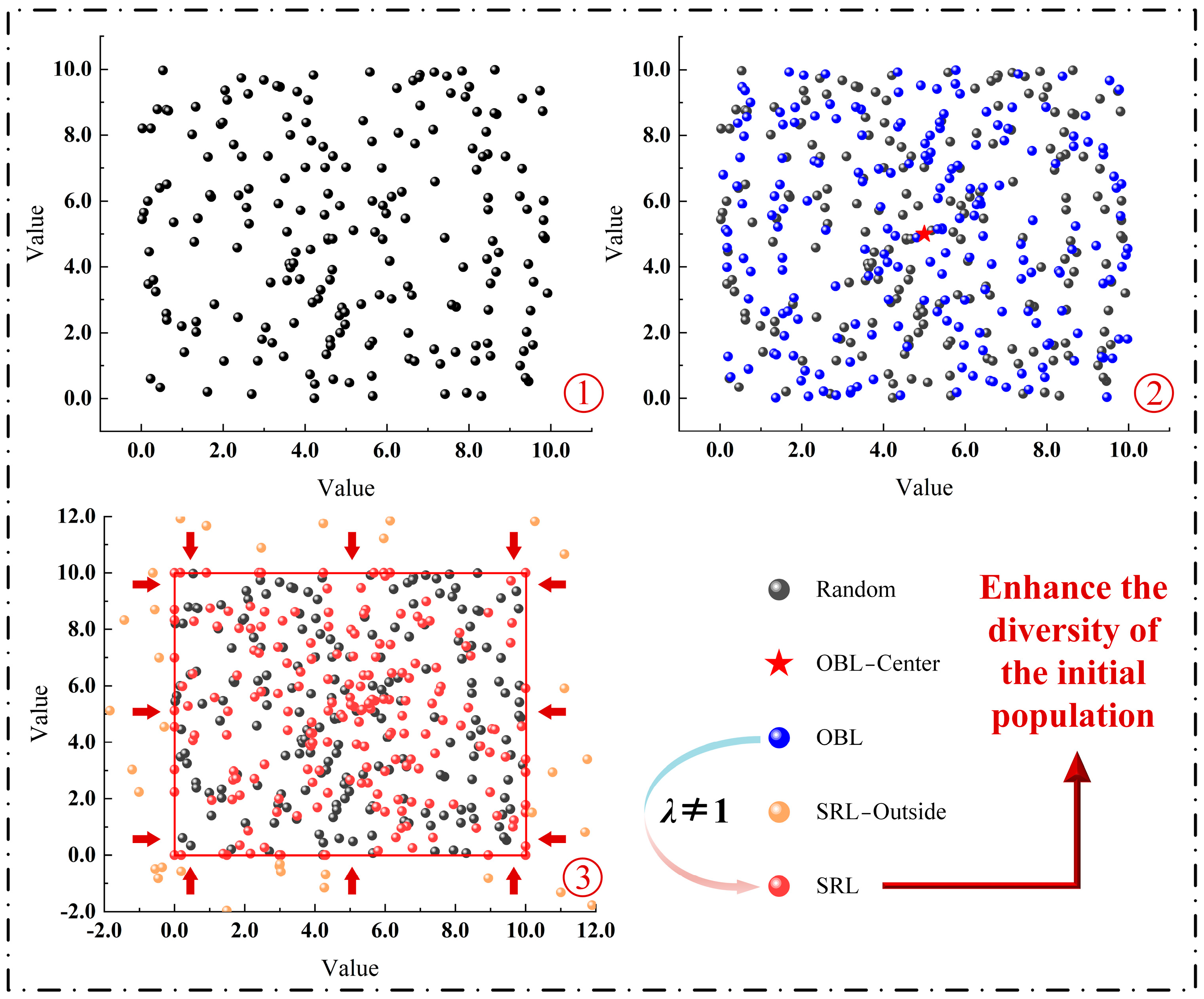
Compared with random initialization, SRL enhances both population diversity and quality through dynamic mirror-based mapping and selective refinement, producing a more diverse and higher-quality initial population for subsequent optimization. To validate the effectiveness of SRL, Figure 4 compares the initial population distributions of random initialization, OBL, and SRL within the original boundary range of [0, 10]. The randomly initialized population exhibits irregular clustering, leaving large gaps in some regions of the search space. Although OBL yields a symmetric distribution about the central axis, it remains strictly confined within the original range, making it inflexible and less effective in exploring boundary regions. Conversely, SRL generates a solution set that extends beyond the original boundaries through the dynamic elasticity factor, thereby enhancing diversity and reducing the risk of early stagnation in local optima. During mirror-solution generation, SRL allows temporary excursions beyond the boundary, which are then truncated to retain feasible components. Thus, SRL effectively enhances the initial exploration capability of MAs, providing a robust and efficient foundation for global search.

3.3. Hybrid Optimization with SRS and QI for Efficient Search

Building on the initial population enhancement achieved through SRL, SRS is subsequently introduced to further optimize the search process. SRS is derived from RIME, which was proposed by Su et al. [16] based on the natural rime crystallization process. It mimics the growth of soft rime and thereby achieves a balance between exploration and exploitation. As shown in Figure 2, SRS follows a distinctive staged process that dynamically switches between broad exploration and fine-grained exploitation, thereby achieving both efficiency and precision.

The growth of soft rime exhibits pronounced stochasticity, allowing frost particles to spread randomly over the surface, while directional growth is relatively slow and gradually stabilizes under environmental constraints.

Following the dynamic behavior of rime particles, their position updates can be expressed mathematically as follows:

$$\left\{\begin{array}{l}{R}_{ij}^{new }=R_{best,j }+r_1\cdot \cos \theta \cdot \beta \cdot \left(\psi \cdot \left(U{b}_{ij}-L{b}_{ij}\right)+L{b}_{ij}\right)\hfill \\ r_2<E\hfill \end{array}\right.$$

(12)

where $R_{ij}^{new}$ denotes the updated position of the particle, while R_best,j represents the j-th particle of the best crystal in the rime particle population R. r₁ is a uniformly distributed random value in the range (−1, 1), used to modulate the direction of particle motion, which is further influenced by the directional cosine cosθ during the optimization process. β represents an environmental factor, and ψ ∈ [0, 1] denotes the particle adhesion coefficient, which controls the inter-particle spacing. Ub_ij and Lb_ij denote the upper and lower bounds of the particle’s motion space, respectively. r₂ ∈ (0, 1), together with the adhesion coefficient E, determines whether the particle condenses, that is, whether its position is updated. The following condition must be satisfied to ensure convergence.

$$\left\{\begin{array}{c}\theta =\pi \cdot {\displaystyle \frac{t}{10\cdot T}}\\ \beta =1-\left[{\displaystyle \frac{w\cdot t}{T}}\right]/w\\ E=\sqrt{(t/T)}\end{array}\right.$$

(13)

where t represents the current iteration number, and T denotes the maximum number of iterations. β is a step function, and w is a control parameter that determines the number of segments in the function, with w set to 5. E denotes the adhesion coefficient, which progressively increases over iterations and regulates the probability of particle condensation during the search process.

SRS is incorporated into the attack behavior of the BKA through a cosine-driven perturbation factor. This mechanism enhances global exploration with larger perturbations during early iterations and gradually shifts to refined local search as the perturbations stabilize. This dynamic adjustment improves the balance between exploration and exploitation, helping prevent premature convergence and optimizing the subsequent search process.

QI is then applied to accelerate convergence by fitting a quadratic curve through the current solution and its neighboring elite solutions. QI is a technique for estimating the value of a function based on a set of known data points [37]. In MAs, the algorithm’s convergence rate heavily depends on the search step size. If the step size is too small, the algorithm may stagnate at local minima, whereas an excessively large step size may cause it to miss the global optimum. By fitting a local quadratic approximation of the objective function, QI estimates the optimal step size and effectively guides the algorithm toward the global optimum with faster convergence.

The core idea of QI in this study is to fit a parabolic curve to the objective function using three points: the current individual, the population mean, and the leader. The minimum of the fitted parabola is then taken as an approximation of the objective function’s minimum. This mathematically guided search enhances both the stability of convergence and the precision of the optimization process.

After updating the leader position, the algorithm computes the population mean position and average fitness, identifies the global best position, and selects the i-th individual for interpolation. A QI curve is then constructed using these three reference points. The fitted curve is expressed as P(x) = a₀x² + a₁x + a₂. The vertex of the fitted parabola, x_i^QI serves as the estimated optimum obtained through the QI method. In most cases, the QI strategy produces candidate solutions with higher fitness than the original ones. The mathematical formulation of QI is given as follows.

$$\left\{\begin{array}{l}N=\left(x_i^2-x_{\mathrm{mean} }^2\right)\times F_{\mathrm{best} }+\left(x_{\mathrm{mean} }^2-x_{\mathrm{best} }^2\right)\times F_i+\left(x_{\mathrm{best} }^2-x_i^2\right)\times F_{\mathrm{mean} }\hfill \\ D=\left(x_i-x_{\mathrm{mean} }\right)\times F_{\mathrm{best} }+\left(x_{\mathrm{mean} }-x_{\mathrm{best} }\right)\times F_i+\left(x_{\mathrm{best} }-x_i\right)\times F_{\mathrm{mean} }\hfill \\ x_i^{QI}={\displaystyle \frac{N}{2D}}\hfill \end{array}\right.$$

(14)

where x_i, x_mean, and x_best denote the positions of the i-th individual, the centroid of the population, and the current best solution in the swarm, respectively. F_i, F_mean, and F_best correspond to the fitness values of the i-th individual, the average fitness of the population, and the best fitness achieved so far. Finally, a greedy selection strategy is employed to retain the better solution between x_i and the interpolated candidate $x_i^{QI}$.

$$x_i^{\prime }=\left\{\begin{array}{l}{x}_i^{QI}, \mathrm{if} F\left(x_i\right)>F\left(x_i^{QI}\right)\hfill \\ x_i, \mathrm{otherwise} \hfill \end{array}\right.$$

(15)

where $x_i^{\prime }$ represents the retained individual with higher fitness.

3.4. SRQ-BKA

This section elaborates on the enhancement strategies applied to the BKA within the SRQ-BKA framework. A visual representation of the improved methodology is shown in Figure 2.

In the proposed SRQ-BKA, the random initialization in the original BKA is replaced with the SRL strategy described earlier, and the algorithm proceeds with the attack phase. This stage is inspired by avian hunting behavior, where individuals adjust their wing and tail angles according to wind velocity to observe and attack targets during flight. SRS is embedded into the attack behavior of the BKA through a cosine-driven perturbation factor, which enables adaptive modulation of the step size during iterations. The refined mathematical formulation of the attack mechanism in the SRQ-BKA, incorporating SRS, is given in Equations (16) and (17).

$$y_{t+1}^{i,j}=\left\{\begin{array}{l}{y}_t^{i,j}+n\cdot \left(1+\sin (r)\cdot y_t^{i,j}\right),p<r\hfill \\ y_t^{i,j}+RimeFactor\cdot [\psi \cdot (B{K}_{ub}^j-B{K}_{lb}^j)+B{K}_{lb}],\mathrm{else}\hfill \end{array}\right.$$

(16)

$$\left\{\begin{array}{l}n=0.05\exp \left(-2{(t/T)}^2\right)\hfill \\ RimeFactor=2(r-0.5)\cdot \cos \left({\displaystyle \frac{\pi \cdot t}{10\cdot T}}\right)·(1-{\displaystyle \frac{round(t\cdot w/T)}{w}})\hfill \end{array}\right.$$

(17)

where $y_t^{i,j}$ and $y_{t+1}^{i,j}$ represent the position of the i-th black-winged kite in the j-th dimension at iteration t and t + 1, respectively. r is a stochastic value randomly drawn from the interval [0, 1]. p denotes a fixed parameter with a value of 0.9. n is a nonlinear adjustment factor. ${BK}_{lb}^j$ and ${BK}_{ub}^j$ refer to the lower and upper boundaries of the search range in the j-th dimension, respectively. ψ ∈ [0, 1] is a random parameter used to regulate the update dynamics. t is the current number of completed iterations. T is the maximum number of iterations. The control parameter w is set to 5. RimeFactor is the frost simulation factor.

During early iterations, RimeFactor exhibits large oscillations, generating significant perturbations that enhance global exploration capability. In later iterations, the perturbations gradually stabilize, enabling more refined local search. Integrating dynamic perturbations into the attack behavior allows the algorithm to gradually shift from global exploration to localized exploitation, effectively mitigating premature convergence and instability issues observed in the original BKA.

The final phase involves migration behavior. This stage emulates the environmentally driven migratory behavior observed in birds. In the BKA, it is assumed that if an individual exhibits better fitness than a randomly selected peer from the population, it will guide the migration toward the destination; otherwise, it lacks leadership and joins the migrating group.

In complex parameter identification tasks, the original BKA update strategy may produce imprecise position updates, especially in multimodal problems where it fails to effectively locate the global optimum. To address this issue, after completing the attack and migration behaviors, the QI method is introduced to refine the position update process. By applying QI using the current individual, the global leader, and the population mean, the strategy balances global exploration and local refinement, enhancing search accuracy and ensuring convergence to superior solutions. Building on these enhancements,

Table 1. Structural and performance differences between the BKA and SRQ-BKA.

Aspect	BKA	SRQ-BKA	Improvement
Initialization	Random	SRL	Better diversity
Attacking phase	Sinusoidal update	Sinusoidal + SRS	Balanced exploration–exploitation
Migration phase	Cauchy peer comparison	Same as original	Retained for global exploration
Local refinement	Not included	QI	Improved convergence and accuracy
Overall structure	Basic movement strategy	SRL + SRS + QI	More adaptive and stable optimization
Application	Moderate accuracy	High accuracy, robust under varying conditions	Better practical use

provides a comparative summary of the original BKA and the proposed SRQ-BKA, emphasizing the architectural improvements and their influence on convergence speed and solution accuracy.

To better illustrate the integration of SRL, SRS, and QI modules, the complete pseudocode of the SRQ-BKA is presented in

Table 2. Pseudocode of the SRQ-BKA.

Algorithm: SRQ-BKA

Input:

N: population size. T: maximum iterations.

D: solution dimension. [lb, ub]: search bounds.

f(x): objective function.

Output:

Best_Pos: best solution. Best_Fit: best fitness value.

1:    Initialize population X within [lb, ub]

2:    Evaluate fitness of X and set Best_Pos, Best_Fit

3:    for t = 1 to T do

4:            Sort population and update Best_Pos

5:            // SRL: Specular Reflection Learning

6:            Generate mirrored candidates from elite individuals

7:            Replace individuals if mirrored candidates perform better

8:            for each X_i in population do

9:              // Attacking phase

10:            Update X_i via sinusoidal or Soft Rime Search (SRS)

11:            // Migration phase

12:            Adjust X_i using Cauchy-based peer comparison

13:            // QI: Quadratic Interpolation refinement

14:            Generate new candidate from X_i, mean(X), and Best_Pos

15:            Replace X_i if the new candidate improves fitness

16:        end for

17:        Record Best_Fit

18: end for

19: Return Best_Pos, Best_Fit

. Although these enhancements improve search performance, they introduce minimal additional computational overhead, preserving overall algorithmic efficiency. The overall time complexity of the algorithm is O(T⋅N⋅D), where T denotes the number of iterations, N is the population size, and D refers to the dimensionality of the optimization problem, representing the number of parameters to be identified. This complexity is consistent with that of the original BKA, as the additional strategies introduce only lightweight operations in each generation. Therefore, the algorithm significantly improves performance without a notable increase in computational burden.

4. Experiments and Verification

The experimental I-V characteristic measurement system is schematically illustrated in Figure 5. The system consists of four primary functional units:

• Test PV module (TSM-240). This multicrystalline silicon module has the following key specifications under standard test conditions (STC): short-circuit current I_sc = 8.62 A, open-circuit voltage V_oc = 37.3 V, and maximum power P_max = 240 W. Additional parameters and detailed specifications are listed in

  Table 3. Specification of TSM-240 under STC.

  Parameter	Symbol	Value
  Maximum power	Pmax,stc	240 W
  Voltage at maximum power point	Vmax,stc	29.7 V
  Current at maximum power point	Imax,stc	8.1 A
  Short-circuit current	Isc,stc	8.62 A
  Open-circuit voltage	Voc,stc	37.3 V
  Temperature coefficient of Isc	αstc	0.047%/°C.
  Temperature coefficient of Voc	βstc	−0.32%/°C.
  Number of cells in series	Np	60

  .
• I-V acquisition module. A microcontroller governs the relay-based switching to dynamically acquire the I-V characteristics of the tested PV module.
• Environmental monitoring unit. It is equipped with a pyranometer and temperature sensors to continuously record the irradiance (W/m²) and the surface temperature (°C).
• Data processing system. The collected I-V and environmental data are transmitted to an industrial computer through an RS-485 serial interface, where dedicated software displays the real-time I-V curves and extracts key performance parameters.

The experiments were conducted on the rooftop of the laboratory building at Hohai University in Changzhou, China, which has a typical subtropical monsoon climate. Three representative environmental scenarios were selected to capture the PV module performance under varying operating conditions: Condition 1: irradiance of 379 W/m² and temperature of 27.9 °C; Condition 2: irradiance of 590 W/m² and temperature of 36.5 °C; Condition 3: irradiance of 900 W/m² and temperature of 47.8 °C. These datasets comprehensively reflect the actual output characteristics of the PV module under diverse environmental conditions.

The monitoring software allows real-time tracking of I-V curve variations and provides essential experimental data for analyzing the influence of environmental conditions on PV module behavior. Analysis shows that increasing temperature reduces the open-circuit voltage, while higher irradiance leads to a significant rise in short-circuit current. These findings provide valuable guidance for optimizing PV system design and performance evaluation.

4.1. Evaluation Methods

The model parameter identification method was evaluated using five performance indicators: RMSE, mean absolute error (MAE), mean absolute percentage error (MAPE), the coefficient of determination (R²), and computation time (C_time). The RMSE is calculated using Equation (7), while the formulas for MAE, MAPE, and R² are given in Equations (18)–(20) [38]. All experiments were conducted on MATLAB R2023b using a computer equipped with an Intel Core i9-13900HX (2.20 GHz), 32 GB RAM, and Windows 11. C_time was directly recorded using the experimental platform.

$$\mathrm{MAE}={\displaystyle \frac{1}{n}}\sum _{i=1}^n\left|I_{\mathrm{measure},i}-I_{\mathrm{theory},i}\right|$$

(18)

$$\mathrm{MAPE}={\displaystyle \frac{100\%}{n}}\sum _{i=1}^n\left|{\displaystyle \frac{I_{\mathrm{measure},i}-I_{\mathrm{theory},i}}{I_{\mathrm{measure},i}}}\right|$$

(19)

$${\mathrm{R}}^2=1-{\displaystyle \frac{{\displaystyle \sum _{i=1}^n}{\left(I_{\mathrm{measure},i}-I_{\mathrm{theory},i}\right)}^2}{{\displaystyle \sum _{i=1}^n}{\left(I_{\mathrm{mean}}-I_{\mathrm{theory},i}\right)}^2}}$$

(20)

where I_mean represents the average value of the measured current.

Notably, both the original BKA and the proposed SRQ-BKA used the same number of function evaluations, as they adopted identical population sizes and iteration counts. This ensures a fair comparison because any observed performance improvement arises solely from the SRQ-BKA’s algorithmic enhancements rather than increased computational effort.

4.2. Experiment 1: Comparison of Optimization Results for Benchmark Test Functions

To verify the effectiveness of the BKA improvements, three benchmark test functions were first optimized, and the results were compared with those obtained using the BKA, GTO, GWO, SAO, RIME, DE, GA, and TLBO. These methods represent the four categories of metaheuristic algorithms (MAs) summarized in the Introduction. The objective functions used to assess optimization performance are shown in

Table 4. Benchmark test function details.

Code	Function	Domain
F5	$y={\displaystyle \sum _{i=1}^{n-1}}[100{(x_{i+1}-x_i^2)}^2+{(x_i-1)}^2]$	[−30, 30]
F7	$y={\displaystyle \sum _{i=1}^n}i{x}_i^4+random[0,1)$	[−1.28, 1.28]
F10	$y=-20\exp (-0.2\sqrt{{\displaystyle \frac{1}{n}}{\displaystyle \sum _{i=1}^n}{x}_i^2})-\exp ({\displaystyle \frac{1}{n}}{\displaystyle \sum _{i=1}^n}\cos (2\pi x_i))+20+e$	[−32, 32]

. The selected benchmark functions cover a wide range of optimization challenges, including both smooth and non-smooth as well as unimodal and multimodal problems. This selection aimed to evaluate the algorithm’s performance in diverse scenarios, focusing on robustness, global search capability, and the ability to escape local optima. Employing diverse benchmark functions allows a comprehensive evaluation of the algorithm’s performance across various optimization challenges.

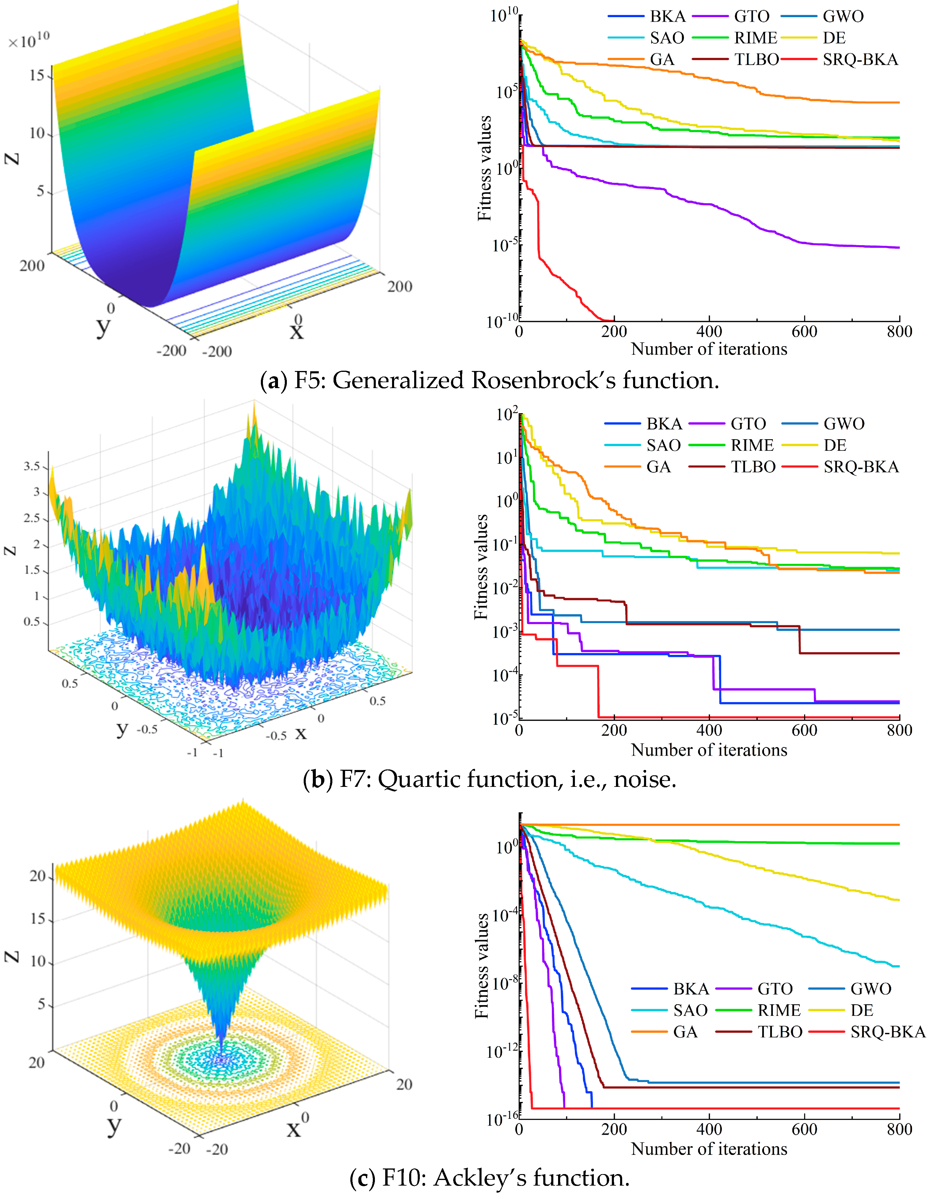
The F5 function, known as the Rosenbrock function, features a narrow, curved parabolic valley. It is commonly used to assess an algorithm’s ability to converge to the global optimum in complex local landscapes, particularly evaluating its capability to escape local minima. The F7 function incorporates quartic terms and random noise, which evaluate an algorithm’s robustness and noise resistance, making it suitable for validating convergence accuracy and result stability. The F10 function, derived from the Ackley function, is a typical multimodal function containing many local minima and is highly sensitive to initial solutions. It is particularly suitable for evaluating the global search capability of optimization algorithms and their effectiveness in escaping local optima.

The minimum value of each benchmark function was obtained with different MAs, and the iteration speed and search capability of each algorithm were subsequently compared. Figure 6 illustrates the iteration processes of the algorithms for the benchmark problems. In Figure 6, the 3D plot on the left shows the objective function landscape, and the convergence curve on the right depicts the relationship between fitness values and iteration counts for each optimization algorithm. Clearly, the SRQ-BKA (red curve) converged faster to a lower objective function value than the other algorithms, demonstrating superior optimization performance and rapid convergence. This result highlights the efficiency and accuracy of the SRQ-BKA in attaining the optimal solution.

In PV diode model parameter identification, the model functions typically exhibit nonlinearity, multi-parameter coupling, and complex solution spaces, requiring optimization algorithms with strong global search capability, robustness, and rapid convergence. The excellent performance of the SRQ-BKA on F5 and F7 directly corresponds to typical PV modeling problems, indicating its superior suitability for high-precision fitting. Additionally, its strong global search capability on the F10 function helps prevent the algorithm from becoming trapped in local optima during parameter identification, thereby enhancing model generalization and predictive accuracy. Therefore, the SRQ-BKA not only performs well in standard tests but also demonstrates strong potential for practical applications in PV model parameter identification.

4.3. Experiment 2: Parameter Identification of DDM Based on Measured Data

Experimental comparisons of nine methods for model parameter identification were conducted using three sets of measured I-V curves. The identification results were presented in five forms: the fitness iteration process, I-V curves, P-V curves, radar charts, and box plots. These results demonstrate the parameter identification performance of the nine methods and validate the superiority of the SRQ-BKA.

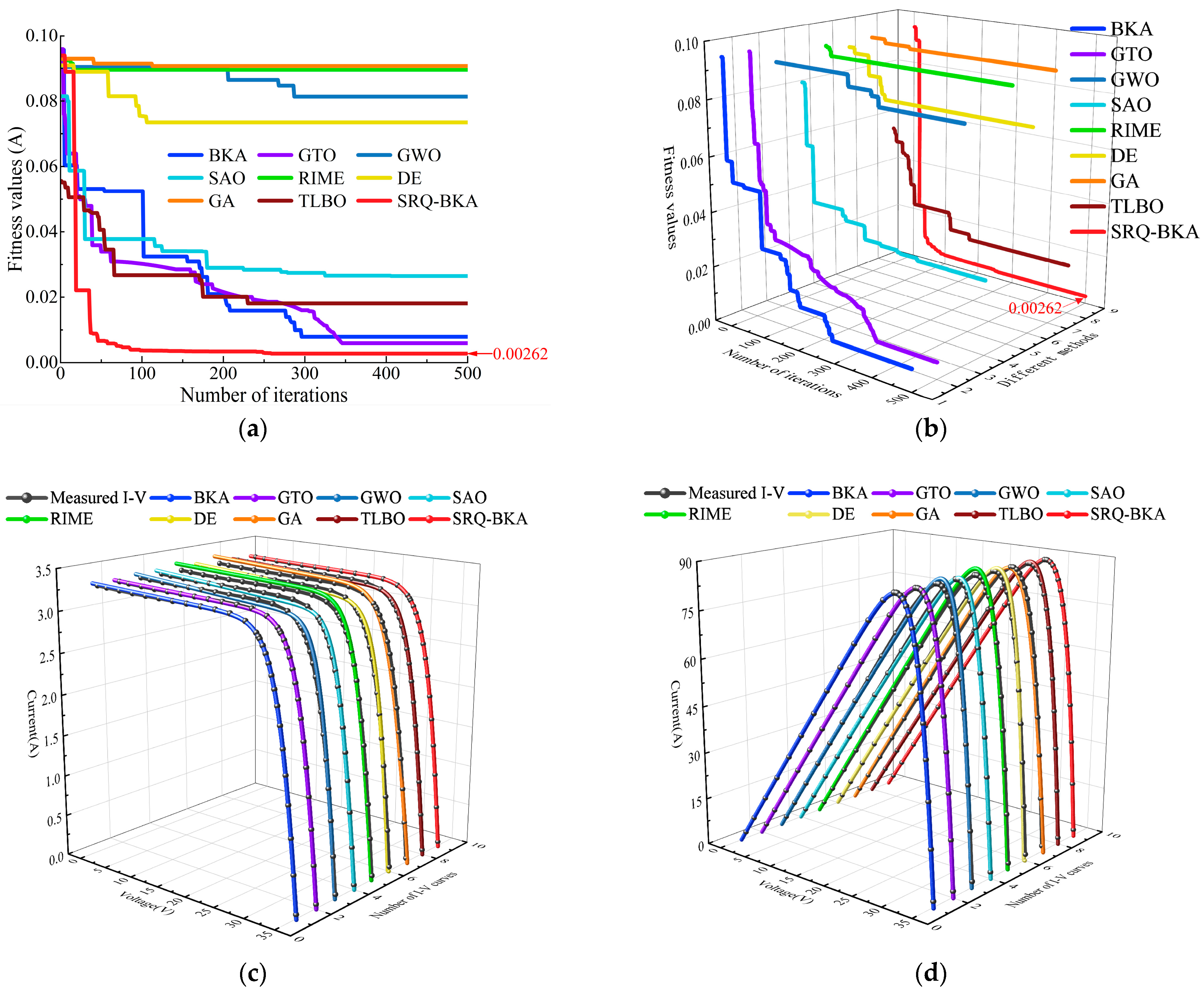
Figure 7, Figure 8 and Figure 9a,b illustrate the iteration curves of the nine methods during model parameter identification. The red curve represents the SRQ-BKA, which exhibits rapid convergence and high accuracy. The final fitness values of the SRQ-BKA for the three sets of measured I-V curves were 0.00262 A, 0.00671 A, and 0.00823 A, respectively. The iteration curves of the GA, RIME, and GWO exhibit only minor variations, confirming their weaker optimal-search capability for the seven parameters. DE, SAO, and TLBO show more pronounced fluctuations in their iteration curves; however, these approaches lack sufficient sensitivity and converge relatively slowly. The final fitness values of these three methods generally exceeded 0.015 A. Notably, the BKA and GTO performed well, with final fitness values falling below 0.01 A. However, compared with the SRQ-BKA, these methods exhibited slower convergence and lower computational accuracy.

As shown in Figure 7, Figure 8 and Figure 9, subplots (c) and (d), respectively, display the nine theoretical I-V and P-V curves generated from the three sets of measured I-V curves. The dark gray solid lines in the figures represent the measured I-V and P-V data, and the alignment between the theoretical and measured curves visually reflects the accuracy of the different parameter identification methods. Analysis indicates that the theoretical curves obtained by the GA, RIME, and GWO deviate markedly from the measured data, indicating lower parameter-identification accuracy for these methods. Although the theoretical curves generated by DE, SAO, and TLBO follow the general trend of the measured data, noticeable deviations remain, suggesting that the identification accuracy of these methods requires further improvement. In contrast, the BKA and GTO performed better, with theoretical curves showing only slight deviations, demonstrating higher parameter-identification accuracy. Notably, the SRQ-BKA exhibited the best fitting performance, with its theoretical curves almost completely overlapping the measured data and showing no discernible visual difference. This demonstrates that the SRQ-BKA has excellent parameter-identification capability and can accurately represent the PV module’s performance.

To further quantify the fitting accuracy,

Table 5. Measured and estimated I-V data with error metrics under Condition 1 (379 W/m², 27.9 °C) using the proposed method.

Voltage (V)	Measured Current (A)	Estimated Current (A)	Absolute Error (A)	Relative Error (%)
0.340	3.294	3.294	0.000	0.008
2.753	3.285	3.286	0.001	0.034
5.165	3.278	3.279	0.001	0.016
7.578	3.272	3.272	0.000	0.007
9.990	3.268	3.268	0.000	0.012
12.403	3.266	3.267	0.001	0.023
14.815	3.264	3.264	0.000	0.010
17.228	3.262	3.264	0.002	0.063
19.640	3.259	3.261	0.002	0.075
22.053	3.253	3.252	0.001	0.019
24.465	3.238	3.240	0.002	0.047
26.878	3.185	3.185	0.000	0.005
28.600	3.082	3.082	0.000	0.012
28.950	3.047	3.049	0.002	0.073
29.140	3.025	3.023	0.002	0.074
29.630	2.957	2.955	0.002	0.073
30.087	2.879	2.876	0.003	0.087
30.543	2.781	2.783	0.002	0.063
31.000	2.660	2.661	0.001	0.055
31.457	2.518	2.520	0.002	0.077
31.913	2.345	2.348	0.003	0.107
32.370	2.139	2.141	0.002	0.073
32.827	1.891	1.891	0.000	0.011
33.283	1.607	1.608	0.001	0.092
33.740	1.284	1.282	0.002	0.156
34.197	0.917	0.918	0.001	0.080
34.653	0.506	0.504	0.002	0.369
35.110	0.060	0.062	0.002	3.883

,

Table 6. Measured and estimated I-V data with error metrics under Condition 2 (590 W/m², 36.5 °C) using the proposed method.

Voltage (V)	Measured Current (A)	Estimated Current (A)	Absolute Error (A)	Relative Error (%)
0.540	5.152	5.152	0.000	0.006
2.777	5.139	5.138	0.001	0.022
5.103	5.129	5.131	0.002	0.039
7.430	5.123	5.126	0.003	0.051
9.757	5.120	5.120	0.000	0.001
12.083	5.117	5.113	0.004	0.080
14.410	5.114	5.112	0.002	0.032
16.737	5.110	5.112	0.002	0.036
19.063	5.103	5.103	0.000	0.006
21.390	5.093	5.093	0.000	0.003
23.717	5.072	5.074	0.002	0.033
26.043	4.980	4.978	0.002	0.035
27.750	4.793	4.794	0.001	0.028
27.920	4.765	4.766	0.001	0.011
27.950	4.760	4.764	0.004	0.089
28.230	4.707	4.707	0.000	0.010
28.787	4.581	4.581	0.000	0.005
29.345	4.421	4.419	0.002	0.055
29.902	4.219	4.219	0.000	0.002
30.460	3.983	3.981	0.002	0.039
31.017	3.689	3.686	0.003	0.083
31.575	3.334	3.337	0.003	0.078
32.132	2.915	2.915	0.000	0.003
32.690	2.458	2.460	0.002	0.076
33.247	1.949	1.951	0.002	0.087
33.805	1.365	1.362	0.003	0.221
34.362	0.703	0.699	0.004	0.556
34.920	0.046	0.041	0.005	9.881

and

Table 7. Measured and estimated I-V data with error metrics under Condition 3 (900 W/m², 47.8 °C) using the proposed method.

Voltage (V)	Measured Current (A)	Estimated Current (A)	Absolute Error (A)	Relative Error (%)
0.900	7.883	7.886	0.003	0.032
2.952	7.875	7.871	0.004	0.052
5.133	7.869	7.870	0.001	0.017
7.315	7.864	7.867	0.003	0.037
9.497	7.859	7.859	0.000	0.003
11.678	7.854	7.855	0.001	0.017
13.860	7.848	7.846	0.002	0.032
16.042	7.839	7.837	0.002	0.025
18.223	7.827	7.824	0.003	0.042
20.405	7.807	7.806	0.001	0.009
22.587	7.743	7.742	0.001	0.018
24.768	7.552	7.552	0.000	0.005
25.970	7.315	7.317	0.002	0.027
26.180	7.260	7.257	0.003	0.039
26.400	7.198	7.199	0.001	0.019
27.000	7.001	7.001	0.000	0.001
27.613	6.755	6.755	0.000	0.006
28.227	6.459	6.461	0.002	0.026
28.840	6.109	6.110	0.001	0.010
29.453	5.699	5.699	0.000	0.006
30.067	5.223	5.224	0.001	0.024
30.680	4.666	4.667	0.001	0.013
31.293	4.046	4.043	0.003	0.067
31.907	3.365	3.362	0.003	0.097
32.520	2.625	2.622	0.003	0.111
33.133	1.819	1.817	0.002	0.094
33.747	0.951	0.944	0.007	0.754
34.360	0.053	0.056	0.003	5.978

present detailed comparisons of the measured and estimated I-V data under three representative environmental conditions. Each sampling point includes the voltage, the measured current, the estimated current from the proposed method, as well as the absolute and relative errors. The results consistently exhibit small point-wise errors under all operating conditions. Notably, most relative errors remained below 0.1%, even under high irradiance and temperature, confirming the method’s excellent fitting accuracy and generalization capability, consistent with the previous analysis.

Figure 10 visually compares the performance of nine methods in terms of the RMSE, MAE, MAPE, R², and C_time using radar charts. Figure 10a specifically compares the RMSE performance of the nine methods. In this radar chart, each algorithm’s performance is shown for the three experimental groups. The SRQ-BKA clearly stands out, with RMSE values consistently closest to the chart center, indicating its superior ability to minimize prediction errors across all three groups. This demonstrates that the SRQ-BKA achieves high overall accuracy and effective error control in parameter-identification tasks.

In contrast, the RMSE values of the GA, RIME, and GWO lie near the outer edge of the radar chart, indicating poor prediction accuracy. These methods produce larger errors, making them less reliable for parameter-identification tasks. This result highlights their limited ability to escape local optima and handle complex data structures effectively.

DE, SAO, and TLBO performed better than the GA, RIME, and GWO, with RMSE values closer to the chart center, although still higher than those of the SRQ-BKA. These algorithms demonstrated moderate accuracy but fell short of achieving the precision level of the SRQ-BKA. The BKA and GTO performed similarly to the SRQ-BKA, with RMSE values fairly close but slightly higher, indicating somewhat lower efficiency in error reduction. Notably, although this RMSE difference appears small, it can significantly affect I-V curve fitting. Accurate I-V modeling is crucial for power estimation, improving MPPT efficiency, and enabling effective fault detection. Even slight current-estimation errors can propagate under dynamic irradiance or partial shading, leading to reduced energy yield over time. Therefore, minimizing the RMSE is essential for reliable PV system modeling.

Figure 10a clearly demonstrates the SRQ-BKA’s outstanding RMSE performance, highlighting its effectiveness in error minimization and clear advantage over other methods. Figure 10b,c further emphasize this trend by comparing algorithm performance based on the MAE and MAPE. In both subfigures, the SRQ-BKA remains closest to the center, demonstrating its ability to minimize both absolute and percentage errors across all three groups. In contrast, the GA, RIME, and GWO lie near the outer edges of the radar chart, reflecting poor performance with higher MAE and MAPE values. DE, SAO, and TLBO show moderate performance, lying between the center and the outermost edge, but still falling behind the SRQ-BKA. The BKA and GTO perform similarly to the SRQ-BKA but exhibit slightly higher MAE and MAPE values, indicating somewhat weaker performance. Overall, the analysis of Figure 10a–c consistently demonstrates that the SRQ-BKA excels in error minimization and achieves high predictive accuracy across these key metrics.

R² indicates the consistency between the theoretical curves obtained by the nine methods and the measured curves. In Figure 10d, the R² values of the GA, RIME, and GWO are noticeably lower than those of the other methods. This further confirms the weakness of these three methods in seven-parameter identification. Additionally, the R² distribution of DE and SAO shows significant deviations between the computed I-V curves and the measured I-V curves. These results indicate that the seven-parameter optimal search performance of DE and SAO is also poor. The R² values of the other four methods overlap considerably, indicating that R² alone cannot clearly distinguish the strengths and weaknesses of the nine methods. Therefore, R² is suitable as an evaluation metric but not as a fitness function. Regarding the C_time radar chart, the GA and TLBO required more computation time than the other methods. The C_time value of the SRQ-BKA was located closer to the chart center. This indicates that the SRQ-BKA required comparatively less computation time.

Table 8. Evaluation metrics of 9 methods under conditions (379 W/m², 27.9 °C).

Method	RMSE (A)	MAE (A)	MAPE (%)	R2	Ctime (s)
BKA	0.00793	0.00704	0.85622	0.99989	22.12215
GTO	0.00596	0.00514	0.62538	0.99996	23.65441
GWO	0.08145	0.07193	8.23591	0.99271	22.35456
SAO	0.02653	0.02026	2.33716	0.99917	21.87894
RIME	0.08961	0.07929	9.73165	0.99165	28.54568
DE	0.07355	0.06466	6.16545	0.99322	27.57654
GA	0.09079	0.08038	9.85653	0.99124	54.72315
TLBO	0.01813	0.01357	1.07163	0.99970	31.54447
SRQ-BKA	0.00262	0.00193	0.13107	0.99999	23.33585

,

Table 9. Evaluation metrics of 9 methods under conditions (590 W/m², 36.5 °C).

Method	RMSE (A)	MAE (A)	MAPE (%)	R2	Ctime (s)
BKA	0.00959	0.00757	0.73643	0.99995	19.48948
GTO	0.00876	0.00694	0.69541	0.99996	21.75889
GWO	0.08854	0.07756	15.63727	0.99624	21.08694
SAO	0.03359	0.03081	2.56456	0.99958	17.74258
RIME	0.09402	0.08024	12.13256	0.99492	24.98591
DE	0.06413	0.05613	6.65565	0.99793	23.84567
GA	0.09113	0.07931	13.59581	0.99587	37.46544
TLBO	0.02722	0.02463	1.86554	0.99967	28.15786
SRQ-BKA	0.00671	0.00512	0.52945	0.99998	22.15682

and

Table 10. Evaluation metrics of 9 methods under conditions (900 W/m², 47.8 °C).

Method	RMSE (A)	MAE (A)	MAPE (%)	R2	Ctime (s)
BKA	0.00963	0.00778	0.38146	0.99998	20.67865
GTO	0.00856	0.00690	0.32955	0.99999	21.08977
GWO	0.09631	0.08504	8.57161	0.99862	18.46703
SAO	0.02742	0.02484	3.20456	0.99983	12.54764
RIME	0.09513	0.08405	8.54563	0.99877	23.54232
DE	0.05355	0.04644	7.88791	0.99959	22.45343
GA	0.09725	0.08507	15.4655	0.99856	34.44596
TLBO	0.03504	0.03181	4.69872	0.99978	25.63715
SRQ-BKA	0.00823	0.00673	0.32714	0.99999	22.75781

list the five evaluation metrics for the nine methods. For the SRQ-BKA, the RMSE, MAE, MAPE, R², and C_time for the first group (379 W/m², 27.9 °C) were 0.00262, 0.00193, 0.13107, 0.99999, and 23.34 s, respectively. For the second group (590 W/m², 36.5 °C), the evaluation metrics were 0.00671, 0.00512, 0.52945, 0.99998, and 22.16 s, respectively. For the third group (900 W/m², 47.8 °C), the evaluation metrics were 0.00823, 0.00673, 0.32714, 0.99999, and 22.76 s, respectively. The SRQ-BKA achieved the lowest RMSE, MAE, and MAPE among the nine methods. The SRQ-BKA yielded the highest R² among the nine methods, indicating that its theoretical I-V curve was nearly identical to the measured curve. The C_time of the SRQ-BKA was approximately 23 s, placing it in the upper tier among the nine methods. The conclusions drawn from these tables are consistent with those from Figure 7, Figure 8, Figure 9 and Figure 10, confirming the superior accuracy of the SRQ-BKA.

Table 11. Identified DDM parameters under different environmental conditions by the SRQ-BKA.

Parameter	Condition 1 (379 W/m2, 27.9 °C)	Condition 2 (590 W/m2, 36.5 °C)	Condition 3 (900 W/m2, 47.8 °C)
Iph (A)	3.12	4.86	7.23
I01 (A)	2.32 × 10−10	3.91 × 10−10	5.87 × 10−10
I02 (A)	1.13 × 10−8	2.06 × 10−8	3.31 × 10−8
A1	1.18	1.19	1.22
A2	1.45	1.47	1.51
Rs (Ω)	0.26	0.25	0.23
Rsh (Ω)	490.38	472.70	455.82

presents the detailed values of the seven parameters identified by the proposed SRQ-BKA for the DDM under three distinct environmental conditions. The results reveal that I_ph increases consistently with irradiance, which aligns with physical expectations. Slight reductions in R_s and R_sh are observed as temperature rises, likely due to increased carrier mobility and enhanced leakage paths. The ideality factors A₁ and A₂ remain within a physically reasonable range, indicating that the model accurately captures diode behavior under varying conditions. Overall, the stability and physical plausibility of the identified parameters further validate the robustness and practical applicability of the SRQ-BKA in real-world PV modeling tasks.

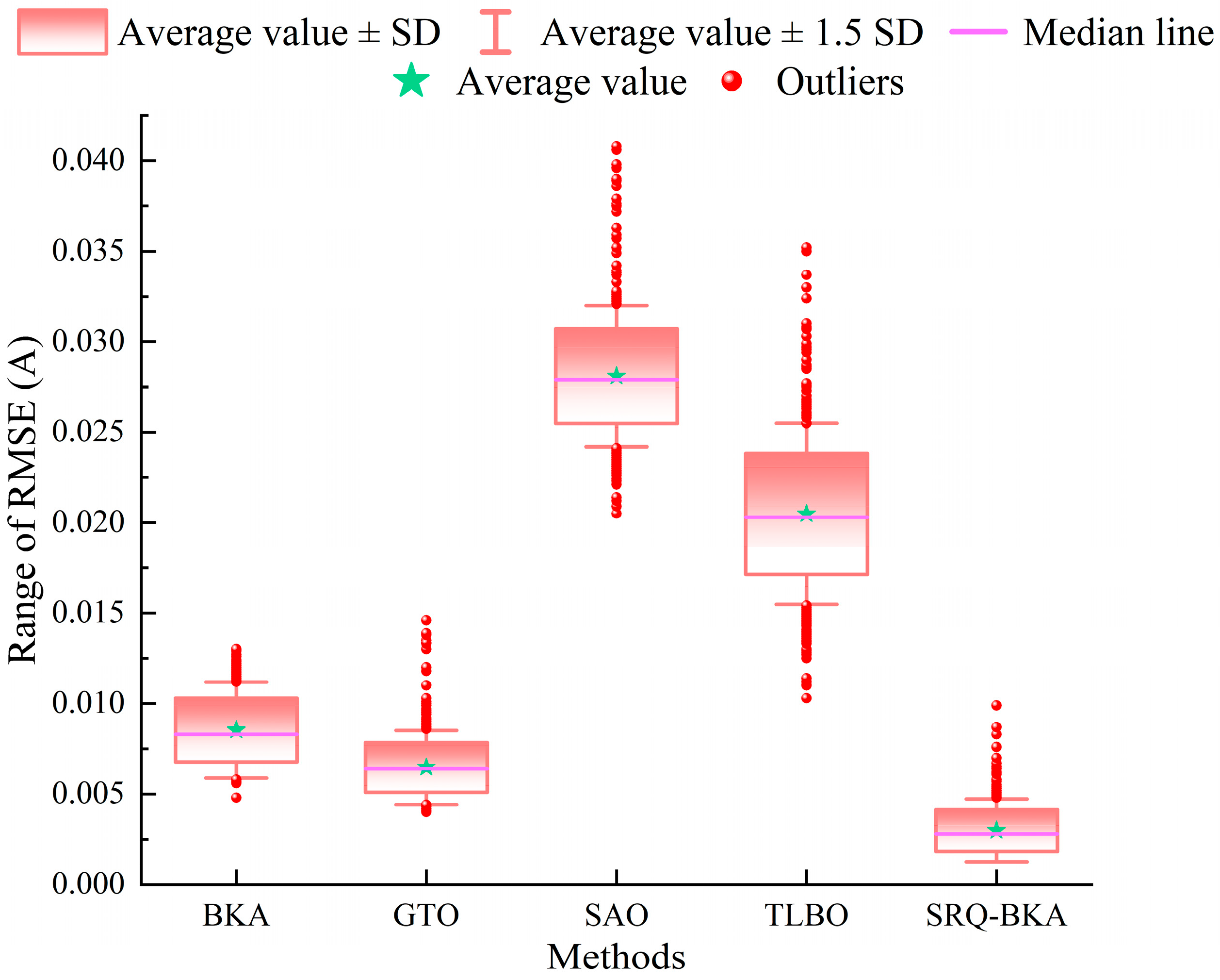
To verify the stability of the proposed method, 1000 repeated experiments were conducted using the BKA, GTO, SAO, TLBO, and SRQ-BKA methods, as they demonstrated relatively strong performance in the previous experiments. The RMSE and C_time for the DDM of the five methods are shown in

Table 12. Average RMSE and C_time of 5 methods after 1000 repeated experiments.

Index	BKA	GTO	SAO	TLBO	SRQ-BKA
RMSE (A)	0.00824	0.00633	0.02790	0.02031	0.00278
Ctime (s)	20.87567	21.15738	21.97542	28.78677	22.44563

. The experiments were repeated 1000 times following the above procedure to further compare the accuracy and stability of the five methods. The average RMSE values for the BKA, GTO, SAO, TLBO, and SRQ-BKA are 0.00824 A, 0.00633 A, 0.02790 A, 0.02031 A, and 0.00278 A, respectively. The SRQ-BKA shows the highest accuracy, followed by GTO and the BKA, and then TLBO and SAO. The average C_time values for these five methods are 20.87567 s, 21.15738 s, 21.97542 s, 28.78677 s, and 22.44563 s, respectively. The variation in C_time among the five methods is minimal and can essentially be neglected.

To provide a more comprehensive evaluation of stability, the standard deviation (SD) and 95% confidence interval (CI) for the RMSE were calculated based on the 1000 trials. As summarized in

Table 13. Standard deviation and 95% confidence interval of RMSE for 5 methods based on 1000 trials.

Method	SD (A)	95% CI of RMSE (A)	Confidence Interval Width
BKA	0.00181	[0.00813, 0.00835]	0.00022
GTO	0.00226	[0.00619, 0.00647]	0.00028
SAO	0.00477	[0.02760, 0.02820]	0.00060
TLBO	0.00566	[0.01996, 0.02067]	0.00071
SRQ-BKA	0.00156	[0.00268, 0.00288]	0.00020

, the SRQ-BKA not only achieves the lowest average RMSE but also exhibits the smallest SD of 0.00156 A and the tightest CI range of [0.00268 A, 0.00288 A], highlighting its superior robustness and repeatability in parameter-identification tasks. These statistical findings are visually reinforced in Figure 11, where the box plot clearly shows that the SRQ-BKA has the narrowest box and the shortest whiskers, with minimal outliers—indicating both high accuracy and strong consistency.

A more detailed comparison of the five methods is shown in Figure 11. The SRQ-BKA box is the most compact, followed by GTO and the BKA, whereas SAO and TLBO exhibit noticeably wider boxes, reflecting greater RMSE variability. The relative positions of the mean and median further confirm the superior parameter identification accuracy of the SRQ-BKA, which is consistent with the earlier experimental results. Additionally, the spread and magnitude of outliers provide further insight into algorithmic stability. The outliers of the SRQ-BKA remain within 0.01 A and those of the BKA and GTO do not exceed 0.015 A, whereas SAO and TLBO exhibit extreme outliers up to 0.035 A, indicating occasional substantial deviations. Overall, the statistical analysis combined with the box-plot visualization confirms that the SRQ-BKA delivers high accuracy along with exceptional robustness and reliability.

Figure 12 presents the C_time box-plot results for the five methods. In Figure 12, the BKA and GTO exhibit relatively short C_time values. TLBO exhibits a slightly longer C_time, and the SRQ-BKA lies between SAO and TLBO. However, the C_time difference between the SRQ-BKA and BKA is less than 2 s. Considering the SRQ-BKA’s advantages in accuracy and stability, this slight time difference does not affect the practical applicability of the parameter-identification method.

4.4. Experiment 3: Comparative Study of Parameter Identification for the SDM, DDM, and TDM

The main PV cell models include the SDM, DDM, and TDM, each with distinct characteristics in terms of computational complexity and accuracy. The SDM has a simple structure and is easy to compute, but its accuracy is relatively low. The TDM, although providing the highest accuracy, is limited in practical application due to its complex computational process. The DDM strikes a good balance between computational accuracy and practicality, particularly in representing I-V characteristics under low-irradiance and high-temperature conditions. In this section, the parameter-identification results of the three models are compared to verify the practicality of the proposed method.

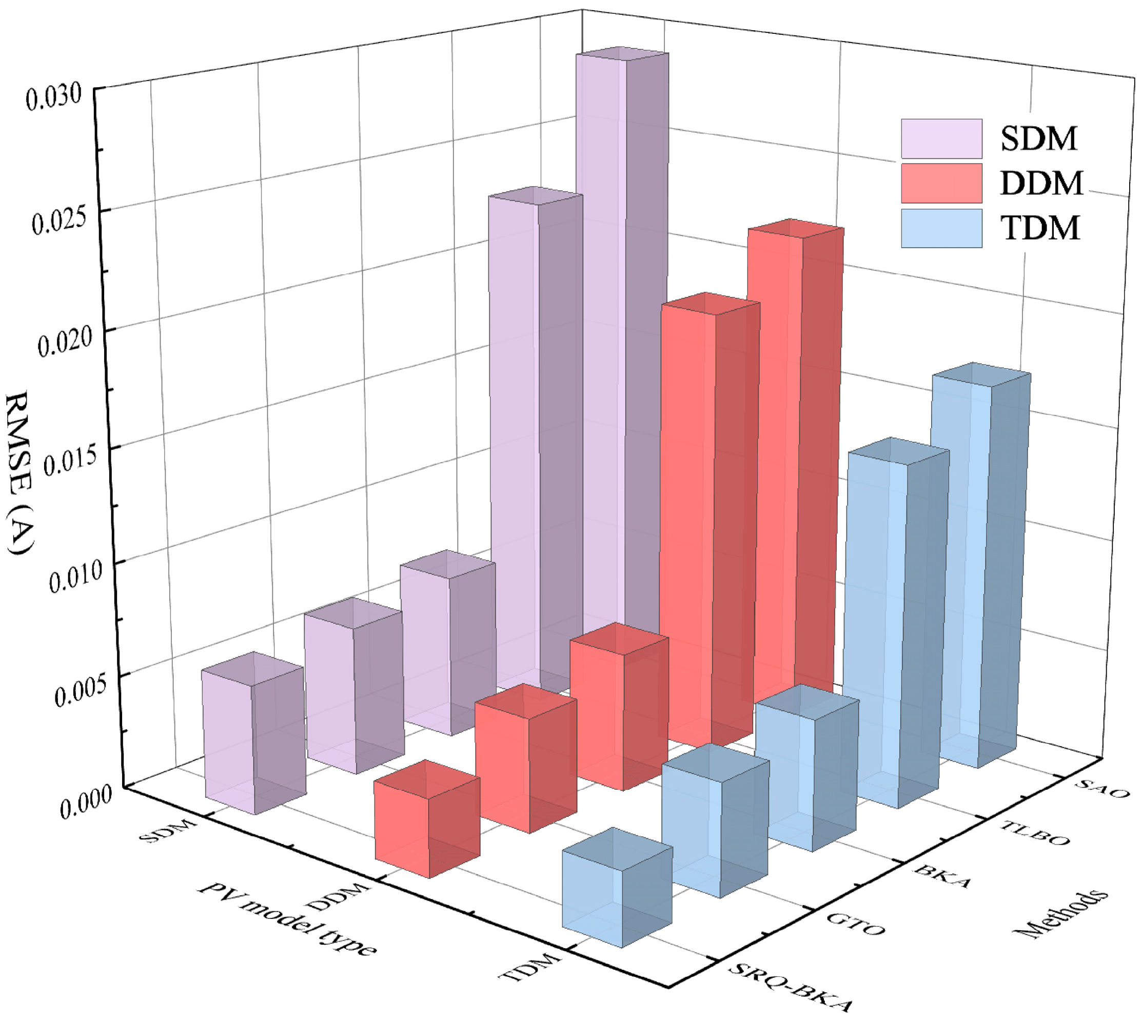
For the TSM-240 PV module, five different methods are applied for parameter identification, and their performance is evaluated based on RMSE.

Table 14. Comparison of RMSE results for five methods applied to the SDM, DDM, and TDM.

Method	RMSE (A)—SDM	RMSE (A)—DDM	RMSE (A)—TDM
BKA	0.00735	0.00613	0.00571
GTO	0.00662	0.00501	0.00487
SAO	0.02878	0.02207	0.01712
TLBO	0.02313	0.01975	0.01503
SRQ-BKA	0.00572	0.00279	0.00266

presents the parameter-identification results for the three models, showing that the SRQ-BKA, GTO, and BKA perform excellently in the SDM, DDM, and TDM parameter identification, outperforming the other methods.

From an overall accuracy perspective, the RMSE of the DDM is lower than that of the SDM, indicating its higher accuracy in PV modeling. Moreover, for the DDM and TDM, the parameter-identification accuracy of the same optimization methods is similar, but the performance of the three leading methods is particularly outstanding.

Figure 13 shows that the RMSE of the SDM is higher than that of the DDM and TDM. For the SRQ-BKA, GTO, and BKA optimization methods, the RMSE values of the DDM and TDM are quite similar. Among these methods, the lowest RMSE value is achieved by the SRQ-BKA. The experiment indicates that the DDM offers an accuracy advantage, along with strong applicability and development potential. Furthermore, the SRQ-BKA demonstrates high accuracy in the SDM, DDM, and TDM, further validating the practicality of the proposed method.

Table 15. Comparison of C_time results for five methods applied to the SDM, DDM, and TDM.

Method	Ctime (s)—SDM	Ctime (s)—DDM	Ctime (s)—TDM
BKA	12.31048	20.12758	31.80107
GTO	11.90859	20.94537	32.95732
SAO	13.58206	21.56345	36.95821
TLBO	15.33927	26.71751	51.96223
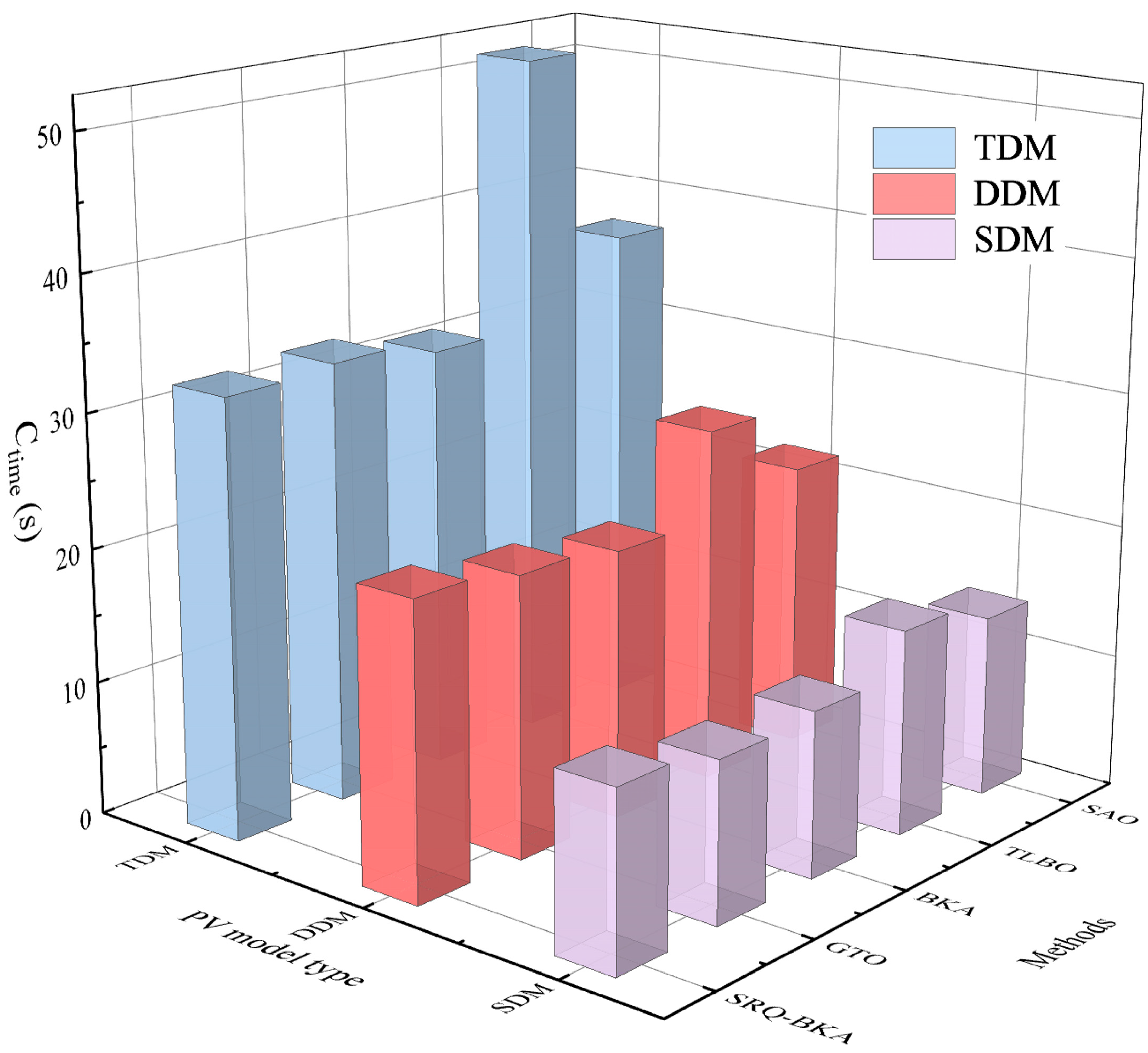
SRQ-BKA	13.15650	21.89987	32.59736

shows the parameter-identification speed of the three models, indicating that the identification speeds of the SRQ-BKA, GTO, and BKA are similar for the corresponding models. Figure 14 illustrates that the C_time for the TDM is higher than that of the DDM and SDM. Within each corresponding diode model, the C_time values of the SRQ-BKA, GTO, and BKA are quite similar. In terms of overall computational cost, the SDM achieves the fastest speed; however, as shown in Figure 13, its identification accuracy is not guaranteed. Moreover, the C_time of the DDM is lower than that of the TDM, indicating that the DDM offers higher efficiency in PV modeling. Specifically, the C_time values of the SRQ-BKA, GTO, and BKA for DDM identification are 21.89987 s, 20.94537 s, and 20.12758 s, which are significantly lower than the corresponding TDM values of 32.59736 s, 32.95732 s, and 31.80107 s.

In conclusion, the DDM exhibits high computational accuracy and strong applicability in PV modeling, particularly achieving the best performance when optimized using the BKA, GTO, and SRQ-BKA. Additionally, the SRQ-BKA method not only fully leverages the theoretical advantages of the DDM but also demonstrates outstanding identification accuracy in the SDM, DDM, and TDM, further confirming its practicality and reliability. As a result, the combination of the DDM with SRQ-BKA optimization holds significant development potential and provides superior solutions for PV-system modeling.

4.5. Discussion

The three experiments conducted in this study comprehensively validate the performance of the proposed SRQ-BKA. In experiment 1, the SRQ-BKA outperforms a range of traditional and modern MAs on benchmark functions, particularly under complex multimodal and noisy conditions, demonstrating superior global optimization and convergence speed. In experiment 2, where the SRQ-BKA is applied for parameter identification of the DDM using real I-V measurements, it achieves the lowest RMSE and the most accurate curve fitting, highlighting its practical effectiveness. Experiment 3 confirms its robustness, as the SRQ-BKA maintains its performance advantage across the SDMs, DDMs, and TDMs, demonstrating its generalizability to different PV model structures.

The outstanding performance of the algorithm is primarily attributed to its hybrid strategy. The SRL mechanism enhances population diversity and prevents premature convergence. The SRS mechanism dynamically adjusts search intensity, effectively balancing exploration and exploitation. The QI mechanism improves local-search precision in the later stages. The integration of these mechanisms leads to higher accuracy, faster convergence, and greater stability compared with existing algorithms.

According to the experimental results, the SRQ-BKA consistently excels in handling complex multimodal problems, real-world PV model identification, and various PV model structures. The combination of SRL, SRS, and QI enhances its global-search ability, local precision, and convergence speed, making it a highly effective optimization method.

In addition to its optimization performance, the SRQ-BKA exhibits desirable characteristics for practical deployment in PV systems. As a population-based algorithm, the fitness evaluations of individuals within each iteration are mutually independent, which enables efficient parallel implementation using multi-threading or GPU acceleration. Moreover, the algorithm maintains a fixed iteration count and employs lightweight enhancement mechanisms, making it suitable for near real-time applications such as online parameter estimation and fault detection in PV systems, without imposing significant computational overhead.

5. Conclusions

This research addresses the engineering challenge of PV model parameter identification by proposing an improved Black-Winged Kite Algorithm (SRQ-BKA). The method enhances parameter identification accuracy through key improvements in initialization, optimization, and convergence. The SRL mechanism replaces traditional random initialization, improving the quality of the parameter distribution. A dynamic search strategy based on SRS adapts the search step size, effectively balancing global exploration and local refinement. Additionally, the QI mechanism accelerates convergence and further refines the solution. In the TSM-240 module test, the SRQ-BKA achieves a significant improvement, reducing the final RMSE to 0.00262A.

The SRQ-BKA outperforms the BKA, GTO, GWO, SAO, RIME, DE, GA, and TLBO in convergence accuracy and speed across benchmark functions F5, F7, and F10. In the F5 test, the SRQ-BKA accurately reaches the global optimum. In the noisy F7 function, it improves accuracy by 47% and speeds up by 39% compared with GTO. For the multimodal F10 function, the SRQ-BKA achieves the optimal value in 27 iterations, which is 120 fewer than the BKA. These results demonstrate the outstanding potential of the SRQ-BKA in PV model parameter identification. It also excels in identifying parameters under various environmental conditions. At 379 W/m² irradiance and 27.9 °C temperature, the SRQ-BKA achieves the lowest RMSE of 0.00262 A. Even at a higher irradiance of 900 W/m² and temperature of 47.8 °C, the RMSE remains low at 0.00823 A, with an R² greater than 0.99998, indicating excellent accuracy. The P-V curve closely matches the measured data, confirming the algorithm’s reliability. In 1000 repeated experiments, the RMSE range for the SRQ-BKA is from 0.00184 to 0.00422, significantly outperforming comparison algorithms, showcasing its stability. Additionally, the SRQ-BKA demonstrates versatility in parameter identification for the SDM, DDM, and TDM. For the DDM, the SRQ-BKA achieves an RMSE of 0.00279 A and a C_time of 21.90 s, improving speed by nearly 35% compared to the TDM while maintaining similar accuracy.

Although the proposed SRQ-BKA demonstrates high accuracy and robustness in both benchmark evaluations and real-world photovoltaic system experiments, certain limitations persist. The algorithm is sensitive to environmental disturbances, particularly under rapidly fluctuating irradiance and temperature conditions, which may lead to performance variability. Moreover, its dependence on high-quality, representative I-V datasets make it susceptible to degraded identification accuracy when the data are noisy or incomplete. In response to these limitations, future research will focus on developing enhanced noise-resilient mechanisms, implementing real-time online parameter identification for PV modules, and systematically evaluating the algorithm’s adaptability and stability under extreme climatic conditions.

References

1. Hao, D.; Qi, L.; Tairab, A.M.; Ahmed, A.; Azam, A.; Luo, D.; Pan, Y.; Zhang, Z.; Yan, J. Solar Energy Harvesting Technologies for PV Self-Powered Applications: A Comprehensive Review. Renew. Energy 2022, 188, 678–697. [Google Scholar] [CrossRef]
2. Amiri, A.F.; Oudira, H.; Chouder, A.; Kichou, S. Faults Detection and Diagnosis of PV Systems Based on Machine Learning Approach Using Random Forest Classifier. Energy Convers. Manag. 2024, 301, 118076. [Google Scholar] [CrossRef]
3. Oliva, D.; Elaziz, M.A.; Elsheikh, A.H.; Ewees, A.A. A Review on Meta-Heuristics Methods for Estimating Parameters of Solar Cells. J. Power Sources 2019, 435, 126683. [Google Scholar] [CrossRef]
4. Siddiqui, M.U.; Siddiqui, O.K.; Alquaity, A.B.S.; Ali, H.; Arif, A.F.M.; Zubair, S.M. A Comprehensive Review on Multi-Physics Modeling of Photovoltaic Modules. Energy Convers. Manag. 2022, 258, 115414. [Google Scholar] [CrossRef]
5. Chenouard, R.; El-Sehiemy, R.A. An Interval Branch and Bound Global Optimization Algorithm for Parameter Estimation of Three Photovoltaic Models. Energy Convers. Manag. 2020, 205, 112400. [Google Scholar] [CrossRef]
6. Venkateswari, R.; Rajasekar, N. Review on Parameter Estimation Techniques of Solar Photovoltaic Systems. Int. Trans. Electr. Energ. Syst. 2021, 31, e13113. [Google Scholar] [CrossRef]
7. Ridha, H.M.; Hizam, H.; Gomes, C.; Heidari, A.A.; Chen, H.; Ahmadipour, M.; Muhsen, D.H.; Alghrairi, M. Parameters Extraction of Three Diode Photovoltaic Models Using Boosted LSHADE Algorithm and Newton Raphson Method. Energy 2021, 224, 120136. [Google Scholar] [CrossRef]
8. Zhou, W.; Wang, P.; Heidari, A.A.; Zhao, X.; Turabieh, H.; Mafarja, M.; Chen, H. Metaphor-Free Dynamic Spherical Evolution for Parameter Estimation of Photovoltaic Modules. Energy Rep. 2021, 7, 5175–5202. [Google Scholar] [CrossRef]
9. Restrepo-Cuestas, B.J. Bishop Model Parameter Estimation in Photovoltaic Cells Using Metaheuristic Optimization Techniques. Sol. Energy 2024, 270, 112410. [Google Scholar] [CrossRef]
10. Lai, V.; Huang, Y.F.; Koo, C.H.; Ahmed, A.N.; El-Shafie, A. A Review of Reservoir Operation Optimisations: From Traditional Models to Metaheuristic Algorithms. Arch. Comput. Methods Eng. 2022, 29, 3435–3457. [Google Scholar] [CrossRef] [PubMed]
11. Song, E.; Yao, Z.; Wang, Z. A Dynamic Multi-Objective Differential Evolution Based on Hierarchical Prediction Strategy. In Proceedings of the 2024 6th International Conference on Data-driven Optimization of Complex Systems (DOCS), Hangzhou, China, 16–18 August 2024; pp. 761–766. [Google Scholar]
12. Chun, Y.; Hua, X.; Qi, C.; Yao, Y.X. Improved Marine Predators Algorithm for Engineering Design Optimization Problems. Sci. Rep. 2024, 14, 13000. [Google Scholar] [CrossRef]
13. Faramarzi, A.; Heidarinejad, M.; Stephens, B.; Mirjalili, S. Equilibrium Optimizer: A Novel Optimization Algorithm. Knowl. Based Syst. 2020, 191, 105190. [Google Scholar] [CrossRef]
14. Hammadi, W.Q.; Qasim, O.S. Hybrid Binary Atom Search Optimization Approaches with Statistical Dependence for Feature Selection. In Proceedings of the 2022 International Conference on Computer Science and Software Engineering (CSASE), Duhok, Iraq, 15–17 March 2022; pp. 218–223. [Google Scholar]
15. Deng, L.; Liu, S. Snow Ablation Optimizer: A Novel Metaheuristic Technique for Numerical Optimization and Engineering Design. Expert. Syst. Appl. 2023, 225, 120069. [Google Scholar] [CrossRef]
16. Su, H.; Zhao, D.; Heidari, A.A.; Liu, L.; Zhang, X.; Mafarja, M.; Chen, H. RIME: A Physics-Based Optimization. Neurocomputing 2023, 532, 183–214. [Google Scholar] [CrossRef]
17. Chen, X.; Yu, K.; Du, W.; Zhao, W.; Liu, G. Parameters Identification of Solar Cell Models Using Generalized Oppositional Teaching Learning Based Optimization. Energy 2016, 99, 170–180. [Google Scholar] [CrossRef]
18. Bayzidi, H.; Talatahari, S.; Saraee, M.; Lamarche, C.-P. Social Network Search for Solving Engineering Optimization Problems. Comput. Intell. Neurosci. 2021, 2021, 8548639. [Google Scholar] [CrossRef] [PubMed]
19. Feng, Z.; Niu, W.; Liu, S. Cooperation Search Algorithm: A Novel Metaheuristic Evolutionary Intelligence Algorithm for Numerical Optimization and Engineering Optimization Problems. Appl. Soft Comput. 2021, 98, 106734. [Google Scholar] [CrossRef]
20. Fan, Y.; Wang, P.; Heidari, A.A.; Chen, H.; HamzaTurabieh; Mafarja, M. Random Reselection Particle Swarm Optimization for Optimal Design of Solar Photovoltaic Modules. Energy 2022, 239, 121865. [Google Scholar] [CrossRef]
21. Mirjalili, S.; Lewis, A. The Whale Optimization Algorithm. Adv. Eng. Softw. 2016, 95, 51–67. [Google Scholar] [CrossRef]
22. Makhadmeh, S.N.; Al-Betar, M.A.; Doush, I.A.; Awadallah, M.A.; Kassaymeh, S.; Mirjalili, S.; Zitar, R.A. Recent Advances in Grey Wolf Optimizer, Its Versions and Applications: Review. IEEE Access 2024, 12, 22991–23028. [Google Scholar] [CrossRef]
23. Wang, J.; Wang, W.; Hu, X.; Qiu, L.; Zang, H. Black-Winged Kite Algorithm: A Nature-Inspired Meta-Heuristic for Solving Benchmark Functions and Engineering Problems. Artif. Intell. Rev. 2024, 57, 98. [Google Scholar] [CrossRef]
24. Chen, X.; Ding, K.; Zhang, J.; Yang, Z.; Liu, Y.; Yang, H. A Two-Stage Method for Model Parameter Identification Based on the Maximum Power Matching and Improved Flow Direction Algorithm. Energy Convers. Manag. 2023, 278, 116712. [Google Scholar] [CrossRef]
25. Jiang, M.; Ding, K.; Chen, X.; Cui, L.; Zhang, J.; Cang, Y.; Yang, H.; Gao, R. CGH-GTO Method for Model Parameter Identification Based on Improved Grey Wolf Optimizer, Honey Badger Algorithm, and Gorilla Troops Optimizer. Energy 2024, 296, 131163. [Google Scholar] [CrossRef]
26. Chen, X.; Xu, B.; Mei, C.; Ding, Y.; Li, K. Teaching–Learning–Based Artificial Bee Colony for Solar Photovoltaic Parameter Estimation. Appl. Energy 2018, 212, 1578–1588. [Google Scholar] [CrossRef]
27. Long, W.; Cai, S.; Jiao, J.; Xu, M.; Wu, T. A New Hybrid Algorithm Based on Grey Wolf Optimizer and Cuckoo Search for Parameter Extraction of Solar Photovoltaic Models. Energy Convers. Manag. 2020, 203, 112243. [Google Scholar] [CrossRef]
28. Alsaggaf, W.; Gafar, M.; Sarhan, S.; Shaheen, A.M.; Ginidi, A.R. Chemical-Inspired Material Generation Algorithm (MGA) of Single- and Double-Diode Model Parameter Determination for Multi-Crystalline Silicon Solar Cells. Appl. Sci. 2024, 14, 8549. [Google Scholar] [CrossRef]
29. Hakmi, S.H.; Alnami, H.; Moustafa, G.; Ginidi, A.R.; Shaheen, A.M. Modified Rime-Ice Growth Optimizer with Polynomial Differential Learning Operator for Single- and Double-Diode PV Parameter Estimation Problem. Electronics 2024, 13, 1611. [Google Scholar] [CrossRef]
30. Qian, Z.; Zhang, Y.; Pu, D.; Xie, G.; Pu, D.; Ye, M. A New Hybrid Improved Kepler Optimization Algorithm Based on Multi-Strategy Fusion and Its Applications. Mathematics 2025, 13, 405. [Google Scholar] [CrossRef]
31. González, I.; Portalo, J.M.; Calderón, A.J. Configurable IoT Open-Source Hardware and Software I-V Curve Tracer for Photovoltaic Generators. Sensors 2021, 21, 7650. [Google Scholar] [CrossRef] [PubMed]
32. Ashraf, H.; Draz, A.; Elmoaty, A.M.; El-Fergany, A.A. Precise Modelling of Commercial Photovoltaic Cells/Modules of Different Technologies Using Hippopotamus Optimizer. Energy Convers. Manag. 2025, 325, 119382. [Google Scholar] [CrossRef]
33. Oulcaid, M.; El Fadil, H.; Ammeh, L.; Yahya, A.; Giri, F. Parameter Extraction of Photovoltaic Cell and Module: Analysis and Discussion of Various Combinations and Test Cases. Sustain. Energy Technol. Assess. 2020, 40, 100736. [Google Scholar] [CrossRef]
34. Zhang, J.; Liu, Y.; Li, Y.; Ding, K.; Feng, L.; Chen, X.; Chen, X.; Wu, J. A Reinforcement Learning Based Approach for On-Line Adaptive Parameter Extraction of Photovoltaic Array Models. Energy Convers. Manag. 2020, 214, 112875. [Google Scholar] [CrossRef]
35. Yang, X.; Zeng, G.; Cao, Z.; Huang, X.; Zhao, J. Parameters Estimation of Complex Solar Photovoltaic Models Using Bi-Parameter Coordinated Updating L-SHADE with Parameter Decomposition Method. Case Stud. Therm. Eng. 2024, 61, 104917. [Google Scholar] [CrossRef]
36. Zhang, Y. Backtracking Search Algorithm with Specular Reflection Learning for Global Optimization. Knowl. Based Syst. 2021, 212, 106546. [Google Scholar] [CrossRef]
37. Qaraad, M.; Amjad, S.; Hussein, N.K.; Farag, M.A.; Mirjalili, S.; Elhosseini, M.A. Quadratic Interpolation and a New Local Search Approach to Improve Particle Swarm Optimization: Solar Photovoltaic Parameter Estimation. Expert. Syst. Appl. 2024, 236, 121417. [Google Scholar] [CrossRef]
38. Jiang, M.; Ding, K.; Chen, X.; Cui, L.; Zhang, J.; Yang, Z.; Cang, Y.; Cao, S. Research on Time-Series Based and Similarity Search Based Methods for PV Power Prediction. Energy Convers. Manag. 2024, 308, 118391. [Google Scholar] [CrossRef]
Figure 1. Framework of the proposed method for seven-model parameter identification.
Machines 13 00706 g001
Figure 2. Process of the SRQ-BKA.
Machines 13 00706 g002
Figure 3. Equivalent circuit of double diode model (DDM).
Machines 13 00706 g003
Figure 4. Visual distribution of random, OBL, and SRL.
Machines 13 00706 g004
Figure 5. I-V curve and ambient parameter measurement system.
Machines 13 00706 g005
Figure 6. Iteration optimization search curves of different MAs: (a) F5; (b) F7; (c) F10.
Machines 13 00706 g006
Figure 7. Comparison of model parameter identification results for 9 methods under environmental conditions (379 W/m2, 27.9 °C): (a) 2D iteration curve, (b) 3D iteration curve, (c) I-V curve, (d) P-V curve.
Machines 13 00706 g007
Figure 8. Comparison of model parameter identification results for 9 methods under environmental conditions (590 W/m2, 36.5 °C): (a) 2D iteration curve, (b) 3D iteration curve, (c) I-V curve, (d) P-V curve.
Machines 13 00706 g008
Figure 9. Comparison of model parameter identification results for 9 methods under environmental conditions (900 W/m2, 47.8 °C): (a) 2D iteration curve, (b) 3D iteration curve, (c) I-V curve, (d) P-V curve.
Machines 13 00706 g009
Figure 10. Comparison of evaluation metrics for model parameter identification results of different methods: (a) MAE, (b) MAPE, (c) R2, (d) RMSE, (e) Ctime.
Machines 13 00706 g010
Figure 11. RMSE box plot of 1000 repetition experiments for five methods.
Machines 13 00706 g011
Figure 12. Ctime box plot of 1000 repetition experiments for five methods.
Machines 13 00706 g012
Figure 13. RMSE comparison for SDM, DDM, and TDM parameter identification.
Machines 13 00706 g013
Figure 14. Ctime comparison for SDM, DDM, and TDM parameter identification.
Machines 13 00706 g014