Abstract
Accurate estimation of the vehicle sideslip angle is critical for the effective operation of advanced driver assistance systems and active safety functions such as electronic stability control. However, direct measurement of sideslip angle is impractical in series-production vehicles due to high sensor cost. Furthermore, existing estimation methods often neglect the impact of model uncertainties on estimation error, which can compromise estimation reliability and, consequently, vehicle stability. To address these limitations, this paper proposes an interval observer based on a Kalman filter that accounts explicitly for model uncertainties in the sideslip angle estimation process. The proposed method generates both upper and lower bounds of the estimated sideslip angle, providing a quantifiable measure of uncertainty that enhances the robustness of control systems that depend on this measurement. Given the limitations of simplified vehicle models, a combined vehicle roll and lateral dynamics model is utilized to improve estimation accuracy. The effectiveness of the proposed methodology is demonstrated through a series of simulation experiments conducted using CarSim.
1. Introduction
Since the early 1990s, when electronic stability control (ESC) and other onboard active systems were first introduced to manage vehicle dynamics, accurately estimating the vehicle sideslip angle has remained a complex and critical challenge [1,2,3,4,5,6].
Today’s advanced vehicle control technologies, such as rear-wheel steering [7,8], active front steering [9,10], direct yaw moment control [11,12], and torque vectoring [13,14], are increasingly integrated to push the limits of vehicle performance and stability. These systems work together to significantly improve key aspects of driving, including road-holding, cornering performance, handling responsiveness, and overall dynamic behavior. Their importance becomes even more pronounced during sudden maneuvers or when driving on low-friction surfaces, where the driver’s ability to maintain control is most compromised [15]. The performance of these sophisticated control systems depends on precise, real-time information about the vehicle’s dynamic state [16,17,18], with the sideslip angle being one of the most important parameters [19]. Accurate estimation of this angle is essential for the success of active safety features, as it directly influences the vehicle’s ability to avoid dangerous situations such as rollover [20].
From a mechanical perspective, the sideslip angle is affected by variables such as lateral acceleration, the vehicle’s mass and how it is distributed, along with the rear axle’s slip angle [21]. Pneumatic tires, in particular, are known to have a nonlinear response between lateral force and slip angle, largely due to phenomena like saturation and sensitivity to vertical load [22]. Therefore, it is necessary for vehicle control systems to respond quickly when instability can occur. These systems are primarily designed to act early, ensuring that lateral forces remain within limits that prevent the tires from entering their nonlinear saturation zone. This is an operating state associated with a significant loss of lateral grip and an increased risk of skidding or directional instability. The issue becomes even more critical under low-friction conditions, where tire saturation will occur at much smaller slip angles [23].
In the field of vehicle dynamics, it is well-known that directly measuring the sideslip angle in series-production vehicles is not feasible [24,25,26]. Unlike variables such as lateral acceleration or yaw rate (which can be monitored using affordable and widely available sensors like IMUs), sideslip angle measurement requires advanced equipment, such as optical ground speed sensors [27] or dual-GPS antennas with high resolution [28]. These systems are typically limited to research and development purposes due to major drawbacks, such as their high cost, installation complexity, limited durability, and long-term reliability. These limitations highlight the need to develop accurate and reliable sideslip angle estimation algorithms that can support ESC.
A variety of methods have been proposed for estimating the sideslip angle, yet no single approach has proven to be universally accurate or dependable under all driving scenarios. Within the mechanical and automotive engineering communities, there is a clear preference for model-based estimation techniques, which utilize a predefined vehicle model to guide the design of state observers [29,30]. In [31], an algorithm that estimates the sideslip angle by combining dynamic and kinematic vehicle models without requiring supplementary sensors is presented. In [32], a cost-effective method to jointly estimate the vehicle sideslip angle and lateral tire–road forces is introduced, only requiring the information from onboard sensors, readily available on mass-production vehicles. In [33], a robust adaptive filtering estimator is used for the joint estimation of vehicle sideslip angle and tire–road forces. In [34], an event-triggered fuzzy filtering for vehicle sideslip angle estimation with consideration of data quantization and dropouts is presented. However, it is important to highlight that the previously mentioned studies do not incorporate model uncertainties into the sideslip angle estimation process, so they overlook the inherent uncertainty associated with the estimated sideslip angle. Once a value has been estimated, a significant estimation error can adversely affect vehicle stability, particularly when the estimate is used as an input to vehicle control systems [35]. Inaccurate inputs may lead to suboptimal or incorrect control actions, thereby increasing the risk of instability [36].
In response to the aforementioned challenges, this work introduces an interval observer based on a Kalman filter to estimate the vehicle’s sideslip angle while explicitly accounting for model uncertainties. Unlike conventional methods, the proposed approach provides both upper and lower bounds on the estimated sideslip angle, offering a quantifiable measure of estimation uncertainty and improving the reliability of inputs to vehicle control systems. Recognizing that a bicycle model lacks the fidelity required to accurately capture vehicle dynamics, a combined roll and lateral dynamics model is employed instead. To evaluate the effectiveness of the proposed methodology, a series of simulation tests are conducted using CarSim.
2. Vehicle Model
This chapter presents the vehicle dynamics model employed for sideslip angle estimation. In order to design an observer that estimates the sideslip angle, both lateral and roll dynamics of the vehicle are considered, since these are heavily coupled [37]. The vehicle model (see Figure 1) has three degrees of freedom, i.e., the sideslip angle , the yaw rate r, and the roll angle . The vehicle parameters are given in Table 1.
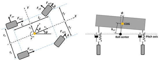
Figure 1.
Vehicle roll and lateral dynamics model [20].

Table 1.
Vehicle parameters and variables.
Assuming small angles and slow vehicle speed variation, the vehicle dynamics are expressed as follows [37]:
Given that the vehicle’s roll center does not coincide with its center of gravity, it is necessary to recalculate the moment of inertia with respect to the roll center using Steiner’s theorem (the parallel axis theorem). Accordingly, the equivalent moment of inertia, , is determined by transforming the known moment of inertia about the center of gravity to the roll center reference frame.
Due to the inherently nonlinear dynamics of the vehicle, a Linear Parameter-Varying (LPV) continuous-time state-space model is employed in this work. Accordingly, (1) is formulated as
where is the state vector and is the control input, where is the steering angle. In this work, we assume that the yaw rate, roll angle, and roll rate can be measured by an inertial measurement unit (IMU). Hence, the measurement vector is defined as . Additionally, the longitudinal velocity can be measured using wheel speed sensors. The state-space matrices of the system (2) are
A key limitation of the model (2) lies in the inherently complex and nonlinear behavior of tire dynamics. Specifically, the matrices and depend on the time-varying vehicle speed. Furthermore, the front and rear cornering stiffnesses are not constant but vary over time in response to changing driving conditions and road surface characteristics [38]. Moreover, accurately estimating their instantaneous values in real time is highly challenging [39,40,41]. To address this, it is assumed that these parameters remain bounded within known limits throughout the vehicle’s operation, such that
The presence of model uncertainties, particularly in tire parameters, compromises the accuracy of state estimations for variables that are not directly measurable, such as the sideslip angle. To mitigate this issue, the subsequent section introduces an interval observer capable of estimating bounded intervals within which the sideslip angle is guaranteed to lie at each time instant. This approach enhances robustness against parameter variability and modeling inaccuracies.
3. Interval Kalman Filter
3.1. Preliminaries
In order to ease real-time implementation, the continuous-time system (2) is converted into its discrete-time counterpart using Euler’s method [42]:
which leads to the discrete-time state-space model:
It is clear that T is the sampling period, denotes the value of the state x at the k instant, and indicates dependency on the time-varying vector . The state-space matrices of (5) are given by
Since can be measured online but and cannot be, it is possible to express system (5) as the convex sum
where
It is then assumed that the actual behavior of the vehicle will be contained within four different subsystems, , each with their own states, , and different sets of state-space matrices, , that depend on the limits of unmeasurable uncertain parameters, such that
Then, the current states of the real system are assumed to be contained within the interval
3.2. Extended Kalman Filter
Following the presentation of each subsystem, , the next step is to design a filter for estimating the sideslip angle in each case. Given that the system matrices evolve over time as a function of the longitudinal velocity , an Extended Kalman Filter (EKF) is selected to effectively handle the system’s inherent nonlinearity and time-varying behavior [43].
Although the Kalman filter can be expressed as a single recursive equation, it is generally considered to have two distinct stages: prediction and correction [44]. During the prediction phase, the filter uses the previous state estimate to forecast the system’s state at the current time step. This prediction, referred to as the a priori estimate, represents the anticipated state before incorporating any new measurement data. In the correction (or update) phase, the filter adjusts this prediction by evaluating the innovation, the discrepancy between the predicted measurement, and the actual observation. This difference is weighted by the Kalman gain, which is computed to minimize estimation error. The result is an improved state estimate, known as the a posteriori estimate, which integrates both the model prediction and the latest measurement. The two stages of our EKF are formulated as follows [45]:
- Predict.
- Update.Matrices P, Q, and R denote the prediction, process noise, and observation noise covariances, respectively. Since Q and R are constant, these do not have time indices.
Based on the minimum and maximum estimated values of the system states at each time instant, denoted by (, ), the corresponding interval in which the real sideslip angle of the vehicle may be contained is
4. Results
To validate the proposed sideslip angle estimator, a comprehensive set of simulations was performed using the vehicle dynamics software CarSim. CarSim is a high-fidelity vehicle dynamics simulation software that has gained significant popularity in both industry and academia for its ability to model and analyze the behavior of ground vehicles. The model provides detailed physical representations of key subsystems, including suspension, steering, tires, brakes, and powertrain. These components enable the accurate representation of vehicle dynamics under various driving conditions. In this work, CarSim is co-simulated with MATLAB/Simulink using the CarSim–Simulink interface. The architecture of the proposed methodology is illustrated in Figure 2. The evaluation focused on two test scenarios: a double lane change maneuver and a racetrack. For the purpose of comparative analysis, the accuracy of the estimator was benchmarked against an estimator designed under a conventional bicycle model (also known as single-track model) [46], since this approach simplifies the vehicle’s lateral dynamics by neglecting the influence of roll dynamics. In the simulations, the vehicle starts at a desired constant speed, without the need for an acceleration or braking phase. Given that no speed controller was implemented to adapt the vehicle’s velocity to the curvature of the path, CarSim was configured to maintain a fixed target speed throughout the maneuver.
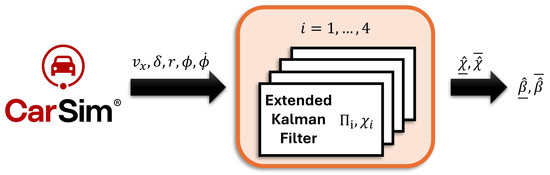
Figure 2.
Proposed interval observer architecture.
By trial and error, the Kalman matrices are defined as follows:
4.1. Double Lane Change Test
The double lane change is a common maneuver encountered in everyday driving [47,48,49], typically performed to overtake slower vehicles or to avoid unexpected obstacles on the road. This maneuver involves abrupt lateral movements, which can significantly affect the vehicle’s lateral dynamics. Specifically, the sideslip angle increases in response to a sudden rise in lateral velocity. This effect can compromise vehicle stability and control, especially at higher speeds. Consequently, continuous monitoring of the sideslip angle in this particular scenario is essential to assess vehicle safety and ensure that the maneuver remains within controllable limits.
The configuration and main results of this scenario are depicted in Figure 3. As longitudinal velocity is not expected to vary significantly during the maneuver, it was maintained at a constant 50 km/h. The steering input was defined as a symmetrical sinusoidal signal to ensure the vehicle returns to its original lane without lateral offset. The sideslip angle and roll angle exhibit remarkably similar patterns, reflecting the strong coupling between lateral and roll dynamics in a vehicle. This close relationship highlights the importance of using a comprehensive vehicle model that simultaneously incorporates both lateral and roll dynamics to accurately estimate the sideslip angle, which will be further demonstrated.
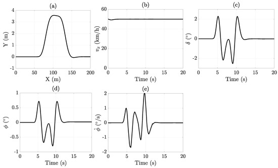
Figure 3.
DLC maneuver results: (a) X-Y position, (b) longitudinal velocity, (c) steering angle, (d) roll angle, and (e) roll rate.
Figure 4 illustrates the sideslip angle estimation using an interval observer based on a Kalman filter. The results clearly show that employing a more sophisticated vehicle model significantly enhances the accuracy of the state estimation. Specifically, the root mean square (RMS) estimation error decreased from 0.1171 when using a basic bicycle model to 0.0376 with the integrated lateral and roll dynamics model, highlighting the value of a more extensive modeling approach. The uncertainty area, calculated as the integral of the uncertainty envelope (sum of absolute errors), is presented as an indicator to evaluate the quality of the interval observer:
In this scenario, the uncertainty area calculated using the bicycle model was 6.09°s, whereas the integrated lateral and roll dynamics model reduced this value significantly to 0.91°s, clearly demonstrating a marked improvement in estimation accuracy.
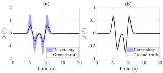
Figure 4.
Sideslip angle estimation during the DLC test: (a) bicycle model only; (b) bicycle model + roll dynamics.
4.2. Racetrack Test
The configuration and main results of this scenario are depicted in Figure 5. This racetrack scenario, generated using CarSim, is widely adopted by researchers as a standardized benchmark for vehicle dynamics validation. The racetrack provides a realistic and challenging environment that tests the performance and robustness of vehicle models.
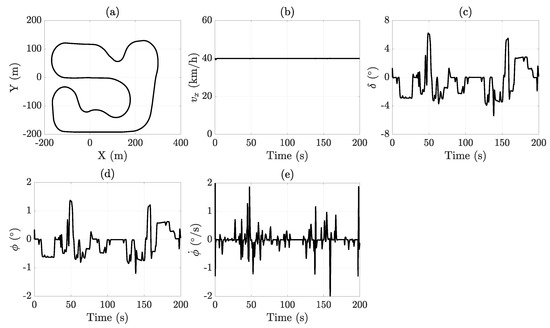
Figure 5.
Racetrack maneuver results: (a) X-Y position, (b) longitudinal velocity, (c) steering angle, (d) roll angle, and (e) roll rate.
As shown in Figure 6, the sideslip angle estimation during the racetrack test exhibits a clear improvement with increasing model complexity. The simpler bicycle model produces noticeable errors in tracking the sideslip angle, whereas the integrated lateral and roll dynamics model closely matches the actual values throughout diverse maneuvers. The RMS estimation error is significantly reduced, dropping from 0.15°
when using the bicycle model to just 0.05° with the integrated lateral and roll dynamics model. Similarly, the uncertainty area decreases from 106.49°s with the bicycle model to 22.65°s when employing the more comprehensive integrated model. This finding emphasizes the efficacy of employing a more sophisticated vehicle model to achieve more precise and reliable state estimation under dynamic driving conditions.
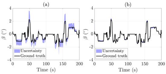
Figure 6.
Sideslip angle estimation during the racetrack test: (a) bicycle model only; (b) bicycle model + roll dynamics.
Table 2 provides a summary of the simulation results regarding the sideslip angle estimation simulation.
Table 2.
Summary of sideslip angle estimation results for two vehicle dynamic models. RMS denotes the root mean square error of the estimated sideslip angle, and denotes the absolute error area over time. Lower values indicate better performance.
5. Conclusions
This work presents an interval observer for vehicle sideslip angle estimation, built on a Kalman filter framework and explicitly accounting for model uncertainties. Instead of providing a single estimate, the observer delivers upper and lower bounds on the sideslip angle, offering a quantifiable measure of uncertainty. This enhances the reliability of inputs for vehicle control systems such as ESC. In contrast to traditional approaches that rely on overly simplified models, this study employs a combined roll and lateral dynamics model, resulting in more accurate estimations across a broader range of driving conditions.
Simulation tests conducted in CarSim demonstrated the effectiveness of the proposed observer in capturing sideslip angle behavior while maintaining robustness to model uncertainties. These results highlight the potential of the method to enhance the performance and safety of vehicle control systems, particularly in situations where direct measurement is infeasible and estimation reliability is critical.
Future work will focus on experimental validation through vehicle testing to analyze the practical applicability and real-time performance of the proposed method under real-world driving conditions. Additionally, the estimated sideslip angle will be used as an input for path/trajectory tracking controllers [50,51,52,53,54].
Author Contributions
Conceptualization, F.V.-M., M.M.-U., B.L. and B.L.B.; methodology, F.V.-M.; software, F.V.-M.; validation, F.V.-M., M.M.-U., B.L. and B.L.B.; formal analysis, F.V.-M.; investigation, F.V.-M.; resources, F.V.-M.; data curation, F.V.-M.; writing—original draft preparation, F.V.-M.; writing—review and editing, F.V.-M., M.M.-U., B.L. and B.L.B.; visualization, F.V.-M.; supervision, B.L.B.; project administration, F.V.-M.; funding acquisition, F.V.-M. and B.L.B. All authors have read and agreed to the published version of the manuscript.
Funding
This work was supported in part by UC3M’s grants for young doctors (Grant No. 2024/00741/001) and by the grant [PID2022-136468OB-I00] funded by MCIN/AEI/10.13039/501100011033, and by “ERDF A way of making Europe”.
Institutional Review Board Statement
Not applicable.
Informed Consent Statement
Not applicable.
Data Availability Statement
The original contributions presented in the study are included in the article; further inquiries can be directed to the corresponding author.
Conflicts of Interest
The authors declare no conflicts of interest.
Abbreviations
The following abbreviations are used in this manuscript:
| ESC | Electronic stability control |
| EKF | Extended Kalman Filter |
| IMU | Inertial measurement unit |
| LPV | Linear Parameter-Varying |
| RMS | Root mean square |
References
- Farmer, C.M. Effect of electronic stability control on automobile crash risk. Traffic Inj. Prev. 2004, 5, 317–325. [Google Scholar] [CrossRef]
- Liebemann, E.; Meder, K.; Schuh, J.; Nenninger, G. Safety and Performance Enhancement: The Bosch Electronic Stability Control (ESP); Technical Report, SAE Technical Paper; SAE: Warrendale, PA, USA, 2004. [Google Scholar]
- Chindamo, D.; Lenzo, B.; Gadola, M. On the vehicle sideslip angle estimation: A literature review of methods, models, and innovations. Appl. Sci. 2018, 8, 355. [Google Scholar] [CrossRef]
- Jin, X.; Yin, G.; Chen, N. Advanced estimation techniques for vehicle system dynamic state: A survey. Sensors 2019, 19, 4289. [Google Scholar] [CrossRef] [PubMed]
- Chen, B.C.; Hsieh, F.C. Sideslip angle estimation using extended Kalman filter. Veh. Syst. Dyn. 2008, 46, 353–364. [Google Scholar] [CrossRef]
- Melzi, S.; Sabbioni, E. On the vehicle sideslip angle estimation through neural networks: Numerical and experimental results. Mech. Syst. Signal Process. 2011, 25, 2005–2019. [Google Scholar] [CrossRef]
- Vignati, M.; Sabbioni, E. A cooperative control strategy for yaw rate and sideslip angle control combining torque vectoring with rear wheel steering. Veh. Syst. Dyn. 2022, 60, 1668–1701. [Google Scholar] [CrossRef]
- Sano, S.; Furukawa, Y.; Shiraishi, S. Four wheel steering system with rear wheel steer angle controlled as a function of sterring wheel angle. In SAE Transactions; SAE: Warrendale, PA, USA, 1986; pp. 880–893. [Google Scholar]
- Lin, J.; Zou, T.; Su, L.; Zhang, F.; Zhang, Y. Optimal coordinated control of active front steering and direct yaw moment for distributed drive electric bus. Machines 2023, 11, 640. [Google Scholar] [CrossRef]
- Nagai, M.; Shino, M.; Gao, F. Study on integrated control of active front steer angle and direct yaw moment. JSAE Rev. 2002, 23, 309–315. [Google Scholar] [CrossRef]
- Sun, T.; Wong, P.K.; Wang, X. Back propagation neural network-based fault diagnosis and fault tolerant control of distributed drive electric vehicles based on sliding mode control-based direct Yaw moment control. Vehicles 2023, 6, 93–119. [Google Scholar] [CrossRef]
- Esmailzadeh, E.; Goodarzi, A.; Vossoughi, G. Optimal yaw moment control law for improved vehicle handling. Mechatronics 2003, 13, 659–675. [Google Scholar] [CrossRef]
- Meléndez-Useros, M.; Viadero-Monasterio, F.; Jiménez-Salas, M.; López-Boada, M.J. Static Output-Feedback Path-Tracking Controller Tolerant to Steering Actuator Faults for Distributed Driven Electric Vehicles. World Electr. Veh. J. 2025, 16, 40. [Google Scholar] [CrossRef]
- De Novellis, L.; Sorniotti, A.; Gruber, P. Wheel Torque Distribution Criteria for Electric Vehicles with Torque-Vectoring Differentials. IEEE Trans. Veh. Technol. 2014, 63, 1593–1602. [Google Scholar] [CrossRef]
- Meléndez-Useros, M.; Jiménez-Salas, M.; Viadero-Monasterio, F.; Boada, B.L. Tire slip H∞ control for optimal braking depending on road condition. Sensors 2023, 23, 1417. [Google Scholar] [CrossRef] [PubMed]
- Chen, C.L.P.; Zhou, J.; Zhao, W. A Real-Time Vehicle Navigation Algorithm in Sensor Network Environments. IEEE Trans. Intell. Transp. Syst. 2012, 13, 1657–1666. [Google Scholar] [CrossRef]
- Shahian Jahromi, B.; Tulabandhula, T.; Cetin, S. Real-time hybrid multi-sensor fusion framework for perception in autonomous vehicles. Sensors 2019, 19, 4357. [Google Scholar] [CrossRef]
- Khan, S.M.; Dey, K.C.; Chowdhury, M. Real-Time Traffic State Estimation with Connected Vehicles. IEEE Trans. Intell. Transp. Syst. 2017, 18, 1687–1699. [Google Scholar] [CrossRef]
- Doumiati, M.; Victorino, A.C.; Charara, A.; Lechner, D. Onboard Real-Time Estimation of Vehicle Lateral Tire–Road Forces and Sideslip Angle. IEEE/ASME Trans. Mechatronics 2011, 16, 601–614. [Google Scholar] [CrossRef]
- Viadero-Monasterio, F.; Nguyen, A.T.; Lauber, J.; Boada, M.J.L.; Boada, B.L. Event-Triggered Robust Path Tracking Control Considering Roll Stability Under Network-Induced Delays for Autonomous Vehicles. IEEE Trans. Intell. Transp. Syst. 2023, 24, 14743–14756. [Google Scholar] [CrossRef]
- Zhao, L.; Wang, J.; Hu, Y.; Li, L. Adaptive Unscented Kalman Filter Approach for Accurate Sideslip Angle Estimation via Operating Condition Recognition. Machines 2025, 13, 376. [Google Scholar] [CrossRef]
- Pacejka, H. Tire and Vehicle Dynamics; Elsevier: Amsterdam, The Netherlands, 2005. [Google Scholar]
- Lee, J.; Yim, S. Path tracking control with constraint on tire slip angles under low-friction road conditions. Appl. Sci. 2024, 14, 1066. [Google Scholar] [CrossRef]
- Johnson, D.K.; Botha, T.R.; Els, P.S. Real-time side-slip angle measurements using digital image correlation. J. Terramechanics 2019, 81, 35–42. [Google Scholar] [CrossRef]
- Liu, W.; Xiong, L.; Xia, X.; Yu, Z. Vehicle sideslip angle estimation: A review. In SAE Technical Paper; SAE: Warrendale, PA, USA, 2018. [Google Scholar]
- Tang, Y.; Tao, L.; Li, Y.; Zhang, D.; Zhang, X. Estimation of tire side-slip angles based on the frequency domain lateral acceleration characteristics inside tires. Machines 2024, 12, 229. [Google Scholar] [CrossRef]
- Napolitano Dell’Annunziata, G.; Ruffini, M.; Stefanelli, R.; Adiletta, G.; Fichera, G.; Timpone, F. Four-Wheeled Vehicle Sideslip Angle Estimation: A Machine Learning-Based Technique for Real-Time Virtual Sensor Development. Appl. Sci. 2024, 14, 1036. [Google Scholar] [CrossRef]
- Viadero-Monasterio, F.; García, J.; Meléndez-Useros, M.; Jiménez-Salas, M.; Boada, B.L.; López Boada, M.J. Simultaneous estimation of vehicle sideslip and roll angles using an event-triggered-based iot architecture. Machines 2024, 12, 53. [Google Scholar] [CrossRef]
- Puscul, D.; Lex, C.; Vignati, M.; Shao, L. A Literature Survey on Sideslip Angle Estimation Using Vehicle Dynamics Based Methods. IEEE Access 2024, 12, 70263–70277. [Google Scholar] [CrossRef]
- Hu, J.; Rong, F.; Zhang, P.; Yan, F. Sideslip Angle Estimation for Distributed Drive Electric Vehicles Based on Robust Unscented Particle Filter. Mathematics 2024, 12, 1350. [Google Scholar] [CrossRef]
- Heon Lee, G.; Kim, D.H.; Min Pak, J.; Ahn, C.K. Vehicle Sideslip Angle Estimation Using Finite Memory Estimation and Dynamics/Kinematics Model Fusion Based on Neural Networks. IEEE Trans. Intell. Transp. Syst. 2025, 26, 2157–2168. [Google Scholar] [CrossRef]
- Nguyen, A.T.; Frezzatto, L.; Guerra, T.M.; Delprat, S. Cost-Effective Estimation of Vehicle Lateral Tire-Road Forces and Sideslip Angle via Nonlinear Sampled-Data Observers: Theory and Experiments. IEEE/ASME Trans. Mechatronics 2024, 29, 4606–4617. [Google Scholar] [CrossRef]
- He, B.; Zheng, L.; Jin, Y.; Li, Y. A Robust Adaptive Estimator for Sideslip Angle and Tire-Road Forces Under Time-Varying and Abnormal Noise. IEEE Sensors J. 2025, 25, 15723–15734. [Google Scholar] [CrossRef]
- Li, W.; Xie, Z.; Wong, P.K.; Hu, Y.; Guo, G.; Zhao, J. Event-Triggered Asynchronous Fuzzy Filtering for Vehicle Sideslip Angle Estimation with Data Quantization and Dropouts. IEEE Trans. Fuzzy Syst. 2022, 30, 2822–2836. [Google Scholar] [CrossRef]
- Mazenc, F.; Dinh, T.N.; Niculescu, S.I. Interval observers for discrete-time systems. Int. J. Robust Nonlinear Control 2014, 24, 2867–2890. [Google Scholar] [CrossRef]
- Khan, A.; Xie, W.; Zhang, B.; Liu, L.W. A survey of interval observers design methods and implementation for uncertain systems. J. Frankl. Inst. 2021, 358, 3077–3126. [Google Scholar] [CrossRef]
- Boada, B.L.; Viadero-Monasterio, F.; Zhang, H.; Boada, M.J.L. Simultaneous Estimation of Vehicle Sideslip and Roll Angles Using an Integral-Based Event-Triggered H∞ Observer Considering Intravehicle Communications. IEEE Trans. Veh. Technol. 2023, 72, 4411–4425. [Google Scholar] [CrossRef]
- Nguyen, A.T.; Rath, J.; Guerra, T.M.; Palhares, R.; Zhang, H. Robust Set-Invariance Based Fuzzy Output Tracking Control for Vehicle Autonomous Driving Under Uncertain Lateral Forces and Steering Constraints. IEEE Trans. Intell. Transp. Syst. 2021, 22, 5849–5860. [Google Scholar] [CrossRef]
- Sierra, C.; Tseng, E.; Jain, A.; Peng, H. Cornering stiffness estimation based on vehicle lateral dynamics. Veh. Syst. Dyn. 2006, 44, 24–38. [Google Scholar] [CrossRef]
- Bechtoff, J.; Isermann, R. Cornering stiffness and sideslip angle estimation for integrated vehicle dynamics control. IFAC-PapersOnLine 2016, 49, 297–304. [Google Scholar] [CrossRef]
- Liu, G.; Shao, W. Coordinated Control Strategy for Stability Control and Trajectory Tracking with Wheel-Driven Autonomous Vehicles Under Harsh Situations. World Electr. Veh. J. 2025, 16, 163. [Google Scholar] [CrossRef]
- Viadero-Monasterio, F.; Meléndez-Useros, M.; Jiménez-Salas, M.; Boada, M.J.L. Fault-Tolerant Robust Output-Feedback Control of a Vehicle Platoon Considering Measurement Noise and Road Disturbances. IET Intell. Transp. Syst. 2025, 19, e70007. [Google Scholar] [CrossRef]
- Ribeiro, M.I. Kalman and extended kalman filters: Concept, derivation and properties. Inst. Syst. Robot. 2004, 43, 3736–3741. [Google Scholar]
- Kalman, R.E. A new approach to linear filtering and prediction problems. Trans. ASME—J. Basic Eng. 1960, 82, 35–45. [Google Scholar] [CrossRef]
- Lai, X.; Yang, T.; Wang, Z.; Chen, P. IoT implementation of Kalman filter to improve accuracy of air quality monitoring and prediction. Appl. Sci. 2019, 9, 1831. [Google Scholar] [CrossRef]
- Kim, S.; You, S.H.; Kang, S. A Hybrid Model for Vehicle Sideslip Angle Estimation Based on Attention Regression. IEEE Access 2024, 12, 141335–141343. [Google Scholar] [CrossRef]
- Peng, Y.; Yang, X. Comparison of various double-lane change manoeuvre specifications. Veh. Syst. Dyn. 2012, 50, 1157–1171. [Google Scholar] [CrossRef]
- Arefnezhad, S.; Ghaffari, A.; Khodayari, A.; Nosoudi, S. Modeling of double lane change maneuver of vehicles. Int. J. Automot. Technol. 2018, 19, 271–279. [Google Scholar] [CrossRef]
- Naude, A.F.; Steyn, J.L. Objective Evaluation of the Simulated Handling Characteristics of a Vehicle in a Double Lane Change Manoeuvre; Technical Report, SAE Technical Paper; SAE: Warrendale, PA, USA, 1993. [Google Scholar]
- Li, C.; Jiang, H.; Yang, X.; Wei, Q. Path Tracking Control Strategy Based on Adaptive MPC for Intelligent Vehicles. Appl. Sci. 2025, 15, 5464. [Google Scholar] [CrossRef]
- Hua, L.; Zhu, G. Closed-Loop Transient Longitudinal Trajectory Tracking for Connected Vehicles. Machines 2025, 13, 163. [Google Scholar] [CrossRef]
- Al-bayati, K.Y.; Mahmood, A.; Szabolcsi, R. Robust Path Tracking Control with Lateral Dynamics Optimization: A Focus on Sideslip Reduction and Yaw Rate Stability Using Linear Quadratic Regulator and Genetic Algorithms. Vehicles 2025, 7, 50. [Google Scholar] [CrossRef]
- Zhao, J.; Li, R.; Lv, M.; Li, W.; Xie, Z.; Wong, P.K. Observer-Based Robust Explicit Model Predictive Control for Path Following of Autonomous Electric Vehicles with Communication Delay. Chin. J. Mech. Eng. 2025, 38, 108. [Google Scholar] [CrossRef]
- Viadero-Monasterio, F.; Meléndez-Useros, M.; Zhang, N.; Zhang, H.; Boada, B.L.; Boada, M.J.L. Motion Planning and Robust Output-Feedback Trajectory Tracking Control for Multiple Intelligent and Connected Vehicles in Unsignalized Intersections. IEEE Trans. Veh. Technol. 2025, 1–13, Early Access. [Google Scholar] [CrossRef]


Disclaimer/Publisher’s Note: The statements, opinions and data contained in all publications are solely those of the individual author(s) and contributor(s) and not of MDPI and/or the editor(s). MDPI and/or the editor(s) disclaim responsibility for any injury to people or property resulting from any ideas, methods, instructions or products referred to in the content. |
© 2025 by the authors. Licensee MDPI, Basel, Switzerland. This article is an open access article distributed under the terms and conditions of the Creative Commons Attribution (CC BY) license (https://creativecommons.org/licenses/by/4.0/).