Abstract
Most existing assembly accuracy analysis methods focus on rigid assemblies or assume assemblies to be rigid bodies, neglecting the influence of assembly deformation in weak rigid components (WRCs) such as thin-walled structures, cantilever structures, etc. As a result, the assembly accuracy analysis becomes inaccurate, and the accuracy of key components cannot be effectively controlled. This may lead to serious issues such as forced assembly, repair, and rework. To address these problems, this study proposes a rigid–flexible coupling-based assembly accuracy analysis method for WRCs. The stiffness matrix and assembly deformation of WRCs are calculated, and by coupling assembly deformation with other assembly deviations, a rigid–flexible coupling assembly accuracy data model is established. This model incorporates multiple deviation sources, including assembly process variations, design tolerances, and assembly deformations. Assembly deviation transfer modeling and accumulation calculation methods for WRCs are investigated, enabling assembly accuracy simulation and statistical analysis. A case study on WRC assembly accuracy analysis is conducted, and the results demonstrate that the proposed method improves the accuracy of assembly analysis for WRCs, verifying its reliability.
1. Introduction
Weakly rigid components (WRCs) are components in a structure or system that have relatively weak or insufficient resistance to external deformation [1]. This type of component is prone to problems such as accuracy loss, assembly difficulty, and decreased assembly performance during the assembly process.
To guarantee the product assembly quality and efficiency when considering WRCs, assembly accuracy analysis technology is applied during the assembly process preparation stage. With the continuous advancement in aircraft performance requirements, assembly accuracy analysis has progressed from two-dimensional to three-dimensional space [2]. Three-dimensional (3D) accuracy analysis accounts for spatial variability in deviation propagation and accumulation, as well as dimensional deviations, geometric deviations, positioning deviations, and their spatial relationships, making it more representative of real-world assembly scenarios. Consequently, this approach has undergone rapid development.
WRCs have the characteristics of low stiffness and easy deformation. Unlike rigid components, weak rigid components have more sources of deviation, especially under assembly forces, fixture positioning, and clamping effects, and their assembly accuracy is affected by the coupling of multiple sources of deviation. Therefore, the impact of deformation caused by assembly on the accuracy of the final product cannot be ignored. However, most existing methods for predicting product assembly accuracy are based on the assumption of rigid bodies, ignoring the weak rigidity of the structure and the impact of assembly deformation on the target accuracy. This leads to inaccurate prediction results, which can necessitate forced assembly, process modifications, rework, and on-site assembly adjustments, ultimately prolonging the assembly cycle and increasing costs [3].
To enhance the accuracy of the assembly analysis and assembly quality of WRCs while minimizing the assembly rework, this paper first develops a novel deviation representation modeling. Then, the assembly accuracy analysis method of deviation transfer and accumulation calculation of rigid–flexible coupling for WRCs is proposed. Finally, an example is demonstrated to validate the reliability of the proposed method.
2. Literature Review
Assembly accuracy analysis involves the comprehensive consideration of assembly deviations and their propagation/accumulation processes prior to production, enabling the analysis and evaluation of the final product assembly accuracy. Current research on assembly accuracy analysis primarily focuses on two key aspects:
- The development of assembly deviation representation models.
- The computational methods for deviation propagation and accumulation analysis.
2.1. Research on Assembly Deviation Modeling Methods
Assembly deviation modeling includes two aspects: deviation mathematical modeling and deviation representation modeling.
(1) Deviation mathematical modeling is a mathematical description of deviation semantics. Scholars have studied deviation mathematical modeling from the perspective of changes in geometric elements and the changing angle of deviation domain boundaries.
In terms of deviation mathematical modeling based on geometric element changes, Hillyard et al. [4] proposed a vector method to express dimensional tolerances, where the size of dimensional tolerances is represented by the displacement of vectors, and the direction of dimensional tolerances is represented by the rotation angle of vectors. Multi-dimensional vectors are required to express geometric shape tolerances. Zhang [5] proposed a tolerance mathematical representation method based on the degrees of freedom, using deviations in multiple degrees of freedom directions to express the changes in assembly features within the tolerance domain. However, since the changes in assembly features are constrained by the tolerance domain, the deviation constraints in each degree of freedom direction are complex. To address this problem, Shen et al. [6] presented an integrated Jacobian–NSMS model based on NSMS and the unified Jacobian–torsor model, which combines the advantages of efficient deviation propagation analysis and high-fidelity representation of tolerance. Zhao et al. [7] proposed an integrated characterization method for accuracy analysis. By analyzing the internal coupling relationship of the different geometrical deviations in a single part, the monomer model was established. The effectiveness of the monomer model is verified through an analysis of a simulated rotor assembly analysis, and the corresponding accuracy analysis method based on the model reasonably predicts the assembly deviation of the rotor.
Cui et al. [8] proposed a tolerance specification method based on machine learning. Laifa et al. [9] studied the variation characteristics of assembly features and proposed the use of the translation and rotation of geometric features to express the variation deviation. Finally, the deviation small displacement vector model was investigated to represent the rotation deviation and translation deviation of the feature by multivariate vectors. Jin et al. [10] studied the modeling methods of various types of tolerance domains using screw parameters based on the screw theory.
In terms of mathematical modeling of deviation based on the description of the deviation domain boundary, Wu [11] proposed a new tolerance model by representing the position variation of control points of geometric element. The control points of point, line and plane geometric element are defined as point itself, two end points of line, any three vertices of bounding box of plane and the interior constituting points of line and plane, which are used to present the dimensional error, the position error, the orientation error and the form error. Guo et al. [12] constructed an accuracy control model that includes clamping process parameters and fixture position parameters. An assembly quality control technology was researched in forced clamping and compensation processes for large and integrated aeronautical composite structures. Cao et al. [13] used tolerance specifications to uniformly describe the tolerance information in the drift model. However, Anwer et al. [14] believed that although the drift model of feature boundary expression can express common tolerances in three-dimensional models, it cannot effectively distinguish the types of geometric tolerances and geometric features. In the American Society of Mechanical Engineers standard (ASME) Y14.5 [15], the direction of the tolerance domain is described by the direction of the derived element and the position of the tolerance domain is described by the position of the derived element, the range is represented by the tolerance value and the shape is described by a vector equation. However, this standard requires that the tolerance constraints must be approximated, and the parameter vectors describing the tolerance must be independent of each other. This approximate processing will cause the deviation accumulation to be too large during the assembly process.
(2) Deviation representation modeling addresses the critical challenge of associating tolerance information with the corresponding 3D solid features in assembly systems. Currently, the research on deviation representation modeling mainly focuses on two aspects: deviation representation based on a solid model and deviation representation independent of a solid model. The former methodology directly embeds tolerance specifications within the geometric model framework, while the latter establishes deviation characterization through separate mathematical or parametric models that maintain independence from the core solid modeling architecture.
First, there are three methods of deviation representation based on solid models: constructive solid geometry (CSG), boundary representation (B-Rep) and hybrid representation (B-Rep + CSG). In terms of B-Rep model establishment, Johnson [16] proposed the evaluated dimension and tolerance (EDT) method to realize the boundary representation of tolerance information and the association between the geometric information of the solid model and the dimension and tolerance information. However, the entity features involved in CSG are not unique and there is feature redundancy in the tolerance information representation, while B-Rep is not conducive to the hierarchical expression of feature information. Therefore, Roy et al. [17] combined CSG with the B-Rep method and proposed the B-Rep + CSG method, which uses CSG to organize features hierarchically and uses B-Rep to associate dimension and tolerance information with the geometric features of the solid model. It is noted that the deviation representation method based on the solid model realizes the association between deviation information and geometric model feature information, but the expression of deviation semantic information is relatively vague.
Consequently, researchers have increasingly focused on developing solid-model-independent deviation representation methods to overcome the limitations of traditional geometry-bound approaches. Arizona State University [18] proposed a deviation T-Map representation model to express the size deviation, position deviation, shape deviation, etc., of assembly geometric features on an ideal Euclidean geometric body. With the further improvement of the T-Map model, the deviations of other geometric features such as axes, bevels, radii, etc., can also be represented in the model. Desrocher et al. [19] proposed the technologically and topologically related surfaces (TTRS) model to organize the geometric information on three-dimensional entities in the form of a binary tree and construct the minimum geometric datum element to add deviation information. The model cannot express composite tolerance information since it cannot express the relationship between features. To cope with this problem, Liu et al. [20] proposed the feature topological- and technological-related surface (FTTRS) model to identify the topological structure of part features. This model can effectively organize the geometric features and tolerance information, but it still does not support the expression of assembly deviation information.
2.2. Research on Deviation Propagation and Accumulation Calculation
The deviation transfer mechanism characterizes both the accumulation effect of deviations along transmission paths and the functional relationships between individual deviation sources and final assembly requirements. Early deviation transfer research mainly studied the transfer and accumulation of dimensional deviations. Chase et al. [21,22] proposed a second-order method for assembly tolerance analysis. From the perspective of small movement adjustment, He also proposed a general 2D tolerance analysis method. Tang et al. [23] proposed an assembly accuracy analysis method based on multi-stage linearized contact. A model of part surface asperities, considering morphological errors, was established using the linear superposition of discrete cosine transform (DCT) kernel functions and the assembly interface is simplified. By employing homogeneous coordinate transformation (HCT), the prediction of the part’s pose during the assembly process with the rigid body assumption is achieved. Liu et al. [24] established a probability distribution function for estimating the target functional requirements based on the convolution method and probability theory, and solved the probability density function of the target functional requirements. Marler [25] constructed a homogeneous transformation matrix to describe deviation transfer based on the dimension chain model. The homogeneous transformation matrix consists of displacement and rotation, the size of the dimension vector in the dimension chain is represented as the displacement, and the direction is expressed as the rotation. In the deviation transfer modeling, the transfer relationship of the assembly dimension deviation is presented by connecting the end to the end of the dimension vector. Tsai et al. [26] constructed a deviation transfer dimension chain for the deviation modeling problem of a non-normal distribution, superimposed the variance, mean and other parameters of the deviation probability distribution of each component ring, and finally, obtained the deviation probability distribution parameters of the functional requirements.
From the above analysis, it can be seen that dimensional deviation transmission is mainly achieved by constructing a dimension chain model. However, the deviation of the constituent rings in the dimension chain model is represented by a one-dimensional vector, which makes it difficult to express the multi-directional deviation caused by geometric tolerances and matching structures. When the deviation target feature deviates along multiple degrees of freedom, it causes the functional target to deviate from the nominal position and direction. For the transmission of such deviations, Cao [27] described the deviation change based on the state space model and used a set of six-element vectors to describe the change in the target assembly feature. The state transfer matrix is constructed by the change vector corresponding to the target assembly feature and the change vector corresponding to the assembly function requirement feature to establish the state space model of deviation transfer. Hu et al. [28] proposed the concept of deviation flow based on the research on the deviation accumulation of multi-station thin plate assembly and constructed a state space model for the deviation transmission of multi-station thin plate assembly. The state space model uses space vectors to express the change in the assembly position of parts and obtains the accumulated result of deviation through space vector operations. However, since each space vector can only represent a position of the measured element in space, and the geometric changes under tolerance and fit constraints have uncertainty in the spatial direction, there are many space vectors and the calculation is complicated. Polini et al. [29] conducted geometric tolerance analysis by constructing a Jacobian model of rigid components based on translational deviation. Guo et al. [30], considering the non-independent relationship among multi-dimensional error sources, analyzed their internal stress function with practical error items and the extreme out of tolerance caused by the deviation’s coupling and focusing function (EOCDCF) phenomenon. Then, the probability method was adopted for evaluating and improving the accuracy reliability. Yang et al. [31] presented a digital-twin-driven assembly accuracy prediction method for the high performance precision assembly (HPPA) of complex products. The state space model, Jacobi–vector pair model, direct linear method (DLM) method, and digital twin method all support the expression of geometric and positional tolerances, but they do not consider the influence of deviation sources such as the assembly sequence and fit changes on the assembly accuracy, and the current tolerance standards do not support the direct definition of fit change deviations. In addition, the true sensitivity of the deviation source to the target assembly accuracy is difficult to reflect, which is not conducive to the subsequent optimization of assembly accuracy.
The above research on the mechanism of assembly deviation transmission is mainly aimed at fixed assemblies. With the improvement of product assembly accuracy requirements, scholars have begun to study the deviation transmission in weak rigidity and even flexible assemblies. In the field of deviation transmission and accumulation in weak rigidity assemblies, the finite element analysis (FEA) method has been widely used [32,33]. Ref. [34] combined statistical variation analysis (SVA) with FEA and proposed the SVA-FEA method to achieve assembly accuracy prediction. Shi et al. [35] proposed an assembly accuracy analysis method that integrates the effects of surface morphology and non-uniform contact deformation on the error propagation process and it further adopts a phase optimization method to improve the assembly accuracy of multi-stage rotors.
Shi et al. [35] proposed use of the nonlinear FEA method to deal with deformation problems in assembly accuracy prediction and studied the influence of assembly deformation on the assembly success rate. Dupac et al. [36] studied the influence of the deformation deviation of flexible assemblies under external forces on the assembly accuracy. Yan et al. [37] proposed an assembly error analysis and optimization approach based on digital twin technology integrated with a genetic algorithm. He also developed an error transfer and accumulation model (ETAM) using small displacement torsor (SDT) theory, which accounts for manufacturing errors and positional deviations. This model was further enhanced into a DT-based ETAM (DT-ETAM) by incorporating structural deformation data from FEA simulations along with actual measurement data. Imani et al. [38] established a flexible mechanism deviation transmission model based on DLM and expressed the flexible deformation deviation. The above methods take into account the influence of assembly deformation on the position of parts and improve the accuracy of assembly accuracy analysis to a certain extent. However, assembly deformation not only causes a change in the matching position of parts but also changes the geometric shape of parts, which in turn affects the geometric shape deviation. To address this problem, Schleich et al. [39] proposed establishing a discrete frame model based on a finite element deformation grid to describe the influence of assembly deformation on the geometric shape of parts, and also proposed the use of discrete geometric models to reflect the influence of deformation on the geometric surface of parts. Franciosa et al. [40] used the deformation grid method to analyze the transmission and accumulation mechanism of mechanism assembly deviation. This method not only considers deformation deviation but also geometric shape deviation. However, these deviation propagation models rarely take into account the characteristics of WRC assembly, and their analysis of deformation problems in the assembly of a large number of flexible wall panels is insufficient. At the same time, when these models are combined with the Monte Carlo method, the amount of calculation will be too large, resulting in an algorithm crash.
A summary of assembly accuracy analysis for weakly rigid components is as follows:
- (1)
- Rigid–flexible coupling deviation modeling for WRCs requires further research.
Existing assembly accuracy models primarily focus on tolerance modeling, structural modeling, and relational modeling. However, the assembly accuracy of WRCs is governed by the interaction of multiple factors, including assembly deformations, positioning methods, tooling constraints, and assembly sequences. Thus, establishing a rigid–flexible coupling deviation model for WRCs is essential to enable accurate assembly accuracy analysis.
- (2)
- Deviation propagation and accumulation in WRCs demand deeper investigation.
Most current tolerance analysis and deviation propagation methods neglect assembly-induced variations, failing to account for the unique assembly behavior of WRCs. Therefore, to improve the accuracy of the deviation transfer and accumulation calculation of WRCs., it is necessary to comprehensively consider the coupling effects of part manufacturing deviation, fixture positioning deviation and assembly deformation deviation, and to study the deviation transfer and accumulation methods of WRCs.
This study presents a comprehensive framework for accurate assembly accuracy analysis of WRCs through three key contributions. First, we establish a systematic WRC assembly accuracy analysis process incorporating deformation effects. Second, we develop a novel vector representation method that explicitly integrates assembly-induced deformations into deviation modeling. Third, we construct a multi-source deviation vector model for WRCs and implement a multi-dimensional vector-loop-based approach to characterize deviation propagation and accumulation. The proposed methodology enables precise computation of deviation transfer paths, ultimately achieving high-fidelity assembly accuracy analysis for WRC systems.
3. General Outline of WRC Assembly Accuracy Analysis
The overall technical route for constructing a deviation vector representation model for WRCs based on the equivalence of multiple deviation sources and studying the assembly accuracy analysis of WRCs based on a multi-dimensional vector ring of deviation transfer is designed and illustrated in Figure 1.
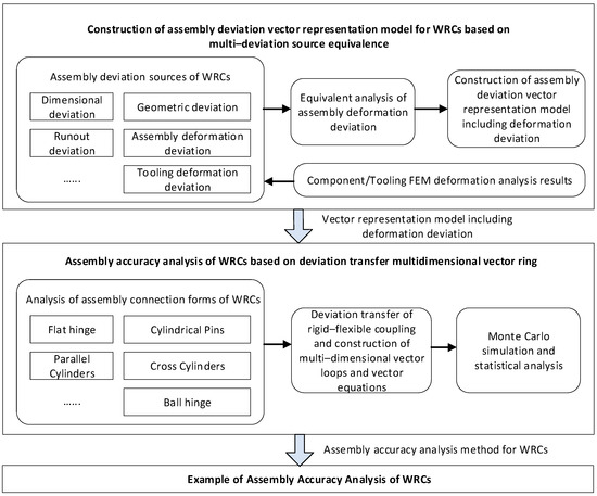
Figure 1.
Overall technical route of the project research.
Firstly, the assembly deviation sources of WRCs are analyzed, and the assembly deviation vector representation model is established based on the equivalence of multiple deviation sources. According to the characteristics of the assembly deviation direction and the diversity of transmission paths of WRCs, the assembly deviation sources are divided into dimensional deviation, geometric shape deviation, runout deviation, kinematic pair fit deviation, and assembly deformation deviation. For deviation sources that cannot be directly represented in the deviation model, such as assembly deformation deviation, a deviation equivalent model is established based on the principle of fit change to achieve expression in the deviation model, and then the WRC assembly multi-deviation source vector representation model is established.
Secondly, the assembly deviation transmission mechanism of WRCs is studied, and the assembly accuracy analysis model is constructed based on the multi-dimensional vector ring of deviation transmission. The accurate analysis of WRC assembly accuracy is achieved through the Monte Carlo method. The assembly connection forms and degrees of freedom of WRCs are analyzed, and the concepts of the deviation transmission reference path and deviation transmission path are defined. The deviation transmission paths under different assembly connection forms are studied. In the assembly matching part, the deviation transmission model describing the deviation transmission and accumulation mechanism is established based on vector representation, so as to establish a rigid–flexible coupled deviation transmission multi-dimensional vector loop model and vector equation, laying a model foundation for the analysis of WRC assembly accuracy. After establishing the deviation transmission multi-dimensional vector loop and vector equation, the Monte Carlo method is proposed to simulate and statistically analyze the assembly accuracy of WRCs.
4. Equivalent Analysis of Assembly Deformation Deviation Sources Based on Fit Changes
Assembly deformation refers to the elastic deformation of parts caused by loads such as the positioning clamping force and self-weight during assembly. This deformation not only affects part dimensions but also changes assembly positions. The following discusses the impact of assembly deformation on the part size and assembly position, and then studies the equivalent method of assembly deformation deviation.
- (1)
- Impact of assembly deformation on part size
The design dimensions of the part are expressed by the nominal value L and the tolerance T. The maximum and minimum allowable values of the length dimension of the part are L + T and L − T, respectively, as shown in Figure 2a. Under the action of assembly constraints and load F, the part undergoes axial deformation, where the deformation amount is δ (positive for tension and negative for compression). At this time, the maximum length dimension of the part is and the minimum is , as shown in Figure 2b.
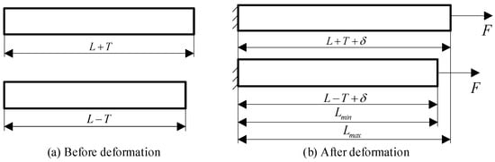
Figure 2.
The influence of assembly deformation on the part size.
Under the influence of assembly deformation, the size and deviation of the part in the deformation direction change to . Among them,
where and are the maximum and minimum size of the part in the deformation direction, respectively.
- (2)
- The influence of assembly deformation on the assembly position of parts
Assembly deformation affects the assembly position of parts, and a hinged motion mechanism is shown in Figure 3. When a rod with a nominal size of L rotates around the hinge at an angle of θ, if the assembly deformation is not considered, the part assembly is located at the position shown by the solid line in the figure. When taking the gravity G of the part into consideration, the part assembly is located at the position shown by the dotted line in the figure. It can be seen from the finite element method (FEM) that the axial deformation of the part under gravity is , and the radial deformation is . Among them, has an impact on the axial size L of the part, which is determined by . has an impact on the assembly position of the part, which is determined by the angle deviation of . The angle deviation can be obtained by Equation (3) based on the geometric relationship:
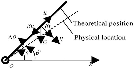
Figure 3.
The influence of assembly deformation on the assembly position of parts.
Then, the angle to determine the actual assembly position of the part is:
Among them, is the assembly position of the part without considering the assembly deformation; is the actual assembly position of the part after considering the assembly deformation; and is the assembly position deviation of the part caused by the assembly deformation, that is, the equivalent deviation.
Using the above equivalent method for assembly deformation deviation, the deformation is converted into part-size-related deviations. This allows the deviation source to be represented by a size vector, enabling a unified expression of multiple deviation sources in the deviation model. Based on this equivalence, the WRC assembly deviation vector representation model is then constructed.
5. Construction of Rigid–Flexible Coupling Multi-Dimensional Vector Ring Model Based on Assembly Constraints
5.1. Rigid Component Assembly Deviation Transfer Model and Vector Ring Equation Construction
5.1.1. The Principles of Deviation Transfer Path Construction Between Parts
During the assembly process, the deviation is transmitted between parts along specific paths through the assembly relationship. Therefore, the assembly connection types and degrees of freedom of components significantly influence deviation propagation. In the assembly of mechanical products, positioning is achieved through the positioning datum. Thus, when constructing deviation propagation paths, the first step is to establish the positioning datums for assembly components. According to the design datum, the assembly positioning datums of the parts are defined as the datum reference frame (DRF). The path formed by connecting the nominal dimension vector from the mating point to the DRF is defined as the datum flow chain (DFC). Following these definitions, Figure 4 illustrates the established DRFs and DFCs for a sample assembly. Figure 4a shows the assembly design model consisting of two components: a thin-shell part and a block part. At location A, the block is connected to the bottom of the thin-shell part through a face-to-face fit, and the connection is marked as JA, and the top of the thin-shell part is connected to the block part through a row of rivets, which is marked as JB at location B. HC is the fit clearance formed by the rivet connection, which is also an assembly functional requirement. The part DRFs are constructed in combination with the part design datum, and the datum paths DFC21 and DFC22 are established from the connection A between the two parts, and the datum paths DFC11 and DFC12 are established from the connection B, as shown in Figure 4b.
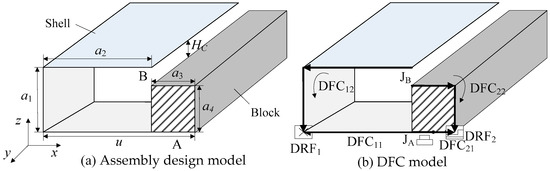
Figure 4.
Design models, DRFs, and DFCs.
After establishing the DFCs between two parts with the assembly constraint relationship, the path formed by the deviation transfer along the DFC is defined as the deviation transfer path. Through the analysis of the datum reference structure, datum flow chain and deviation transfer path construction process, the following four principles for creating assembly deviation transfer paths are summarized:
- (1)
- The deviation enters the interior of the part from the assembly connection. In the deviation transfer model shown in Figure 5, the deviation enters part i through the connection point J1 (part i − 1, part i) of the line–surface fit, and enters part i + 1 through the connection point J2 (part i, part i + 1) of the arc–arc fit.
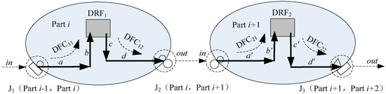 Figure 5. Deviation transformation model.
 - (2)
- Inside the part, the deviation reaches the DRF along the direction of the DFC. For example, inside part i as shown in Figure 5, the deviation reaches DRF1 along DFC11; inside part i + 1, the deviation reaches DRF2 along DFC21.
- (3)
- Inside the part, the deviation reaches another assembly connection along the direction of the second DFC. For example, inside part i as shown in Figure 5, the deviation reaches the assembly connection J2 (part i, part i + 1) along DFC12; inside part i + 1, the deviation reaches the assembly connection J3 (part i + 1, part i + 2) along DFC22.
- (4)
- The deviation exits the part from the assembly joint and enters the adjacent part.
In the deviation transfer model shown in Figure 5, the two parts are connected by the arc–arc. In part i, path a and b constitute the reference path DFC11, which means the path for the deviation to enter the interior of part i. Path c and d constitute the reference path DFC12, which is the path for the deviation to exit the interior of part i. After the deviation exits part i through DFC12, it is transferred along the reference path DFC21 of part i + 1, and then exits part i + 1 through DFC22. Under the constraints of the assembly connection relationship, the deviation is transferred in sequence along the paths DFC11, DFC12, DFC21, DFC22, etc., to form a deviation transfer path. Among them, a, b, c, d, a′, b′, c′, d′, etc., are called deviation transfer vectors. Since the controlled design dimensions and adjustable assembly dimensions are the occurrence parts of the deviation source in the assembly process, the establishment of the DFC must be along the direction of the design dimension or assembly dimension vector.
5.1.2. Deviation Transfer Vector Loop Construction in Assembly Process
According to the aforementioned principles, the deviation transfer path of multiple assembly parts in the assembly process is established according to the assembly connection form given by the design and the positioning method given by the process to form a deviation transfer vector loop. Based on the assembly function requirements and the characteristics of the deviation transfer path, the deviation transfer multi-dimensional vector loop is divided into a closed loop and an open loop.
Then, based on the assembly connection relationship, the method for establishing the deviation transfer vector loop of the assembly process is studied. As shown in Figure 6, assuming that both parts are rigid parts, according to the multi-dimensional vector loop modeling principles, the deviation is transferred along the path a, b, Hc, c, d, e′, e′′ to form a deviation transfer vector loop, Loop 1. Since the connection JB is achieved by multiple rivets, a series of spatial multi-dimensional vector loops can be constructed for each rivet connection point based on Loop 1 and combined with the rivet connection point spacing (fi, gi).
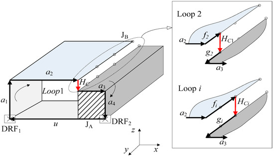
Figure 6.
Deviation transfer vector loop construction.
5.1.3. Deviation Transfer Vector Equation Construction
After establishing the deviation transfer multi-dimensional vector loop model, in order to realize the mathematical expression of the deviation transfer and accumulation, the deviation transfer vector equation is further established. Let represent the part size vector in the deviation transfer multi-dimensional vector loop, represent the geometric shape deviation vector in the multi-dimensional vector loop, represent the virtual connector size vector of the fit clearance in the multi-dimensional vector loop, and represent the assembly size vector in the multi-dimensional vector loop. Then, the assembly deviation transfer multi-dimensional vector equation can be expressed by a series of homogeneous matrix equations:
where [H] is the vector matrix of key feature function requirements.
5.2. Assembly Deviation Transfer Model of WRCs with Rigid–Flexible Coupling and Construction of Vector Loop Equation
The above-established assembly deviation transfer vector loop only contains the dimension vector, and it is assumed that all the parts contained in the assembly are rigid. However, in actual assembly processes, other deviation sources besides dimension deviation, such as part geometry deviation, assembly deformation and fit clearance, will affect the deviation transfer path and deviation accumulation results, consequently affecting the product’s ultimate assembly accuracy. In order to establish an assembly deviation transfer vector loop model containing multiple deviation sources, the following focuses on integrating the assembly deformation deviation vector, geometry deviation vector and fit clearance virtual connector deviation vector into the existing vector loop.
As shown in Figure 7a, the thin-shell part deforms under the action of the vertical assembly force Fi. The deformation θ can be obtained through the finite element calculation, and the thin-shell part in the assembly process model is replaced by the deformed finite element model. As can be seen from Figure 7, the deformation of the thin-shell part affects the dimension a2, forming a new dimension vector a2′. Since the assembly deformation of the thin-shell part is within the elastic deformation range of the material and the deformation angle θ is small, . At this time, the new dimension vector a2′ can be calculated by Equation (6):
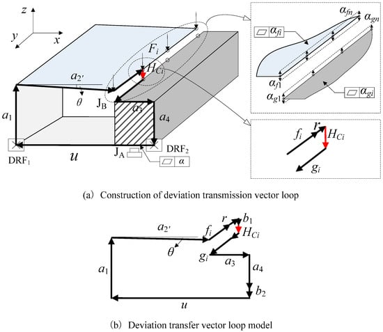
Figure 7.
Construction of the deviation transfer vector loop model of rigid–flexible coupling.
Taking the construction of the deviation transmission multi-dimensional vector loop Loop i of the rivet position (fi, gi) as an example, the deviation transmission multi-dimensional vector loop model under the action of assembly deformation is shown on the left side of Figure 7a.
At the connection point JB, the flatness of the surface to be connected is αfi, and the flatness of the target connection surface is αgi, as shown on the right side of Figure 7a. Assuming αfi < αgi, only the influence of αfi on the deviation transfer needs to be considered, and the flatness deviation vector is half of its tolerance zone, denoted as b1. Similarly, at the connection point JA, the flatness deviation vector is denoted as b2. In this example, the assembly of the thin-shell part and the block part is a clearance fit, so the fit clearance deviation is expressed by the size vector of the virtual connector, and the size vector of the fit clearance virtual connector is denoted as r. Finally, the deviation vectors b1, b2, and r are added to the deviation transfer multi-dimensional vector loop to establish a deviation transfer vector loop model containing multiple assembly deviation sources, as shown in Figure 7b.
After establishing the deviation transfer multi-dimensional vector loop model, in order to realize the mathematical expression of the deviation transfer and accumulation, the deviation transfer vector equation is further established. Let represent the part size vector in the deviation transfer multi-dimensional vector loop, represent the geometric shape deviation vector in the multi-dimensional vector loop, represent the virtual connector size vector of the fit clearance in the multi-dimensional vector loop, and represent the assembly size vector in the multi-dimensional vector loop. Then, the assembly deviation transfer multi-dimensional vector equation can be expressed by a series of homogeneous matrix equations:
where [H] is the vector matrix of key feature function requirements.
According to whether the multi-dimensional vector loop contains key characteristic requirements, the corresponding deviation transfer vector open loop and closed loop can be further established. The deviation transfer vector equation described in the above formula is decomposed in the closed-loop vector direction Λ and the open-loop vector direction Γ, as shown in the following formula:
where hc represents the deviation vector of the key control characteristic requirement in the closed-loop S direction; ho represents the deviation vector of the key control characteristic requirement in the open-loop Γ direction; Λ is the direction of the deviation transfer closed-loop vector; and Γ is the direction of the deviation transfer open-loop vector. So far, a multi-dimensional vector ring model of deviation transmission of rigid–flexible coupling assembly of WRCs has been established.
The established deviation transfer vector equation describes the nonlinear implicit functional relationship between the assembly key characteristic functional requirements and each deviation source. In order to obtain a linear and explicit deviation transfer function, the deviation transfer vector equation described by Equation (8) is linearized using Taylor expansion. The first-order Taylor expansion of the deviation transfer vector open-loop and closed-loop equations is:
where represents a small change in the functional requirement dimension, represents a dimension deviation, represents a small change in the geometric shape deviation, represents assembly deformation deviation, and represents a small change in the assembly dimension. At this time, the assembly deviation transfer scalar equation can be expressed as:
represents the partial derivative matrix of the deviation transfer equation for the part size, where represents the dimension deviation matrix of the assembly function requirements and means the dimension deviation matrix. represents the partial derivative matrix of the deviation transfer equation for the part geometry deviation and means the geometry deviation matrix. means the partial derivative matrix of the deviation transfer equation for assembly deformation, and indicates the assembly deformation deviation matrix. means the partial derivative matrix of the deviation transfer equation for the assembly size, and represents the assembly dimension deviation matrix.
The above formula is the linear equation for assembly deviation transmission. Based on this model, the Monte Carlo algorithm can be further used to analyze the assembly accuracy of WRCs.
6. Assembly Accuracy Analysis Algorithm Process Design Based on Monte Carlo Algorithm
The input data for the assembly accuracy analysis includes the product design tolerance, tooling design tolerance, assembly tolerance, flexible substructure FEA data, assembly process and other information. Among this information, the design tolerance, assembly tolerance and so on are tolerance zones, and the distribution states of individual random variables exhibit diversity. How to randomly extract a set of deviation values that meet the tolerance domain requirements from the tolerance band is the premise of assembly accuracy analysis, and the Monte Carlo method can effectively solve this problem.
The assembly accuracy simulation algorithm flow based on the Monte Carlo method is established and shown in Figure 8, which mainly includes sample quantity definition, tolerance information extraction and definition, random deviation generation, random sampling, assembly accuracy analysis value solution, simulation statistical parameter calculation, and simulation result output. The specific steps are as follows.
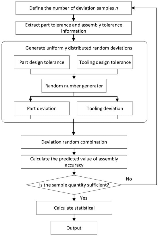
Figure 8.
Assembly accuracy analysis algorithm flow based on the Monte Carlo algorithm.
- Step 1: Define the deviation sample size n. A larger sample size increases the accuracy of assembly accuracy simulations. However, excessively large samples proportionally increase the computational time and cost. Since product assembly qualification rates do not require 100% perfection, a statistically representative Gaussian distribution can be approximated within limited computational time. Thus, this study sets the simulation frequency to 5000.
- Step 2: Extract and define tolerance information. Extract the part design tolerance in the design model and the assembly tolerance in the process model. Define the equivalent deviation information, tooling positioning tolerance and other information in the assembly accuracy information model as input information for the assembly accuracy simulation.
- Step 3: Generate random deviation. By using a random number generator, the deviation values in the tolerance domain are randomly extracted from the various tolerance information input in step 2 to generate random deviations.
- Step 4: Calculate the predicted value of assembly accuracy. Solve the assembly accuracy analysis function and calculate the assembly accuracy analysis value. If the sample quantity requirement is met, go to step 5; otherwise, go to step 1 to redefine the sample quantity n.
- Step 5: Statistical analysis of assembly accuracy prediction values. Perform statistical analysis on the calculated values of multiple samples, compare them with the predetermined assembly accuracy requirements (design requirements), and provide the predicted evaluation value and the average value and qualification rate of the calculation analysis function.
7. Case Study and Discussion
To validate the effectiveness of the proposed method, this section presents the assembly of a thin-walled frame (one of the WRCs) as an example and constructs the deviation transfer vector loop and vector equation of rigid–flexible coupling. The Monte Carlo method is applied to analyze the assembly accuracy, and the validity of the analysis results is explained.
The design model of the thin-walled frame assembly is shown in Figure 9a, including part A, part B, and part C. Part C is regarded as the basis, and parts A and B are assembled at the same time during assembly. In ideal assembly, there is no gap between the fitting surfaces of parts A and B. However, due to the deformation of thin-walled parts, manufacturing and process deviations, there is an assembly gap between the fitting surfaces of parts A and B in actual assembly, as shown by Gy in the Figure 9. The allowable tolerance of Gy is ±0.5 mm, which is the functional requirement for this assembly. Since Gy cannot be guaranteed through single point measurement, it is decomposed into multiple measurement points Gyi on the mating surface. By predicting the assembly accuracy of each measurement point Gyi on the mating surface, the assembly functional requirements of Gy can be ensured.
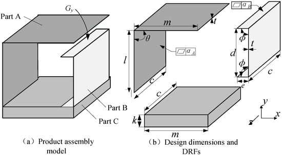
Figure 9.
Thin-walled frame assembly.
The design dimension parameters of the assembly are shown in Figure 9b, and the design dimensions and deviations are shown in Table 1.

Table 1.
Design dimensions and deviations of thin-walled frame assembly.
Firstly, based on the part design benchmark and assembly positioning benchmark, the DRFs (DRFA, DRFB, and DRFC) of the parts and assembly connection points Joints J (PB, PA), J (PC, PA), and J (PC, PB) are defined based on the assembly constraint relationships. The defined assembly DRFs and Joints are shown in Figure 10a. On this basis, the assembly connection form is analyzed, and according to the method and principles for constructing a deviation transfer multi-dimensional vector loop proposed in Section 5.2, a deviation transfer multi-dimensional vector loop for the thin-walled frame assembly is established, as shown in Figure 10b.
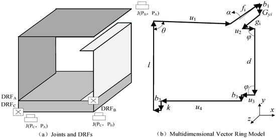
Figure 10.
Multi-dimensional vector loop model for deviation transmission in thin-walled frame assembly.
In this multi-dimensional vector loop model of assembly deviation transmission for the thin-walled frame, Gyi is the assembly clearance deviation vector of the i-th measurement point on the mating surface. φl, d, k are angle or size vectors, while θ and α are the angle deviation introduced by the deformation of the part. bi is the geometric deviation vector, and u1, u2, u3, u4 are assembly dimension vectors. fi and gi are the measurement point position size vectors required for functional requirements.
Secondly, based on the multi-dimensional vector loop of assembly deviation transmission, the vector equation is established according to Formula (5). Since there is only vector open loop and no vector closed loop in this example, the deviation transfer vector equation is established in the direction of vector open loop, as shown in Equation (11).
Then, the above equation is linearized according to Equation (9) and the parameters are solved, as shown in Equation (12):
Since this example only has open-loop vector equations, there are no parameters A, B, R, and U. According to Formula (10), the accuracy analysis function for assembly clearance is defined as:
Finally, assembly accuracy simulation is conducted based on the Monte Carlo method, with ±0.5 mm specified as the upper and lower limits allowed for assembly clearance. The simulation times are set to n = 5000, and the obtained simulation results are shown in Figure 11a.
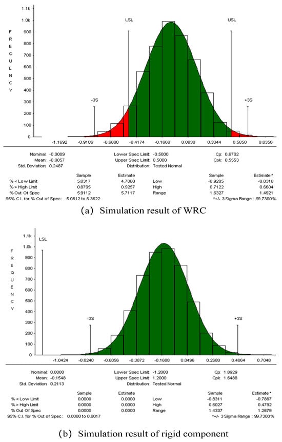
Figure 11.
Accuracy simulation results of assembly gap Gyi in a thin-walled frame.
According to the simulation results, the probability of the Gyi deviation exceeding ± 0.5 mm is 5.91%, and the predicted average assembly accuracy of the gap is 0.248 mm. To demonstrate the effectiveness of the assembly deviation transfer model and accuracy analysis for WRCs, the accuracy of the assembly gap Gyi of the thin-walled frame is simulated and predicted using the rigid component deviation transfer model and accuracy analysis method. The simulation results show no deviation, and the predicted average assembly accuracy of the gap is 0.211 mm. A comparison of the results obtained from the two accuracy analysis methods is shown in Table 2.
Table 2.
Comparison of different assembly accuracy analysis methods with measured values.
When the rigid component accuracy analysis method is applied, the influence of assembly deformation deviation is not considered, and the obtained assembly qualification rate is higher. From the simulation results, the qualification rate is 100%, which meets the design requirements. However, the assembly accuracy and assembly qualification rate obtained by the WRC assembly accuracy analysis method proposed in this paper are relatively low (94.09%). The probability that the assembly gap between the mating surfaces of parts A and B is within the design range is 94.09%, which cannot meet the assembly accuracy requirements under the 3σ quality criterion, It is necessary to further optimize the assembly deviations and the assembly process.
This indicates that accounting for weak rigidity issues enables comprehensive coverage of the assembly deviation sources, thereby ensuring safer assembly processes and more reliable assembly accuracy analysis results.
8. Conclusions
To address the impact of assembly deformation on the accuracy of assembly accuracy analysis for WRCs, this study proposes a novel assembly accuracy analysis method. Through equivalent analysis of the deformation deviation, a unified deviation vector representation model that conforms to the actual WRC assembly is established. Based on the multi-dimensional vector loop, the assembly deviation transmission mechanism is investigated, leading to the development of a rigid–flexible coupled deviation propagation model that reveals the influence patterns of the mating configurations and datum references on the assembly accuracy in WRCs. Furthermore, a computational method for accumulated deviation propagation in rigid–flexible coupled WRCs is developed, with case studies validating the reliability of the proposed approach. This method provides a theoretical basis and implementation method for assembly accuracy simulation of WRCs, and it can improve the reliability of assembly accuracy analysis results for WRCs.
Author Contributions
Conceptualization, D.Z.; methodology, D.Z.; software, X.Z.; validation, X.Z. and Z.Y.; writing—original draft preparation, D.Z.; writing—review and editing, G.W. All authors have read and agreed to the published version of the manuscript.
Funding
This research was funded by the Natural Science Basic Research Project of Shaanxi Province, China, grant numbers 2025JC-YBMS-584 and 2025JC-YBMS-565.
Data Availability Statement
The original contributions presented in this study are included in the article. Further inquiries can be directed to the corresponding author.
Conflicts of Interest
The authors declare no conflict of interest.
Correction Statement
This article has been republished with a minor correction to the Data Availability Statement. This change does not affect the scientific content of the article.
References
- Maltauro, M.; Passarotto, G.; Concheri, G.; Meneghello, R. Bridging the gap between design and manufacturing specifications for non-rigid parts using the influence coefficient method. Int. J. Adv. Manuf. Technol. 2023, 127, 579–597. [Google Scholar] [CrossRef]
- Atik, H.; Chahbouni, M.; Amegouz, D.; Boutahari, S. Optimization tolerancing of surface in flexible parts and assembly: Influence Coefficient Method with shape defects. Int. J. Eng. Technol. 2018, 7, 90. [Google Scholar] [CrossRef]
- Polini, W.; Corrado, A. Methods of influence coefficients to evaluate stress and deviation distribution of flexible assemblies—A review. Int. J. Adv. Manuf. Technol. 2020, 107, 2901–2915. [Google Scholar] [CrossRef]
- Hillyard, R.C.; Braid, I.C. Characterizing non-ideal shapes in terms of dimensions and tolerances. Acm Siggraph Comput. Graph. 1978, 12, 234–238. [Google Scholar] [CrossRef]
- Zhang, B.C. Geometric Modeling of Dimensioning and Tolerancing. Ph.D. Thesis, Arizona State University, Tempe, AZ, USA, 1992. [Google Scholar]
- Shen, T.H.; Lu, C. An assembly accuracy analysis approach of mechanical assembly involving parallel and serial connections considering form defects and local surface deformations. Precis. Eng. 2024, 88, 44–64. [Google Scholar] [CrossRef]
- Zhao, B.; Wang, Y.; Sun, Q.; Zhang, Y.; Liang, X.; Liu, X. Monomer model: An integrated characterization method of geometrical deviations for assembly accuracy analysis. Assem. Autom. 2021, 41, 514–523. [Google Scholar] [CrossRef]
- Cui, L.; Sun, M.; Cao, Y.; Zhao, Q.J.; Zeng, W.-H.; Guo, S.-R. A novel tolerance geometric method based on machine learning. J. Intell. Manuf. 2021, 32, 799–821. [Google Scholar] [CrossRef]
- Laifa, M.; Sai, W.B.; Hbaieb, M. Evaluation of machining process by integrating 3D manufacturing dispersions, functional constraints, and the concept of small displacement torsors. Int. J. Adv. Manuf. Technol. 2014, 71, 1327–1336. [Google Scholar] [CrossRef]
- Jin, S.; Chen, H.; Li, Z.; Lai, X. A small displacement torsor model for 3D tolerance analysis of conical structures. Proc. Inst. Mech. Eng. Part C J. Mech. Eng. Sci. 2015, 229, 2514–2523. [Google Scholar] [CrossRef]
- Wu, Y.G. Tolerance mathematical model based on the variation of control points of geometric elemen. J. Mech. Eng. 2013, 5, 138. [Google Scholar] [CrossRef]
- Guo, F.; Bao, Q.; Liu, J.; Sha, X. Assembly quality control technologies in forced clam and compensation processes for large and integrated aeronautical composite structures. Machines 2025, 13, 159. [Google Scholar] [CrossRef]
- Cao, Y.L.; Srinivasan, V. Special Issue: Geometric tolerancing. J. Comput. Inf. Sci. Eng. 2015, 15, 44–57. [Google Scholar] [CrossRef]
- Anwer, N.; Schleich, B.; Mathieu, L.; Wartzack, S. From solid modelling to skin model shapes: Shifting paradigms in computer-aided tolerancing. CIRP Ann.-Manuf. Technol. 2014, 63, 137–140. [Google Scholar] [CrossRef]
- ASME. Dimensioning and Tolerancing Principles. In ANSI Standard Y14.5M; ASME: New York, NY, USA, 1994. [Google Scholar]
- Johnson, R.H. Dimensioning and Tolerancing Final Report; Report R-84GM-02.2; Computer Aided Manufacturing International: Arlington, TX, USA, 1985. [Google Scholar]
- Roy, U.; Liu, C.R. Feature-based representational scheme of a solid modeler for providing dimensioning and tolerancing information. Robot. Comput.-Integr. Manuf. 1988, 4, 335–345. [Google Scholar] [CrossRef]
- Mujezinovic, A.; Davidson, J.K.; Shah, J.J. A new mathematical model for geometric tolerances as applied to polygonal faces. Int. J. Mech. Des. 2004, 126, 504–518. [Google Scholar] [CrossRef]
- Desrochers, A.; Desrochers, A. A CAD/CAM representation model applied to tolerance transfer methods. Int. J. Mech. Des. 2003, 125, 22–31. [Google Scholar] [CrossRef]
- Liu, Y.; Gao, S.; Wu, Z.; Yang, J. Feature-based hierarchical tolerance information representation model and its implementation. Int. J. Mech. Eng. 2003, 39, 1–7. [Google Scholar]
- Glancy, C.G.; Chase, K.W. A Second-Order method for assembly tolerance analysis; American Society of Mechanical Engineers: New York, NY, USA, 1999; pp. 977–984. [Google Scholar]
- Chase, K.W.; Gao, J.; Magleby, S.P.; Spencer, P.M. General 2-D tolerance analysis of mechanical assemblies with small kinematic adjustments. J. Des. Manuf. 1995, 5, 263–274. [Google Scholar]
- Tang, W.; Li, Y.; Yan, T.; Zhang, M. Assembly accuracy analysis method based on multi-stage linearized contact. Eng. Rep. 2025, 7, e13118. [Google Scholar] [CrossRef]
- Liu, S.G.; Wang, P.; Li, Z.G. Non-normal statistical tolerance analysis using analytical convolution method. Int. J. Adv. Manuf. Technol. 2011, 7, 127–130. [Google Scholar] [CrossRef]
- Marler, J.D. Nonlinear tolerance analysis using the direct linearization method. Ph.D. Thesis, Brigham Young University Department of Mechanical Engineering, Provo, UT, USA, 1988. [Google Scholar]
- Tsai, J.C.; Kuo, C.H. A novel statistical tolerance analysis method for assembled parts. Int. J. Prod. Res. 2012, 50, 3498–3513. [Google Scholar] [CrossRef]
- Cao, Y. Dynamic prediction and compensation of aerocraft assembly variation based on state space model. Assem. Autom. 2015, 35, 183–189. [Google Scholar] [CrossRef]
- Hu, W.; Liu, J.H.; Jiang, K.; Guo, C.Y. Assembly precision prediction method for spacecraft based on 3D model. Comput. Integr. Manuf. Syst. 2013, 19, 990–999. [Google Scholar]
- Polini, W.; Corrado, A. Geometric tolerance analysis through Jacobian model for rigid assemblies with translational deviations. Assem. Autom. 2016, 36, 72–79. [Google Scholar]
- Guo, F.; Hou, Y.; Xiao, Q.; Zhang, X.; Xiao, S.; Wang, Z. Reliability improvement on assembly accuracy with maximum out-of-tolerance probability analysis and prior precise repair optimization. Adv. Eng. Inform. 2023, 55, 101866. [Google Scholar]
- Yang, J.; Wang, J.; Wu, Z.; Anwer, N. Statistical tolerancing based on variation of point-set. Procedia Cirp 2013, 10, 9–16. [Google Scholar] [CrossRef]
- Liu, S.C.; Hu, S.J. Variation Simulation for Deformable Sheet metal assemblies using finite element methods. J. Manuf. Sci. Eng. 1997, 119, 368–374. [Google Scholar] [CrossRef]
- Spathopoulos, S.C.; Stavroulakis, G.E. Springback prediction in sheet metal forming based on finite element analysis and artificial neural Network Approach. Appl. Mech. 2020, 1, 97–110. [Google Scholar] [CrossRef]
- Liu, Y.; Zhao, Y.; Lin, Q.; Pan, W.; Wang, W.; Ge, E. Deviation GAN: A generative end-to-end approach for the deviation prediction of sheet metal assembly. Mech. Syst. Signal Process. 2023, 204, 110822. [Google Scholar] [CrossRef]
- Shi, S.; Liu, J.; Gong, H.; Shao, N.; Anwer, N. Assembly accuracy analysis and phase optimization of aero-engine multistage rotors considering surface morphology and non-uniform contact deformation. Precis. Eng. 2024, 88, 595–610. [Google Scholar] [CrossRef]
- Dupac, M.; Beale, D.G. Dynamic analysis of a flexible linkage mechanism with cracks and clearance. Mech. Mach. Theory. 2010, 45, 1909–1923. [Google Scholar] [CrossRef]
- Yan, J.; Ding, H.; Liang, H. Application of Digital Twin technology in high-precision assembly: Structural accuracy analysis and rework optimization for large-scale equipment. Int. J. Adv. Manuf. Technol. 2025, 138, 1229–1250. [Google Scholar] [CrossRef]
- Imani, B.M.; Pour, M. Tolerance analysis of flexible kinematic mechanism using DLM method. Mech. Mach. Theory. 2009, 44, 445–456. [Google Scholar] [CrossRef]
- Schleich, B.; Anwer, N.; Mathieu, L.; Wartzack, S. Skin Model Shapes: A new paradigm shift for geometric variations modelling in mechanical engineering. Comput. Aided Des. 2014, 50, 1–15. [Google Scholar] [CrossRef]
- Franciosa, P.; Gerbino, S.; Patalano, S. Simulation of variational compliant assemblies with shape errors based on morphing mesh approach. Int. J. Adv. Manuf. Technol. 2011, 53, 47–61. [Google Scholar] [CrossRef]
Disclaimer/Publisher’s Note: The statements, opinions and data contained in all publications are solely those of the individual author(s) and contributor(s) and not of MDPI and/or the editor(s). MDPI and/or the editor(s) disclaim responsibility for any injury to people or property resulting from any ideas, methods, instructions or products referred to in the content. |
© 2025 by the authors. Licensee MDPI, Basel, Switzerland. This article is an open access article distributed under the terms and conditions of the Creative Commons Attribution (CC BY) license (https://creativecommons.org/licenses/by/4.0/).