Abstract
Omnidirectional mobile robots have gained extensive application across diverse fields due to their exceptional maneuverability and adaptability in confined spaces. However, structural and systemic uncertainties significantly compromise motion accuracy. To enhance motion control precision, this paper proposes a sliding mode control (SMC) method integrated with a radial basis function (RBF) neural network. The approach aggregates model uncertainties, nonlinear dynamics, and unknown disturbances into a composite disturbance term. An RBF neural network is employed to approximate this disturbance, with compensation embedded within the SMC framework. An online adaptive law for neural network optimization is derived using the Lyapunov stability theorem, thereby improving the disturbance rejection capability. Comparative simulations and experiments validate the proposed method against modern control strategies. Results demonstrate superior tracking performance and robustness, significantly enhancing trajectory tracking accuracy for the MY3 wheeled omnidirectional mobile robot.
1. Introduction
Omnidirectional mobile robots can achieve in-place steering and flexible movement in confined spaces, significantly improving space utilization efficiency. This capability has important applications in environments with high demands for space management, such as urban settings, factory workshops, and warehouse systems. The high flexibility and maneuverability of omnidirectional mobile robots make them suitable for various application scenarios, including but not limited to agriculture [1], manufacturing [2], and healthcare [3]. During the motion of omnidirectional mobile robots, they face complex factors such as friction, load variations, environmental condition changes, and non-Gaussian noise, making it challenging to obtain an accurate mathematical model. Inaccuracies in internal modeling and external environmental disturbances can affect the robots’ motion accuracy. To address this issue, researchers have explored various control strategies, including the use of disturbance observers to estimate and compensate for disturbances within the system, thereby reducing their impact. Observers such as the generalized proportional integral observer [4], the extended state observer [5,6], the sliding mode disturbance observer [7], and improved generalized proportional integral observer [8] have been designed to tackle this problem. These observers can effectively estimate and compensate for disturbances, enhancing system robustness. However, they present challenges such as complex parameter tuning and strong dependence on the model. Active disturbance rejection control [9] is a control strategy that combines state observers and feedback control, enabling real-time estimation of and compensation for external disturbances. It effectively addresses external disturbances and system uncertainties but involves complex parameter adjustment. Optimal control [10] designs controllers by optimizing performance indices, such as energy consumption [11,12] and error, with common methods including the linear quadratic regulator [13] and dynamic programming. Through optimal control, performance indices can be systematically optimized; however, unforeseen disturbances and variations in practical applications can still affect control efficacy. Model predictive control [14,15,16] predicts the future behavior of the system and takes appropriate measures in advance, solving optimization problems within a finite time horizon at each control instant. It considers potential future disturbances and uncertainties during optimization, thus providing robustness against model uncertainties and external disturbances. However, model predictive control demands highly computational resources, especially for large-scale systems or real-time control applications, and its performance is highly dependent on the accuracy of the system model.
Sliding mode control [17] is a nonlinear robust control method particularly suited for handling system uncertainties and external disturbances. Its core principle involves designing a sliding surface, along which the system slides to achieve stable control. To reduce dependence on uncertain parameters, a robust adaptive terminal sliding mode control method [18] and an adaptive integral terminal sliding mode control method [19] have been successfully applied to omnidirectional mobile robots. Both methods exhibit strong robust tracking performance and finite-time error convergence. However, the frequent switching of control signals near the sliding surface induces high-frequency chattering, which affects system performance and practical application. To address this issue, a super-twisting algorithm [20] has been proposed. The super-twisting algorithm is a variant of second-order sliding mode control designed to mitigate chattering problems in traditional sliding mode control while enhancing system robustness and control performance. Nonetheless, the super-twisting algorithm faces challenges with complex parameter tuning. Another approach involves using boundary layer techniques, which introduce a small range of continuous control regions near the sliding surface to smooth the sliding mode control input.
In recent years, research has increasingly focused on intelligent control methods. Compared to traditional control methods, intelligent control is more suitable for controlling uncertain systems. Among these, fuzzy control [21,22,23,24] excels in handling uncertainties and imprecise information, does not require precise mathematical models, is easy to understand and implement, and offers strong robustness, making it suitable for nonlinear systems and complex environments. However, fuzzy control faces challenges such as complex rule base design and dependence on expert knowledge. Neural network control [25,26,27], on the other hand, possesses self-learning and adaptive capabilities, can handle high-dimensional data and complex systems, and offers nonlinear approximation and good generalization abilities, making it suitable for scenarios requiring real-time and high-precision control. A model predictive control method based on convolutional neural networks [28] has been applied to omnidirectional mobile robots. Convolutional neural networks are suitable for handling high-dimensional data (such as images and videos) and complex pattern recognition tasks. However, training convolutional neural networks requires large amounts of data, and for control tasks that need to handle temporal relationships and dynamic changes, such as robot path planning and motion control, convolutional neural networks are less suitable compared to other networks. Researchers have combined fuzzy control and neural network control, proposing a control method based on interval type-2 fuzzy neural networks [29,30]. This approach combines the advantages of interval type-2 fuzzy logic systems and neural networks, offering significant advantages in handling complex and uncertain systems. However, it has high complexity and implementation difficulty, requires large amounts of training data, involves substantial computational effort, has complex parameter tuning, and poses challenges in theoretical analysis. To meet real-time control requirements, a control method based on radial basis function neural networks (RBFNNs) [31,32] has been applied to omnidirectional mobile robots. RBFNNs can approximate arbitrarily complex nonlinear functions. Compared to other neural networks, RBFNNs have a simple structure, are easy to implement and understand, and are suitable for engineering applications. Due to the use of fixed radial basis functions in the hidden layer, RBFNNs have relatively fast training speeds, typically only requiring adjustment of the output layer weights. The output of hidden layer nodes depends only on the distance between input vectors and center vectors, offering good local generalization capabilities. RBFNNs can effectively handle local features and facilitate online learning by continuously adjusting the parameters of hidden layer nodes and the weights of the output layer, thus achieving real-time control. A set point optimization method for multilayer control systems employs terminal sliding mode control to ensure subsystem stability and incorporates an outer-layer learning mechanism to compensate for uncertainties [33]. Additionally, a neural adaptive command-filtered backstepping control is presented, which uses an RBF neural observer to estimate states/uncertainties, addresses the “complexity explosion” problem via command filtering with error compensation, and handles input saturation with smooth hyperbolic functions [34]. These approaches enhance control performance for complex industrial processes and enable high-precision trajectory tracking in flexible-joint manipulators under limited state feedback.
The remainder of this paper is organized as follows: Section 2 introduces the robot’s hardware setup and mathematical model. Section 3 presents the sliding mode control method for the MY3 omnidirectional mobile robot based on RBF neural networks. Section 4 provides the analysis of simulation results. Section 5 describes the experimental validation. Finally, Section 6 summarizes the main conclusions of this study.
The main contributions of this paper are as follows:
- (1)
- A sliding mode controller integrated with a radial basis function (RBF) neural network is developed, wherein a hyperbolic tangent function-based sliding surface is designed to effectively attenuate the high-frequency chattering phenomenon inherent in traditional sliding mode control;
- (2)
- To address modeling inaccuracies and unknown external disturbances in the MY3 omnidirectional mobile robot system [35], an online learning RBF neural network is engineered to achieve real-time compensation for aggregated system disturbances;
- (3)
- Comprehensive simulations and physical experiments conducted on the MY3 omnidirectional mobile robotic platform validate the robustness and engineering implementability of the proposed methodology in complex trajectory tracking tasks.
2. Structure and System Model
2.1. Structure of MY3-OMR
As shown in Figure 1a, the MY3 omnidirectional mobile robot (MY3-OMR) consists of four MY3 wheel modules, an upper frame, a lower frame, and a suspension system. The four MY3 wheel modules are uniformly fixed to the lower frame. The lower frame is divided into left and right sections, with the left side fixedly connected to the upper frame through profile sections, and the right side connected to the upper frame via the suspension system. The MY3 wheel module utilizes synchronous belt drive. Figure 1b illustrates the omnidirectional movement principle of the MY3 wheel. The usage of MY3 wheels is similar to that of orthogonal wheels; a single double-spherical-cap differential wheel can only achieve partial omnidirectional movement. However, when two double-spherical-cap differential wheels are combined, they form a mechanism capable of achieving full omnidirectional movement within a plane.

Figure 1.
Mobile robot and movement principle: (a) MY3 wheeled omnidirectional mobile robot; (b) movement principle.
2.2. System Modeling
As shown in Figure 2, the mathematical model of the MY3-OMR is established, assuming that the robot’s center of mass coincides with its geometric center. The parameters in the model are defined as listed in Table 1.
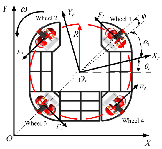
Figure 2.
MY3-OMR model diagram.

Table 1.
Definition of parameters.
The kinematic model of the MY3-OMR is established using the velocity equation method, where
represents the pose of the omnidirectional mobile robot in the global coordinate system.
represents the velocity vector of the omnidirectional mobile robot in the global coordinate system.
The kinematic equations of the MY3-OMR are as follows:
The direct kinematic model for it is as follows:
Therefore, its inverse kinematic model is as follows:
where represents the velocity Jacobian matrix of the mobile robot.
From this, the mapping relationship between the system inputs and outputs is derived, obtaining the corresponding relationship between the rotational angular velocities of the MY3 wheels and the velocity of the omnidirectional mobile robot in the world coordinate system.
Using the Newton–Euler method, the dynamic model of the MY3-OMR is established. The dynamic model of the MY3-OMR is as follows:
where
: The mass of the omnidirectional mobile robot.
: Moments of inertia.
are the Coulomb friction forces.
are the viscous friction forces.
are the Coulomb torque and viscous torque, respectively.
are the traction forces in the x-direction, y-direction, and the traction torque in the world coordinate system, respectively.
The mechanical relationship between the driving force Fi (i = 1,2,3,4) of each wheel assembly and the motor torque Ti (i = 1,2,3,4) is given using the following:
By performing force analysis on the omnidirectional mobile robot, we can deduce the following using the principle of vector composition:
From Equations (4)–(6), we obtain the dynamic model of the MY3 omnidirectional mobile robot as follows:
where
is the inertia matrix.
is the viscous friction coefficient matrix.
is the Coulomb friction coefficient matrix.
represents the uncertain disturbances in the system.
represents the matrix of motor input torques for each wheel assembly.
is the force Jacobian matrix of the omnidirectional mobile robot.
Typically, for the convenience of designing traditional model-based controllers, , , and are assumed to be zero. However, in practical motion, MY3 omnidirectional mobile robots are often affected by unmodeled nonlinear disturbances and external interferences from the operational environment, which can significantly impact system performance. Because these parameters are difficult or impossible to measure in most cases, this paper proposes a control method that does not rely on these model parameters.
3. Design of Control System
3.1. Uncertainty in Model Parameters
Handling the uncertainty in model parameters effectively is crucial for ensuring the robustness of system control. Parameters in dynamic systems such as the viscosity friction coefficient matrix C and the Coulomb friction coefficient matrix G may vary slightly during the robot’s motion. Although the precise values of these system parameters are unknown in practice and are difficult to measure accurately in real time using sensors, it is reasonable to assume their boundary conditions as follows:
where and are the lower bounds of the viscosity friction coefficient matrix and Coulomb friction coefficient matrix, respectively, and and are the upper bounds of the viscosity friction coefficient matrix and Coulomb friction coefficient matrix, respectively.
3.2. Robust Sliding Mode Control
From the dynamic model equations in Section 2, specifically Equation (7), we obtain the following:
When defining the state variables of the system and , the state-space representation of the system is given using the following:
Abbreviated form of Equation (10):
The following can be obtained:
represents the combined effect of viscous friction and Coulomb friction on the robot. represents the control input of the system, and represents the external disturbance term, which satisfies . In practical engineerng, the model uncertainty is denoted as . Based on the boundary conditions discussed in the previous section, the expression for the upper bound of , denoted as , is obtained as follows:
When defining the desired pose as , the tracking error is as follows:
The sliding mode function is defined as follows:
where , then the following holds:
The control input equation is as follows:
In Equation (16), represents the hyperbolic tangent function, which is defined as follows:
Defining the Lyapunov function as follows:
By substituting Equation (16) into Equation (15), we obtain the following:
If we choose , we obtain the following:
Thus, the control law for robust sliding mode control is derived, and its stability is proven using the Lyapunov function. Additionally, boundary layer techniques are applied, and a hyperbolic tangent function is used to replace the traditional switching function. The hyperbolic tangent function can smooth the control signal, avoiding the chattering phenomenon caused by rapid switching, thereby reducing high-frequency oscillations in the system. However, in practical applications, it is often difficult to obtain the complete dynamic information of an uncertain system. Further research is needed on sliding mode control algorithms to address trajectory tracking control problems without relying on information about system uncertainties and disturbances.
3.3. RBF Neural Network Sliding Mode Control
Since f is unknown, we can use an RBF neural network to approximate the uncertain term f and compensate it into the sliding mode control. As shown in Figure 3, Figure 3a is the distribution of Gaussian basis functions in the hidden layer, and Figure 3b is the structure diagram of the radial basis function neural network. The network algorithm is as follows:
where x is the input to the network; i is the number of inputs to the network; j is the index of the j-th node in the hidden layer of the network; is the coordinate vector of the center point of the j-th Gaussian basis function in the hidden layer; is the output of the Gaussian function; are the desired weights of the network; is the width of the Gaussian basis function of the j-th neuron in the hidden layer; is the approximation error of the network; and .
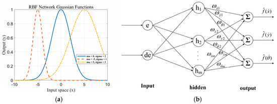
Figure 3.
RBF neural network: (a) Distribution of Gaussian basis functions in the hidden layer; (b) structural diagram of radial basis function neural network.
If the network input is , then the output of the RBF network is as follows:
where is the Gaussian function of the RBF neural network.
Therefore, the control input Equation (16) can be written as follows:
By substituting the control law Equation (18) into Equation (15), we obtain the following:
where
In Equation (20), represents the weight error.
Based on the above analysis, the complete form of the RBF neural network sliding mode control law can be obtained. This control law is composed of the neural network adaptive compensation term, sliding surface switching term, and desired trajectory feedforward term. The neural network performs real-time approximation of the system’s uncertain terms and continuously updates the network weights through the adaptive law to gradually reduce the approximation error. The sliding mode term enhances the system’s disturbance rejection capability by introducing a smooth switching function while effectively suppressing sliding mode chattering. The overall control law not only balances the adaptive compensation for the system’s unknown dynamics, but also possesses excellent robustness and dynamic performance. The system control block diagram is shown in Figure 4.
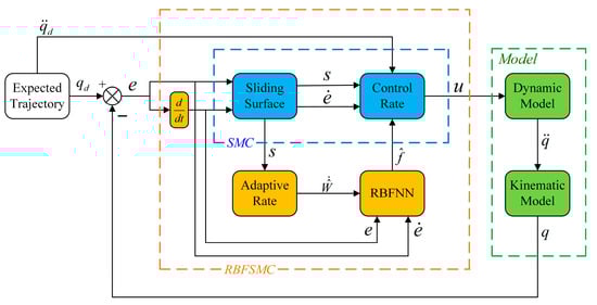
Figure 4.
System control block diagram.
Defining the Lyapunov function as follows:
where .
Taking the derivative of the Lyapunov function , we obtain the following:
Designing the adaptive law as follows:
Therefore,
Since the approximation error can be sufficiently small, and choosing , we obtain .
There exists , such that the following holds:
Due to , and are bounded. When and , according to the Lyapunov direct method, the closed-loop system is asymptotically stable. At , , hence and .
4. Simulation Experiment
The proposed control system was subjected to simulation to verify the effectiveness of the designed control method. To ensure an objective comparison, the same reaching law was set for the sliding mode control, the reduced-order extended state observer sliding mode control (ROESOSMC), and the RBF neural network sliding mode control in the simulations. The core concept of the reduced-order sliding mode control strategy involves employing a reduced-order extended state observer to estimate partial state variables and the total disturbance in real time. This estimation is then integrated with a sliding mode controller to formulate the control law, thereby enhancing system robustness and disturbance rejection capability. This controller is particularly suitable for systems where partial state measurements are available and disturbances are unknown but bounded [5,6]. Additionally, to evaluate the stability of the controllers, external disturbances were introduced, and the following commonly used performance indicators were selected to intuitively assess tracking performance:
where IAE stands for Integral of Absolute Error and RMSE stands for Root Mean Square Error. The IAE calculates the integral of the absolute value of the error over the entire time range, treating the magnitude of the error equally without amplifying larger errors. The RMSE calculates the square root of the mean of the squares of the error, amplifying larger errors due to squaring, thus highlighting the impact of larger errors more effectively. Therefore, selecting these two metrics can comprehensively evaluate the control performance when validating the control method.
To more accurately capture the uncertainties present in real-world systems, the disturbance term was modeled within the simulation. Specifically, it was configured as a random variable uniformly distributed over the interval [−0.1, 0.1], accounting for external disturbances, modeling errors, or sensor noise. During each control cycle, this disturbance is randomly updated and persistently applied to the system input. This approach is employed to rigorously evaluate the controller’s robustness and tracking performance under non-ideal conditions.
4.1. Simulation Analysis Under Varied Road Surface Conditions
In this simulation section, a comparison is made between sliding mode control, the proposed RBF neural network sliding mode control method, and ROESOSMC in terms of their path-tracking performance under varying road surface conditions. The aim is to verify the robustness of the proposed control method in coping with changes in the road surface environment. The model parameters are shown in Table 2.
Table 2.
Model parameters.
Assuming that the vehicle traverses three different road surfaces during the time intervals 0 to 10 s, 10 to 20 s, and 20 to 30 s, the corresponding Coulomb friction coefficients are as follows:
The formula for Coulomb torque is as follows:
where is the Coulomb friction coefficient, is the applied normal force, and is the radius of action.
Therefore, the Coulomb torque under different road surface conditions is as follows:
Set the simulation time to 30 s, simulate tracking a circular trajectory, and provide the desired trajectory of the robot:
Let be the radius of the circle, and the angular velocity . The initial position is as follows:
As shown in Figure 5, three controllers effectively track the predefined trajectory, with the RBF-SMC controller demonstrating superior tracking accuracy. To objectively evaluate the tracking performance, the relevant performance metrics are calculated based on Equations (22) and (23), with the results presented in Table 3.
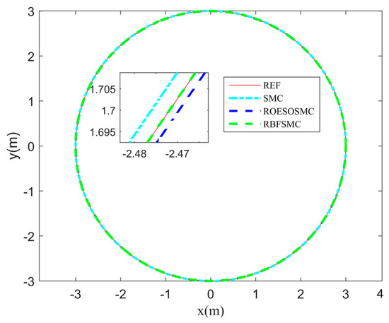
Figure 5.
Circular trajectory tracking with varying road surface conditions.
Table 3.
IAE and RMSE of circular trajectory under varying road surface conditions.
The tracking performance under different road surface conditions is illustrated in Figure 6, Figure 7 and Figure 8. Figure 6 depicts the trajectory and velocity tracking in the x-direction and Figure 7 shows the trajectory and velocity tracking in the y-direction. Figure 8 presents the angle and angular velocity tracking in the -direction. It can be observed that when the road surface condition transitions from a dry asphalt surface to an icy and snowy surface at t = 10 s, and further transitions to a wet asphalt surface at t = 20 s, the RBF-SMC method exhibits strong robustness to changes in Coulomb friction coefficients and Coulomb torque. This demonstrates its capability to effectively handle dynamic changes under complex road surface conditions.
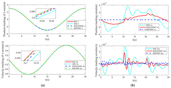
Figure 6.
Tracking performance in the x-direction under varied road surface conditions: (a) Trajectory tracking performance in the x-direction; (b) trajectory tracking error in the x-direction.
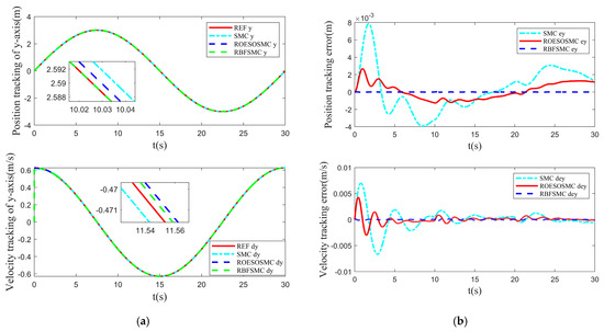
Figure 7.
Tracking performance in the y-direction under varied road surface conditions: (a) Trajectory tracking performance in the y-direction; (b) trajectory tracking error in the y-direction.
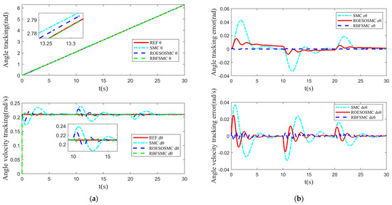
Figure 8.
Heading angle θ tracking performance under varied road surface conditions: (a) Heading angle θ tracking performance; (b) heading angle θ tracking error.
Figure 9 illustrates the variations in the control input signals under the three control strategies. The sliding mode control based on the radial basis function neural network (RBFNN-SMC) exhibits superior smoothness in the control input compared to the sliding mode control based on the reduced-order extended state observer (ROESO-SMC), which itself demonstrates better smoothness than traditional sliding mode control (SMC). The RBFNN-SMC approach employs the neural network to perform online approximation and compensation for system uncertainties and external disturbances. This reduces reliance on the sliding mode switching term, resulting in a more continuous control input signal with reduced fluctuations. The ROESO-SMC method utilizes the extended state observer to dynamically estimate and compensate for the total system disturbance, thereby mitigating abrupt changes and chattering in the control input to a certain extent. In contrast, traditional SMC primarily relies on the switching term to enhance system robustness. However, the frequent activation of this switching term causes significant fluctuations and chattering in the control input, adversely affecting operational smoothness and overall control performance.
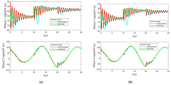
Figure 9.
Control inputs under varied road surface conditions: (a) Control inputs of wheel 1 and wheel 2; (b) control inputs of wheel 3 and wheel 4.
Figure 10 illustrates the approximation performance of the RBF neural network for total disturbances. Figure 10a, Figure 10b, and Figure 10c correspond to the approximation of uncertain disturbances in the , , and directions, respectively. The results indicate that the RBF neural network demonstrates excellent approximation capabilities in all three directions. Even under varying road surface conditions, it can rapidly approximate uncertain disturbance functions and compensate for them in the system, thereby further improving the robustness and control accuracy of the system.
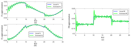
Figure 10.
Approximation performance of the RBF neural network under varied road surface conditions: (a) Approximation performance in the x-direction; (b) approximation performance in the y-direction; and (c) heading angle θ approximation performance.
4.2. Simulation Analysis Under Varied Curvature
This simulation designs a typical reference trajectory with two stages to verify the robustness and dynamic adaptability of different control methods under sudden path curvature changes. The robot tracks a semicircular trajectory with a radius of 3 m in the first 15 s, then switches to a semicircular trajectory with a radius of 1.5 m, forming a sudden change in path curvature. The simulation uses the typical parameters of dry asphalt pavement, and other initial conditions are kept consistent with the previous section to ensure the comparability of experimental results.
The trajectory tracking results are shown in Figure 11. The sliding mode control method based on radial basis function neural networks demonstrates overall excellent performance, effectively suppressing system oscillations caused by path mutations and maintaining high tracking accuracy and smooth dynamic response. The traditional sliding mode control method, with a simpler structure, struggles to adapt to the state disturbances caused by path mutations, leading to obvious overshoot at the curvature change point and poor dynamic performance. This indicates that the neural network-based method exhibits superior control effects in addressing complex nonlinear system characteristics and external disturbances.

Figure 11.
Trajectory tracking with varying curvature.
To objectively evaluate the tracking performance, the relevant performance metrics are calculated based on Equations (22) and (23), with the results presented in Table 4.
Table 4.
IAE and RMSE of circular trajectory with varying curvature.
The tracking performance under varied curvature is illustrated in Figure 12, Figure 13 and Figure 14. Figure 12 depicts the trajectory and velocity tracking in the x-direction and Figure 13 shows the trajectory and velocity tracking in the y-direction. Figure 14 presents the angle and angular velocity tracking in the -direction. During the simulation, at t = 15 s, the reference trajectory of the system abruptly changed from a radius of 3 m to 1.5 m. This imposed significant variations in the corresponding inertial and centrifugal forces acting on the system, creating a pronounced nonlinear disturbance condition. Under this abrupt change scenario, the three control methods exhibited distinct trajectory tracking characteristics.
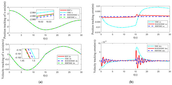
Figure 12.
Tracking performance in the x-direction under varied curvature: (a) Trajectory tracking performance in the x-direction; (b) trajectory tracking error in the x-direction.
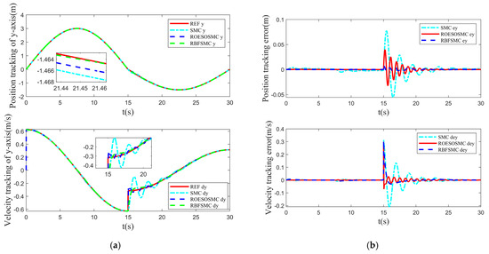
Figure 13.
Tracking performance in the y-direction under varied curvature: (a) Trajectory tracking performance in the y-direction; (b) trajectory tracking error in the y-direction.
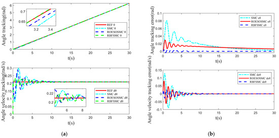
Figure 14.
Heading angle θ tracking performance under varied curvature: (a) Heading angle θ tracking performance; (b) heading angle θ tracking error.
The traditional sliding mode control (SMC) method, due to its inability to effectively compensate for the sudden disturbance and dynamic system changes, exhibited significant tracking errors and transient overshoot, compromising its stability to some extent.
The reduced-order extended state observer-based sliding mode control (ROESOSMC) method enhanced system robustness by dynamically estimating and compensating for system disturbances in real time.
The radial basis function neural network-based sliding mode control (RBFNNSMC) method demonstrated superior tracking accuracy and smoother performance across all directions. Furthermore, during the trajectory transition, the system state underwent more natural transitions without exhibiting violent oscillations.
Figure 15 illustrates the dynamic response of the control input signals for the three control methods during the abrupt curvature change in the trajectory. The simulation results indicate that when the trajectory curvature undergoes an abrupt change at t = 15 s—specifically, switching from a semicircular path with a radius of 3 m to one with a radius of 1.5 m—distinct differences emerge in the input characteristics of the three control methods. Traditional sliding mode control (SMC) exhibits significant input fluctuations at this instant, reflecting its poor adaptability to trajectory variations under non-stationary dynamic conditions, which tends to induce chattering phenomena. The input variations for the reduced-order extended state observer-based sliding mode control (ROESO-SMC) are attenuated near the transition point. In contrast, the radial basis function neural network-based sliding mode control (RBFNN-SMC) demonstrates superior input characteristics, manifesting as a smooth input curve and stable amplitude. This approach significantly suppresses control disturbances induced by the abrupt path change.
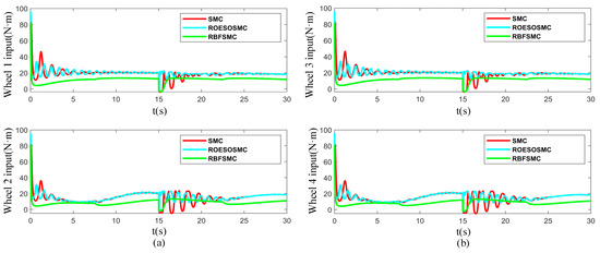
Figure 15.
Control inputs under varied curvature: (a) Control inputs of wheel 1 and wheel 2; (b) control inputs of wheel 3 and wheel 4.
Figure 16 illustrates the approximation performance of the neural network for total disturbances. Figure 16a–c reflect the disturbance approximation in the x-axis, y-axis, and heading angle θ directions, respectively. Simulation results show that the neural network can achieve high-precision approximation of total disturbances in all degrees of freedom, with minimal fluctuation in approximation errors that remain at a low level. This fully demonstrates its excellent online learning ability and adaptive adjustment performance, thereby significantly enhancing the robustness and stability of the control system in complex dynamic environments.
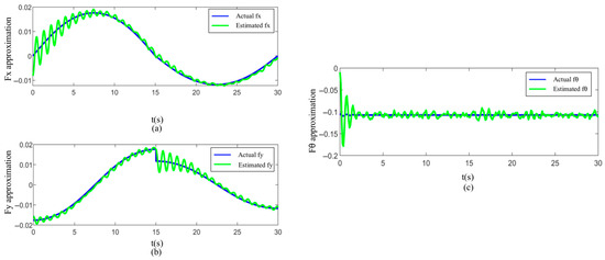
Figure 16.
Approximation performance of the RBF neural network under varied curvature: (a) Approximation performance in the x-direction; (b) approximation performance in the y-direction; and (c) heading angle θ approximation performance.
4.3. Sensitivity Analysis of Controller Parameters
To further verify the structural robustness of the proposed RBF neural network-based sliding mode controller, the controller for the x-direction was selected as a representative case. A sensitivity analysis was conducted on two key structural parameters of the RBF network: the number of nodes N and the basis function width . Simulation experiments were performed under variable-curvature reference trajectory conditions. While keeping all other controller parameters and experimental settings constant, the Integral Absolute Error (IAE) and Root Mean Square Error (RMSE) were employed as performance metrics to analyze the controller’s response characteristics under different parameter configurations.
Firstly, with the basis function width fixed at = 5.0, the number of nodes was set to 3, 5 (default), and 7. The experimental results are summarized in Table 5. The findings indicate that with only three nodes, the network’s approximation capability was insufficient, leading to significantly larger errors. When the number of nodes was set to five, both the IAE and RMSE reached their optimal values. Increasing the node count further to seven resulted in a slight increase in error. Analysis suggests that while a higher number of nodes enhances the model’s expressive power, it concurrently increases network complexity. This elevates the risk of overfitting and slows down the adaptive weight adjustment process, ultimately impairing the system’s generalization capability. Considering the trade-off between approximation accuracy and computational complexity, setting the number of nodes to five achieves a favorable performance balance.
Table 5.
Effect of the number of nodes on control performance.
Subsequently, with the number of nodes fixed at five, the Gaussian basis function width parameter was adjusted to 2.0, 5.0 (default), and 8.0 to evaluate its impact on control precision. The comparative results are presented in Table 6. The experiments reveal that variations in the basis function width exerted a relatively minor influence on the error metrics, indicating that the controller exhibits substantial robustness to this parameter. When the width was set too small, the Gaussian functions became overly sharp, resulting in a narrow local response range. Conversely, an excessively large width led to flattened function responses, potentially degrading approximation accuracy. The default value = 5.0 achieved an optimal balance between the approximation range and function sensitivity, delivering the best performance.
Table 6.
Effect of basis function width on control performance.
In summary, the proposed RBF sliding mode controller demonstrates favorable control accuracy and stability across the evaluated variations in structural parameters, exhibiting strong robustness to both the number of nodes and the basis function width. Given the identical controller configuration for the Y-direction and angular direction controllers, the conclusions drawn from this analysis possess significant representativeness. Consequently, these findings can be extended to reflect the overall control strategy’s adaptability to parameter configuration variations.
5. Experimental Validation
5.1. System Architecture
The system architecture, illustrated in Figure 17, comprises four primary components: the mobile robot platform, the controller, sensors, and the Human–Machine Interface (HMI). Functioning as the core element, the controller receives commands from the HMI. By leveraging real-time attitude and position data acquired by the sensors, it computes motion commands to drive the robot. The sensor module continuously monitors operational states, feeding back information for closed-loop control. The HMI facilitates data exchange between the host computer and the control system, enabling status monitoring, parameter configuration, and remote debugging. These components operate synergistically via stable communication links, forming a closed-loop control structure that enhances real-time system performance and reliability in complex environments.
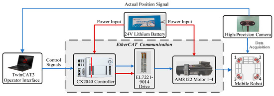
Figure 17.
Block diagram of the omnidirectional mobile robot prototype system.
To validate the practical implementability of the controller, the control algorithm was deployed and tested on the Beckhoff CX2040 industrial PC platform. This platform features an Intel® Core™ i7 quad-core processor running the TwinCAT 3 real-time operating system. With the control cycle set to 10 ms, the measured average computation time per cycle was 2.3 ms, with a maximum of 3.1 ms. This is significantly below the real-time control threshold, confirming suitability for embedded deployment. The compact structure of the designed RBF sliding mode controller, whose core computations involve only exponential functions, weighted summation, and weight updates, results in low computational complexity and minimal resource utilization. This ensures excellent adaptability to embedded platforms.
Following successful controller deployment and real-time performance verification, two sets of representative simulation experiments were designed to further evaluate the robustness and adaptability of the proposed control method under practical operating conditions. These tests specifically address variable ground conditions and variable-curvature reference trajectories. By simulating external disturbances and variations in trajectory complexity, the controller’s dynamic response performance and trajectory tracking accuracy in non-ideal environments were systematically analyzed. This provides substantive experimental evidence to validate its engineering applicability.
5.2. Experiment Under Varied Road Surface Conditions
The trajectory tracking effect of the robot under varied road conditions is shown in Figure 18. The desired trajectory is a circle with a radius of 1 m (marked by a red dashed line). In the experiment, the robot moves along the preset trajectory at 0.2 m/s, and the blue solid line represents the actual movement trajectory. The results show that on smooth floor tiles, with less resistance, the robot can move along the desired trajectory more accurately. When the robot enters the rough blanket area, the movement resistance increases, external interferences grow, and the uneven blanket surface causes vibrations and deviations during movement, leading to slight offsets in the actual trajectory. Compared with the smooth floor tile area, the tracking error of the robot on the blanket increases slightly, but it can still maintain good trajectory tracking performance.
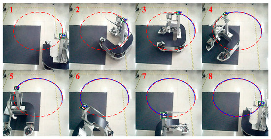
Figure 18.
Trajectory tracking results under varied road conditions.
Eight key sampling points were selected along the preset circular target trajectory starting from the robot’s initial position. The camera positioning system was used to collect real-time actual position information of these eight sampling points during the robot’s movement, including the x-axis position, y-axis position, and heading angle θ. Subsequently, the collected actual data were carefully compared and analyzed with the desired x-axis position, y-axis position, and heading angle θ at the corresponding moments. The comparison results are detailed in Table 7, Table 8 and Table 9. Experimental data show that the mobile robot has small errors between the actual pose and the desired pose at each sampling point throughout the trajectory tracking process. The maximum position errors in the x-axis and y-axis directions do not exceed 0.8 cm, and the maximum error in the heading angle θ is constrained to within 0.04 rad. The experimental results verify the high precision and robustness of the method.
Table 7.
Comparison of desired and actual x-axis values under varied road surface conditions.
Table 8.
Comparison of desired and actual y-axis values under varied road surface conditions.
Table 9.
Comparison of desired and actual yaw angles under varied road surface conditions.
5.3. Experiment Under Varied Curvature
The trajectory tracking effect of the robot when the trajectory curvature changes is shown in Figure 19. The desired trajectory transitions from a circle with a radius of 1 m to a circle with a radius of 0.5 m (the red dashed line marks the desired trajectory, and the blue solid line represents the actual movement trajectory). The results show that the sudden change in trajectory curvature initially causes a large tracking error in the robot. However, with the adjustment and correction of the control system, the error decreases rapidly and finally stabilizes within a small range, being relatively close to the desired trajectory.
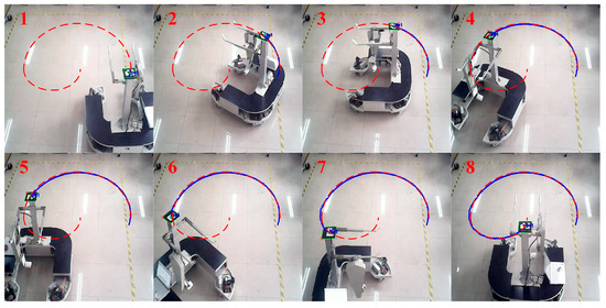
Figure 19.
Trajectory tracking results under varied curvature conditions.
During the robot’s movement from the starting position to the end of the target path, eight key sampling points were uniformly selected along the preset trajectory, and a high-precision camera positioning system was used to collect real-time actual pose information at each sampling point, including the x-axis position, y-axis position, and heading angle θ. The collected actual poses were then compared with the expected poses at each corresponding sampling point to quantitatively evaluate the tracking error and the performance of the control method. The specific comparison results are detailed in Table 10, Table 11 and Table 12.
Table 10.
Comparison of desired and actual x-axis values under varied curvature.
Table 11.
Comparison of desired and actual y-axis values under varied curvature.
Table 12.
Comparison of desired and actual yaw angles under varied curvature.
Experimental data show that the mobile robot has small errors between the actual and expected poses at each sampling point throughout the trajectory tracking process. Specifically, the maximum position errors in the x-axis and y-axis directions do not exceed 1.2 cm, and the maximum error in the heading angle θ is controlled within 0.05 rad. These results verify that the proposed method exhibits high tracking accuracy and good robustness under curvature change conditions.
6. Conclusions
This paper proposes a method combining radial basis function (RBF) neural networks with sliding mode control (SMC). The method leverages RBF neural networks to approximate and compensate for the total disturbances in sliding mode control while employing a hyperbolic tangent function instead of the traditional sign function. This approach effectively reduces chattering in sliding mode control and accurately estimates the uncertainties within the system model. By integrating the advantages of sliding mode control and RBF neural networks, the proposed controller achieves excellent control performance without requiring complete system information, thereby enhancing its applicability in various scenarios.
Additionally, the use of online adaptive RBF network control, based on Lyapunov stability analysis, avoids the common issue of traditional gradient descent methods becoming trapped in local optima when adjusting the neural network weights. Simulation and experimental results demonstrate the significant superiority and effectiveness of the proposed method.
Author Contributions
Conceptualization, C.Y.; methodology, H.L.; software, H.L. and S.T.; writing—original draft preparation, H.L.; writing—review and editing, S.T. and S.Y.; supervision, C.Y. and S.Y.; project administration, C.Y. All authors have read and agreed to the published version of the manuscript.
Funding
This research was funded by Project of Liaoning Provincial Education Department, China (Nos. 20240213 and 20240153; Funder ID: 10.13039/501100013099).
Data Availability Statement
The original data contributions presented in the study are included in the article, further inquiries can be directed to the corresponding author.
Conflicts of Interest
The authors declare no conflicts of interest.
References
- Sun, Z.; Hu, S.; Xie, H.; Li, H.; Zheng, J.; Chen, B. Fuzzy adaptive recursive terminal sliding mode control for an agricultural omnidirectional mobile robot. Comput. Electr. Eng. 2023, 105, 108529. [Google Scholar] [CrossRef]
- Patruno, C.; Renò, V.; Nitti, M.; Mosca, N.; Di Summa, M.; Stella, E. Vision-based omnidirectional indoor robots for autonomous navigation and localization in manufacturing industry. Heliyon 2024, 10, 26042. [Google Scholar] [CrossRef] [PubMed]
- Yildiz, I. A Low-Cost and Lightweight Alternative to Rehabilitation Robots: Omnidirectional Interactive Mobile Robot for Arm Rehabilitation. Arab. J. Sci. Eng. 2018, 43, 1053–1059. [Google Scholar] [CrossRef]
- Ren, C.; Ma, S. Generalized proportional integral observer based control of an omnidirectional mobile robot. Mechatronics 2015, 26, 36–44. [Google Scholar] [CrossRef]
- Ren, C.; Ding, Y.; Li, X.; Zhu, X.; Ma, S. Extended State Observer Based Robust Friction Compensation for Tracking Control of an Omnidirectional Mobile Robot. J. Dyn. Syst. Meas. Control 2019, 141, 101001. [Google Scholar] [CrossRef]
- Ren, C.; Ding, Y.; Ma, S. A structure-improved extended state observer based control with application to an omnidirectional mobile robot. ISA Trans. 2020, 101, 335–345. [Google Scholar] [CrossRef]
- Jeong, S.; Chwa, D. Sliding-Mode-Disturbance-Observer-Based Robust Tracking Control for Omnidirectional Mobile Robots With Kinematic and Dynamic Uncertainties. IEEE/ASME Trans. Mechatron. 2021, 26, 741–752. [Google Scholar] [CrossRef]
- Ren, C.; Ding, Y.; Ma, S.; Hu, L.; Zhu, X. Passivity-based tracking control of an omnidirectional mobile robot using only one geometrical parameter. Control Eng. Pract. 2019, 90, 160–168. [Google Scholar] [CrossRef]
- Ye, C.; Shao, J.; Liu, Y.; Yu, S. Fuzzy active disturbance rejection control method for an omnidirectional mobile robot with MY3 wheel. IR 2023, 50, 706–716. [Google Scholar] [CrossRef]
- Shahgholian, S.; Akhavan, M.; Kamrani, V.; Ganjefar, S. Design an omnidirectional autonomous mobile robot based on non-linear optimal control to track a specified path. IET Control Theory Appl. 2024, 18, 1200–1209. [Google Scholar] [CrossRef]
- Ren, C.; Jiang, H.; Mu, C.; Ma, S. Conditional Disturbance Negation Based Control for an Omnidirectional Mobile Robot: An Energy Perspective. IEEE Robot. Autom. Lett. 2022, 7, 11641–11648. [Google Scholar] [CrossRef]
- Zhang, L.; Kim, J.; Sun, J. Energy Modeling and Experimental Validation of Four-Wheel Mecanum Mobile Robots for Energy-Optimal Motion Control. Symmetry 2019, 11, 1372. [Google Scholar] [CrossRef]
- Al Mamun, M.; Nasir, M.; Khayyat, A. Embedded System for Motion Control of an Omnidirectional Mobile Robot. IEEE Access 2018, 6, 6722–6739. [Google Scholar] [CrossRef]
- Ren, C.; Li, C.; Hu, L.; Li, X.; Ma, S. Adaptive model predictive control for an omnidirectional mobile robot with friction compensation and incremental input constraints. Trans. Inst. Meas. Control 2022, 44, 835–847. [Google Scholar] [CrossRef]
- Karras, G.; Fourlas, G. Model Predictive Fault Tolerant Control for Omni-directional Mobile Robots. J. Intell. Robot Syst. 2020, 97, 635–655. [Google Scholar] [CrossRef]
- El-Sayyah, M.; Saad, M.; Saad, M. Enhanced MPC for Omnidirectional Robot Motion Tracking Using Laguerre Functions and Non-Iterative Linearization. IEEE Access 2022, 10, 118290–118301. [Google Scholar] [CrossRef]
- Wu, H.; Karkoub, M. Frictional forces and torques compensation based cascaded sliding-mode tracking control for an uncertain omnidirectional mobile robot. Meas. Control 2022, 55, 178–188. [Google Scholar] [CrossRef]
- Feng, X.; Wang, C. Robust Adaptive Terminal Sliding Mode Control of an Omnidirectional Mobile Robot for Aircraft Skin Inspection. Int. J. Control Autom. Syst. 2021, 19, 1078–1088. [Google Scholar] [CrossRef]
- Sun, Z.; Hu, S.; He, D.; Zhu, W.; Xie, H.; Zheng, J. Trajectory-tracking control of Mecanum-wheeled omnidirectional mobile robots using adaptive integral terminal sliding mode. Comput. Electr. Eng. 2021, 96, 107500. [Google Scholar] [CrossRef]
- Ren, C.; Li, X.; Yang, X.; Ma, S. Extended State Observer-Based Sliding Mode Control of an Omnidirectional Mobile Robot With Friction Compensation. IEEE Trans. Ind. Electron. 2019, 66, 9480–9489. [Google Scholar] [CrossRef]
- Abiyev, R.; Akkaya, N.; Gunsel, I. Control of Omnidirectional Robot Using Z-Number-Based Fuzzy System. IEEE Trans. Syst. Man. Cybern Syst. 2019, 49, 238–252. [Google Scholar] [CrossRef]
- Chiu, C.; Lin, C. Control of an omnidirectional spherical mobile robot using an adaptive Mamdani-type fuzzy control strategy. Neural Comput. Appl. 2018, 30, 1303–1315. [Google Scholar] [CrossRef]
- Yu, D.; Chen, C.; Xu, H. Fuzzy Swarm Control Based on Sliding-Mode Strategy With Self-Organized Omnidirectional Mobile Robots System. IEEE Trans. Syst. Man. Cybern Syst. 2022, 52, 2262–2274. [Google Scholar] [CrossRef]
- Cao, G.; Zhao, X.; Ye, C.; Yu, S.; Li, B.; Jiang, C. Fuzzy adaptive PID control method for multi-mecanum-wheeled mobile robot. J. Mech. Sci. Technol. 2022, 36, 2019–2029. [Google Scholar] [CrossRef]
- Feng, X.; Wang, C. Adaptive neural network tracking control of an omnidirectional mobile robot. Proc. Inst. Mech. Eng. Part I J. Syst. Control Eng. 2023, 237, 375–387. [Google Scholar] [CrossRef]
- Da Silva Lima Moreira, G.; Bessa, W. Accurate trajectory tracking control with adaptive neural networks for omnidirectional mobile robots subject to unmodeled dynamics. J. Braz. Soc. Mech. Sci. Eng. 2023, 45, 48. [Google Scholar] [CrossRef]
- Lu, X.; Zhang, X.; Zhang, G.; Fan, J.; Jia, S. Neural network adaptive sliding mode control for omnidirectional vehicle with uncertainties. ISA Trans. 2019, 86, 201–214. [Google Scholar] [CrossRef]
- Achirei, S.; Mocanu, R.; Popovici, A.; Dosoftei, C. Model-Predictive Control for Omnidirectional Mobile Robots in Logistic Environments Based on Object Detection Using CNNs. Sensors 2023, 23, 4992. [Google Scholar] [CrossRef]
- Qin, P.; Zhao, T.; Dian, S. Interval type-2 fuzzy neural network-based adaptive compensation control for omni-directional mobile robot. Neural Comput. Appl. 2023, 35, 11653–11667. [Google Scholar] [CrossRef]
- Zhao, T.; Qin, P.; Dian, S.; Guo, B. Fractional order sliding mode control for an omni-directional mobile robot based on self-organizing interval type-2 fuzzy neural network. Inf. Sci. 2024, 654, 119819. [Google Scholar] [CrossRef]
- Yun, C.; Sin, Y.; Ri, H.; Jo, K. Trajectory tracking control of a three-wheeled omnidirectional mobile robot using disturbance estimation compensator by RBF neural network. J. Braz. Soc. Mech. Sci. Eng. 2023, 45, 432. [Google Scholar] [CrossRef]
- Niu, Z.-J.; Zhang, P.; Cui, Y.-J.; Zhang, J. PID control of an omnidirectional mobile platform based on an RBF neural network controller. IR 2022, 49, 65–75. [Google Scholar] [CrossRef]
- Yan, X.; Wang, H. Operational control with set-points tuning—Application to mobile robots. Intell. Robot 2023, 3, 113–130. [Google Scholar] [CrossRef]
- Pan, C.; Huang, H.; Chen, C.; Wu, L.; Xiao, J. Neuro-adaptive command-filtered backstepping control of uncertain flexible-joint manipulators with input saturation via output. Sci. Rep. 2025, 15, 17254. [Google Scholar] [CrossRef]
- Ye, C.; Sun, Y.; Yu, S.; Ding, J.; Jiang, C. Motion optimization of an omnidirectional mobile robot with MY wheel based on contact mechanics. IR 2022, 49, 962–972. [Google Scholar] [CrossRef]


Disclaimer/Publisher’s Note: The statements, opinions and data contained in all publications are solely those of the individual author(s) and contributor(s) and not of MDPI and/or the editor(s). MDPI and/or the editor(s) disclaim responsibility for any injury to people or property resulting from any ideas, methods, instructions or products referred to in the content. |
© 2025 by the authors. Licensee MDPI, Basel, Switzerland. This article is an open access article distributed under the terms and conditions of the Creative Commons Attribution (CC BY) license (https://creativecommons.org/licenses/by/4.0/).