MCMBAN: A Masked and Cascaded Multi-Branch Attention Network for Bearing Fault Diagnosis

Abstract

In recent years, deep learning methods have made breakthroughs in the field of rotating equipment fault diagnosis, thanks to their powerful data analysis capabilities. However, the vibration signals usually incorporate fault features and background noise, and these features may be scattered over multiple frequency levels, which increases the complexity of extracting important information from them. To address this problem, this paper proposes a Masked and Cascaded Multi-Branch Attention Network (MCMBAN), which combines the Noise Mask Filter Block (NMFB) with the Multi-Branch Cascade Attention Block (MBCAB), and significantly improves the noise immunity of the fault diagnostic model and the efficiency of fault feature extraction. NMFB novelly combines a wide convolutional layer and a top k neighbor self-attention masking mechanism, so as to efficiently filter unnecessary high-frequency noise in the vibration signal. On the other hand, MBCAB strengthens the interaction between different layers by cascading the convolutional layers of different scales, thus improving the recognition of periodic fault signals and greatly enhancing the diagnosis accuracy of the model when processing complex signals. Finally, the time–frequency analysis technique is employed to explore the internal mechanisms of the model in depth, aiming to validate the effectiveness of NMFB and MBCAB in fault feature recognition and to improve the feature interpretability of the proposed modes in fault diagnosis applications. We validate the superior performance of the network model in dealing with high-noise backgrounds by testing it on a standard bearing dataset from Case Western Reserve University and a self-constructed composite bearing fault dataset, and the experimental results show that its performance exceeded six of the top current fault diagnosis techniques.

1. Introduction

Rotating machinery plays a pivotal role in modern industrial systems, serving as critical equipment across various production environments, including bearing assemblies, fluid compression devices, power transmission mechanisms, and aerospace propulsion units [1,2]. Among these, rolling-element bearings and gear transmission systems are fundamental functional components of rotating machinery, whose operational integrity directly influences overall system reliability. Any malfunction can lead to unplanned downtime, resulting in significant production losses and potential safety hazards. In recent years, advancements in intelligent algorithms and signal processing techniques have spurred growing interest in vibration-based condition monitoring and fault diagnosis methods for bearings [3,4]. These diagnosis techniques extract fault information from a large amount of monitoring data and are suitable for application in complex environments where models are difficult to define precisely [5].

Recently, the integration of signal processing and deep learning technologies has significantly advanced intelligent fault diagnosis of rolling bearings. Particularly, deep learning has shown exceptional performance in the field of pattern recognition, leading to its growing popularity in fault diagnosis technologies. These methods examine raw data by employing neural networks and can automate the extraction of important features, minimizing the demand for traditional data preprocessing and expertise. Convolutional Neural Networks (CNNs) have demonstrated their superiority in several fields, and their application in bearing fault diagnosis is rapidly expanding [6,7]. For example, Song et al. [8] extracted high-dimensional and temporal features from raw vibration signals through CNNs to accurately identify fault characteristics and enhance diagnosis accuracy. Similarly, Ruan et al. [9] leveraged fault cycles corresponding to various fault types and shaft rotation frequencies to establish the CNN input size and then used the signal length to define the kernel size of the CNN. In addition, the study by Jie et al. [10] was the first to design a systematic degradation testing method for electric vehicle bearings considering circulating bearing currents. It provided a data acquisition and analysis platform for scenarios where electrical and mechanical loads are coupled, which are common in real industrial environments. This significantly improves the realism of the data and the applicability of diagnostic methods. Nevertheless, in complex data environments, especially under high noise levels, the distinctions across various types of bearing faults can be very subtle, posing a challenge to the discriminative ability of CNNs. The considerable level of similarity and variability in fault diagnosis presents certain difficulties in precisely identifying particular types of faults.

Attention mechanisms have been successfully incorporated into deep learning models, greatly enhancing the feature interpretability of models in various fields. Attention mechanisms enhance the accuracy of fault diagnosis by assigning weights to input data segments, enabling the model to focus on anomalies within vibration patterns [11]. Furthermore, the model is able to recognize complex patterns and long-term dependencies in the data, given that these mechanisms produce outputs by concentrating on certain elements of the input sequence. Several deep learning architectures have been developed to tackle complex fault diagnosis challenges by utilizing these features. For example, Zhou et al. [12] designed a CNN fault diagnosis method for rolling bearings based on a frequency attention mechanism, which effectively addressed the issue of poor diagnosis performance under the interference of strong noise. Cui et al. [13] incorporated self-attention as the network’s backbone and used contrastive (comparative) learning on positive samples to extract key features from unlabeled fault data. Zhong et al. [14] proposed a weighted domain adaptive network with residual denoising and multi-scale attention. This network integrates residual denoising and multi-scale attention modules to enhance domain adaptation performance even when significant domain interference exists. Li et al. [15] introduced a hybrid attention mechanism to improve the neural network’s ability to extract effective feature information, addressing challenges related to small and imbalanced samples under noisy conditions. Despite the exciting research opportunities in fault diagnosis, the integration of attention with neural networks lacks unified guidelines for attention structure design, and most models have not yet established an explicit connection with fault processes [16,17].

Although current deep learning methods have shown significant advantages in bearing fault diagnosis, they still face major challenges in real industrial applications due to the lack or scarcity of fault data. In recent years, many studies have proposed innovative solutions to address this issue, such as physics-driven domain adaptation and zero-shot learning approaches. Sobie et al. [18] proposed a simulation-driven machine learning method that uses bearing dynamic models to generate high-fidelity simulated fault data. This helps to overcome the shortage of real data and enables accurate fault classification. In addition, Matania et al. [19] introduced a zero-fault-shot learning method, which combines physical simulation with a small amount of real data. By projecting fault signals into an invariant feature space, this approach allows for effective fault type identification even without real fault samples. These studies offer new perspectives for addressing data scarcity in bearing diagnosis and promote the practical application of fault diagnosis methods in real industrial settings.

In summary, although deep learning technologies have achieved significant achievements in the fault diagnosis of bearing, several key challenges remain in practical applications: (1) While deep neural networks, primarily CNNs, can automatically extract features from vibration data, these models often struggle to differentiate which features are important fault indicators and which are just environmental noise. (2) The occurrence of bearing faults is usually complex, and damage at multiple locations can lead to overlapping features, which makes it possible for models to mistakenly classify multiple faults as more common single faults. (3) The invisibility of the decision-making processes and internal mechanisms of deep neural networks typically makes them inappropriate for widespread application in industries that demand robust auditing.

In this paper, a new Masked and Cascaded Multi-Branch Attention Network (MCMBAN) is proposed. Initially, a Noise Mask Filter Block (NMFB) is constructed to efficiently filter and eliminate high-frequency noise from the signal by using the wide convolutional layer and the top k neighbor self-attention masking mechanism. Subsequently, a Multi-Branch Cascade Attention block (MBCAB) was designed to deeply analyze the correlation between multiple time-scale fault features using attention cascade layers. Finally, these two core blocks are combined to form an efficient and interpretable fault diagnosis model. Moreover, the feature interpretability of the model is further enhanced by applying a continuous wavelet transform to analyze the variation in signals within the model. The main outcomes of this research include the following:

(1) The proposed MCMBAN model utilizes NMFB to distinguish and filter out high-frequency noise features, while MBCAB helps the model to identify and differentiate the relationships among different fault information. (2) The designed framework based on MCMBAN demonstrates effectiveness in handling high levels of noise backgrounds and complex fault situations while also exhibiting superior adaptability and diagnosis performance. (3) Through time–frequency analysis, the fluctuations of non-periodic signals in the model are characterized, which enhances the feature interpretability of the model in fault diagnosis applications.

The structure of this article is organized as follows: Section 2 provides the comprehensive description of the composition of the MCMBAN model, including the detailed design of NMFB and MBCAB. Section 3 validates the fault diagnosis results of the method and explores the feature interpretability. Section 4 summarizes the experimental and research results.

2. Method Overview

Rolling bearings in manufacturing processes often exhibit several types of failures, which can manifest similar features in vibration signals; thus, fault diagnosis systems are susceptible to misclassifying complex faults as common single fault types [20]. 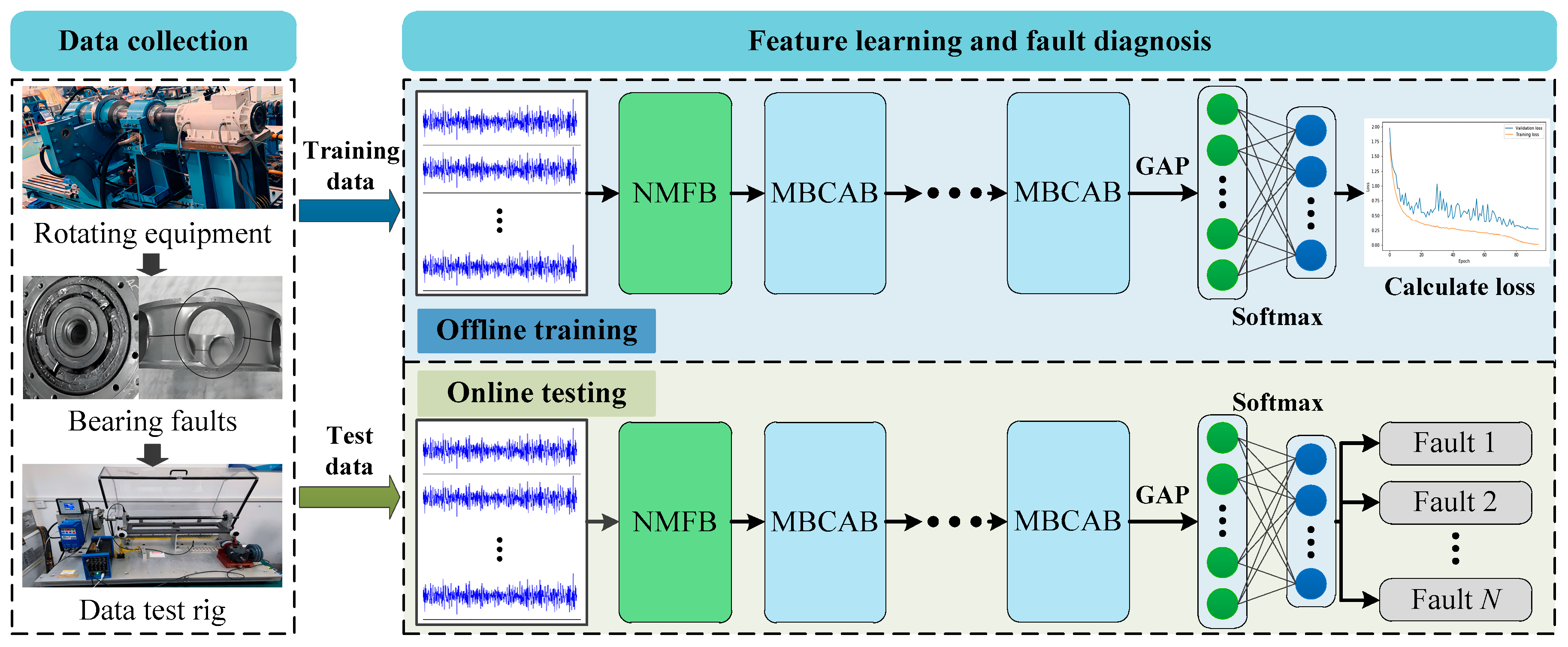In addition, the masking effect of high-frequency environmental noise can impair the ability of the diagnosis system to identify real fault signals [21]. In order to tackle these difficulties, this paper proposes a novel Interpretable Multi-Branch Cascade Network (MCMBAN) for fault diagnosis in noisy environments. The structure of MCMBAN is illustrated in Figure 1, where the system acquires the raw vibration data from the bearing acquisition equipment and feeds it into MCMBAN. MCMBAN consists of two key feature learning blocks: Noise Mask Filter Block (NMFB) and Multi-Branch Cascade Attention Block (MBCAB). NMFB effectively filters out high-frequency noise by using a wide convolution with a top k neighbor self-attention masking mechanism, while MBCAB explores the interrelationships between different fault types through inter-layer interactions. Ultimately, these features are compressed into one-dimensional features by means of a global average pooling (GAP) layer, as well as fault category mapping by means of a softmax function.

2.1. Noise Mask Filter Block (NMFB)

During the operation of bearings, internal friction and structural vibrations inevitably generate substantial background noise, which often masks the critical fault-related information embedded in the vibration signals. To effectively mitigate the influence of such noise, contemporary deep learning-based fault diagnosis methods commonly employ wide convolutional (Wide Convolution) structures with large convolutional kernels. By covering a broader temporal receptive field, large kernels exhibit stronger responsiveness to low-frequency components of the signals, thereby contributing to the suppression of high-frequency noise.

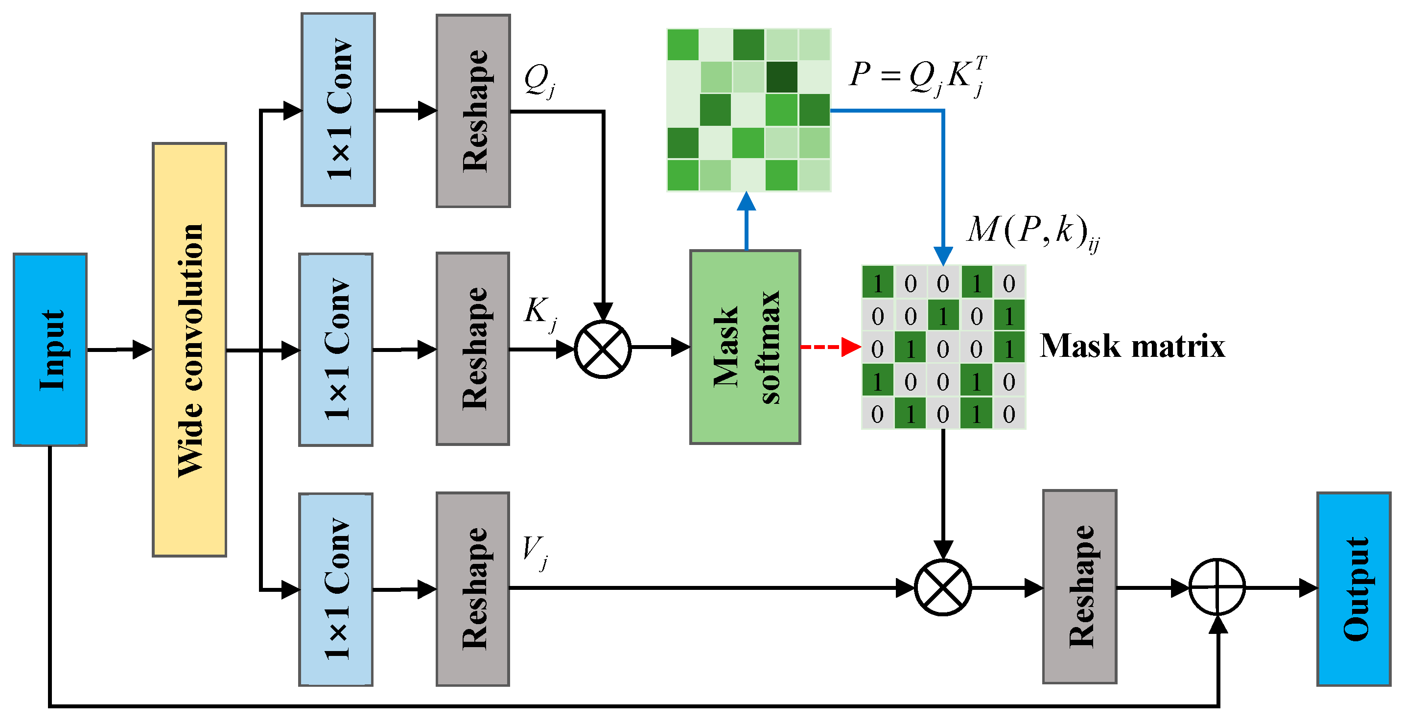
However, bearing faults are typically characterized by significant high-frequency features. Traditional wide convolution layers, while attenuating high-frequency noise, may simultaneously suppress these critical fault frequencies, leading to a degradation in diagnostic sensitivity. To address this challenge, this paper proposes a Noise Mask Filter Block (NMFB). Figure 2 illustrates the structure of NMFB.

Within NMFB, the wide convolution operation is integrated with a self-attention mechanism to explore the internal correlations among the extracted features. Through the top k neighbor self-attention masking mechanism, the network can adaptively analyze the interdependencies and relative importance of different features, dynamically enhancing fault-relevant information while suppressing irrelevant or redundant noise components. This enables fine-grained optimization of the feature representations obtained by the wide convolution. Compared to conventional wide convolution approaches, NMFB achieves superior noise suppression while effectively preserving key high-frequency fault features, thereby significantly improving both diagnostic accuracy and robustness. In the following sections, we will provide a comprehensive explanation of the construction, underlying mechanisms, and application effectiveness of the proposed NMFB within the context of fault diagnosis tasks.

Step 1: Wide convolutional layers can suppress high-frequency anomalous information in features, so a wide convolutional layer is used to process the original signal, following the formula below:

$$y=F(x,G)$$

(1)

where $F(·)$ is the wide convolutional layer operation, $x$ is the input signal, $G$ refers to the convolution kernel parameter, $y$ represents the convolution output, $y=[y_1,y_2,\cdots ,y_C]$, and the number of channels is $C$.

Step 2: Queries (Q), keys (K), and values (V) are generated by three 1 × 1 convolution operations and shape transformations, which will be used to calculate the correlation of features in $y_i$ following the formula below:

$$Q_j=W_j^Q\ast y_i$$

(2)

$$K_j=W_j^K\ast y_i$$

(3)

$$V_j=W_j^V\ast y_i$$

(4)

where $W_j^Q$, $W_j^K$, and $W_j^V$ represent the convolutional weights of the j-th head. Then, the similarity between $Q_j$ and $K_j$ is computed to obtain the attention score. The formula is as follows:

$$P=Q_j{K}_j^T$$

(5)

where $P$ represents the similarity matrix. Since noise typically manifests as globally low-correlated random fluctuations in signals, while fault features exhibit locally strong correlations, mask screening can help the model suppress low-correlation noise connections and focus on fault-sensitive features with strong correlations by retaining high-similarity feature connections. To this end, this paper filters out elements in the similarity matrix that fall below a threshold using a mask, retaining only the k neighbors most relevant to the current feature. For each row of the similarity matrix $P$, the values are sorted in descending order, and only the top k largest values are retained, with the rest set to zero. The formula is as follows:

$$M{(P,k)}_{ij}=\left\{\begin{array}{c}{P}_{ij}if{P}_{ij}\ge \mathrm{threshold}\\ 0if{P}_{ij}<\mathrm{threshold}\end{array}\right.$$

(6)

Afterwards, the softmax function normalizes all similarity values into a probability distribution, so that the output of each position is a weighted sum of all position values following the formula below:

$$A_j=\mathrm{softmax}({\displaystyle \frac{M{(P,k)}_{ij}}{\sqrt{d_k}}})$$

(7)

$$z_j=A_j{V}_j$$

(8)

where $\sqrt{d_k}$ is the dimension of $K_j$, which is used to scale the dot product result. $A_j$ denotes the attention weights, and $z_j$ denotes the weight-calibrated feature of the j-th head. Finally, the outputs of all heads are combined as follows:

$$Z=\mathrm{Concat}(z_1,z_2,\cdots ,z_h)W^o+x$$

(9)

where $W^o$ denotes the weight of the output linear transformation, which is applied to combine the outputs of the multiple heads. $Z$ denotes the output of the top k neighbor self-attention masking mechanism, and the attention masking mechanism dynamically adjusts the contribution to enhance the representation of features relevant to faults while simultaneously suppressing noise.

In summary, by introducing the top k neighbor self-attention masking mechanism, NMFB can process information in parallel across multiple representation subspaces, which improves the model’s ability to distinguish between faulty and noisy features in the signal. The top k neighbor self-attention masking mechanism allows the model to capture different feature spaces information, thereby increasing its capacity to identify complex patterns. This is especially well-suited for applications such as bearing fault diagnosis, where absolute sensitivity and accuracy are crucial.

2.2. Multi-Branch Cascade Attention Block (MBCAB)

Bearing failures often generate distinctive periodic impulses in the vibration data, with significant correlations between these impulses. Through detailed analysis of these correlations, the degree of the type of fault can be effectively identified. Therefore, this article designs a Multi-Branch Cascade Attention Block (MBCAB), which helps the network to capture pulse correlation information in vibration signals. 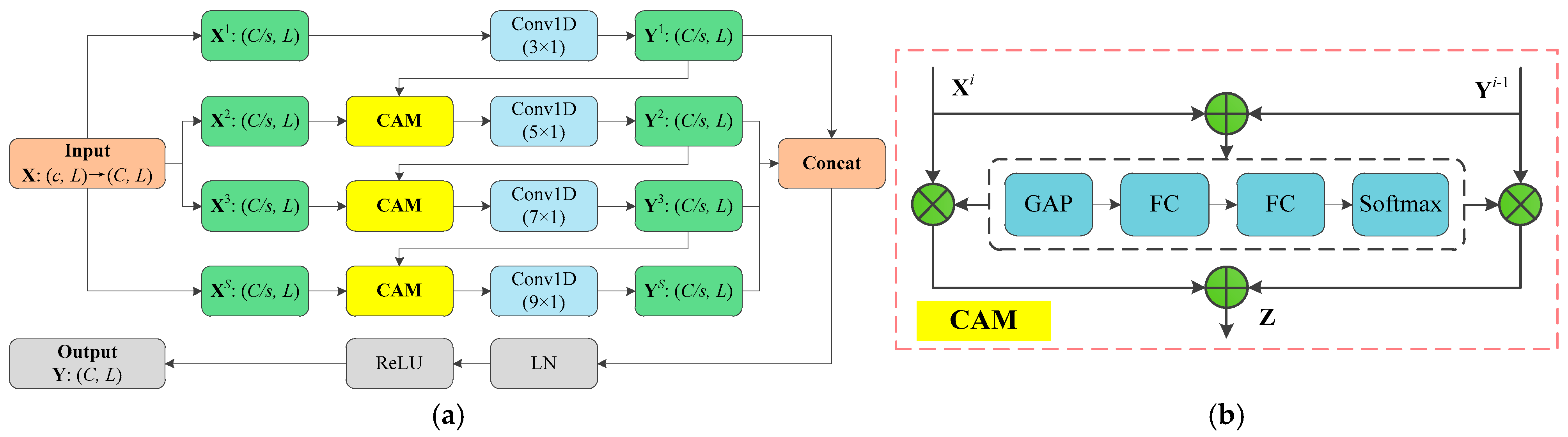Figure 3a illustrates the structure of MBCAB, which principally consists of cascaded attention mechanism (CAM) and multi-scale convolution layers. The details of MBCAB are introduced as follows.

Step 1: Multi-branch feature segmentation

Initially, a 1 × 1 convolutional layer is employed to adjust the number of channels in the input feature matrix to $C$. The adjusted features can be expressed as $\mathbf{X}\in {\mathrm{R}}^{C\times L}$. Subsequently, $\mathbf{X}$ is divided along the channel dimension into $s$ branch features ${\mathbf{X}}^i$, and each branch feature contains $C/s$ channels, where $1\le i\le s$. This division aids the model in independently extracting information from different branch features, following the formula below:

$${\mathbf{X}}^i={[{\mathbf{X}}_1^i,{\mathbf{X}}_2^i,\cdots ,{\mathbf{X}}_{C/s}^i]}^{\mathrm{T}}$$

(10)

where ${\mathbf{X}}_{C/s}^i$ is the i-th feature subset’s channel features.

Step 2: Multi-branch feature extraction

A convolutional kernel of varying sizes is first applied to each branch feature ${\mathbf{X}}^i$, gradually increasing from small to large, in order to capture features ranging from fine-grained to coarse-grained. Subsequently, the cascade attention structure is utilized to facilitate the interaction among several convolutional layers, allowing the output of the previous layer to influence the input of the next layer, thereby enhancing the correlation and continuity among features. The structure of CAM is shown in Figure 3b. Assuming that ${\mathbf{Y}}^{i-1}$ is the output features of the previous layer and ${\mathbf{X}}^i$ is the input features of the next layer, the cascade attention simultaneously processes ${\mathbf{Y}}^{i-1}$ and ${\mathbf{X}}^i$. First, ${\mathbf{Y}}^{i-1}$ and ${\mathbf{X}}^i$ are fused by element-wise addition to obtain the fused feature ${\mathbf{Z}}^i$. Then, the feature ${\mathbf{Z}}^i$ is processed through a GAP layer, the channel aggregation layer, and the softmax layer to obtain the weight features ${\mathbf{b}}_1$ and ${\mathbf{b}}_2$ of the two features. After that, the weight features are multiplied with ${\mathbf{Y}}^{i-1}$ and ${\mathbf{X}}^i$, respectively, to calibrate the output features of the previous layer and the input features of the next layer. Finally, the calibrated features are merged to produce the output features of the cascade attention layer. To summarize, the output features of each convolutional layer are combined with the input of the adjacent layers and processed through larger convolutional layers to achieve efficient interactions among the layers.

The multi-branch feature extraction part of the MBCAB module introduces convolution kernels of multiple sizes, with the aim of extracting both local and global features of the fault signal across different time scales. MBCAB uses four convolution kernels of sizes 3 × 1, 5 × 1, 7 × 1, and 9 × 1 to extract fault signal features at different time scales. The 3 × 1 convolution kernel has the narrowest receptive field and is used to extract high-frequency transient features, helping the model identify minor faults, local perturbations, and anomalies. The 5 × 1 convolution kernel balances the local and periodic structure of the vibration signal, assisting the model in extracting periodic impact features for moderate damage. The 7 × 1 and 9 × 1 kernels cover larger receptive fields, capturing low-frequency long-period vibration features and the overall temporal trend of the signal, enabling the model to perceive the characteristics of long-period, strong-impact features in composite faults. Therefore, in the multi-branch convolution structure, four representative kernel sizes were selected based on the time-domain feature distribution differences of fault modes in the vibration signal. This approach not only covers a wide range of fault signal patterns, from subtle changes to long-period composite impacts, but also enables comprehensive modeling and complementary enhancement of temporal features through parallel processing across branches, significantly improving the model’s ability to extract complex vibration features. Subsequently, to avoid weak information interactions in multi-layer convolution networks, a Cascade Attention Mechanism (CAM) is employed to construct cross-layer information channels and weighted fusion of upper- and lower-layer features. This allows the multi-scale features extracted by different convolution layers to form a joint representation, where the feature information from the previous layer can dynamically modulate the feature extraction of the next layer. This enhances the model’s contextual awareness and cross-scale discriminative ability, leading to more precise fault identification in complex noise environments.

Step 3: Multi-branch feature fusion

Channel fusion is performed on all ${\mathbf{Y}}^i$ to obtain synthesized output features $\mathbf{Y}$. For MBCAB, the relationship between input $\mathbf{X}$ and output $\mathbf{Y}$ can be described as follows:

$$\mathbf{Y}=\left\{\begin{array}{c}F({\mathbf{X}}^i,W_i),i=1\\ F(({\mathbf{X}}^i+{\mathbf{Y}}^i),W_i),1<i\le s\end{array}\right.$$

(11)

where $F(·)$ represents the convolution operation, and $W_i$ denotes the weight of the convolutional layer. In summary, MBCAB not only improves the interaction between the features within the network but also significantly enhances the sensitivity of the model to fault signals.

2.3. Diagnosis Process of the MCMBAN Model

The fault detection process of MCMBAN includes two critical stages: offline training and online testing. Of these, in the offline training stage, historical vibration data are employed to construct and preliminarily train the MCMBAN model. This process encompasses the design of the overall network architecture; the definition of individual layers and functional modules; and the careful initialization of model parameters, including weights and biases. Following initialization, the model parameters are iteratively optimized using the training dataset. Concurrently, a validation set is leveraged to monitor the training process, prevent overfitting, and guide hyperparameter tuning. Upon completion of training, the model’s generalization performance is rigorously evaluated on an independent test set to ensure its robustness and effectiveness in fault classification tasks. In the online testing stage, the trained MCMBAN model is deployed for real-time fault detection. Online data streams collected during equipment operation are continuously fed into the model, enabling immediate and automatic diagnosis of fault conditions without manual intervention. The model, having undergone extensive offline training and validation, is expected to accurately recognize various fault patterns based on real-time input signals. To maintain the long-term reliability and adaptability of the diagnostic system, it is necessary to periodically update and fine-tune the MCMBAN model as new operational data become available. This model maintenance may involve retraining the network with newly collected datasets, adjusting certain parameters, or selectively fine-tuning specific layers, depending on the extent of distribution shift observed in the input data. Such continuous model updating ensures that the fault detection capability remains accurate and responsive under evolving operating conditions, thereby enhancing the practical applicability and sustainability of the proposed method.

2.4. Feature Interpretability of the MCMBAN Model

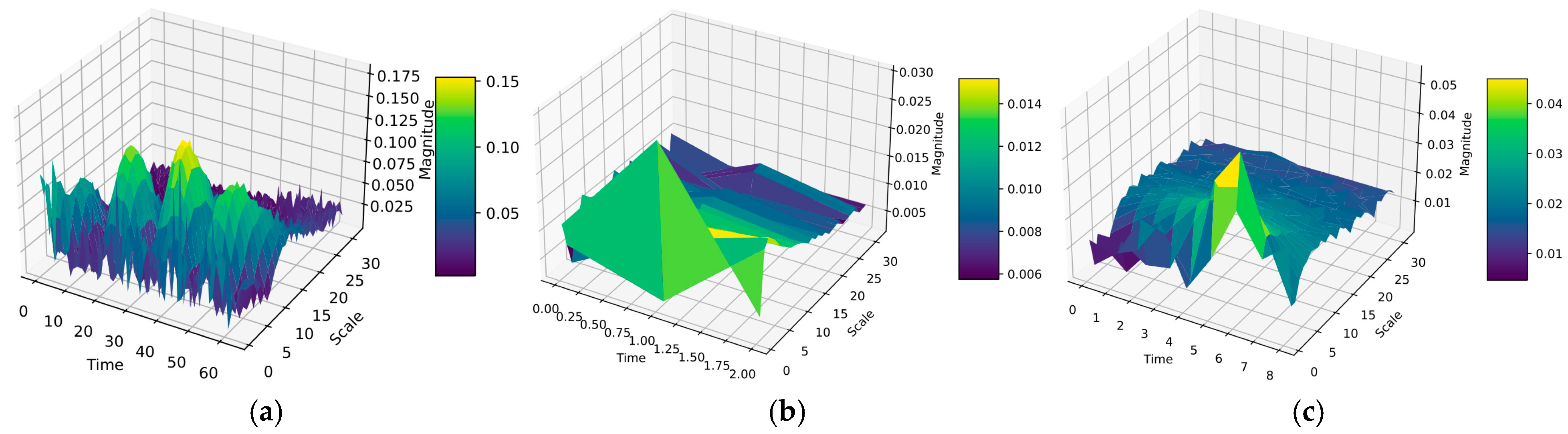
In deep learning models, understanding how each feature layer processes information of varying frequencies is crucial for optimizing the model. By visualizing the weights of convolutional layers, researchers can gain insights into how the model recognizes different fault patterns; this visualization helps to improve the interpretability of the model, which is highly valuable for the application of fault diagnosis technology. This paper employs the Short-Time Fourier Transform (STFT) to conduct a detailed analysis of the time–frequency properties of weights within each layer of the model. First, the weights of each convolutional kernel are averaged along the input channel dimension to obtain a one-dimensional weight sequence. Then, STFT is used to obtain the averaged one-dimensional weight sequence through a sliding window, where the STFT analysis calculates the amplitude and phase of each frequency component in each window, thereby transforming the one-dimensional weight sequence into a frequency domain representation. As the window slides along the time axis, STFT repeats this process at each position, gradually constructing a complete time–frequency matrix. Each column of this matrix represents the spectrum at a specific time point, and each row represents how a particular frequency changes over time. Finally, the results of this time–frequency analysis are visualized in the form of heatmaps, where different shades of color in the heatmap reflect the intensity of weight changes across different times and frequencies.

3. Experiments and Discussions

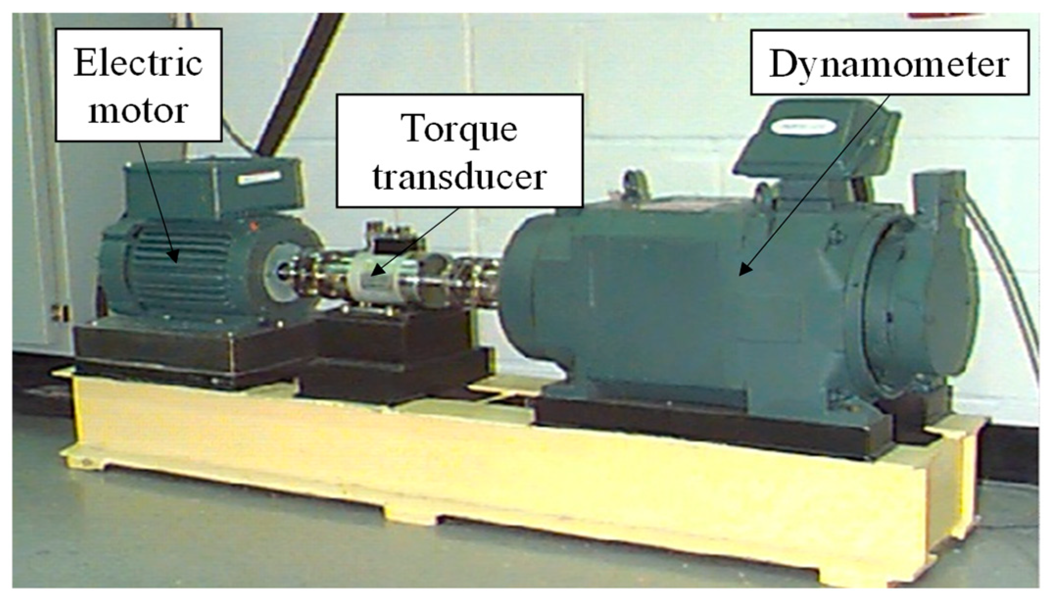
In this section, we provide an exhaustive description of the parameter configuration of the MCMBAN model. A series of fault diagnosis experiments are conducted on the bearing test platform of Case Western Reserve University (CWRU) as well as on our bearing test dataset https://github.com/haoppppp/MCMBAN.git (accessed on 31 July 2025).

3.1. Multi-Branch Cascade Attention Block (MBCAB)

Table 1. Hyperparameters of the proposed MCMBAN.

Type	Kernel Size	Stride	Channel
NMFB	32 × 1	4	16
Pooling	2 × 1	2	-
MBCAB	3 × 1/5 × 1/7 × 1/9 × 1	1	32
Pooling	2 × 1	2	-
MBCAB	3 × 1/5 × 1/7 × 1/9 × 1	1	64
Pooling	2 × 1	2	-
MBCAB	3 × 1/5 × 1/7 × 1/9 × 1	1	64
Pooling	2 × 1	2	-
GAP	-	-	-
Softmax	-	-	-

summarizes the detailed hyperparameter settings of the proposed MCMBAN model. The network architecture begins with a Noise Mask Filter Block (NMFB), which utilizes a 32 × 1 convolutional kernel with a stride of 4 and outputs 16 feature channels. This layer serves to initially capture coarse-grained features and suppress high-frequency noise through a wide receptive field. Following NMFB, a series of three Multi-Branch Convolution Blocks (MBCABs) are applied. Each MBCAB incorporates four parallel convolutional branches with kernel sizes of 3 × 1, 5 × 1, 7 × 1, and 9 × 1, designed to extract rich multi-scale features from the input. The first MBCAB outputs 32 channels, while the subsequent two each output 64 channels, enabling progressively deeper feature extraction. Between each MBCAB, a 2 × 1 max pooling layer with a stride of 2 is inserted to perform temporal downsampling, reducing the feature length by half at each stage while preserving critical information. After the final MBCAB, another pooling operation is applied before global aggregation. At the classification stage, a GAP layer is used to reduce each channel to a single value, with model outputs as the final class probabilities. Notably, the GAP and Softmax layers do not involve kernel or stride settings and are therefore denoted with dashes (“–”) in the table. These parameter choices are based on extensive empirical validation and are optimized to balance model capacity, noise robustness, and diagnostic precision.

3.2. Comparison Methods

By comparing MCMBAN with existing advanced techniques such as MCAMDN [22], RESCNN [23], MSDARN [24], MBSDCN [25], MA1DCNN [26], and GTFE-Net [27], its performance is evaluated, and the parameter details of comparison methods are shown in

Table 2. The details of the comparison methods.

Methods	Hyperparameter	Settings	Hyperparameter	Settings
MCAMDN	Channel Attention Spatial Attention MConvs DConvs Learning rate	1 1 4 4 0.002	Batch size Optimizer Loss function	32 SGD Cross-entropy loss
RESCNN	Res blocks Kernel size Max pooling Stride Learning rate	2 10 2 1 0.001	Batch size Optimizer Loss function	128 Adam Cross-entropy loss
MSDARN	Wide conv size Res blocks Maxpool layers Stride Learning rate	128 3 3 2 0.001	Dropout rate Batch size Optimizer Loss function	0.5 64 Adam Cross-entropy loss
MBSDCN	MBSDCLs Maxpool layers Conv size Stride Learning rate	2 2 3 2 0.001	Dropout rate Batch size Optimizer Loss function	0.2 32 Adam Cross-entropy loss
MA1DCNN	Wide conv size Conv size EAMs CAMs Stride Learning rate	32 16/9/6/3 5 5 1/2/4 0.0001	Pool Batch size Optimizer Loss function	GAP 196 Adam Cross-entropy loss
GTFE-Net	BGMs FLMs FCMs Stride Learning rate	1 5 1 2 0.001	Dropout rate Batch size Optimizer Loss function	0.2 32 Adam Cross-entropy loss

.

MCAMDN proposes a multi-scale selectable branch network structure, where each branch network contains convolution kernels with different sizes. The core idea is to use the attention mechanism to dynamically select effective branches and determine the contribution of each branch. However, the branches in MCAMDN operate independently and in parallel, lacking information interaction, whereas MCMBAN achieves cross-layer feature fusion through cascade attention.

RESCNN adopts a residual network architecture to alleviate the vanishing gradient problem by using residual connections. It also uses wide convolution layers to suppress high-frequency noise and enhance low-frequency feature extraction. However, its network structure is single-scaled and single-pathed, making it difficult to model multi-frequency features, pulse frequencies, etc. MCMBAN, on the other hand, covers the full frequency range of fault features through multi-branch multi-scale kernels.

MSDARN combines multi-scale convolution with a dynamic attention mechanism, using residual connections to fuse features from different scales and introducing adaptive weights to adjust inter-channel correlations. However, MSDARN fuses multi-scale features serially within a single branch, emphasizing the dynamism of scale feature fusion. In contrast, MCMBAN independently extracts features through parallel branches and then uses cascade attention for cross-layer interaction, emphasizing the diversity and interaction of scale features.

MBSDCN enhances channel expression through multi-branch input and a channel reconstruction attention mechanism, dividing input features into multiple branches. Each branch uses a fixed-size convolution kernel, and dynamic convolutions generate kernel weights. However, the fusion process primarily focuses on channels, lacking inter-layer structural interaction and independent denoising modules.

MA1DCNN embeds a multi-head attention mechanism into a 1D convolutional network, where each head independently computes feature correlations. The outputs from multiple heads are concatenated to enhance the model’s attention to fault impulse signals. However, MA1DCNN is a single-branch structure, and the attention mechanism only operates on the local layer. In contrast, MCMBAN is composed of a denoising module and feature cascading, with more efficient inter-layer collaboration.

GTFE-Net designs a frequency-domain filtering-based denoising method based on the periodicity and self-similarity characteristics of vibration signals. Additionally, it constructs a three-branch network structure to process the original vibration signal, denoised signal, and frequency spectrum signal. Compared to MCMBAN, GTFE-Net’s structure relies on external preprocessing modules, making its overall architecture more complex, and the feature fusion process is relatively static.

3.3. Experimental Environment and Noise Environment

In this study, all experiments are conducted using the TensorFlow 2.5 framework, with programming carried out in Python 3.7. The hardware required for the experiments included an RTX 3050 graphics card, an AMD 5600H processor, and 16GB RAM. The equipment was sourced from Lenovo, based in Hefei, China. We set 50 training cycles, 32 samples per batch. The learning rate is 0.001. The optimizer is the Adam optimizer, which reduces the fluctuations in training losses, and experimental results are evaluated by calculating the average accuracy over five iterations.

In actual industrial environments, the vibration signals collected are inevitably subjected to environmental noise interference. Environmental noise is commonly characterized as random, has a low bandwidth, and often has a non-stationary nature, with certain features resembling high-frequency interference. This paper discusses methods for filtering out such noise in complex environments. The signal-to-noise ratio (SNR) of the vibration signal is commonly used to quantify noise resistance. In this experiment, the noise interference is modeled as Gaussian white noise, and the SNR is calculated as follows:

$$\mathrm{SNR}=10{\log }_{10}{\displaystyle \frac{{‖\mathbf{X}‖}_2^2}{{‖\mathbf{X}-\Phi ‖}_2^2}}$$

(12)

where $\mathbf{X}$ is the original signal, $\Phi$ is the noise-corrupted signal, and ${‖·‖}_2^2$ is the square of the ${\mathcal{l}}_2\text{-}\mathrm{norm}$. In the process of adding noise, the power $P_x$ of each sample signal $x$ is first calculated:

$$P_x={\displaystyle \frac{1}{N}}{\displaystyle \sum _{i=1}^N{x}_i^2}$$

(13)

where $N$ represents the signal length. The target SNR values are set as 0 dB, −4 dB, and −6 dB, where a lower SNR corresponds to higher noise intensity. Based on the SNR values, the noise power $P_n$ is calculated as follows:

$$P_n=P_x·{10}^{-{\mathrm{SNR}}_{\mathrm{dB}}/10}$$

(14)

Subsequently, the noise standard deviation $\sigma =\sqrt{P_n}$ is calculated, and the noise is assumed to follow a Gaussian distribution $\epsilon \sim \mathbb{N}(0,{\sigma }^2)$.

Finally, the noise is added to the original signal to obtain the noisy signal $x_{\mathrm{noise}}$ as follows:

$$x_{\mathrm{noise}}=x+\epsilon$$

(15)

In summary, during the experiment, to simulate real-world conditions, noise is injected into the signals, and the noise levels are controlled to assess the model’s performance under various noise conditions. The goal is to ensure that the model maintains its robustness in the presence of noise and demonstrates practical applicability in real-world scenarios.

To ensure a fair comparison, all competing models were retrained under the same noise settings and consistent data splits. Specifically:

Noise settings: All models were trained and tested under identical noise conditions. This ensured that the comparison was not affected by variations in noise environments.

Data splits: A uniform data splitting strategy was applied. The training, validation, and testing sets remained the same across all models to guarantee consistency during evaluation.

The criteria for evaluating fault diagnosis (FD) results include four key metrics: accuracy, precision, recall, and F1 score. The calculation of these metrics is based on the following four types of samples: true positives (TP), true negatives (TN), false negatives (FN), and false positives (FP).

4. Experiments and Discussions

4.1. Case 1: Fault Diagnosis Experiment on CWRU Motor Bearings

4.1.1. Data Description

The bearing fault dataset constructed by the CWRU Bearing Data Center systematically encompasses multiple fault modes and their varying degrees of severity. As shown in

Table 3. Description of the CWRU rolling bearing dataset.

Class Label	Sample	Fault Size (in)	Fault Location
0	600	0	Normal
1	600	0.007	Inner race
2	600	0.014	Inner race
3	600	0.021	Inner race
4	600	0.007	Outer race
5	600	0.014	Outer race
6	600	0.021	Outer race
7	600	0.007	Ball
8	600	0.014	Ball
9	600	0.021	Ball

, the operational states of bearings are classified into 10 distinct categories, including normal conditions and three major fault types: outer race faults, inner race faults, and rolling element faults. Each fault type is further subdivided into three severity levels based on defect sizes ranging from 0.007 in to 0.021 in. During data acquisition, a window length of 1024 sampling points was adopted, and the sliding step of 200 sampling points was set to enhance data utilization. For the drive-end vibration signals, the dataset was collected at a sampling frequency of 12 kHz. Through the sliding window processing, a total of 6000 samples were generated. These samples were evenly divided into six subsets, with four subsets allocated for model training and the remaining two designated for validation and testing tasks, respectively. As illustrated in Figure 4, the hierarchical structure of the dataset clearly demonstrates the classification of different fault types and their corresponding severity levels.

4.1.2. Experimental Analysis of Motor Bearing Fault Diagnosis in Noisy Environment

The performance degradation of various fault diagnosis (FD) strategies under increasing noise interference is demonstrated in

Table 4. The diagnosis accuracy of methods on CWRU motor bearing fault in different noisy environments.

SNR	MCAMDN	RESCNN	MSDARN	MBSDCN	MA1DCNN	GTFE-Net	MCMBAN
0 dB	85.40%	88.98%	98.17%	98.68%	98.28%	99.17%	99.70%
−4 dB	86.80%	82.89%	92.91%	94.23%	93.80%	97.91%	98.75%
−6 dB	82.70%	76.81%	88.41%	90.15%	90.06%	95.41%	96.15%
Average	84.97%	82.89%	93.16%	94.35%	94.05%	97.50%	98.20%

. The signal-to-noise ratio (SNR), measured in decibels (dB), serves as the key indicator of noise intensity, where lower negative values correspond to stronger noise contamination. Analysis reveals a consistent performance decline across most methods as environmental noise escalates from 0 dB to −6 dB, attributable to the noise-induced masking effect on subtle fault signatures. Notably, the experimental data confirm that enhanced noise levels significantly compromise the models’ capability to discern critical fault characteristics. However, the proposed MCMBAN model consistently exhibits superior performance across all tested noise levels, demonstrating its excellent noise immunity. Specifically, MCMBAN achieves an average accuracy of 98.20%, which is ranked first among all evaluated methods, indicating its ability to maintain consistent performance across a variety of noise backgrounds. Observing the accuracy changes from 0 dB to −6 dB, from 99.70% to 96.15%, MCMBAN shows the smallest decline in performance, further proving its superior robustness. Overall, thanks to the efficient noise reduction capability of NMFB and the complex multi-scale learning mechanism of MBCAB introduced in Section 2, the MCMBAN demonstrates outstanding stability and high accuracy when facing challenges of varying noise levels.

4.1.3. Experimental Analysis of Diagnosing Different Types of Faults in Motor Bearings

Fault diagnosis experiments were conducted under three noise conditions with signal-to-noise ratios (SNRs) of 0 dB, −4 dB, and −6 dB, respectively. The diagnostic results for each fault type under these conditions are shown in Figure 5. According to the labeling scheme, label 0 represents the normal condition, labels 1–3 inner race faults, labels 4–6 outer race faults, and labels 7–9 rolling element faults. Larger label values indicate more severe damage. Based on the model’s diagnostic performance across different fault locations and severities, as well as the impact of noise on diagnostic accuracy, the following detailed analysis is provided:

Under 0 dB noise interference, the model achieved 100% accuracy in identifying the normal condition, clearly distinguishing it from all fault states. The diagnosis of inner race faults was almost error-free, indicating that the model effectively captures the periodic impact characteristics associated with inner race damage and can robustly identify varying levels of severity. The model also demonstrated high precision in identifying outer race and rolling element faults, with only a few misclassified samples. These results suggest that under low-noise conditions, the model can clearly discriminate between the impulse characteristics of different fault locations.

Under −4 dB noise interference, a slight overall performance decline was observed. The accuracy of inner race fault diagnosis remained relatively stable, while that of outer race faults decreased moderately. Rolling element fault accuracy exhibited a more significant drop, indicating that under moderate noise, the outer race fault features become less stable and increasingly overlapped with those of rolling elements in the frequency domain. The high-frequency transient spikes of rolling element faults, typically of low amplitude, were attenuated by the noise, leading to confusion with other categories. Thus, at −4 dB, the decline in diagnostic accuracy is mainly attributed to performance degradation in the detection of outer race and rolling element faults, validating the vulnerability of weak periodic and high-frequency transient features to moderate noise interference.

Under −6 dB noise interference, a notable deterioration in diagnostic performance was observed. The accuracy for identifying the normal condition remained largely unaffected. Inner race fault diagnosis remained relatively stable, although label 1 showed a slight decline, while label 3 maintained high accuracy. This suggests that inner race faults with strong periodicity and large-amplitude impacts exhibit strong robustness to noise. However, the diagnosis of outer race faults deteriorated significantly, with a notable increase in misclassification for label 5 and some confusion observed for label 6. This indicates that the semi-periodic impulses of outer race faults become severely distorted under strong noise, making accurate detection difficult. Rolling element fault diagnosis performance declined sharply, especially for label 8, which showed severe misclassification. This is primarily because the transient spikes associated with rolling element faults have inherently low amplitudes and, when strongly masked by noise, their features become indistinct, limiting the effectiveness of the model’s high-frequency detection capability.

4.2. Case 2: Fault Diagnosis Experiment on the Compound Bearing Fault Dataset

4.2.1. Data Description

The research on both single and complex bearing fault types is conducted using the Mechanical Fault Simulator (MFS) produced by Spectrum Quest Incorporated, which includes a drive motor end, accelerometers, and a signal acquisition device, as detailed in Figure 6. The simulator connects the motor to the drive system via a flexible coupling, and it uses laser technology to successfully replicate faults in the ball, inner ring, outer ring, and combined inner and outer rings. Vibration signals are collected at a frequency of 15.6 kHz; the compound fault data are shown in

Table 5. Description of the MFS compound fault dataset.

Fault Location	Samples	Fault Size (mil)	Class Label
Ball	200	6	0
Inner race	200	24	1
Outer race	200	6	2
Compound (Inner race and Outer race)	200	Inner 6 and Outer 9	3

. Additionally, the bearings operate at a speed of 1130 rpm. In order to handle the limitations of sensor data collection, we set a window length of 1024 points for data collection, with each window containing 200 fault samples, resulting in a total of 800 data samples. And, 500 samples were allocated for training the model, 150 for validation, and the remaining 150 for the final test phase.

4.2.2. Experimental Analysis of Compound Bearing Fault Dataset in Noisy Environments

In practical applications, bearing complex faults occurs frequently, and their diagnosis is more challenging than that of single faults. In order to assess the real-world feasibility of the results of this study, three distinct noise levels are established for the complex fault data.

Table 6. The diagnosis accuracy of methods on the compound fault in different noisy environments.

SNR	MCAMDN	RESCNN	MSDARN	MBSDCN	MA1DCNN	GTFE-Net	MCMBAN
0 dB	92.56%	85.98%	90.55%	95.66%	92.35%	93.20%	97.80%
−4 dB	86.88%	78.92%	83.92%	90.10%	85.74%	90.15%	93.45%
−6 dB	84.60%	75.48%	80.35%	87.60%	81.30%	88.62%	90.12%
Average	88.01%	80.13%	84.94%	91.12%	86.46%	90.66%	93.79%

shows the performance of various fault diagnosis (FD) methods under different noise environments. The proposed MCMBAN demonstrates a significant advantage under various noise conditions, achieving an accuracy of 97.80% at a 0 dB noise level and maintaining 90.12% even in a high noise environment of −6 dB. These results validate MCMBAN’s robust capacity to resist noise interference and handle complex fault conditions. Furthermore, the MCMBAN has an average accuracy of 93.79%, which is significantly higher than other comparing methods, highlighting its superior performance in diagnosing complex bearing faults. The MCMBAN demonstrates remarkable accuracy even with a limited sample size of only 500 training samples. This can be particularly significant in scenarios where sample acquisition costs are considerable.

4.2.3. Experimental Analysis of Different Types of Composite FDS in a Noisy Environment

This section presents the diagnostic results of different bearing fault types under three levels of noise, as shown in Figure 7. Under the 0 dB noise condition, the recognition accuracy for both the rolling element and inner race faults exceeds 99%, indicating that the model can clearly capture the characteristic features of these fault types. A small number of outer race faults are misclassified as inner race or compound faults. The compound fault recognition accuracy reaches 99.3%, demonstrating that the model can effectively distinguish the superimposed impact features of both inner and outer race faults.

When the noise level increases to −4 dB, the diagnostic accuracy for rolling element and inner race faults remains largely unaffected, reflecting the model’s strong noise robustness. However, a small number of outer race fault samples are misclassified as inner race or compound faults, indicating that the low-amplitude features of outer race faults begin to degrade under moderate noise. In addition, a considerable number of compound faults are misclassified as inner race faults, suggesting that the outer race features in compound faults are significantly masked by medium-intensity noise.

Under the −6 dB high-noise condition, the recognition accuracy for rolling element and inner race faults remains relatively high. However, the diagnostic accuracy for outer race faults drops substantially, indicating that the model’s ability to capture the impact features of outer race faults becomes notably limited. Some compound fault samples are also misclassified as inner race faults. These observations imply that the primary influence of noise lies in the attenuation or blurring of low-amplitude and high-frequency features, particularly affecting the diagnosis of outer race and compound faults, while having a relatively minor impact on rolling element and inner race faults. Future improvements may focus on enhancing the model’s capacity to identify low-amplitude and high-frequency components under strong noise environments.

4.3. Analysis of Ablation Experiment

4.3.1. Contributions of NMFB and MBCAB

To evaluate the individual and combined contributions of the proposed NMFB and MBCAB modules, we conducted a set of ablation experiments, as summarized in

Table 7. Results of ablation experiment.

Method	NMFB	MBCAB	Accuracy
1	-	-	79.25%
2	-	√	88.36%
3	√	-	93.90%
4	√	√	98.20%

. Four configurations were tested: Method 1 represents the baseline model without NMFB or MBCAB components, achieving an accuracy of 79.25%. This relatively low performance highlights the limitations of the base architecture in extracting robust and discriminative features under noisy conditions. Method 2 incorporates only the MBCAB module. With the ability to extract multi-scale features through parallel convolutions of varying kernel sizes, the model performance significantly improves to 88.36%. This demonstrates the importance of capturing diverse temporal patterns in vibration signals. Method 3 includes only NMFB. By suppressing high-frequency noise and enhancing fault-relevant patterns through wide convolutions and attention-based filtering, this variant achieves an accuracy of 93.90%, indicating that noise reduction plays a critical role in improving diagnostic reliability. Method 4, the full model combining both NMFB and MBCAB, achieves the highest accuracy of 98.20%. This result validates the complementary strengths of both modules: NMFB enhances noise robustness, while MBCAB enables effective multi-scale feature extraction. Their integration leads to a synergistic improvement in diagnostic performance. These results confirm that both NMFB and MBCAB are essential components of the proposed architecture, each contributing substantially to its overall effectiveness in fault detection tasks.

4.3.2. Complexity Analysis of the Model

To evaluate the impact of NMFB and MBCAB modules on the overall efficiency of the model, this paper provides additional results on the training time and computational complexity under different method configurations, as shown in

Table 8. Model training time and computational complexity under different configurations.

Method	NMFB	MBCAB	Training Time	Parameters
1	-	-	104 s	0.202 M
2	-	√	191 s	4.244 M
3	√	-	121 s	0.206 M
4	√	√	244 s	4.249 M

. The parameter count is measured in millions (M), representing the total number of weights and biases in the model, while the training time is measured in seconds (s). Method 1 is the baseline model, which does not include NMFB and MBCAB modules. It has the lowest parameter count of 0.202 M and the shortest training time of 104 s. However, its performance is limited, making it ineffective in handling noise interference and multi-scale feature extraction. Method 2 introduces the MBCAB module to the baseline model, significantly increasing the parameter count to 4.244 M and the training time to 191 s. However, the model’s feature extraction capability is significantly enhanced, validating the effectiveness of MBCAB in multi-scale feature learning. Method 3 replaces the MBCAB module with a conventional convolutional structure and introduces NMFB. The parameter count and training time are 0.206 M and 121 s, respectively. Compared to Method 1, there is a slight increase, but the noise resistance performance has been significantly improved, indicating that NMFB has good noise resistance and adds only a small number of parameters. Method 4 is the complete MCMBAN model, incorporating both the NMFB and MBCAB modules. It has the highest training time of 244 s and the highest parameter count of 4.249 M, but it performs the best in terms of classification accuracy, robustness, and other metrics. In summary, the analysis of the results regarding the impact of different modules on model efficiency shows that NMFB significantly enhances the model’s noise resistance while maintaining minimal computational overhead, and the MBCAB module plays a crucial role in enhancing multi-scale feature modeling. Although the introduction of both modules adds some resource consumption, the overall training time remains under 5 min, meeting the requirements for fast deployment and iteration in industrial scenarios. Moreover, despite the increase in the parameter count of the MCMBAN model to 4.249 M, it remains lightweight compared to mainstream deep learning models and has good potential for edge deployment. Furthermore, the NMFB and MBCAB modules are clearly structured and function independently, allowing for flexible use according to practical needs, making them well-suited for balancing practicality and computational efficiency in industrial applications.

4.3.3. Impact of Mask Threshold on Model Performance

From the ablation experiment results in

Table 9. Results of NMFB’s mask threshold on model performance.

Top k	k = 0.2	k = 0.4	k = 0.8
Accuracy	92.25%	93.81%	96.15%

, it is evident that NMFB mask threshold has a significant impact on model performance. As the threshold k increases, the model’s accuracy gradually improves, reaching 92.25%, 93.81%, and 96.15%. When k = 0.2, the model retains more low-correlation features, resulting in a lower accuracy. This suggests that retaining too many low-correlation features may introduce noise interference, affecting the model’s diagnostic ability. When increased to 0.4, the model begins to ignore some low-correlation features and retains more representative ones, leading to a significant improvement in accuracy to 93.81%. This indicates that moderately increasing the threshold helps reduce noise interference and optimize feature selection. Finally, when k = 0.8, the model’s accuracy reaches 96.15%, demonstrating that a higher threshold effectively focuses on the most representative features, significantly enhancing model performance. This trend suggests that increasing the threshold helps the model reduce redundant information and noise interference, thereby improving accuracy. However, choosing the appropriate threshold remains crucial, as excessively high thresholds may discard some valuable weakly correlated features. Therefore, appropriately adjusting the mask threshold not only ensures high performance but also contributes to optimizing the model’s robustness and stability.

Theoretical derivation of threshold selection in top-k: In NMFB, a wide convolution layer is first introduced to enhance low-frequency structures and suppress high-frequency noise. However, a potential drawback of this low-pass property is that it may excessively attenuate high-frequency impact signals related to faults, resulting in the loss of critical diagnostic information. To solve this issue, NMFB further incorporates a self-attention mechanism based on Top-k masking, which dynamically selects relevant features to compensate for the high-frequency information loss caused by wide convolution.

From a mathematical perspective, the Top-k mask effectively controls the sparsity and rank of the attention matrix. The choice of the Top-k value directly influences whether the matrix rank can recover sufficient feature diversity. When k is relatively small (e.g., 0.2 or 0.4), the number of non-zero elements retained in the attention matrix is limited, resulting in a sparser matrix with a lower rank. In this case, high-frequency impulses suppressed by the wide convolution are further filtered out, retaining only strong correlations among low-frequency features, which leads to the loss of many fault-related details. In contrast, when k is relatively large (e.g., 0.8), the attention matrix becomes denser and its rank increases significantly. The matrix not only preserves the low-frequency periodic features from the wide convolution output but also retains detailed high-frequency impact information, thereby achieving joint feature modeling of low-frequency trends and high-frequency pulses.

4.3.4. Analysis of the Model Generalization Performance

In intelligent fault diagnosis tasks, the model generalization capability is a crucial criterion for evaluating its practicality. To assess the model’s generalization performance under different operating conditions, this study constructs six cross-load testing tasks based on three load conditions (1 hp, 2 hp, and 3 hp) from the CWRU dataset, covering all combinations where the training and testing loads are inconsistent (e.g., 1→2 denotes training on 1 hp and testing on 2 hp). The experimental results of each model across the six variable-load tasks are presented in

Table 10. Test results for the generalization performance of different models under variable loads.

Variable Load	MCAMDN	RESCNN	MSDARN	MBSDCN	MA1DCNN	GTFE-Net	MCMBAN
1→2	98.20%	92.25%	98.68%	92.05%	97.79%	94.67%	98.95%
1→3	92.58%	88.79%	97.10%	89.85%	94.55%	91.10%	96.40%
2→1	95.15%	90.68%	97.21%	89.34%	97.90%	91.89%	97.66%
2→3	97.20%	94.31%	98.34%	91.23%	98.35%	94.65%	98.40%
3→1	94.10%	90.05%	94.11%	88.47%	90.71%	89.39%	93.68%
3→2	93.35%	93.60%	95.89%	89.35%	95.89%	91.20%	96.91%
Average	95.18%	91.61%	96.89%	90.05%	95.87%	92.15%	97.00%

. The proposed MCMBAN achieves the highest accuracy in three tasks and demonstrates robust performance in the remaining tasks, ultimately attaining an average accuracy of 97.00%. Although MCMBAN was not explicitly optimized for cross-condition adaptability, its architectural emphasis on multi-scale feature fusion and noise robustness enables it to exhibit strong generalization. This enables the model to effectively handle signal mode changes caused by load variations, confirming the model’s adaptability to diverse operating conditions in actual industrial environments.

4.3.5. The Impact of the Sample Size on the Model

To investigate the impact of sample size on the performance of the proposed model, comparative experiments were conducted on both the CWRU dataset and the MFS compound fault dataset. The ratio of training, validation, and test sets was kept constant, with the results as shown in

Table 11. The impact of the sample size on the model.

Datasets	Sample Size	Accuracy
CWRU dataset	3000	90.40%
	6000	96.15%
	9000	97.28%
MFS compound fault dataset	400	86.71%
	800	90.12%
	1200	92.36%

, on the CWRU dataset; when the number of samples increased from 3000 to 6000, the model accuracy improved significantly from 90.40% to 96.15%. This indicates that a small number of samples may lead to insufficient feature learning. When the sample size further increased to 9000, the accuracy reached 97.28%. Although the improvement was smaller, it still showed performance gains. Considering the trade-off between training cost and accuracy, 6000 samples were used as the standard setting in our main experiments to balance performance and efficiency.

On the MFS compound fault dataset, the accuracy increased from 86.71% to 90.12% and 92.36% as the sample size increased from 400 to 800 and 1200, respectively. This shows a consistent performance improvement trend. These results demonstrate that the proposed model maintains good scalability and robustness under different data sizes. Overall, the experiments confirm that the model adapts well to varying sample scales and achieves high accuracy even with small or medium-sized datasets.

4.4. Feature Interpretability Analysis of the Model

By visualizing the weights of each feature layer in the model, we can analyze the contribution of each layer to the final fault diagnosis decision and improve the feature interpretability of the model. Figure 8a–c show the weights of the input convolutional layers, the weights of the NMFB layer, and the weights of the MBCAB layer, respectively. It can be seen that the input convolutional layer directly processes the raw vibration signal. The weights of this layer show some leveling off, indicating that the layer is extracting generic features and not focusing on extreme or high-frequency variations. The weights of the NMFB layer show more dynamic variations with larger amplitude variations, indicating that it is processing higher-frequency signals or more complex features. The NMFB layer performs feature extraction through the wide convolution and multi-attention mechanism. The attention mechanism allows the network to focus on important information and ignore irrelevant signals, thus improving the network’s discriminative ability. The weights of the MBCAB layer focus on shorter time scale changes, indicating that it concentrates on capturing fast, instantaneous feature changes. The MBCAB layer analyzes the periodic impulsive features of the signals by the multi-scale convolution and cascading attention mechanism. This design allows the network to capture and emphasize highly correlated impulse signals caused by bearing failures. In summary, the functions and contributions of each layer are analyzed by CWT time–frequency transform, which makes the proposed model more transparent and acceptable in practical applications.

In Figure 8, the correlations between weight variations and specific fault types are analyzed as follows:

In the visualization of the input convolutional layer (Figure 8a), three approximately equidistant energy ridges appear along the time axis, with ridge peaks concentrated in the mid-scale range. Since inner race defects occur at a fixed contact angle between the rolling element and the inner raceway, a high-amplitude impact is excited once per shaft rotation, producing a stable characteristic frequency. Therefore, the periodicity and harmonic alignment of the energy ridges indicate that the harmonic structure in the learned weights corresponds to the stable excitations caused by inner race defects, suggesting that the input convolutional layer is learning the consistent impact features induced by such defects.

In NMFB layer weight visualization (Figure 8b), the high-frequency components exhibit overall suppression, while the low-frequency components remain gradually attenuated. This pattern indicates that the network imposes high resistance to high-frequency components while allowing low resistance to mid- and low-frequency ones. As environmental noise typically resides in the high-frequency broadband region and the primary impact information of bearing faults is located in the mid- and low-frequency bands, the high-frequency suppression observed in the NMFB layer demonstrates the network’s role in attenuating noise components and preserving clean spectral regions for subsequent feature extraction.

The MBCAB layer weight visualization (Figure 8c) displays isolated and sharp peaks, which are temporally narrow and vertically locked to the small-scale high-frequency band. These sharp peaks imply that the convolutional kernels have been trained as narrowband transient detectors, assigning high weights to short-duration high-frequency impulses. In the cases of rolling element and compound faults, random collisions generate concentrated bursts of high-frequency transient energy, matching the time–frequency patterns of these peaks. This indicates that the network is capturing such transient spikes to identify rolling element and compound faults effectively.

In summary, the input convolutional layer lays the foundation for detecting stable periodic impacts caused by inner race faults; the NMFB layer suppresses broadband noise, ensuring that impact patterns are not obscured; and the MBCAB layer captures random high-frequency spikes associated with rolling element and compound faults. Together, these layers collaboratively extract features specific to inner race, outer race, and rolling element faults, endowing the model with a clear and physically interpretable diagnostic mechanism.

5. Conclusions

This paper proposes the MCMBAN model, a novel technique designed to solve the problem of high noise impact and highly similar fault types encountered in mechanical fault diagnosis. This network utilizes a combination of a Noise Mask Filter Block (NMFB) and a Multi-Branch Cascade Attention Block (MBCAB) to significantly enhance the capability to recognize fault signal features and suppress noise. Extensive experiments demonstrate that the MCMBAN effectively improves the accuracy of fault diagnosis, outperforming six existing mainstream methods, both on the standard dataset provided by CWRU and our complex bearing dataset. In addition, a detailed analysis of the feature learning process of MCMBAN has revealed how the network improves fault type recognition and isolation through various levels of feature layers. This analysis not only proves the effectiveness of the proposed method but also enhances the feature interpretability of the network model. Future work will focus on expanding the theoretical foundation and practical application areas of MCMBAN, aiming to further improve its applicability and explainability in mechanical fault diagnosis.