Abstract
The ship waterjet propulsion system is a crucial power unit for high-performance vessels, and the operational state of its core component, the waterjet pump, is directly related to navigation safety and mission reliability. To enhance the intelligence and accuracy of pump fault diagnosis, this paper proposes a novel diagnostic framework that integrates a supervised autoencoder (SAE) with a large language model (LLM). This framework first employs an SAE to perform task-oriented feature learning on raw vibration signals collected from the pump’s guide vane casing. By jointly optimizing reconstruction and classification losses, the SAE extracts deep features that both represent the original signal information and exhibit high discriminability for different fault classes. Subsequently, the extracted feature vectors are converted into text sequences and fed into an LLM. Leveraging the powerful sequential information processing and generalization capabilities of LLM, end-to-end fault classification is achieved through parameter-efficient fine-tuning. This approach aims to avoid the traditional dependence on manually extracted time-domain and frequency-domain features, instead guiding the feature extraction process via supervised learning to make it more task-specific. To validate the effectiveness of the proposed method, we compare it with a baseline approach that uses manually extracted features. In two experimental scenarios, direct diagnosis with full data and transfer diagnosis under limited-data, cross-condition settings, the proposed method significantly outperforms the baseline in diagnostic accuracy. It demonstrates excellent performance in automated feature extraction, diagnostic precision, and small-sample data adaptability, offering new insights for the application of large-model techniques in critical equipment health management.
1. Introduction
Waterjet propulsion systems are advanced marine propulsion devices known for their high efficiency, low noise, and superior maneuverability [1,2]. They are widely used in high-speed passenger ships, coast guard vessels, and modern warships. The waterjet pump, as the core power component of this system, has a complex internal structure and operates under severe conditions of high rotational speed and high pressure. Key components like the impeller and guide vane are prone to various faults such as cavitation, wear, and cracking [3]. If such faults are not detected and diagnosed in a timely manner, they can degrade vessel performance or even cause catastrophic accidents, posing serious threats to navigation safety. Therefore, developing accurate and intelligent fault diagnosis techniques for waterjet pumps is of critical theoretical and practical importance for ensuring the reliability and availability of ship equipment.
Fault diagnosis based on vibration signal analysis is currently one of the primary methods for monitoring the health of rotating machinery [4]. By installing accelerometers at critical locations of the pump (e.g., the guide vane casing), vibration signals can be collected to effectively capture information about the equipment’s operating state. Traditional diagnostic methods typically rely on signal processing techniques such as Fourier transforms or wavelet analysis, combined with expert knowledge, to manually design and extract a series of time-domain and frequency-domain features that characterize fault information [5]. However, these approaches have clear limitations: first, the feature extraction process is highly dependent on domain expertise and diagnostic experience, making it subjective, time-consuming, and labor-intensive; second, in practical applications the vessel’s operating conditions often vary (e.g., changes in speed or load), leading to complex and variable pump operating states. Features that are manually designed may have limited cross-condition adaptability and generalization capability in such scenarios [6].
In recent years, data-driven fault diagnosis methods based on artificial intelligence, particularly deep learning, have achieved remarkable success [7,8]. Models like convolutional neural networks (CNNs) and recurrent neural networks (RNNs) can automatically learn fault features from raw signals, overcoming to some extent the drawbacks of manual feature extraction [9,10]. Despite this, traditional deep learning models still face challenges, especially in industrial scenarios with limited few data or cross-condition variations. Early fault samples are often scarce, and data distributions can differ between different machines or production batches, leading to dramatic performance drops and greatly limiting the effectiveness and broad applicability of existing diagnostic methods [11,12].
Large language models (LLMs) represent a revolutionary breakthrough in AI, and their unprecedented generalization, reasoning, and sequence-understanding capabilities are reshaping many research fields [13,14,15]. Recent studies have shown that LLMs exhibit great potential in time series analysis tasks, offering a new perspective on addressing the aforementioned challenges in fault diagnosis. By converting sensor-collected signals or their features into text formats that LLMs can process, and by combining parameter-efficient fine-tuning (PEFT) techniques such as LoRA, LLMs can be adapted to diagnostic tasks, thereby leveraging their strong capabilities in limited few data fault diagnosis and cross-condition generalization.
However, the application of LLMs to fault diagnosis is still in its early stages. One representative approach [16] is to use an LLM by converting manually extracted time-domain and frequency-domain features into text sequences for fine-tuning. While this method takes advantage of the LLM’s generalization ability, it does not solve the fundamental problem of relying on manually crafted features. The quality of the input representations fundamentally limits the model’s performance; suboptimal manual features may hinder the LLM from fully realizing its potential.
To overcome this limitation, this paper proposes a novel waterjet pump fault diagnosis framework that combines a supervised autoencoder (SAE) with a large language model (LLM). The framework aims to integrate task-oriented automated feature learning with the powerful generalization ability of LLMs. The main contributions of this paper are as follows:
- Firstly, we abandoned the traditional LLM fault diagnosis framework of manually extracting time–frequency domain features. Instead, we employ a supervised autoencoder (SAE) to directly learn deep features from raw vibration signals that are oriented toward the fault classification task. This achieves automated feature extraction while ensuring that the features optimally discriminate between different fault types.
- Secondly, a deep, integrated, intelligent diagnostic framework was constructed, which combines the high-quality features learned by the SAE with the powerful generalization and reasoning capabilities of an LLM. By using parameter-efficient fine-tuning techniques, we construct an end-to-end, high-precision diagnostic model.
- Finally, we comprehensively validated the superiority of the proposed framework by conducting comprehensive experiments under two key scenarios: direct diagnosis with full data and transfer diagnosis under limited-data conditions. The results showed that compared to the baseline method using manually extracted time–frequency features, our framework significantly improves diagnostic accuracy, generalization, and data efficiency.
The remainder of this paper is organized as follows: Section 2 reviews related work in fault diagnosis, including traditional methods, deep learning approaches, and the current applications of large language models. Section 3 describes the baseline LLM fault diagnosis framework and the proposed SAE-LLM fault diagnosis framework in detail. Section 4 presents the experimental setup and analysis of the results. Finally, Section 5 summarizes the paper and discusses future work.
2. Related Work
This section reviews research progress in three aspects: (1) data-driven fault diagnosis techniques, covering both traditional and deep learning methods; (2) text sequence format input in fault diagnosis based on LLM; (3) the application of LLM fine-tuning technology in fault diagnosis and health management.
2.1. Based on Data-Driven Fault Diagnosis Techniques
Fault diagnosis is a critical process to ensure the reliable operation of machinery, and vibration signal analysis is one of the most effective approaches. Early research focused on signal processing techniques. Fourier transforms were used to analyze the frequency spectrum of signals, or wavelet transforms were employed for time–frequency analysis [17] to identify characteristic frequencies associated with specific faults (e.g., bearing inner or outer race faults). These methods are theoretically mature but highly dependent on prior knowledge, and they perform poorly when dealing with complex, non-stationary signals.
With the advancement of AI, data-driven fault diagnosis methods, especially deep learning, have attracted widespread attention [18]. Lei et al. [4] highlight this trend in their review. Researchers have successfully used CNNs to classify two-dimensional representations of vibration signals (such as spectrograms or scalograms) [9] and have applied RNNs and their variants (e.g., long short-term memory networks, LSTMs) to directly model temporal dependencies in raw time series data [10]. These deep learning models can automatically learn features, reducing reliance on manual feature design. However, they also have limitations. They typically require large amounts of precisely labeled training data, and their generalization ability drops significantly under changing operating conditions or different machines [19,20]. To address this issue, researchers have explored techniques like transfer learning and domain adaptation to improve model robustness when facing data scarcity or domain shifts [21,22,23]. Despite these advances, achieving high accuracy in few-shot or zero-shot scenarios remains a major challenge.
2.2. Text Sequence Format Input in LLM-Based Fault Diagnosis
LLMs were originally designed for natural language processing (NLP) tasks, but their powerful learning and reasoning capabilities have rapidly expanded their applications to fields such as computer vision, healthcare, finance, and more. Applying LLMs technology to prognostics and health management (PHM) is an emerging and promising research direction [24,25]. LLMs’ strong generalization ability and in-context learning capabilities offer novel perspectives for solving critical challenges in the fault diagnosis field, such as low diagnostic accuracy under limited-data scenarios (few-shot fault diagnosis) and weak generalization ability under cross-condition transfer diagnosis. Nevertheless, a key challenge in applying LLMs to fault diagnosis lies in converting raw non-textual signals (e.g., vibration data) into textual sequences suitable for LLM processing.
Tao et al. [16] provide a typical example; they manually extracted 12 time-domain features (such as mean, standard deviation, kurtosis, crest factor, etc.) that describe the overall statistical characteristics of the signal and 12 frequency-domain features (such as frequency mean, frequency centroid, etc.) that reveal the periodic components of the signal as input to an LLM. The advantage of this approach is that the features have clear physical meanings, but the drawbacks are that the process is cumbersome and the extracted features may not be optimal. Particularly under complex operating conditions, their generalization ability may be limited. To overcome the limitations of manual features, supervised automated feature learning methods have been developed. For instance, the supervised autoencoder leverages label information during training to learn latent features that are both compact and highly discriminative for fault categories [26,27,28]. Crucially, the effectiveness of any subsequent conversion of these learned features into textual sequences for LLM processing hinges on their quality and relevance to the diagnostic task.
In current research on fault diagnosis based on LLM, the formatting design of text sequence inputs has formed a systematic paradigm [16]. The mainstream method generally adopts a structured triplet framework, which is the collaborative construction of Instruction, Input, and Output. The Instruction specifies the diagnostic objective (such as “identifying bearing fault types based on vibration signals”) and provides task semantic guidance for the model; Input converts the original signal into processable text through manual feature description or automated feature text conversion; Output defines standardized output formats (such as fault category labels or probability distributions). This structured input significantly improves the task adaptability of LLM.
2.3. LLM Fine-Tuning Technology in Fault Diagnosis
The core advantages of LLMs lie in their strong generalization and contextual learning abilities. By pre-training on massive datasets, LLMs can capture a broad range of knowledge and patterns, and through fine-tuning on specific downstream tasks, they can quickly adapt to new domains [29,30].
Traditional full-parameter fine-tuning updates all the weights of the LLM, which achieves optimal performance but at a very high computational cost [31]. To mitigate this, several parameter-efficient fine-tuning methods have been proposed. Li & Liang [32] introduced prefix tuning, a lightweight approach that optimizes continuous prefix vectors without modifying the main model parameters, thereby saving significant storage and tuning costs. Houlsby et al. [33] proposed adapter tuning, which inserts small neural modules (adapters) into each layer of the pre-trained network; during fine-tuning, only these adapters are trained while the original model parameters are kept fixed. Lester et al. [34] proposed prompt tuning, which introduces learnable continuous embeddings (prompts) into the model inputs; these prompts are updated during training to guide the model to produce outputs more suitable for the task. Hu et al. [35] proposed LoRA (Low-Rank Adaptation), which freezes the pre-trained model weights and injects trainable low-rank decomposition matrices into each layer, greatly reducing the number of trainable parameters and significantly lowering computational and memory requirements.
Fine-tuning the pre-trained LLMs and applying it to the field of fault diagnosis is a promising research direction in recent years. Since fault diagnosis tasks can essentially be viewed as time series classification problems, which aligns well with LLMs’ strengths in handling sequential data. Tao et al. [16] manually extracted features from raw bearing vibration signals, converted them to text sequence format inputs for LLM, and fine-tuned the LLM with these text sequences under supervised instruction. To make this process computationally feasible for large models, they used LoRA to freeze the model’s weights and inject low-rank matrices, substantially reducing the number of trainable parameters. This method cleverly transforms the diagnosis problem into a text classification task, demonstrating the potential of LLMs in diagnostic applications. However, as mentioned earlier, it remains limited by the quality of the manually extracted features.
2.4. Gap Analysis
In summary, existing research has advanced fault diagnosis techniques from multiple perspectives. However, the following research gaps remain:
- Suboptimal LLM inputs: Current LLM-based diagnosis methods either rely on suboptimal, time-consuming manual extraction of time–frequency features, or on chunking raw signals directly (which may fail to effectively abstract key fault information). The quality of the input representation fundamentally limits the LLM’s performance.
- Integrated diagnostic framework combining automated feature learning and LLMs: Automated feature learning methods and LLMs each have advantages in classification generalization, but a collaborative framework that unifies the two for fault diagnosis remains to be explored. In particular, using features explicitly optimized for classification tasks as inputs to LLMs is a highly promising yet underexplored direction.
To address these gaps, this paper proposes using a supervised autoencoder (SAE) to automatically learn high-quality, low-dimensional feature representations from vibration signals that are task-oriented. These “learned” features are then fed into an LLM for fine-tuning. This approach combines the LLM’s strong generalization capability with highly refined, customized feature representations, aiming to construct a more efficient, accurate, and automated intelligent fault diagnosis framework.
3. Methodology
This chapter details two LLM-based frameworks for waterjet pump fault diagnosis. First, we introduce the baseline method based on [16], which uses manually extracted time- and frequency-domain features. Then, we focus on the new method proposed in this paper, which employs a supervised autoencoder (SAE) for automated feature learning combined with a large model for pump fault diagnosis.
3.1. Overall Framework
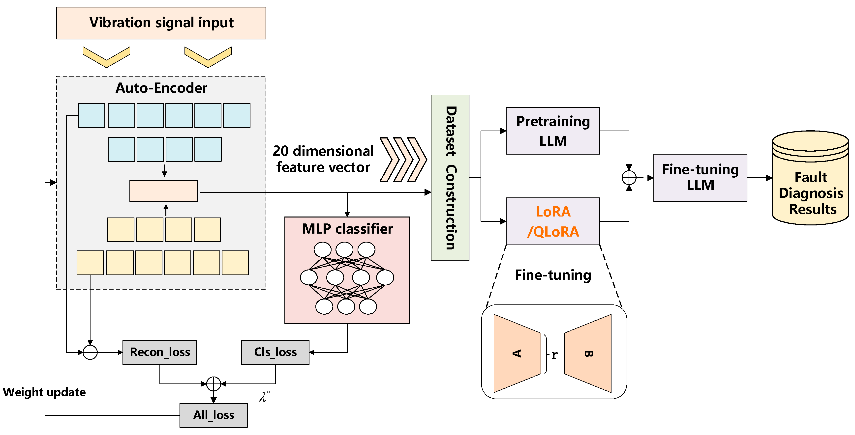
The overall diagnostic framework follows a two-stage paradigm of “feature extraction + LLM classification,” as shown in Figure 1. The core difference between the baseline method and the proposed method lies in the feature extraction module of the first stage, while the LLM diagnostic module in the second stage remains the same for both, ensuring a fair comparison.
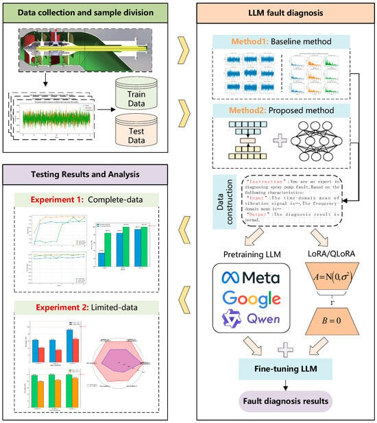
Figure 1.
Overall technical framework of this work.
- Baseline method: The baseline method serves as the experimental benchmark. This approach follows the idea proposed by Tao et al. [16]. It aims to evaluate the diagnostic performance when combining mature, traditional signal processing techniques with cutting-edge LLMs. Its core idea is to leverage expert knowledge to manually extract 24 validated statistical features from the raw signal (in both time and frequency domains) and then convert these structured numerical features into a natural language format that an LLM can understand. In this work, we select a total of 20 features (time and frequency domain), having removed several redundant features.
- Proposed SAE-LLM method: This approach directly inputs raw vibration signal segments into a pre-trained SAE encoder, which automatically extracts a 20-dimensional deep feature vector. This feature vector is then fed into an LLM for fine-tuning to perform fault classification.
The specific approach to SAE-LLM is described in the next section, The feature vectors produced by both baseline method and proposed method are subsequently textualized and used for parameter-efficient fine-tuning of the LLM, ultimately achieving precise end-to-end fault state identification.
3.2. Proposed Method: LLM Diagnosis Framework Based on Supervised Autoencoder
3.2.1. Method Overview
To address the problem that manual feature extraction in time and frequency domains relies on expert knowledge, is time-consuming, and has limited generalization, we propose a new method based on a supervised autoencoder (SAE) for automated feature learning. The core advantage of this method is its ability to use label information to guide the feature learning process, automatically extracting low-dimensional and robust features from raw vibration signals that are optimal for the fault classification task. This provides higher information density and more discriminative inputs for the subsequent LLM fine-tuning.
3.2.2. Framework Composition
The technical framework of this method is illustrated in Figure 2, and the process is divided into three steps:
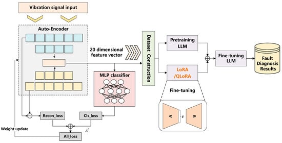
Figure 2.
LLM diagnostic framework based on supervised autoencoder.
- SAE model training: Design and train an SAE model. This model takes raw signal segments as input and optimizes both the reconstruction and classification objectives simultaneously.
- Automated feature extraction: Use the trained SAE encoder to directly map new vibration signal segments to a 20-dimensional deep feature vector.
- Feature textualization and LLM fine-tuning: Following the same approach as the baseline method, textualize the feature vector extracted by the SAE and use it to fine-tune the LLM.
3.2.3. Structure of the Supervised Autoencoder (SAE)
The SAE is an improved model based on the standard autoencoder (AE), and its structure consists of three key components: an encoder (E), a decoder (D), and a classifier (C). The encoder E is a multi-layer neural network that compresses the high-dimensional input data into a low-dimensional latent variable. In this work, the latent dimension is 20. The decoder D has a structure roughly symmetric to the encoder; its task is to take the latent variable and attempt to reconstruct the original input . The classifier C is an independent multi-layer neural network that takes the encoder’s latent variable as input and predicts the fault category of the sample.
The essence of the SAE lies in its unique loss function, which consists of a reconstruction loss and a classification loss. Specifically, the joint loss is given by
where is the reconstruction loss of the model, is the classification loss, and is a hyperparameter that balances these two terms. We use mean squared error (MSE) to measure the difference between the input and the reconstructed output . This loss term forces the features learned by the encoder to retain sufficient information for reconstructing the original signal, ensuring the completeness of the feature information. We use the cross-entropy loss to measure the difference between the classifier’s predicted category and the true label .This loss term directly supervises the encoder’s parameter updates via backpropagation, driving the extracted features to have high separability between different fault categories.
By optimizing this joint loss function, the SAE learns a feature space that both preserves the structural information of the original signal and selectively amplifies patterns related to fault categories. After training is complete, the decoder and classifier parts are discarded, and only the trained encoder is retained as an efficient, automated feature extractor.
3.3. LLM Fine-Tuning Technique
The feature vectors extracted by both methods ultimately feed into a unified LLM-based diagnostic backend. As mentioned in Section 3.1, we convert the 20-dimensional time/frequency features (from the baseline) and the 20-dimensional SAE features into text sequences using a fixed question–answer prompt template, so that the LLM can process them. An example format of the input text sequence is shown in Figure 3.
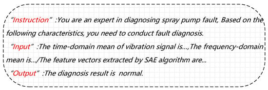
Figure 3.
LLM diagnostic model input text sequence format.
To efficiently adapt the LLM to our diagnostic task, we employ a supervised fine-tuning (SFT) strategy. Given the enormous number of parameters in pre-trained LLMs, we use the LoRA technique [35] for fine-tuning. The core idea of LoRA is to freeze the original weights of the pre-trained LLM and inject a “bypass” composed by two low-rank matrices (often denoted as ,) in parallel to each layer. During fine-tuning, the original model weights are frozen (not updated); only the parameters of the low-rank matrices A and B are trained. The effective weight update for each layer is then given by the product AB, as follows:
Because the rank , the total number of trainable parameters is greatly reduced. This allows for fast and efficient fine-tuning of large models on standard hardware while maintaining high performance.
4. Experiments and Analysis
This chapter first introduces the dataset used in the experiments and then carries out comprehensive performance comparisons and analyses between the baseline method and the proposed SAE-LLM method under two carefully designed experimental scenarios.
4.1. Experimental Platform and Data Collection
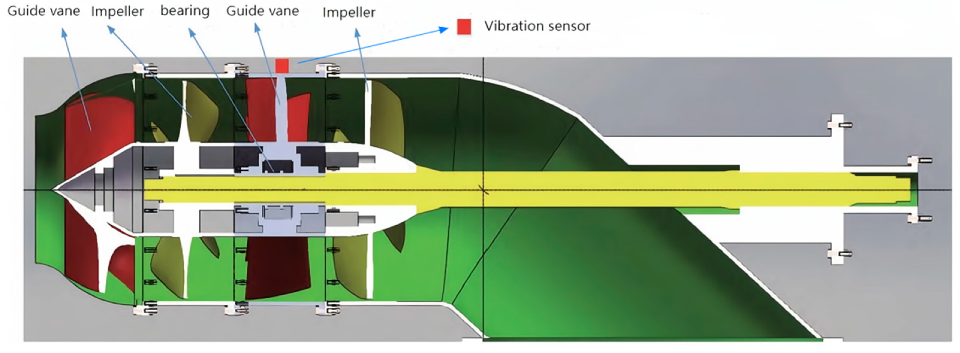
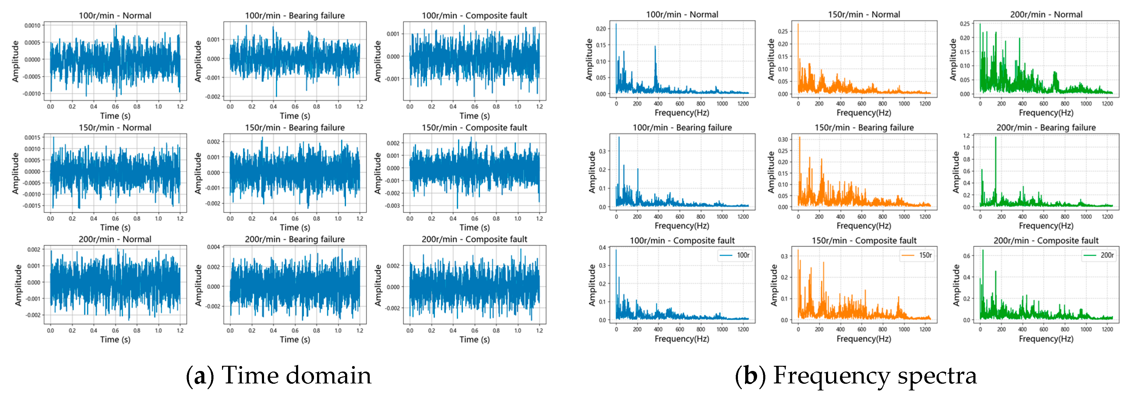
The experimental data were collected from a waterjet pump test bench. The pump fault testing setup and measurement points are shown in Figure 4. An accelerometer was mounted on the guide vane casing of the pump body to collect vibration signals during pump operation, with a sampling frequency of 2500 Hz. The size of each sample is 3000. The experiment includes operating data for the pump under three different health states: Normal (all pump components functioning normally); Bearing Fault (a fault in one of the pump’s support bearings); and Compound Fault (bearing failure superimposed with impeller imbalance and axial pump deviation). Different fault types of waterjet propulsion pump are shown in Figure 5. To simulate different vessel speeds, for each health state we collected data at three different pump rotational speeds: 100 rpm, 150 rpm, and 200 rpm. Table 1 details the dataset composition. For clarity, we also show time-domain waveforms and spectra of the data under different conditions and fault modes in Figure 6.
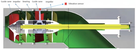
Figure 4.
Illustration of the waterjet pump test setup and sensor placement.

Figure 5.
Different fault types of waterjet propulsion pump.

Table 1.
Experimental dataset description.
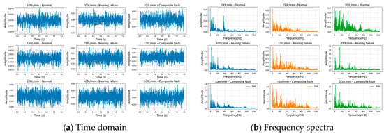
Figure 6.
Comparison of time domain waveforms and frequency spectra.
4.2. Experimental Parameter Settings
All models were implemented in the PyTorch framework (version 2.6.0+cu124). Experiments were conducted on a server equipped with an NVIDIA A100 GPU. The key hyperparameters for the models and SAE model structure settings are given in Table 2 and Table 3 respectively.

Table 2.
Key hyperparameter settings of the models.

Table 3.
SAE model structure settings.
In Table 2, lora_rank denotes the rank of the low-rank matrices; lora_alpha represents the scaling factor for LoRA fine-tuning, controlling the contribution level of the low-rank matrices to the original weights; per_device_train_batch_size indicates the training batch size per device (GPU); gradient_accumulation_steps specifies the number of gradient accumulation steps during LoRA fine-tuning. The effective batch size is calculated as per_device_train_batch_size × gradient_accumulation_steps = 16.
In Table 3, this SAE model structure gradually compresses the high-dimensional input to the low-dimensional feature vector through the deep encoder, so that the model can learn high-quality feature representation. Adding batch normalization and dropout in each layer not only accelerates convergence, but also effectively alleviates over fitting. The decoder reconstructs the input symmetrically, and guarantees the complete expression of the feature vector to the original data through the reconstruction error. The parallel classifier uses the feature vector for classification guidance, and combines self-supervised reconstruction with supervised classification, so as to improve the reconstruction quality and classification performance.
4.3. Experiment 1: Full Data Direct Diagnosis Performance Analysis
To evaluate the diagnostic accuracy of the proposed SAE-LLM method compared to the baseline under full data conditions, data from all three operating conditions (100, 150, 200 rpm) were combined. The combined dataset was split into a training set (80%) and a test set (20%). We selected three pre-trained LLMs with comparable parameter scales: Llama-3.2-3B-Instruct, Qwen-2.5-3B-Instruct, and Gemma-3-4B-Instruct. For each LLM, we fine-tuned it using features obtained by each of the two feature extraction methods (baseline manual features and proposed SAE features) and then evaluated the diagnosis accuracy on the test set using the fine-tuned models.
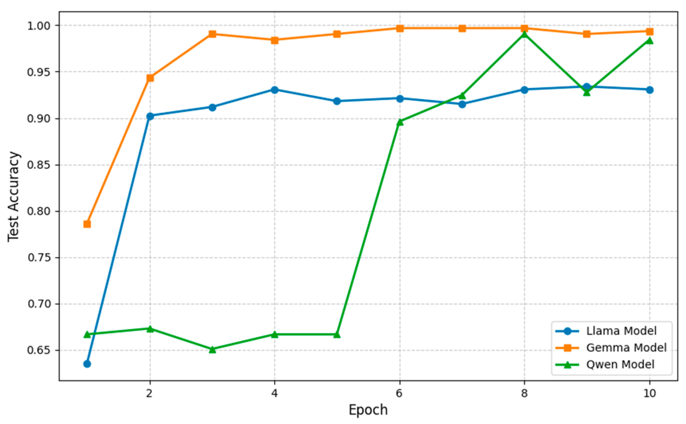
The baseline method’s direct diagnosis accuracy on each LLM is shown in Table 4 and Figure 7, with the confusion matrices at epoch 10 shown in Figure 8. The baseline method achieves reasonable accuracy on all tested LLMs, with the highest accuracy on Gemma-3-4B-Instruct and the lowest on Llama-3.2-3B-Instruct.

Table 4.
Direct diagnosis accuracy of the baseline method on each LLM.
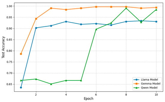
Figure 7.
Diagnostic accuracy of the baseline method on different LLMs.

Figure 8.
Confusion matrices of the baseline method on different LLMs (epoch = 10).
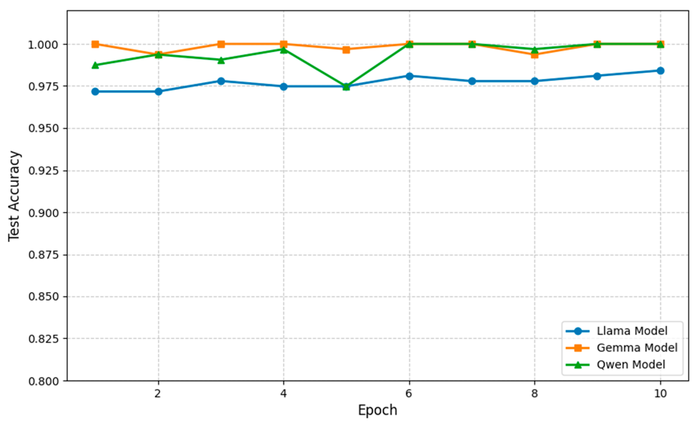
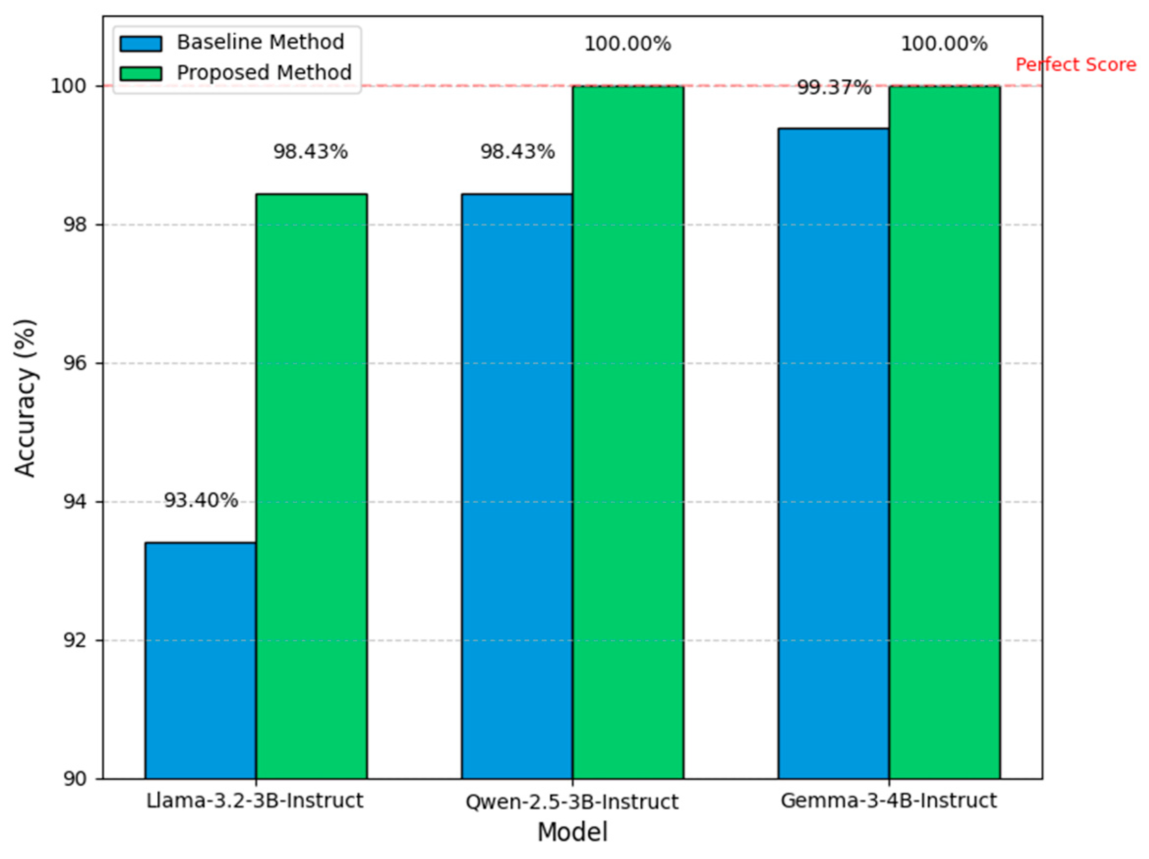
Next, the proposed SAE-LLM method’s direct diagnosis accuracy on each LLM is presented in Table 5 and Figure 9, with a comparison to the baseline method shown in Figure 10. We observe that the SAE-based method achieves higher accuracy than the baseline on all LLMs. In particular, on Llama-3.2-3B-Instruct, after 10 training epochs, the accuracy improves by about 5% compared to the baseline, demonstrating a substantial enhancement in diagnostic precision. These results indicate that the 20-dimensional deep feature vectors automatically extracted by the SAE have stronger representation and discriminative power than the manually extracted time–frequency features.

Table 5.
Direct diagnosis accuracy of the SAE-LLM method on each LLM.
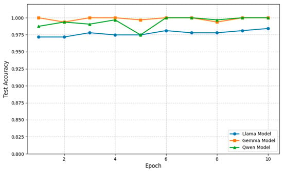
Figure 9.
Diagnostic accuracy of SAE-LLM method on different LLMs.

Figure 10.
Comparison of diagnostic accuracy between the baseline and SAE-LLM methods on different LLMs (epoch = 10).
4.4. Experiment 2: Limited Data Transfer Diagnosis Performance Analysis
In practical engineering applications, obtaining fault data is often costly and limited. To evaluate the model’s generalization and transfer learning ability under sparse data and changing operating conditions, we simulate a typical industrial scenario: for example, the model is primarily trained on conditions A (e.g., 100 rpm) and B (e.g., 150 rpm), but only a small amount of data is available for the target condition C (e.g., 200 rpm). We set up two few-shot scenarios with limited data:
- Scenario a: Fine-tune the pre-trained LLM using all the data from conditions A and B, as well as 10% of the data from condition C, then test on the remaining 90% of condition C.
- Scenario b: Fine-tune the pre-trained LLM using only 10% of the data from condition C as the training set, then test on the remaining 90% of condition C.
We compare the diagnostic accuracy of the baseline method and the SAE-LLM method under these two scenarios; the method achieving higher accuracy is considered to have stronger few-shot learning and transfer generalization capability.
As established in Section 4.3, the Gemma-3-4B-Instruct model shows the best performance, so we use it as the pre-trained LLM in this experiment. The baseline method’s transfer diagnosis accuracies under the two few-shot scenarios are shown in Table 6 and Figure 11. The results indicate that, compared to directly fine-tuning with limited few-shot data, training on source domain data (conditions A and B) and then fine-tuning with the few-shot data from condition C yields a higher diagnosis accuracy.

Table 6.
Baseline method few-shot transfer diagnosis accuracy.
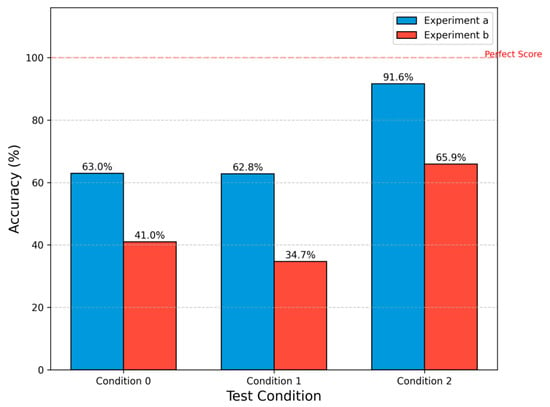
Figure 11.
Transfer diagnosis accuracy of the baseline method under few-shot scenarios.
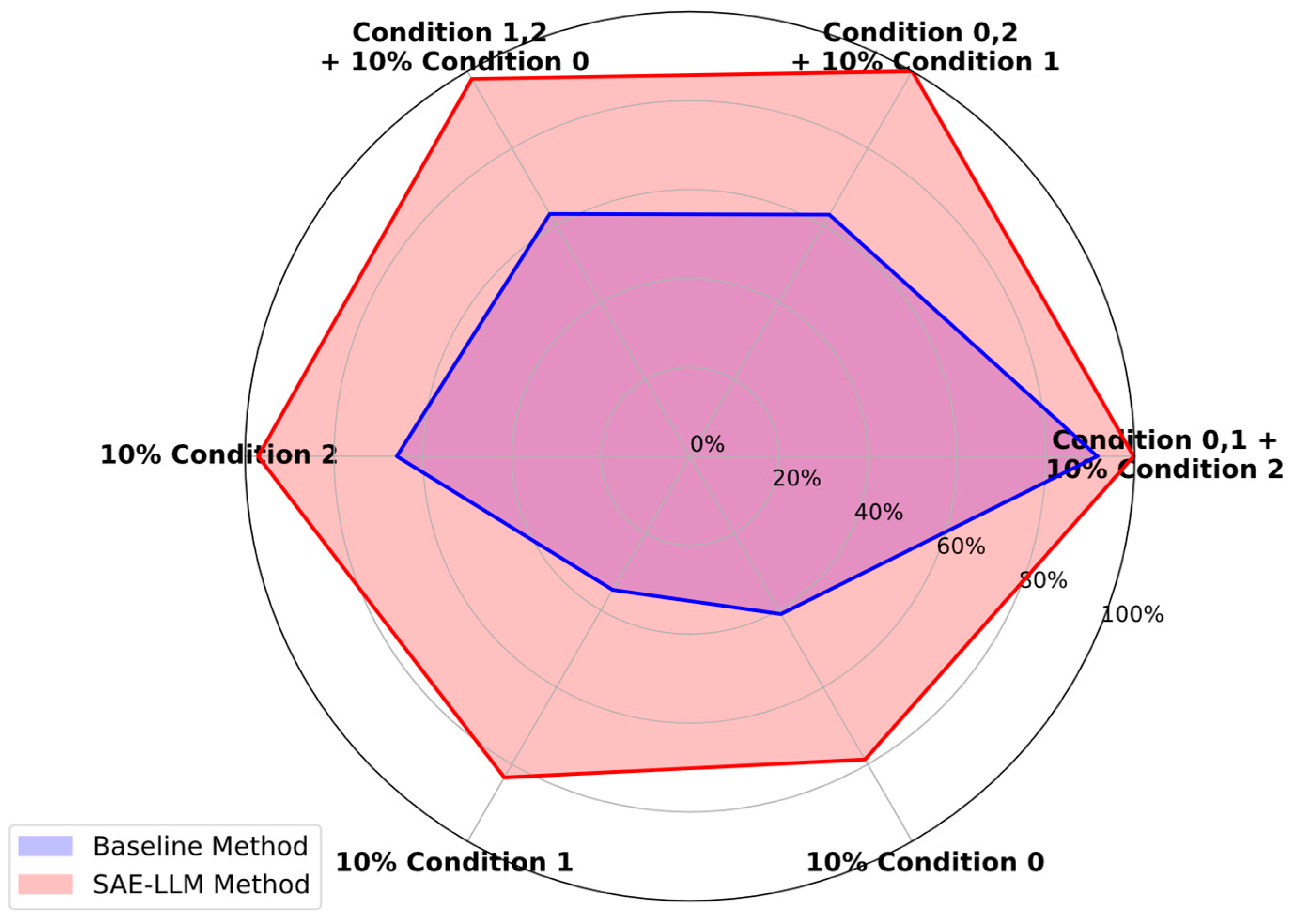
The proposed SAE-LLM method’s transfer diagnosis accuracies under the two few-shot scenarios are shown in Table 7 and Figure 12, with a comparison to the baseline in Figure 13. The results show that in both scenarios, the proposed SAE-LLM method exhibits significant advantages. In scenario a, the features learned by the SAE using source domain data appear to be somewhat invariant to operating conditions; with only a small number of target-domain samples, the model quickly adapts to the new condition. In the limited-data scenario b, the SAE method—trained on very few samples—still achieves higher accuracy than the baseline. This demonstrates that the automatically learned feature representations from the SAE are not only highly discriminative but also more robust and generalizable. They capture the essential physical patterns of the faults, rather than surface phenomena specific to particular conditions, thereby showing strong adaptability in the face of changing conditions and data scarcity.

Table 7.
SAE-LLM method’s few-shot transfer diagnosis accuracy.
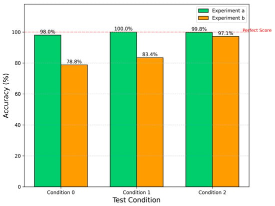
Figure 12.
Transfer diagnosis accuracy of the SAE-LLM method under few-shot scenarios.
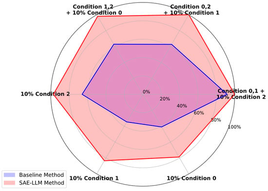
Figure 13.
Comparison of few-shot transfer diagnosis accuracy between baseline and SAE-LLM methods.
5. Conclusions
In this paper, we proposed a novel intelligent diagnostic framework that integrates a supervised autoencoder (SAE) with a large language model (LLM) for ship waterjet pump fault diagnosis. The framework automatically learns high-discriminative deep features oriented towards the diagnostic task from raw vibration signals via the SAE and uses these features as high-quality inputs to the LLM for efficient and precise fault classification.
The main findings and contributions of this research can be summarized as follows:
- Automated, high-accuracy diagnostic paradigm: We successfully constructed and validated a new automated diagnostic paradigm. Experimental results show that, in both data-rich direct diagnosis scenarios and limited-data, cross-condition transfer scenarios, the proposed SAE-LLM framework significantly outperforms the baseline method based on manual features in terms of diagnostic accuracy.
- Critical role of task-oriented feature learning: We demonstrated that learning task-specific features is crucial for the LLM’s diagnostic performance. Through the SAE’s supervised learning mechanism, the extracted features are learned automatically, and more importantly, their inherent fault discriminability far exceeds that of manual statistical features. This allows the LLM to fully exploit its classification potential, especially in distinguishing confusing compound faults.
- Strong generalization under practical industrial conditions: The excellent performance of the proposed framework in limited data and transfer learning experiments demonstrates its strong generalization ability and data efficiency. This provides an effective technical solution for addressing the common issues of data scarcity and varying operating conditions in intelligent industrial maintenance.
This framework has significant practical implications for real-world industrial deployments. Its automated feature learning and diagnosis reduce reliance on time-consuming manual feature engineering, making it more accessible for industrial settings where rapid and accurate fault diagnosis is crucial. The data efficiency and strong generalization ability also suit it for environments with varying operating conditions and limited data, common in industrial applications. Furthermore, the framework shows promise for generalization to other rotating machinery like turbines, compressors, or engines. By retraining the SAE on vibration data from different machinery types and fine-tuning the LLM accordingly, the framework can be extended to provide effective diagnostic solutions across a broader range of equipment.
Despite these positive results, some limitations remain and merit further exploration. First, this study used only a single vibration signal, Vibration signals in real-world industrial environments may be corrupted by noise or missing values, which can affect the performance of the SAE in extracting meaningful features. Future work could explore fusing multi-modal sensor information (such as pressure and temperature data) to build a more comprehensive equipment health profile. Second, the fine-tuning of the LLM presents its own set of challenges, including the risk of overfitting to the specific fault patterns in the training data. Advanced parameter-efficient fine-tuning techniques could be explored to enhance the LLM’s adaptability and generalization. Finally, applying this framework to a wider range of rotating machinery (such as aero-engines, wind turbines, etc.) to validate its generality will be an important direction for future research. Moreover, coupling diagnostic models like ours with intelligent predictive maintenance systems (e.g., sequential multi-objective multi-agent reinforcement learning approach for predictive maintenance proposed by Chen et al. [36]) may unlock autonomous maintenance pipelines.
Author Contributions
Conceptualization and methodology, Z.L.; validation and formal analysis, H.X. and T.Z.; investigation and data curation, G.L.; writing—original draft preparation, Z.L.; writing—review and editing, T.Z. and H.X. All authors have read and agreed to the published version of the manuscript.
Funding
This research was funded by National Defense Basic Scientific Research Program grant number 2022601C009.
Data Availability Statement
Data are unavailable due to privacy or ethical restrictions. Specifically, the data are subject to commercial and confidentiality restrictions, which makes them temporarily unavailable for public access.
Conflicts of Interest
The authors declare no conflicts of interest.
References
- Molland, A.F.; Turnock, S.R.; Hudson, D.A. Ship Resistance and Propulsion; Cambridge University Press: Cambridge, UK, 2017. [Google Scholar]
- Gong, J.; Guo, C.; Wang, C.; Wu, T.; Song, K. Analysis of waterjet-hull interaction and its impact on the propulsion performance of a four-waterjet-propelled ship. Ocean. Eng. 2019, 180, 211–222. [Google Scholar] [CrossRef]
- Li, G.; Geng, H.; Xie, F.; Xu, C.; Xu, Z. Ensemble Deep Transfer Learning Method for Fault Diagnosis of Waterjet Pump Under Variable Working Conditions. Ship Boat 2025, 36, 103. [Google Scholar]
- Lei, Y.; Yang, B.; Jiang, X.; Jia, F.; Li, N.; Nandi, A.K. Applications of machine learning to machine fault diagnosis: A review and roadmap. Mech. Syst. Signal Process. 2020, 138, 106587. [Google Scholar] [CrossRef]
- Randall, R.B.; Antoni, J. Rolling element bearing diagnostics—A tutorial. Mech. Syst. Signal Process. 2011, 25, 485–520. [Google Scholar] [CrossRef]
- Zhang, R.; Tao, H.; Wu, L.; Guan, Y. Transfer learning with neural networks for bearing fault diagnosis in changing working conditions. IEEE Access 2017, 5, 14347–14357. [Google Scholar] [CrossRef]
- Hoang, D.-T.; Kang, H.-J. A survey on deep learning based bearing fault diagnosis. Neurocomputing 2019, 335, 327–335. [Google Scholar] [CrossRef]
- Lv, F.; Wen, C.; Bao, Z.; Liu, M. Fault diagnosis based on deep learning. In Proceedings of the 2016 American Control Conference (ACC), Boston, MA, USA, 6–8 July 2016; pp. 6851–6856. [Google Scholar]
- Zhang, W.; Li, C.; Peng, G.; Chen, Y.; Zhang, Z. A deep convolutional neural network with new training methods for bearing fault diagnosis under noisy environment and different working load. Mech. Syst. Signal Process. 2018, 100, 439–453. [Google Scholar] [CrossRef]
- Pan, H.; He, X.; Tang, S.; Meng, F. An improved bearing fault diagnosis method using one-dimensional CNN and LSTM. Stroj. Vestn. J. Mech. Eng. 2018, 64, 443–453. [Google Scholar]
- Chen, X.; Yang, R.; Xue, Y.; Huang, M.; Ferrero, R.; Wang, Z. Deep transfer learning for bearing fault diagnosis: A systematic review since 2016. IEEE Trans. Instrum. Meas. 2023, 72, 1–21. [Google Scholar] [CrossRef]
- Ding, Y.; Ma, L.; Ma, J.; Wang, C.; Lu, C. A generative adversarial network-based intelligent fault diagnosis method for rotating machinery under small sample size conditions. IEEE Access 2019, 7, 149736–149749. [Google Scholar] [CrossRef]
- Brown, T.; Mann, B.; Ryder, N.; Subbiah, M.; Kaplan, J.D.; Dhariwal, P.; Neelakantan, A.; Shyam, P.; Sastry, G.; Askell, A. Language models are few-shot learners. Adv. Neural Inf. Process. Syst. 2020, 33, 1877–1901. [Google Scholar]
- Chang, Y.; Wang, X.; Wang, J.; Wu, Y.; Yang, L.; Zhu, K.; Chen, H.; Yi, X.; Wang, C.; Wang, Y. A survey on evaluation of large language models. ACM Trans. Intell. Syst. Technol. 2024, 15, 1–45. [Google Scholar] [CrossRef]
- Naveed, H.; Khan, A.U.; Qiu, S.; Saqib, M.; Anwar, S.; Usman, M.; Akhtar, N.; Barnes, N.; Mian, A. A comprehensive overview of large language models. ACM Trans. Intell. Syst. Technol. 2025. just accepted. [Google Scholar] [CrossRef]
- Tao, L.; Liu, H.; Ning, G.; Cao, W.; Huang, B.; Lu, C. LLM-based framework for bearing fault diagnosis. Mech. Syst. Signal Process. 2025, 224, 112127. [Google Scholar] [CrossRef]
- Peng, Z.K.; Chu, F. Application of the wavelet transform in machine condition monitoring and fault diagnostics: A review with bibliography. Mech. Syst. Signal Process. 2004, 18, 199–221. [Google Scholar] [CrossRef]
- Zio, E. Prognostics and Health Management (PHM): Where are we and where do we (need to) go in theory and practice. Reliab. Eng. Syst. Saf. 2022, 218, 108119. [Google Scholar] [CrossRef]
- Chen, Z.; He, G.; Li, J.; Liao, Y.; Gryllias, K.; Li, W. Domain adversarial transfer network for cross-domain fault diagnosis of rotary machinery. IEEE Trans. Instrum. Meas. 2020, 69, 8702–8712. [Google Scholar] [CrossRef]
- Li, F.; Tang, T.; Tang, B.; He, Q. Deep convolution domain-adversarial transfer learning for fault diagnosis of rolling bearings. Measurement 2021, 169, 108339. [Google Scholar] [CrossRef]
- Li, T.; Zhao, Z.; Sun, C.; Yan, R.; Chen, X. Domain adversarial graph convolutional network for fault diagnosis under variable working conditions. IEEE Trans. Instrum. Meas. 2021, 70, 3515010. [Google Scholar] [CrossRef]
- Li, Y.; Song, Y.; Jia, L.; Gao, S.; Li, Q.; Qiu, M. Intelligent fault diagnosis by fusing domain adversarial training and maximum mean discrepancy via ensemble learning. IEEE Trans. Ind. Inform. 2020, 17, 2833–2841. [Google Scholar] [CrossRef]
- Wen, L.; Gao, L.; Li, X. A new deep transfer learning based on sparse auto-encoder for fault diagnosis. IEEE Trans. Syst. Man Cybern. Syst. 2017, 49, 136–144. [Google Scholar] [CrossRef]
- Li, Y.-F.; Wang, H.; Sun, M. ChatGPT-like large-scale foundation models for prognostics and health management: A survey and roadmaps. Reliab. Eng. Syst. Saf. 2024, 243, 109850. [Google Scholar] [CrossRef]
- Tao, L.; Li, S.; Liu, H.; Huang, Q.; Ma, L.; Ning, G.; Chen, Y.; Wu, Y.; Li, B.; Zhang, W. An outline of Prognostics and health management Large Model: Concepts, Paradigms, and challenges. Mech. Syst. Signal Process. 2025, 232, 112683. [Google Scholar] [CrossRef]
- Hinton, G.E.; Zemel, R. Autoencoders, minimum description length and Helmholtz free energy. Adv. Neural Inf. Process. Syst. 1993, 6, 3–10. [Google Scholar]
- Lu, C.; Wang, Z.-Y.; Qin, W.-L.; Ma, J. Fault diagnosis of rotary machinery components using a stacked denoising autoencoder-based health state identification. Signal Process. 2017, 130, 377–388. [Google Scholar] [CrossRef]
- Sun, M.; Wang, H.; Liu, P.; Huang, S.; Fan, P. A sparse stacked denoising autoencoder with optimized transfer learning applied to the fault diagnosis of rolling bearings. Measurement 2019, 146, 305–314. [Google Scholar] [CrossRef]
- Ding, N.; Qin, Y.; Yang, G.; Wei, F.; Yang, Z.; Su, Y.; Hu, S.; Chen, Y.; Chan, C.-M.; Chen, W. Parameter-efficient fine-tuning of large-scale pre-trained language models. Nat. Mach. Intell. 2023, 5, 220–235. [Google Scholar] [CrossRef]
- He, J.; Zhou, C.; Ma, X.; Berg-Kirkpatrick, T.; Neubig, G. Towards a unified view of parameter-efficient transfer learning. arXiv 2021, arXiv:2110.04366. [Google Scholar]
- Han, Z.; Gao, C.; Liu, J.; Zhang, J.; Zhang, S.Q. Parameter-efficient fine-tuning for large models: A comprehensive survey. arXiv 2024, arXiv:2403.14608. [Google Scholar]
- Li, X.L.; Liang, P. Prefix-tuning: Optimizing continuous prompts for generation. arXiv 2021, arXiv:2101.00190. [Google Scholar]
- Houlsby, N.; Giurgiu, A.; Jastrzebski, S.; Morrone, B.; De Laroussilhe, Q.; Gesmundo, A.; Attariyan, M.; Gelly, S. Parameter-efficient transfer learning for NLP. In Proceedings of the International Conference on Machine Learning, Long Beach, CA, USA, 9–15 June 2019; pp. 2790–2799. [Google Scholar]
- Lester, B.; Al-Rfou, R.; Constant, N. The power of scale for parameter-efficient prompt tuning. arXiv 2021, arXiv:2104.08691. [Google Scholar]
- Hu, E.J.; Shen, Y.; Wallis, P.; Allen-Zhu, Z.; Li, Y.; Wang, S.; Wang, L.; Chen, W. Lora: Low-rank adaptation of large language models. ICLR 2022, 1, 3. [Google Scholar]
- Chen, Y.; Liu, C. Sequential multi-objective multi-agent reinforcement learning approach for system predictive maintenance of turbofan engine. Adv. Eng. Inform. 2025, 67, 103553. [Google Scholar] [CrossRef]
Disclaimer/Publisher’s Note: The statements, opinions and data contained in all publications are solely those of the individual author(s) and contributor(s) and not of MDPI and/or the editor(s). MDPI and/or the editor(s) disclaim responsibility for any injury to people or property resulting from any ideas, methods, instructions or products referred to in the content. |
© 2025 by the authors. Licensee MDPI, Basel, Switzerland. This article is an open access article distributed under the terms and conditions of the Creative Commons Attribution (CC BY) license (https://creativecommons.org/licenses/by/4.0/).


