The Research on Multi-Objective Maintenance Optimization Strategy Based on Stochastic Modeling

Abstract

The traditional approach that separates remaining useful life prediction from maintenance strategy design often fails to support efficient decision-making. Effective maintenance requires a comprehensive consideration of prediction accuracy, cost control, and equipment safety. To address this issue, this paper proposes a multi-objective maintenance optimization method based on stochastic modeling. First, a multi-sensor data fusion technique is developed, which maps multidimensional degradation signals into a composite degradation state indicator using evaluation metrics such as monotonicity, tendency, and robustness. Then, a linear Wiener process model is established to characterize the degradation trajectory of equipment, and a closed-form analytical solution of its reliability function is derived. On this basis, a multi-objective optimization model is constructed, aiming to maximize equipment safety and minimize maintenance cost. The proposed method is validated using the NASA aircraft engine degradation dataset. The experimental results demonstrate that, while ensuring system reliability, the proposed approach significantly reduces maintenance costs compared to traditional periodic maintenance strategies, confirming its effectiveness and practical value.

1. Introduction

With the continuous advancement of intelligent high-end equipment, ensuring operational reliability and cost-effective maintenance over the entire life cycle has become a central issue in industrial operation and maintenance management. During long-term service, critical components inevitably undergo multiple degradation mechanisms, such as fatigue, wear, and corrosion, which progressively deteriorate system performance and pose risks to stability and safety. Developing scientific and rational maintenance strategies under the premise of reliable operation has thus emerged as a key topic for achieving sustainable system performance and reducing operational costs [1]. Traditional maintenance strategies are typically based on fixed intervals or heuristic rules, lacking the integration of real-time monitoring data and falling short in adapting to complex degradation behaviors under varying operational conditions. Therefore, establishing data-driven approaches for life modeling and maintenance optimization is of great theoretical and engineering significance for achieving intelligent predictive maintenance [2,3,4].

Remaining useful life (RUL) prediction, a core task in predictive maintenance, has garnered significant research interest in recent years [5]. By constructing mathematical models of degradation processes and inferring the current technical state of equipment, RUL prediction provides quantitative support for maintenance scheduling, component replacement, and risk prevention. Maintenance strategies formulated based on RUL predictions have become a key direction in intelligent operation and maintenance. Existing studies can be broadly classified into two categories: physics-based models and data-driven approaches. The former relies on damage evolution models or physical degradation equations and is suitable for systems with well-understood failure mechanisms. The latter leverages sensor signals and historical data for feature extraction and modeling, offering strong adaptability and real-time performance.

Recent research in maintenance strategy optimization has focused on improving system reliability, reducing maintenance costs, and enhancing decision-making methodologies [6,7,8]. The research trend has shifted from traditional time-based maintenance to data-driven condition-based maintenance, incorporating techniques from reliability analysis, Markov processes, probabilistic statistics, optimization theory, and machine learning to enhance decision accuracy and scientific rigor [9,10,11]. For instance, You [12] proposed a time- or state-based maintenance method using weighted averaging to select maintenance actions. Arts et al. [13] developed periodic and condition-based maintenance strategies for wind turbines and marine systems to minimize maintenance and downtime costs. Ding et al. [14] introduced a maintenance decision model to enhance system availability and reliability. Zhu et al. [15] proposed a preventive maintenance strategy based on both time and condition, targeting maintenance time cost optimization.

Moreover, some recent studies have started to integrate RUL prediction with maintenance strategy optimization, aiming to construct decision-making frameworks that consider both reliability and cost-effectiveness. In terms of RUL prediction, Wang et al. [16] proposed a two-stage Wiener process model with adaptive drift to account for internal degradation mechanisms and time-varying operational conditions. They derived the probability density function of the RUL and extended the model to include unit heterogeneity and state uncertainty at the change point. Jiang et al. [17] addressed the uncertainty in multi-sensor monitoring data during degradation by proposing a multi-performance indicator fusion method. They mapped multidimensional sensor signals into a one-dimensional composite degradation indicator and used an ensemble of three statistical models for RUL estimation. These studies highlight the interpretability of the Wiener process model, which is adopted in this work for further research. In addition, recent studies [18,19,20,21] have further explored advanced multi-sensor data fusion techniques to enhance the accuracy and robustness of predictive maintenance. Effectively integrating multi-sensor data can significantly enhance equipment health assessments and support informed decision-making. To this end, this study fully leverages multi-sensor information to achieve these objectives.

In summary, although existing studies have made significant progress in RUL prediction and maintenance decision optimization, several limitations remain. Most of the current research focuses primarily on improving the accuracy of RUL prediction while paying insufficient attention to the coordinated optimization between RUL prediction and maintenance decision-making. In response, this study aims to develop an optimal maintenance decision model that simultaneously considers RUL prediction results and adopts a bi-objective optimization strategy balancing maintenance cost and system availability.

The remainder of this paper is organized as follows: Section 2 introduces the construction of the prognostic model, including the multi-sensor data fusion method, the linear Wiener process model, and the parameter estimation approach. Section 3 presents the maintenance strategy optimization framework, covering the cost-based strategy, availability-based strategy, and a bi-objective coordinated optimization scheme. Section 4 provides the experimental results and discussion, including the dataset description, evaluation index definitions, construction of predictive models, and the optimization results of the proposed maintenance strategies. Finally, Section 5 concludes the paper, summarizing the main findings, limitations, and future research directions.

2. Construction of the Prognostic Model

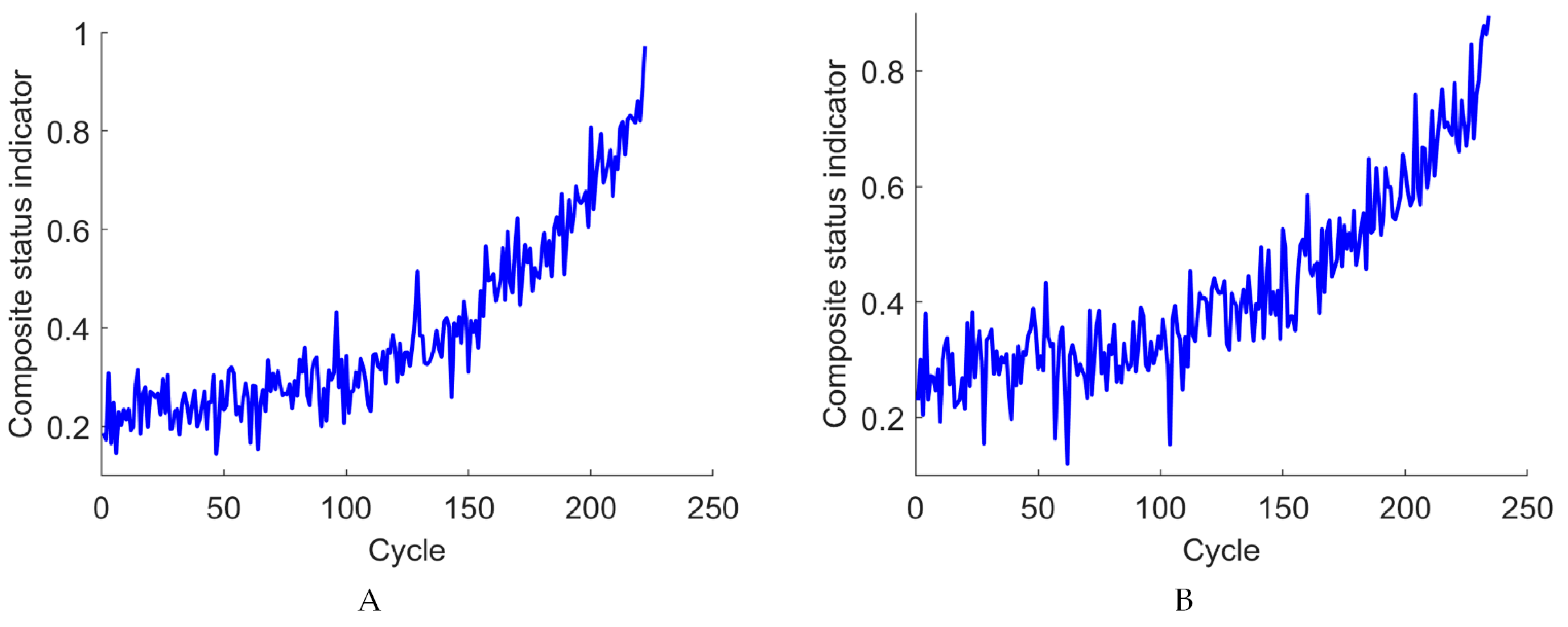
2.1. Multi-Sensor Data Fusion Method

In practical engineering applications, data obtained from a single sensor often suffers from limitations in capturing the comprehensive health status of equipment. To fully leverage multi-source monitoring data and enhance the modelability of equipment degradation states, this study proposes a multi-sensor data fusion method. The approach constructs a unified composite technical state indicator by evaluating the overall quality of the sensor signals using specific assessment metrics. Specifically, monotonicity, trendability, and robustness are employed as evaluation criteria to map multi-dimensional sensor signals into a one-dimensional composite degradation indicator. Assume that the multi-dimensional measurement data from a degrading component is represented as

$$\mathit{X}=\left[\begin{array}{c}{\mathit{X}}_1\\ {\mathit{X}}_2\\ ⋮\\ {\mathit{X}}_m\end{array}\right]=\left[\begin{array}{cccc}{x}_{1,1}& x_{1,2}& \cdots & x_{1,n}\\ x_{2,1}& x_{2,2}& \cdots & x_{2,n}\\ ⋮& ⋮& \ddots & ⋮\\ x_{m,1}& x_{m,2}& \cdots & x_{m,n}\end{array}\right]$$

(1)

where ${\mathit{X}}_m$ denotes the measurement data from the m-th sensor group, and $x_{m,n}$ is the measurement value of the m-th sensor at monitoring time $t_n$.

To eliminate the scale differences among different measurements, min–max normalization is applied as follows:

$${\tilde{\mathit{X}}}_{\mathit{i}}={\displaystyle \frac{{\mathit{X}}_{\mathit{i}}-\min \left({\mathit{X}}_{\mathit{i}}\right)}{\max \left({\mathit{X}}_{\mathit{i}}\right)-\min \left({\mathit{X}}_{\mathit{i}}\right)}},1\le i\le m$$

(2)

In this study, a mapping function $J\left(·\right)$ is constructed to fuse multiple degradation state indicators into a one-dimensional composite technical state indicator. The specific formulation is as follows:

$$\mathit{Y}=J\left(\mathit{\gamma },{\tilde{\mathit{X}}}_{\mathit{i}}\right)=\mathit{\gamma }{\tilde{\mathit{X}}}_{\mathit{i}}={\left[\begin{array}{c}{\gamma }_1\\ {\gamma }_2\\ ⋮\\ {\gamma }_m\end{array}\right]}^T\left[\begin{array}{cccc}{\tilde{x}}_{1,1}& {\tilde{x}}_{1,2}& \cdots & {\tilde{x}}_{1,n}\\ {\tilde{x}}_{2,1}& {\tilde{x}}_{2,2}& \cdots & {\tilde{x}}_{2,n}\\ ⋮& ⋮& \ddots & ⋮\\ {\tilde{x}}_{m,1}& {\tilde{x}}_{m,2}& \cdots & {\tilde{x}}_{m,n}\end{array}\right]={\left[\begin{array}{c}{y}_1\\ y_2\\ ⋮\\ y_n\end{array}\right]}^T,s.t. {\displaystyle \sum _{i=1}^m{\gamma }_i}=1$$

(3)

where $\mathit{\gamma }$ denotes the fusion weight vector for different sensor signals, and ${\gamma }_i$ is the fusion weight associated with the i-th sensor’s measurement. In the fusion process, the fusion weights determine the relative contribution or credibility of each sensor signal to the composite state indicator. A higher fusion weight indicates greater overall quality or trustworthiness of the corresponding sensor.

$$C{e}_i={\displaystyle \sum _{i=1}^3\frac{h_i\left({\mathit{X}}_{\mathit{i}}\right)-{\beta }_{i,\min }}{{\beta }_{i,\max }-{\beta }_{i,\min }}}$$

(4)

$${\widehat{\mathit{\gamma }}}_i={\displaystyle \frac{C{e}_i}{{\displaystyle {\sum }_{i=1}^{3}C{e}_i}}}$$

(5)

where $\widehat{\mathit{\gamma }}$ is the optimal unnormalized fusion score, and $h_1\left(·\right)$, $h_2\left(·\right)$, and $h_3\left(·\right)$ represent the monotonicity, robustness, and trendability evaluation metrics, respectively. ${\beta }_{i,\min }$ and ${\beta }_{i,\max }$ are the minimum and maximum values. This formulation allows different evaluation metrics to be mapped onto the same scale and dimension, enabling effective and interpretable fusion of heterogeneous degradation features.

$$h_1\left(\mathit{Z}\right)={\displaystyle \frac{1}{n-1}}\left|No.ofd/dz>0-No.ofd/dz<0\right|$$

(6)

$$h_2\left(\mathit{Z}\right)={\displaystyle \frac{1}{n}}{\displaystyle \sum _{i=1}^n\exp \left(-\left|\frac{z_i-z_i^{-}}{z_i}\right|\right)}$$

(7)

$$h_3\left(\mathit{Z}\right)={\displaystyle \frac{n\left({\displaystyle {\sum }_{i=1}^n{z}_i{t}_i}\right)-\left({\displaystyle {\sum }_{i=1}^n{z}_i}\right)\left({\displaystyle {\sum }_{i=1}^n{t}_i}\right)}{\sqrt{\left[n{\displaystyle {\sum }_{i=1}^n{\left(z_i\right)}^2}-{\left({\displaystyle {\sum }_{i=1}^n{z}_i}\right)}^2\right]\left[n{\displaystyle {\sum }_{i=1}^n{t}_i^2}-{\left({\displaystyle {\sum }_{i=1}^n{t}_i}\right)}^2\right]}}}$$

(8)

where $t_i$ represents the i-th state monitoring cycle.

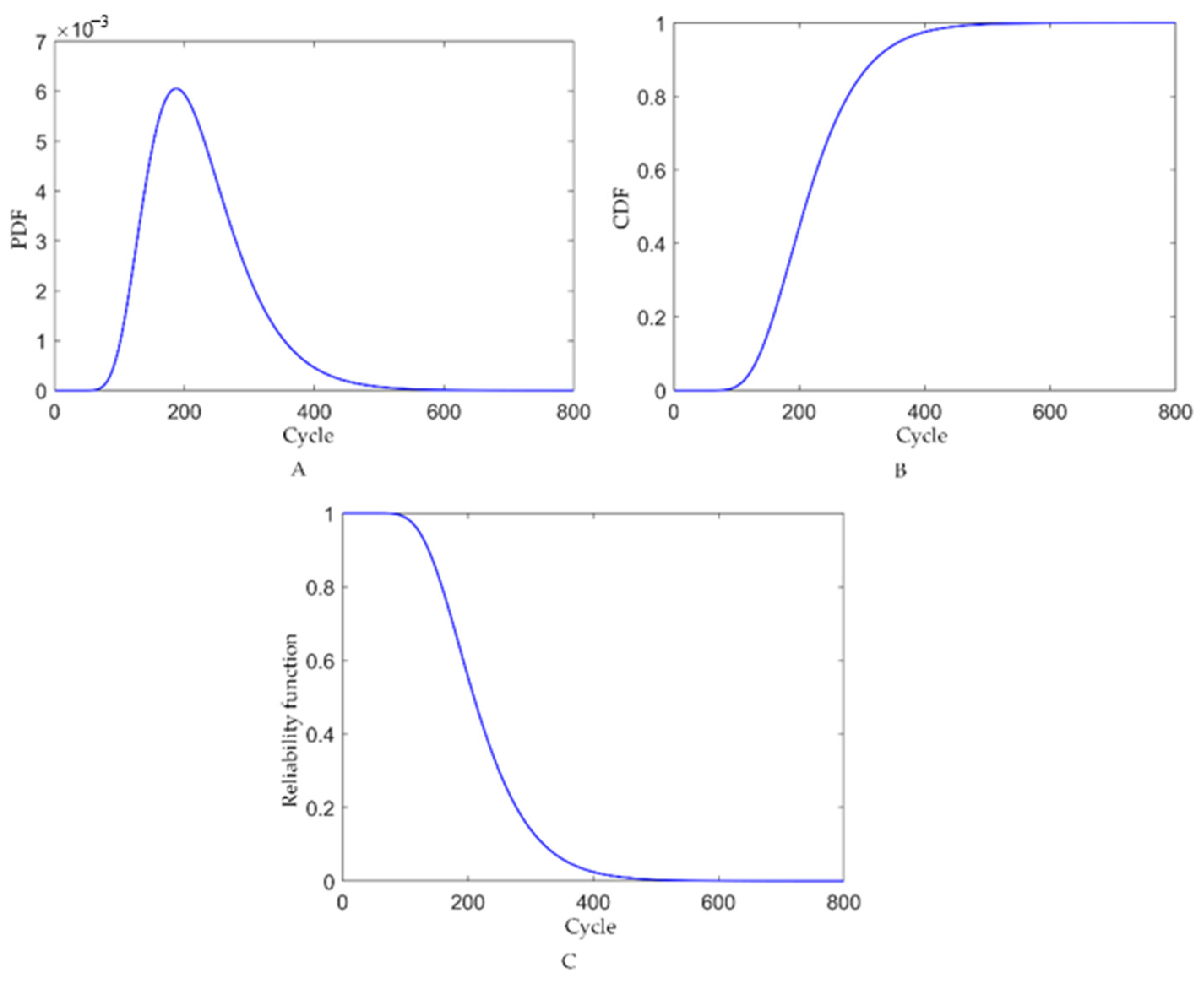
2.2. Linear Wiener Process Model

During the degradation process, the effect of internal deterioration mechanisms often manifests as a two-phase degradation characteristic. The degradation state $Y\left(t\right)$ of the bearing at monitoring time can be expressed as

$$Y\left(t\right)=y_0+\upsilon t+\sigma B\left(t\right)$$

(9)

where $y_0$ is the initial degradation state, $\upsilon$ is the drift coefficient representing the long-term degradation trend, and $\sigma$ is the diffusion coefficient representing the variability introduced by environmental and operational factors. $B\left(·\right)$ is a standard Brownian motion variable used to characterize the temporal uncertainty of the degradation process. Without loss of generality, it is assumed that $y_0=0$.

For simplicity, based on the first passage time modeling principle, failure is assumed to occur when the degradation trajectory first reaches a predefined failure threshold. The failure condition is defined as

$$T=\left\{t:Y\left(t\right)\ge \omega |Y\left(0\right)<\omega \right\}$$

(10)

where $\omega$ denotes the predefined failure threshold.

Under the first passage time framework, the time-to-failure for the linear Wiener process follows an Inverse Gaussian (IG) distribution [22]. When the parameters are known, the closed-form probability density function (PDF) of the time-to-failure is given by

$$f_T\left(t|\sigma ,\upsilon \right)={\displaystyle \frac{\omega }{\sqrt{2\pi {\sigma }^2{t}^3}}}\exp \left[-{\displaystyle \frac{{\left(\omega -\upsilon t\right)}^2}{2{\sigma }^{2}t}}\right]$$

(11)

To enhance the applicability of the prediction model, this study considers the variability in degradation rates among different units caused by factors such as material properties, manufacturing processes, and assembly conditions. Specifically, it is assumed that the drift coefficient is not a fixed constant, but rather a random variable following a normal distribution, denoted as $\upsilon \sim N\left({\mu }_{\upsilon },{\sigma }_{\upsilon }^2\right)$. Based on the law of total probability in Bayesian theory, the PDF of the system’s lifetime under unit-to-unit variability is derived accordingly.

$$\begin{array}{cc}\hfill f_T\left(t|\sigma ,{\mu }_{\upsilon },{\sigma }_{\upsilon }^2\right)& ={\displaystyle {\int }_{-\infty }^{+\infty }{f}_T\left(t|\sigma ,\upsilon \right)}\rho \left(\upsilon \right)d\upsilon \hfill \\ & ={\displaystyle \frac{\omega }{\sqrt{2\pi t^2\left(t{\sigma }^2+t^2{\sigma }_{\upsilon }^2\right)}}}\exp \left[-{\displaystyle \frac{{\left(\omega -{\mu }_{\upsilon }t\right)}^2}{2\left(t{\sigma }^2+t^2{\sigma }_{\upsilon }^2\right)}}\right]\hfill \end{array}$$

(12)

$$\rho \left(\upsilon \right)={\displaystyle \frac{1}{\sqrt{2\pi {\sigma }_{\upsilon }^2}}}\exp \left(-{\displaystyle \frac{{\left(\upsilon -{\mu }_{\upsilon }\right)}^2}{2{\sigma }_{\upsilon }^2}}\right)$$

(13)

By integrating Equation (12), the cumulative distribution function (CDF) and the reliability function of the equipment lifetime, considering unit-to-unit variability, can be derived based on the Bayesian law of total probability. These are given as follows:

$$\begin{array}{l}{F}_T(t|\sigma ,{\mu }_{\upsilon },{\sigma }_{\upsilon }^2)={\displaystyle {\int }_{-\infty }^t{f}_T\left(t|\sigma ,{\mu }_{\upsilon },{\sigma }_{\upsilon }^2\right)}dt\\ =1-\Phi \left({\displaystyle \frac{\omega -{\mu }_{\upsilon }t}{\sqrt{\left({\sigma }_{\upsilon }^2{t}^2+{\sigma }^{2}t\right)}}}\right)+\exp \left({\displaystyle \frac{2{\mu }_{\upsilon }\omega }{{\sigma }^2}}+{\displaystyle \frac{2{\sigma }_{\upsilon }^2{\omega }^2}{{\sigma }^4}}\right)\Phi \left(-{\displaystyle \frac{2{\sigma }_{\upsilon }^2\omega t+{\sigma }^2\left(\omega +{\mu }_{\upsilon }t\right)}{{\sigma }^2\sqrt{{\sigma }_{\upsilon }^2{t}^2+{\sigma }^{2}t}}}\right)\end{array}$$

(14)

$$\begin{array}{l}R\left(t|\sigma ,{\mu }_{\upsilon },{\sigma }_{\upsilon }^2\right)=1-F_T(t|\sigma ,{\mu }_{\upsilon },{\sigma }_{\upsilon }^2)\\ =\Phi \left({\displaystyle \frac{\omega -{\mu }_{\upsilon }t}{\sqrt{\left({\sigma }_{\upsilon }^2{t}^2+{\sigma }^{2}t\right)}}}\right)-\exp \left({\displaystyle \frac{2{\mu }_{\upsilon }\omega }{{\sigma }^2}}+{\displaystyle \frac{2{\sigma }_{\upsilon }^2{\omega }^2}{{\sigma }^4}}\right)\Phi \left(-{\displaystyle \frac{2{\sigma }_{\upsilon }^2\omega t+{\sigma }^2\left(\omega +{\mu }_{\upsilon }t\right)}{{\sigma }^2\sqrt{{\sigma }_{\upsilon }^2{t}^2+{\sigma }^{2}t}}}\right)\end{array}$$

(15)

where $F_T(t|\sigma ,{\mu }_{\upsilon },{\sigma }_{\upsilon }^2)$ is the cumulative distribution function of the equipment’s lifetime under known parameters, and $R\left(t|\sigma ,{\mu }_{\upsilon },{\sigma }_{\upsilon }^2\right)$ is the corresponding reliability function.

2.3. Parameter Estimation

For the sake of simplicity, it is assumed that the equipment is monitored at fixed time intervals. Let the composite degradation state indicator of the equipment at monitoring time $\mathit{T}=\left[t_1,t_2,\cdots t_n\right]$ be denoted as $\mathit{Y}=\left[y_1,y_2,\cdots ,y_n\right]$. According to the independence and Gaussian properties of Wiener process increments, the sequence of observed composite degradation states follows a multivariate normal distribution, which can be expressed as

$$\mathit{Y}\sim MVN\left(\upsilon \mathit{T},{\sigma }_{\upsilon }^2{\mathit{T}}^{\mathbf{\prime }}\mathit{T}+{\sigma }^2\mathit{Q}\right)$$

(16)

where $\mathit{Q}\left(j,k\right)=\min \left(t_j,t_k\right),1\le j,k\le t_n$.

The likelihood function for the degradation state $\mathit{Y}$ is expressed as follows:

$$\begin{array}{l}\ln L\left(\sigma ,{\mu }_{\upsilon },{\sigma }_{\upsilon }^2|\mathit{Y}\right)=-{\displaystyle \frac{n}{2}}\ln \left(2\pi \right)-{\displaystyle \frac{1}{2}}\ln \left|{\sigma }_{\upsilon }^2{\mathit{T}}^{\mathbf{\prime }}\mathit{T}+{\sigma }^2\mathit{Q}\right|\\ -{\displaystyle \frac{1}{2}}\left(\mathit{Y}-\upsilon \mathit{T}\right){\left({\sigma }_{\upsilon }^2{\mathit{T}}^{\mathbf{\prime }}\mathit{T}+{\sigma }^2\mathit{Q}\right)}^{-1}\times {\left(\mathit{Y}-\upsilon \mathit{T}\right)}^{\prime }\end{array}$$

(17)

Taking the derivative of the likelihood function with respect to the unknown parameter ${\mu }_{\upsilon }$, and setting it equal to zero yields

$${\widehat{\mu }}_{\upsilon }={\displaystyle \frac{\mathit{T}{\left({\sigma }_{\upsilon }^2{\mathit{T}}^{\mathbf{\prime }}\mathit{T}+{\sigma }^2\mathit{Q}\right)}^{-1}{\mathit{Y}}^{\mathbf{\prime }}}{\mathit{T}{\left({\sigma }_{\upsilon }^2{\mathit{T}}^{\mathbf{\prime }}\mathit{T}+{\sigma }^2\mathit{Q}\right)}^{-1}{\mathit{T}}^{\mathbf{\prime }}}}$$

(18)

Substituting the above result back into the log-likelihood function gives the profile likelihood function, which is expressed as

$$\begin{array}{l}\ln L\left(\sigma ,{\sigma }_{\upsilon }^2|\mathit{Y}\right)=-{\displaystyle \frac{n}{2}}\ln \left(2\pi \right)-{\displaystyle \frac{1}{2}}\ln \left|{\sigma }_{\upsilon }^2{\mathit{T}}^{\mathbf{\prime }}\mathit{T}+{\sigma }^2\mathit{Q}\right|\\ -{\displaystyle \frac{1}{2}}\left(\mathit{Y}-{\widehat{\mu }}_{\upsilon }\mathit{T}\right){\left({\sigma }_{\upsilon }^2{\mathit{T}}^{\mathbf{\prime }}\mathit{T}+{\sigma }^2\mathit{Q}\right)}^{-1}\times {\left(\mathit{Y}-{\widehat{\mu }}_{\upsilon }\mathit{T}\right)}^{\prime }\end{array}$$

(19)

By maximizing the profile likelihood function, the unknown parameters $\widehat{\sigma }$ and ${\widehat{\sigma }}_{\upsilon }^2$ can be estimated. These estimates can then be substituted back into Equation (10) to obtain the estimate for parameter ${\widehat{\mu }}_{\upsilon }$.

3. Maintenance Strategy Optimization

3.1. Maintenance Strategy Based on Cost Objective

During the operational lifecycle of equipment, controlling maintenance costs is critical to ensuring overall economic efficiency. To achieve this goal, it is essential to construct a mathematical model of maintenance costs to systematically analyze cost trends and economic benefits under different maintenance strategies. Under ideal operating conditions, the average maintenance cost per unit time can be described by the following expression:

$$C\left(t\right)={\displaystyle \frac{C_P+C_C}{T}}$$

(20)

where $C_P$ represents the average cost of preventive maintenance, $C_C$ represents the average cost of corrective maintenance, and $T$ is the maintenance cycle duration.

However, to more comprehensively reflect the impact of time-varying system reliability on maintenance cost, the original model for unit-time maintenance cost is revised as follows:

$$C\left(t\right)={\displaystyle \frac{C_{P1}+R\left(t,x\left(t\right)\right)C_{P2}+\left[1-R\left(t,x\left(t\right)\right)\right]C_C}{{\displaystyle {\int }_{-\infty }^{t}R\left(t,x\left(t\right)\right)dt}}}$$

(21)

where $C_{P1}$ denotes the baseline cost of routine maintenance, $C_{P2}$ denotes the cost associated with preventive maintenance actions, and $R\left(t,x\left(t\right)\right)$ is the reliability function of the component over time.

3.2. Maintenance Strategy Based on Availability Objective

When formulating maintenance strategies, relying solely on maintenance cost as an evaluation criterion may not comprehensively reflect the operational efficiency and economic performance of equipment. In particular, equipment availability—as one of the key performance indicators—must not be overlooked. Availability reflects the system’s ability to operate reliably and is closely linked to both maintenance expenditure and lifecycle revenue. Availability is commonly defined as the probability that a system is in a functioning state at a given time and is used to characterize the overall performance of equipment under alternating operation and maintenance conditions. Assuming the system has reached a steady state, the availability can be calculated as follows:

$$A={\displaystyle \frac{M_t}{M_t+M_f}}$$

(22)

where $A$ is the availability of the bearing, $M_t$ denotes the mean time between failures, and $M_f$ represents the mean time to repair.

To more comprehensively assess and optimize the operational performance, a time-dependent availability model can be developed by incorporating a dynamic reliability function and maintenance time factors. This approach reflects the probability that the equipment is operational at any given moment, thereby supporting real-time maintenance decision-making. The instantaneous availability can be computed using the following expression:

$$A\left(\mathrm{t}\right)={\displaystyle \frac{{\displaystyle {\int }_{-\infty }^{t}R\left(t,x\left(t\right)\right)}dt}{{\displaystyle {\int }_{-\infty }^{t}R\left(t,x\left(t\right)\right)}dt+R\left(t,x\left(t\right)\right)\left(T_P-T_C\right)+T_C}}$$

(23)

where $T_P$ is the average duration of preventive maintenance, and $T_C$ is the average duration of corrective maintenance. To simplify the optimization, the equation can be reformulated as

$$\begin{array}{cc}\hfill A\left(\mathrm{t}\right)& ={\displaystyle \frac{{\displaystyle {\int }_{-\infty }^{t}R\left(t,x\left(t\right)\right)}dt}{{\displaystyle {\int }_{-\infty }^{t}R\left(t,x\left(t\right)\right)}dt+R\left(t,x\left(t\right)\right)T_P+\left[1-R\left(t,x\left(t\right)\right)\right]T_C}}\hfill \\ & ={\displaystyle \frac{1}{1+\frac{R\left(t,x\left(t\right)\right)T_P+\left[1-R\left(t,x\left(t\right)\right)\right]T_C}{{\displaystyle {\int }_{-\infty }^{t}R\left(t,x\left(t\right)\right)}dt}}}\hfill \end{array}$$

(24)

Maximizing the availability $A\left(t\right)$ is equivalent to minimizing the denominator term $\rho$, thereby transforming the availability optimization into a problem of minimizing $\rho$. This transformation facilitates mathematical analyses and numerical solutions for availability-driven maintenance strategy optimization.

$$\begin{array}{l}\arg \max \left\{A\left(t\right)\right\}\propto \arg \min \left\{\rho \left(t\right)\right\}\\ =\arg \min \left\{{\displaystyle \frac{R\left(t,x\left(t\right)\right)T_P+\left[1-R\left(t,x\left(t\right)\right)\right]T_C}{{\displaystyle {\int }_{-\infty }^{t}R\left(t,x\left(t\right)\right)}dt}}\right\}\end{array}$$

(25)

3.3. Bi-Objective Coordinated Optimization

To balance equipment operational safety (reflected by availability) and maintenance costs, this study treats both objectives as equally important and employs a simple averaging method for objective combination. However, since the two objectives have different optimization directions (minimization for cost, maximization for availability) and units of measurement, direct weighted summation may lead to optimization distortion. Therefore, normalization is required before aggregation. The normalization process is defined as follows:

$$\left\{\begin{array}{l}{f}_1\left(t\right)={\displaystyle \frac{C_{\max }-C\left(t\right)}{C_{\max }-C_{\min }}}\\ f_2\left(t\right)={\displaystyle \frac{A\left(\mathrm{t}\right)-A_{\max }}{A_{\max }-A_{\min }}}\end{array}\right.$$

(26)

where $C_{\max }$ and $A_{\max }$ represent the maximum and minimum maintenance costs, respectively, $C_{\min }$ and $A_{\min }$ represent the maximum and minimum availability values, respectively, $f_1\left(t\right)$ is the normalized maintenance cost objective (converted to a maximization form), and $f_2\left(t\right)$ is the normalized availability objective.

After normalization, a unified weighted objective function can be constructed as follows:

$$\left\{\begin{array}{l}\widehat{t}=\max \left(Obe\left(t\right)\right)\\ Obe\left(t\right)=f_1\left(t\right)+f_2\left(t\right)\end{array}\right.$$

(27)

4. Results

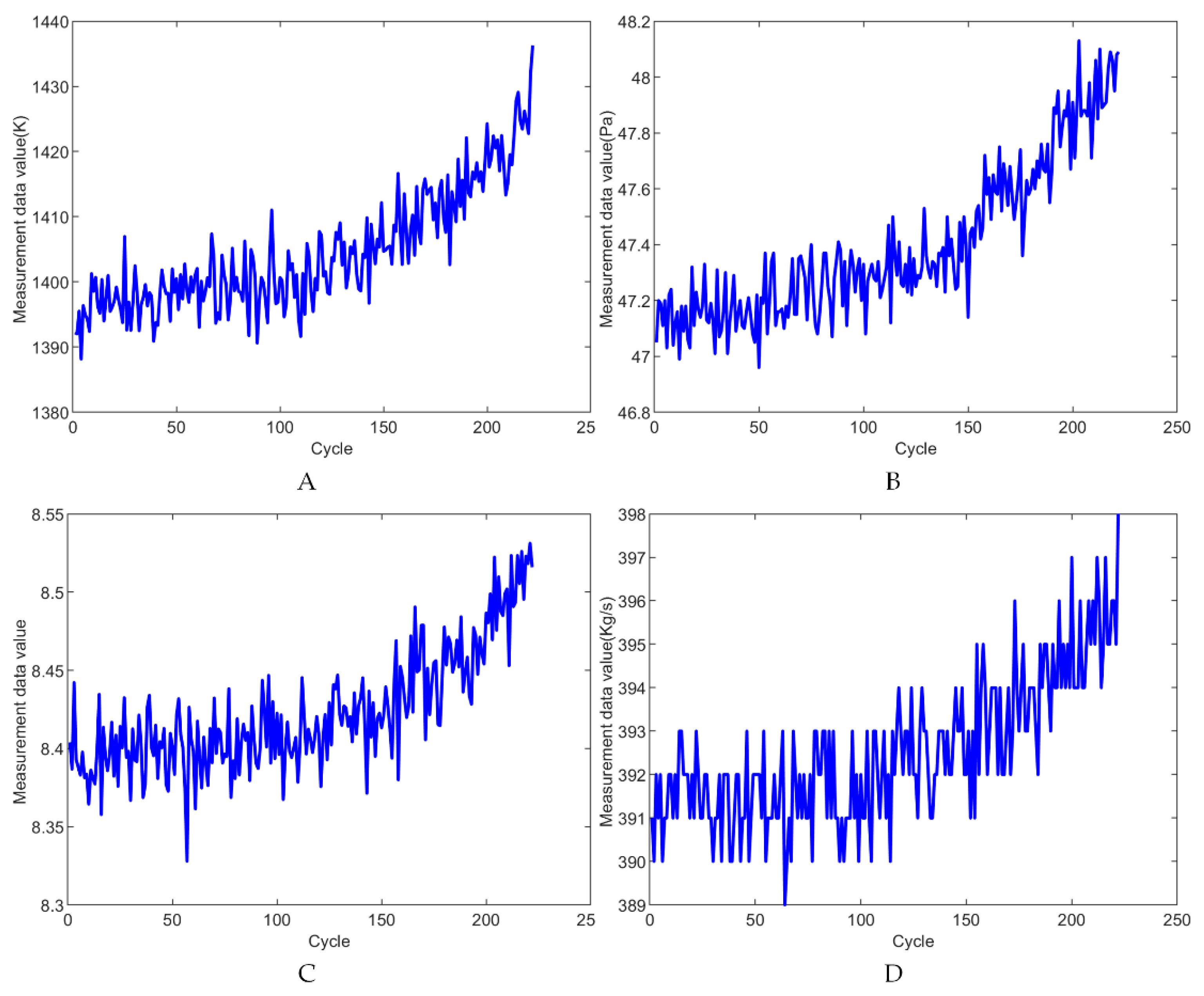
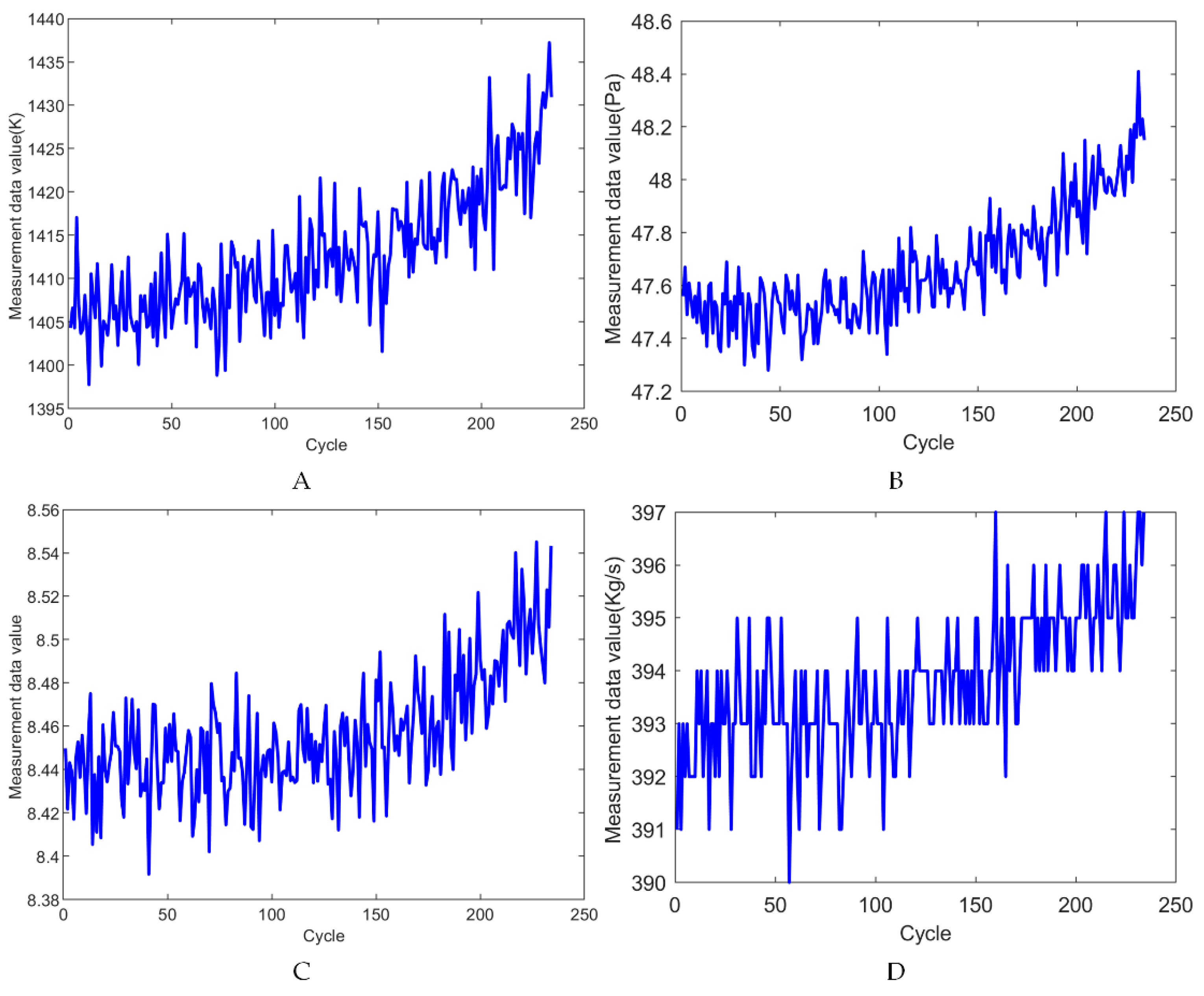
4.1. Dataset Description

To verify the applicability and effectiveness of the proposed multi-indicator degradation modeling and availability evaluation method, this study employs the Commercial Modular Aero-Propulsion System Simulation (C-MAPSS) dataset released by NASA as the experimental data source. Widely used in the field of aero-engine technical state management, this dataset contains operational and degradation data of multiple engines under varying conditions. It provides multivariate time-series sensor readings that can be used to construct degradation trajectories from multiple performance indicators. In this study, Subset FD001 is selected for modeling and analysis. This subset is characterized by a single operating condition, ensuring high consistency across samples and making it suitable for highlighting the model’s ability to capture inter-indicator coupling and reliability evolution.

The subset consists of data from 100 engine units, each recording time-series data from 21 sensors along with three operational settings.

Table 1. Description of the operational status and sensor information of the C-MAPSS experimental dataset.

Symbol	Meaning	Symbol	Meaning
H	Flight altitude	EPR	Engine compression ratio
Ma	Mach number	PS30	High-pressure compressor outlet static pressure
TRA	Throttle lever angle	PHI	Fuel flow and P30 ratio
T2	Fan inlet temperature	NRF	Corrected fan speed
T24	Low-pressure compressor outlet temperature	NRC	Core engine corrected speed
T30	High-pressure compressor outlet temperature	BPR	Bypass ratio
T50	Low-pressure turbine outlet temperature	FARB	Combustion chamber gas ratio
P2	Fan inlet pressure	HT_BLEED	Bleed air enthalpy
P15	Total bypass pressure	NF_DMD	Fan speed command value
P30	High-pressure compressor outlet total pressure	PCNFR_DMD	Fan correction speed command value
NF	Uncorrected fan speed	W31	High-pressure turbine cooling air flow
NC	Uncorrected core speed	W32	Low-pressure turbine cooling air flow

provides a detailed description of the sensor channels and operating conditions. Notably, several sensor readings exhibit no observable variation throughout the monitoring period and are thus excluded from the analysis. To reduce computational complexity and eliminate redundant information, this study applies the Spearman rank correlation coefficient to select the four most representative sensor channels: T50, PS30, BPR, and HT_BLEED. Engines #10 and #20 are randomly selected for experimental analysis. The raw sensor measurements for Engine 10 and Engine 20 are illustrated in Figure 1 and Figure 2, respectively.

To further enhance the expressiveness of the features and improve modeling stability, the four selected sensor indicators are fused to form a robust composite degradation feature. In this fusion process, each sensor signal is first normalized, and then a weighted averaging approach is employed to construct a single degradation index curve, which serves as a unified representation of the engine’s overall technical state. As shown in Figure 3, the fused degradation indices for both Engine 10 and Engine 20 demonstrate a clear monotonic increasing trend throughout the operational life. The resulting curves are smooth with minimal fluctuation, indicating that the fusion strategy retains the core degradation information from individual sensors while significantly suppressing high-frequency noise. This characteristic makes the composite feature more consistent with the statistical behavior of physical degradation processes and provides a solid foundation for subsequent degradation modeling and reliability assessments.

4.2. Evaluation Index

Three evaluation metrics are employed to quantify the prediction performance of the proposed model, namely root mean square error (RMSE), mean absolute error (MAE), and cumulative relative accuracy (CRA).

$$RMSE=\sqrt{{\displaystyle \frac{1}{\mathrm{N}}}{\left(L_{true}-L_{pred}\right)}^2}$$

(28)

$$MAE={\displaystyle \frac{1}{\mathrm{N}}}\left|L_{true}-L_{pred}\right|$$

(29)

$$CRA={\displaystyle \frac{1}{\mathrm{N}}}{\displaystyle \sum _{i=1}^{N}1-}{\displaystyle \frac{\left|L_{true,i}-L_{pred,i}\right|}{L_{true,i}}}$$

(30)

4.3. Construction of Predictive Models

To verify the effectiveness of the constructed Wiener process model in RUL prediction and reliability assessments, the model parameters estimated using the method described in Section 2.3 were applied to the composite state data of the engines. Based on these, the PDF, CDF, and reliability function of RUL were calculated. As illustrated in Figure 4 and Figure 5, the PDF exhibits a skewed distribution with a clear unimodal characteristic, indicating that the model provides a highly concentrated RUL prediction with good distributional consistency. The CDF increases over time, reflecting the rising cumulative probability that the engine will reach the failure threshold, consistent with the physical behavior of degrading systems. The reliability function decreases monotonically with time, capturing the continuous accumulation of failure risk during operation, which further validates the model’s capability to characterize degradation uncertainty.

To more clearly evaluate the effectiveness of different prediction methods, redundancy experiments were conducted using the T50 and PS30 sensor data. The comparison results are shown in

Table 2. Comparison of prediction results of different methods.

Dataset	Evaluation Index	C1	C2	C3
Engine 10	RMSE	36.6931	21.7358	2.2693
	MAE	36.6931	21.7358	2.2693
	CRA	−0.3724	0.0356	0.9897
Engine 20	RMSE	46.7134	35.2351	12.7846
	MAE	46.7134	35.2351	12.7846
	CRA	−0.2445	0.3925	0.9422

. Specifically, methods C1 and C2 represent single-stage degradation models applied to the T50 and PS30 data, respectively, but differ in the choice of trend functions. Method C1 adopts a linear degradation model, method C2 uses a power-law function, and method C3 applies an exponential function.

4.4. Optimization of Maintenance Strategies

Assuming that the daily maintenance cost of an aircraft engine is 20,000, the cost of preventive maintenance is 50,000, and the cost of corrective maintenance is 100,000. The average time for preventive maintenance is 10 cycles, and for corrective maintenance, 40 cycles. By substituting these parameters into Equations (21) and (25), the following results are obtained.

$$\begin{array}{cc}\hfill C\left(t\right)& ={\displaystyle \frac{20000+R\left(t,x\left(t\right)\right)50000+\left[1-R\left(t,x\left(t\right)\right)\right]100000}{{\displaystyle {\int }_{-\infty }^{t}R\left(t,x\left(t\right)\right)dt}}}\hfill \\ & ={\displaystyle \frac{120000-R\left(t,x\left(t\right)\right)50000}{{\displaystyle {\int }_{-\infty }^{t}R\left(t,x\left(t\right)\right)dt}}}\hfill \end{array}$$

(31)

$$\rho \left(t\right)={\displaystyle \frac{40-30R\left(t\right)}{{\displaystyle {\int }_{-\infty }^{t}R\left(t\right)}dt}}$$

(32)

As shown in Figure 6, the unit maintenance cost and availability under different monitoring intervals are presented. Figure 6A,B show the cost and availability curves for Engine 10, while Figure 6C,D correspond to Engine 20. It can be observed that with increasing monitoring intervals, the unit maintenance cost generally decreases, whereas availability rises rapidly before stabilizing. However, the optimal points for cost and availability do not align. For Engine 10, under the criterion of minimizing the unit maintenance cost, the optimal point occurs at the 193rd cycle, where the cost reaches its minimum at 507.4490, and the corresponding availability peaks at 0.5981, as shown the red circles in Figure 6A. Under the criterion of maximizing availability, the optimal point occurs at the 138th cycle, with the maximum availability reaching 0.9826 and the associated maintenance cost at 552.1942, as shown the red circles in Figure 6B. For Engine 20, the minimum unit maintenance cost is achieved at the 209th cycle, at 487.0936, with an availability of 0.3062, as shown the red circles in Figure 6C. When maximizing availability, the optimal cycle is the 144th, where the availability reaches 0.9831 and the associated maintenance cost is 532.9008, as shown the red circles in Figure 6D.

According to the optimization approach proposed in Section 2.3, to reasonably balance maintenance cost and availability, the maintenance cost is transformed into a negative value, thereby converting the problem into a unified single-objective optimization task. The results show that for Engine 10, the optimal maintenance cycle is 194. Compared to the solution focused solely on maximizing availability, the unit maintenance cost is reduced by 44.7452, while the availability remains high at 0.9801. For Engine 20, the optimal maintenance cycle is 209, yielding an availability of 0.9805 and a cost reduction of 65.0988 RMB compared to the availability-maximizing scenario.

These results demonstrate that the proposed method not only reduces computational complexity but also effectively achieves a trade-off between economic efficiency and system reliability. Compared with traditional single-objective optimization strategies, the proposed approach offers stronger practicality and engineering applicability, providing a more rational basis for maintenance decision-making regarding complex equipment.

5. Conclusions

This study addresses the decoupling problem between traditional RUL prediction and maintenance strategies by proposing a stochastic modeling-based maintenance optimization method that integrates multi-source degradation information. A composite degradation indicator was constructed from multi-sensor degradation signals, and a linear Wiener process model was employed to characterize the degradation behavior of the system. The corresponding reliability function, RUL distribution function, and availability expression were then derived, thereby incorporating both safety and economic factors into a unified optimization framework. The proposed method was validated using the NASA C-MAPSS aircraft engine dataset. Representative sensor variables were selected to construct the fused degradation features. Separate strategies were developed for maximizing availability and minimizing maintenance cost, and a joint optimization method was further applied to seek the optimal trade-off between the two objectives. The experimental results show that the proposed approach not only significantly reduces maintenance costs under the premise of maintaining high system reliability, but also effectively mitigates the conflict between maintenance objectives. This demonstrates strong engineering applicability and potential for broader deployment.

Despite the promising performance demonstrated in both simulation and real-world datasets, areas for further improvement remain. Currently, the degradation modeling is based on a linear Wiener process. Future work could incorporate nonlinear or state-dependent drift models to enhance the capability of capturing more complex degradation behaviors. The proposed methodology was validated on the C-MAPSS benchmark dataset, which, while widely recognized and realistic, does not fully capture all complexities of real-world industrial environments. Future work could extend the approach to proprietary or more diverse datasets to further assess its applicability. Second, the model assumes that sensor measurements and degradation processes follow specific statistical assumptions, which may not hold under all operational conditions. Additionally, the maintenance optimization considered cost and availability objectives, but other factors such as risk, resilience, and sustainability could also be incorporated into a more comprehensive decision-making framework. These findings have important implications for predictive maintenance practices.

References

1. Ren, W.; Wang, Z.; Chen, Z.; Zhao, S.; Dong, L.; Li, Y.; Fan, X. Multi-fault Feature Wasserstein Generative Adversarial Networks for Fault Diagnosis in Unbalanced Data. IEEE Trans. Instrum. Meas. 2025, 74, 3544909. [Google Scholar] [CrossRef]
2. Li, H.; Zhang, Z.; Li, T.; Si, X. A review on physics-informed data-driven remaining useful life prediction: Challenges and opportunities. Mech. Syst. Signal Process. 2024, 209, 111120. [Google Scholar] [CrossRef]
3. Broek, M.A.U.H.; Teunter, R.H.; de Jonge, B.; Veldman, J. Joint condition-based maintenance and condition-based production optimization. Reliab. Eng. Syst. Saf. 2021, 214, 107743. [Google Scholar] [CrossRef]
4. Jiménez, J.J.M.; Vingerhoeds, R.; Grabot, B.; Schwartz, S. An ontology model for maintenance strategy selection and assessment. J. Intell. Manuf. 2023, 34, 1369–1387. [Google Scholar] [CrossRef]
5. Lei, Y.; Li, N.; Guo, L.; Li, N.; Yan, T.; Lin, J. Machinery health prognostics: A systematic review from data acquisition to RUL prediction. Mech. Syst. Signal Process. 2018, 104, 799–834. [Google Scholar] [CrossRef]
6. Ali, A.; Abdelhadi, A. Condition-Based Monitoring and Maintenance: State of the Art Review. Appl. Sci. 2022, 12, 688. [Google Scholar] [CrossRef]
7. Ma, H.-G.; Wu, J.-P.; Li, X.-Y.; Kang, R. Condition-Based Maintenance Optimization for Multicomponent Systems Under Imperfect Repair—Based on RFAD Model. IEEE Trans. Fuzzy Syst. 2019, 27, 917–927. [Google Scholar] [CrossRef]
8. West, J.; Siddhpura, M.; Evangelista, A.; Haddad, A. Improving Equipment Maintenance—Switching from Corrective to Preventative Maintenance Strategies. Buildings 2024, 14, 3581. [Google Scholar] [CrossRef]
9. Cao, Y.; Luo, J.; Dong, W. Optimization of condition-based maintenance for multi-state deterioration systems under random shock. Appl. Math. Model. 2023, 115, 80–99. [Google Scholar] [CrossRef]
10. Chen, N.; Ye, Z.-S.; Xiang, Y.; Zhang, L. Condition-based maintenance using the inverse Gaussian degradation model. Eur. J. Oper. Res. 2015, 243, 190–199. [Google Scholar] [CrossRef]
11. Zhao, X.; Fouladirad, M.; Bérenguer, C.; Bordes, L. Condition-based inspection/replacement policies for non-monotone deteriorating systems with environmental covariates. Reliab. Eng. Syst. Saf. 2010, 95, 921–934. [Google Scholar] [CrossRef]
12. You, M.Y. A generalized three-type lifetime probabilistic models-based hybrid maintenance policy with a practical switcher for time-based preventive maintenance and condition-based maintenance. Proc. Inst. Mech. Eng. Part E J. Process Mech. Eng. 2019, 233, 1231–1244. [Google Scholar] [CrossRef]
13. Arts, J.; Basten, R. Design of multi-component periodic maintenance programs with single-component models. IISE Trans. 2018, 50, 606–615. [Google Scholar] [CrossRef]
14. Ding, S.H.; Kamaruddin, S.; Azid, I.A. Development of a model for optimal maintenance policy selection. Eur. J. Ind. Eng. 2014, 8, 50–68. [Google Scholar] [CrossRef]
15. Zhu, Z.; Xiang, Y.; Li, M.; Zhu, W.; Schneider, K. Preventive maintenance subject to equipment unavailability. IEEE Trans. Reliab. 2019, 68, 1009–1020. [Google Scholar] [CrossRef]
16. Wang, Z.; Jiang, P.; Chen, Z.; Li, Y.; Ren, W.; Dong, L.; Du, W.; Wang, J.; Zhang, X.; Shi, H. Remaining useful life prediction method based on two-phase adaptive drift Wiener process. Reliab. Eng. Syst. Saf. 2025, 258, 110908. [Google Scholar] [CrossRef]
17. Jiang, P.; Ren, W.; Chen, Z.; Wang, Z.; Li, Y.; Dong, L. A nonlinear dynamic ensemble remaining useful life prediction method considering multi-source data uncertainty. Mech. Syst. Signal Process. 2025, 230, 112607. [Google Scholar] [CrossRef]
18. Wang, F.; Ni, X.; Zhang, Q.; Guo, S.; Zhou, J.; Chen, D. Estimation of combine harvester throughput using multisensor data fusion. Comput. Electron. Agric. 2025, 237, 110713. [Google Scholar] [CrossRef]
19. Gu, M. Improved kalman filtering and adaptive weighted fusion algorithms for enhanced multi-sensor data fusion in precision measurement. Informatica 2025, 49, 85–100. [Google Scholar] [CrossRef]
20. Khemani, K. AI-Driven Predictive Maintenance with Real-Time Contextual Data Fusion for Connected Vehicles. Res. Sq. 2025; in press. [Google Scholar] [CrossRef]
21. Orošnjak, M. Enhancing sustainability in tyre manufacturing with machine learning and knowledge graphs: An energy-based maintenance solution. J. Clean. Prod. 2025, 520, 146090. [Google Scholar] [CrossRef]
22. Zhang, J.-X.; Hu, C.-H.; He, X.; Si, X.-S.; Liu, Y.; Zhou, D.-H. A Novel Lifetime Estimation Method for Two-Phase Degrading Systems. IEEE Trans. Reliab. 2019, 68, 689–709. [Google Scholar] [CrossRef]
Figure 1. The measurement data of Engine 10: (A) is T50; (B) is PS30; (C) is BPR; (D) is HT_BLEED.
Machines 13 00633 g001
Figure 2. The measurement data of Engine 20: (A) is T50; (B) is PS30; (C) is BPR; (D) is HT_BLEED.
Machines 13 00633 g002
Figure 3. The composite status index of engines 10 and 20. (A) is engine 10; (B) is engine 20.
Machines 13 00633 g003
Figure 4. RUL prediction results for Engine 10: (A) PDF of the remaining lifetime; (B) CDF of the remaining lifetime; (C) CDF of the remaining lifetime.
Machines 13 00633 g004
Figure 5. RUL prediction results for Engine 20: (A) PDF of the remaining lifetime; (B) CDF of the remaining lifetime; (C) CDF of the remaining lifetime.
Machines 13 00633 g005
Figure 6. Maintenance cost and availability for the FD001 dataset: (A) Maintenance cost of engine 10; (B) Availability of Engine 10; (C) Maintenance cost of engine 20; (D) Availability of Engine 20.
Machines 13 00633 g006