
Effects of Vibration Direction, Feature Selection, and the SVM Kernel on Unbalance Fault Classification


Abstract
1. Introduction
2. Materials and Methods
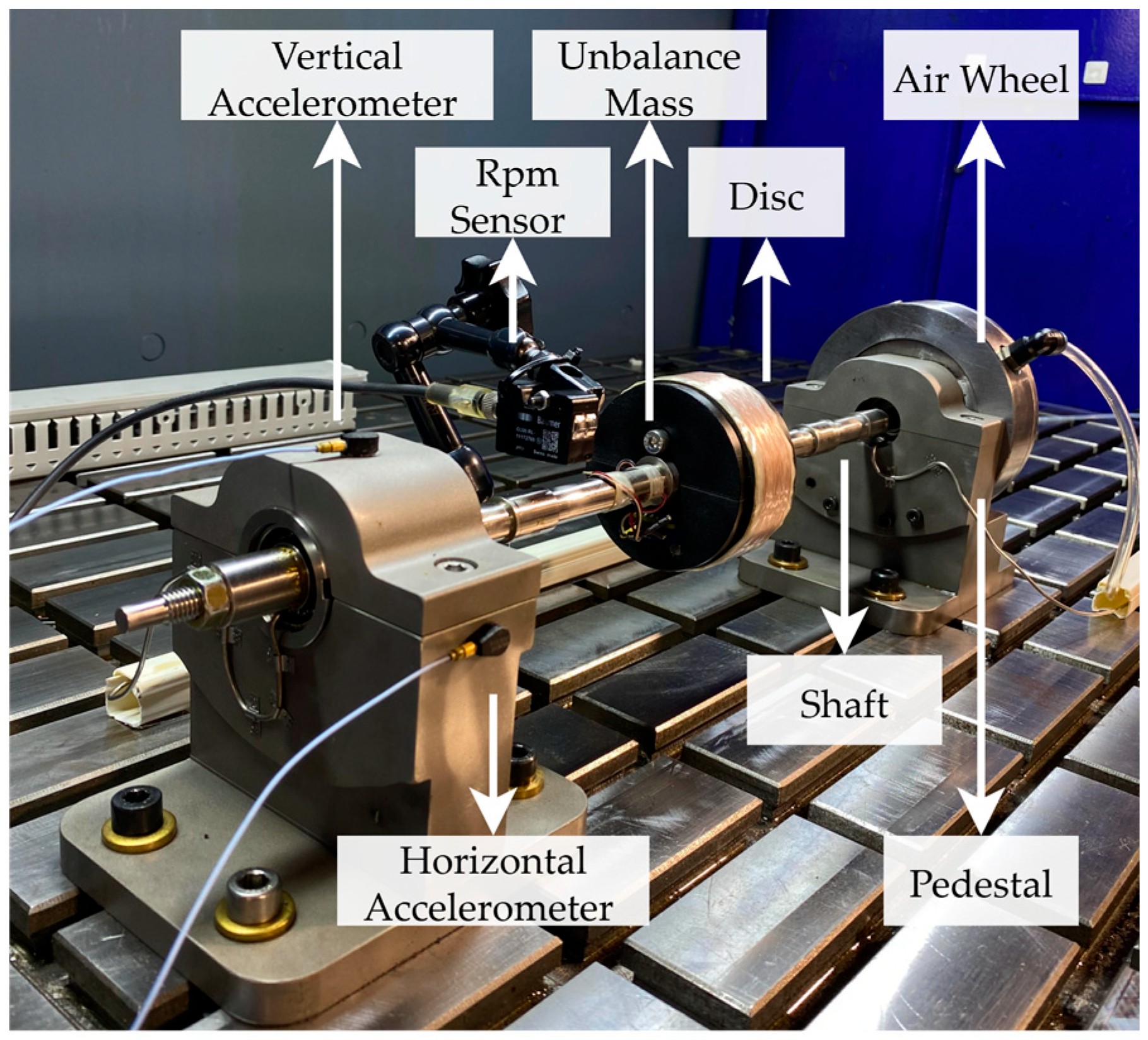
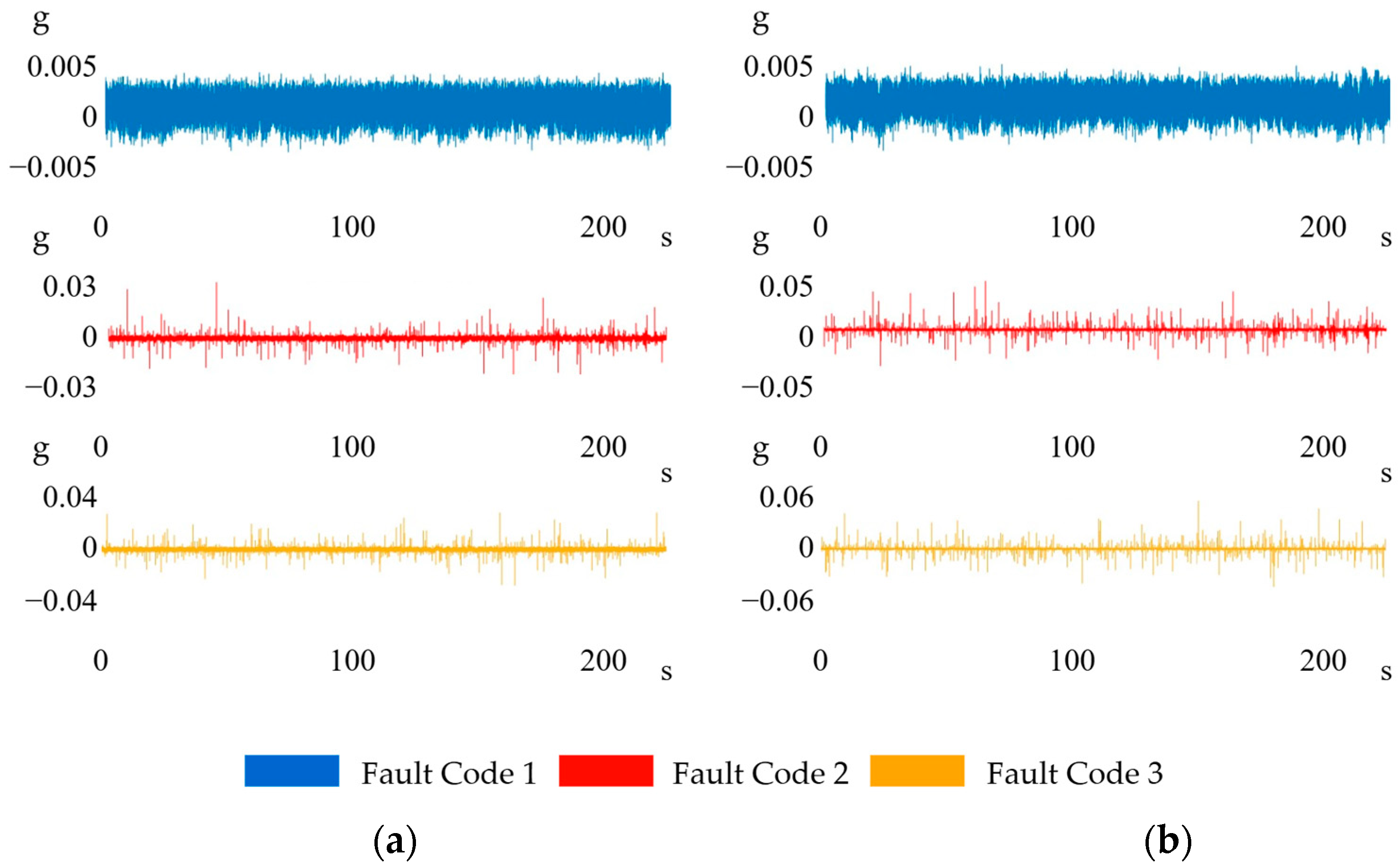
2.1. Experimental Setup
2.2. Feature Extraction
2.2.1. Time Domain Analysis and Temporal Features
2.2.2. Frequency Domain Analysis and Spectral Features
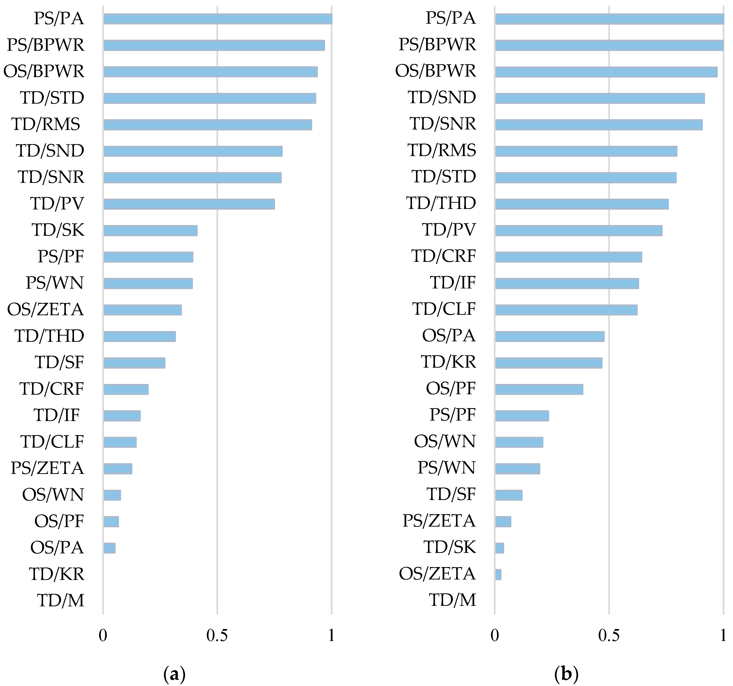
2.3. Feature Ranking
2.4. K-Fold Cross-Validation
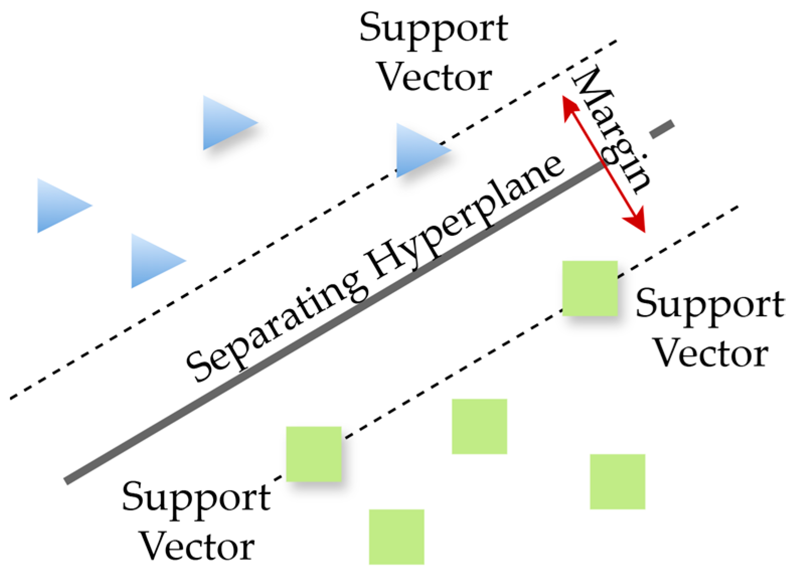
2.5. Classification
3. Results and Discussion
4. Conclusions
Author Contributions
Funding
Data Availability Statement
Conflicts of Interest
Abbreviations
| c | Damping coefficient |
| D | Distortion power |
| k | Stiffness |
| m | Mass |
| N | Noise power |
| S | Signal power |
References
- Almutairi, K.; Sinha, J.K.; Wen, H. Fault detection of rotating machines using poly-coherent composite spectrum of measured vibration responses with machine learning. Machines 2024, 12, 573. [Google Scholar] [CrossRef]
- Singh, S.; Kumar, N. Rotor faults diagnosis using artificial neural networks and support vector machines. Int. J. Acoust. Vib. 2015, 20, 153–159. [Google Scholar] [CrossRef]
- Tahir, M.M.; Hussain, A.; Badshah, S.; Khan, A.Q.; Iqbal, N. Classification of unbalance and misalignment faults in rotor using multi-axis time domain features. In Proceedings of the 2016 International Conference on Emerging Technologies (ICET), Islamabad, Pakistan, 16 January 2017; pp. 1–4. [Google Scholar] [CrossRef]
- Bechiri, M.B.; Allal, A.; Naoui, M.; Khechekhouche, A.; Alsaif, H.; Boudjemline, A. Effective diagnosis approach for broken rotor bar fault using bayesian-based optimization of machine learning hyperparameters. IEEE Access 2024, 12, 3464108. [Google Scholar] [CrossRef]
- Ozkat, E.C. Vibration data-driven anomaly detection in UAVs: A deep learning approach. Eng. Sci. Technol. Int. J. 2024, 54, 101702. [Google Scholar] [CrossRef]
- Akyaz, T.; Engın, D. Machine learning-based predictive maintenance system for artificial yarn machines. IEEE Access 2024, 12, 125446–125461. [Google Scholar] [CrossRef]
- Zhu, T.; Ran, Y.; Zhou, X.; Wen, Y. A survey of predictive maintenance: Systems, purposes and approaches. arXiv 2019, arXiv:1912.07383. [Google Scholar] [CrossRef]
- Lan, L.; Liu, X.; Wang, Q. Fault detection and classification of the rotor unbalance based on dynamics features and support vector machine. Meas. Control 2023, 56, 1075–1086. [Google Scholar] [CrossRef]
- Zhang, J.; Ma, W.; Lin, J.; Ma, L.; Jia, X. Fault diagnosis approach for rotating machinery based on dynamic model and computational intelligence. Measurement 2015, 59, 73–87. [Google Scholar] [CrossRef]
- Hübner, G.R.; Pinheiro, H.; de Souza, C.E.; Franchi, C.M.; da Rosa, L.D.; Dias, J.P. Detection of mass imbalance in the rotor of wind turbines using Support Vector Machine. Renew. Energy 2021, 170, 49–59. [Google Scholar] [CrossRef]
- Nti, I.K.; Nyarko-Boateng, O.; Aning, J. Performance of machine learning algorithms with different k values in k-fold cross validation. Int. J. Inf. Technol. Comput. Sci. 2021, 13, 61–71. [Google Scholar] [CrossRef]
- Nath, A.G.; Udmale, S.S.; Singh, S.K. Role of artificial intelligence in rotor fault diagnosis: A comprehensive review. Artif. Intell. Rev. 2021, 54, 2609–2668. [Google Scholar] [CrossRef]
- Alsaleh, A.; Sedighi, H.M.; Ouakad, H.M. Experimental and theoretical investigations of the lateral vibrations of an unbalanced Jeffcott rotor. Front. Struct. Civ. Eng. 2020, 14, 1024–1032. [Google Scholar] [CrossRef]
- Jamil, M.A.; Khanam, S. Influence of One-Way ANOVA and Kruskal–Wallis based feature ranking on the performance of ML classifiers for bearing fault diagnosis. J. Vib. Eng. Technol. 2024, 12, 3101–3132. [Google Scholar] [CrossRef]
- McKight, P.E.; Najab, J. Kruskal-wallis test. In The Corsini Encyclopedia of Psychology; Wiley Online Library: Hoboken, NJ, USA, 2010; p. 1. [Google Scholar] [CrossRef]
- ISO 21940-11; Mechanical vibration—Rotor balancing—Part 11: Procedures and tolerances for rotors with rigid behaviour. International Organization for Standardization (ISO): Geneva, Switzerland, 2016.
- Choudhury, T.; Viitala, R.; Kurvinen, E.; Viitala, R.; Sopanen, J. Unbalance estimation for a large flexible rotor using force and displacement minimization. Machines 2020, 8, 39. [Google Scholar] [CrossRef]
- Girdhar, P.; Scheffer, C. Practical Machinery Vibration Analysis and Predictive Maintenance, 1st ed.; Elsevier: Oxford, England, 2004; p. 90. [Google Scholar] [CrossRef]
- Wang, C.; Sun, H.; Cao, X. Construction of the efficient attention prototypical net based on the time–frequency characterization of vibration signals under noisy small sample. Measurement 2021, 179, 109412. [Google Scholar] [CrossRef]
- Xiang, B.; Xu, J.; Liu, Z.; Wong, W.; Zheng, L. Vibration characteristics and cross-feedback control of magnetically suspended blower based on complex-factor model. J. Sound Vib. 2023, 556, 117729. [Google Scholar] [CrossRef]
- Kasdin, N.J.; Paley, D.A. Engineering Dynamics: A Comprehensive Introduction, 1st ed.; Princeton University Press: Princeton, NJ, USA, 2011; p. 489. [Google Scholar]
- El Badaoui, M.; Bonnardot, F. Impact of the non-uniform angular sampling on mechanical signals. Mech. Syst. Signal Process. 2014, 44, 199–210. [Google Scholar] [CrossRef]
- Leis, J.W. Digital Signal Processing Using MATLAB for Students and Researchers, 1st ed.; Wiley: Hoboken, NJ, USA, 2011; pp. 81–82. [Google Scholar] [CrossRef]
- Hendrickx, K.; Meert, W.; Mollet, Y.; Gyselinck, J.; Cornelis, B.; Gryllias, K.; Davis, J. A general anomaly detection framework for fleet-based condition monitoring of machines. Mech. Syst. Signal Process. 2020, 139, 106585. [Google Scholar] [CrossRef]
- Domingos, P. A few useful things to know about machine learning. Commun. ACM. 2012, 55, 78–87. [Google Scholar] [CrossRef]
- Lei, Y. Intelligent Fault Diagnosis and Remaining Useful Life Prediction of Rotating Machinery, 1st ed.; Elsevier: Amsterdam, The Netherlands, 2017; pp. 30–38, 121–124. [Google Scholar] [CrossRef]
- Vishwakarma, M.; Purohit, R.; Harshlata, V.; Rajput, P. Vibration analysis & condition monitoring for rotating machines: A review. Mater. Today Proc. 2017, 4, 2659–2664. [Google Scholar] [CrossRef]
- MathWorks. Predictive Maintenance Toolbox™ User’s Guide, R2021b; MathWorks Inc.: Natick, MA, USA, 2021; Available online: https://www.mathworks.com/help/predmaint/ (accessed on 21 July 2025).
- Kester, W. MT-003 TUTORIAL Understand SINAD, ENOB, SNR, THD, THD + N, and SFDR so You Don’t Get Lost in the Noise Floor; Analog Devices: Norwood, MA, USA, 2009. [Google Scholar]
- Vargas-Lopez, O.; Perez-Ramirez, C.A.; Valtierra-Rodriguez, M.; Yanez-Borjas, J.J.; Amezquita-Sanchez, J.P. An explainable machine learning approach based on statistical indexes and svm for stress detection in automobile drivers using electromyographic signals. Sensors 2021, 21, 3155. [Google Scholar] [CrossRef] [PubMed]
- Hassan, S.; Li, Q.; Zubair, M.; Alsowail, R.A.; Qureshi, M.A. Unveiling the correlation between nonfunctional requirements and sustainable environmental factors using a machine learning model. Sustainability 2024, 16, 5901. [Google Scholar] [CrossRef]
- Pule, M.; Matsebe, O.; Samikannu, R. Application of PCA and SVM in fault detection and diagnosis of bearings with varying speed. Math. Probl. Eng. 2022, 2022, 5266054. [Google Scholar] [CrossRef]
- Vamsi, I.; Sabareesh, G.R.; Penumakala, P.K. Comparison of condition monitoring techniques in assessing fault severity for a wind turbine gearbox under non-stationary loading. Mech. Syst. Signal Process. 2019, 124, 1–20. [Google Scholar] [CrossRef]
- Hasan, M.M.; Chowdhury, D.; Hasan, A.S.M.K. Statistical features extraction and performance analysis of supervised classifiers for non-intrusive load monitoring. Eng. Lett. 2019, 27, 776–782. [Google Scholar]
- MathWorks. Statistics and Machine Learning Toolbox™ User’s Guide, R2016b; MathWorks Inc.: Natick, MA, USA, 2016; Available online: https://www.mathworks.com/help/stats/ (accessed on 21 July 2025).
- Al-Haddad, L.A.; Jaber, A.A.; Hamzah, M.N.; Fayad, M.A. Vibration-current data fusion and gradient boosting classifier for enhanced stator fault diagnosis in three-phase permanent magnet synchronous motors. Electr. Eng. 2023, 106, 3253–3268. [Google Scholar] [CrossRef]
- Tharwat, A. Classification assessment methods. Appl. Comput. Inform. 2020, 17, 168–192. [Google Scholar] [CrossRef]
- Kafeel, A.; Aziz, S.; Awais, M.; Khan, M.A.; Afaq, K.; Idris, S.A.; Alshazly, H.; Mostafa, S.M. An expert system for rotating machine fault detection using vibration signal analysis. Sensors 2021, 21, 7587. [Google Scholar] [CrossRef] [PubMed]


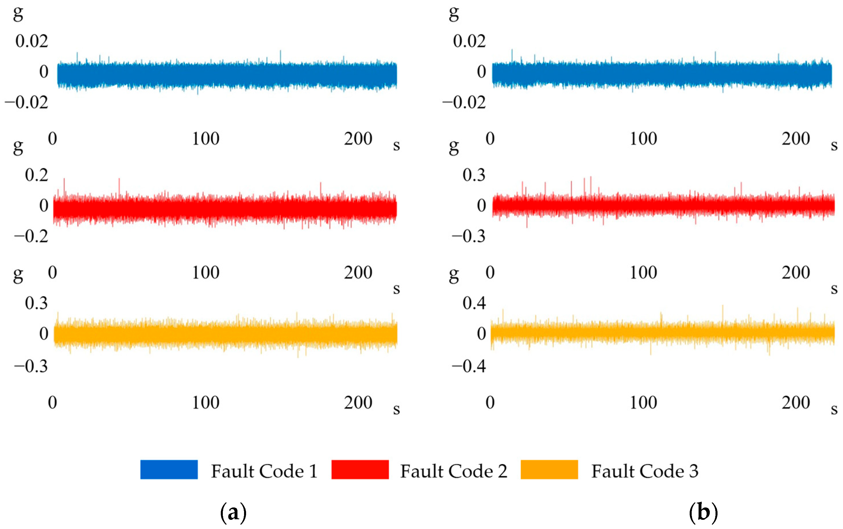
| Fault Code | Load Conditions | Number of Observations | Number of Samples in Each Observation | Duration of Each Observation |
|---|---|---|---|---|
| 1 | 0 g | 300 | 4096 | 1s |
| 2 | 3.6 g | 300 | 4096 | 1s |
| 3 | 5.2 g | 300 | 4096 | 1s |
| Time Domain | Frequency Domain | ||
|---|---|---|---|
| Signal Statics | Spectral Features | ||
| Feature | Acronym | Feature | Acronym |
| Mean | M | Band power | BPWR |
| Root mean square | RMS | Natural frequency | WN |
| Peak value | PV | Peak amplitude | PA |
| Signal-to-noise ratio | SNR | Damping factor | ZETA |
| Signal to noise and distortion ratio | SND | Peak frequency | PF |
| Total harmonic distortion | THD | ||
| Standard deviation | STD | ||
| Impulse factor | IF | ||
| Crest factor | CRF | ||
| Clearance factor | CLF | ||
| Shape factor | SF | ||
| Skewness | SK | ||
| Kurtosis | KR | ||
| Description | Equation | Description | Equation |
|---|---|---|---|
| M | CLF | ||
| RMS | SF | ||
| PV | SK | ||
| SNR | KR | ||
| SND | BPWR | ||
| THD | WN | ||
| STD | PA | ||
| IF | ZETA | ||
| CRF | PF |
| Kernel of SVM | Kernel Function | Kernel Scale |
|---|---|---|
| Linear | Linear | Auto |
| Quadratic | 2-order polynomial | Auto |
| Cubic | 3-order polynomial | Auto |
| Fine Gaussian | RBF | |
| Medium Gaussian | RBF | |
| Coarse Gaussian | RBF |
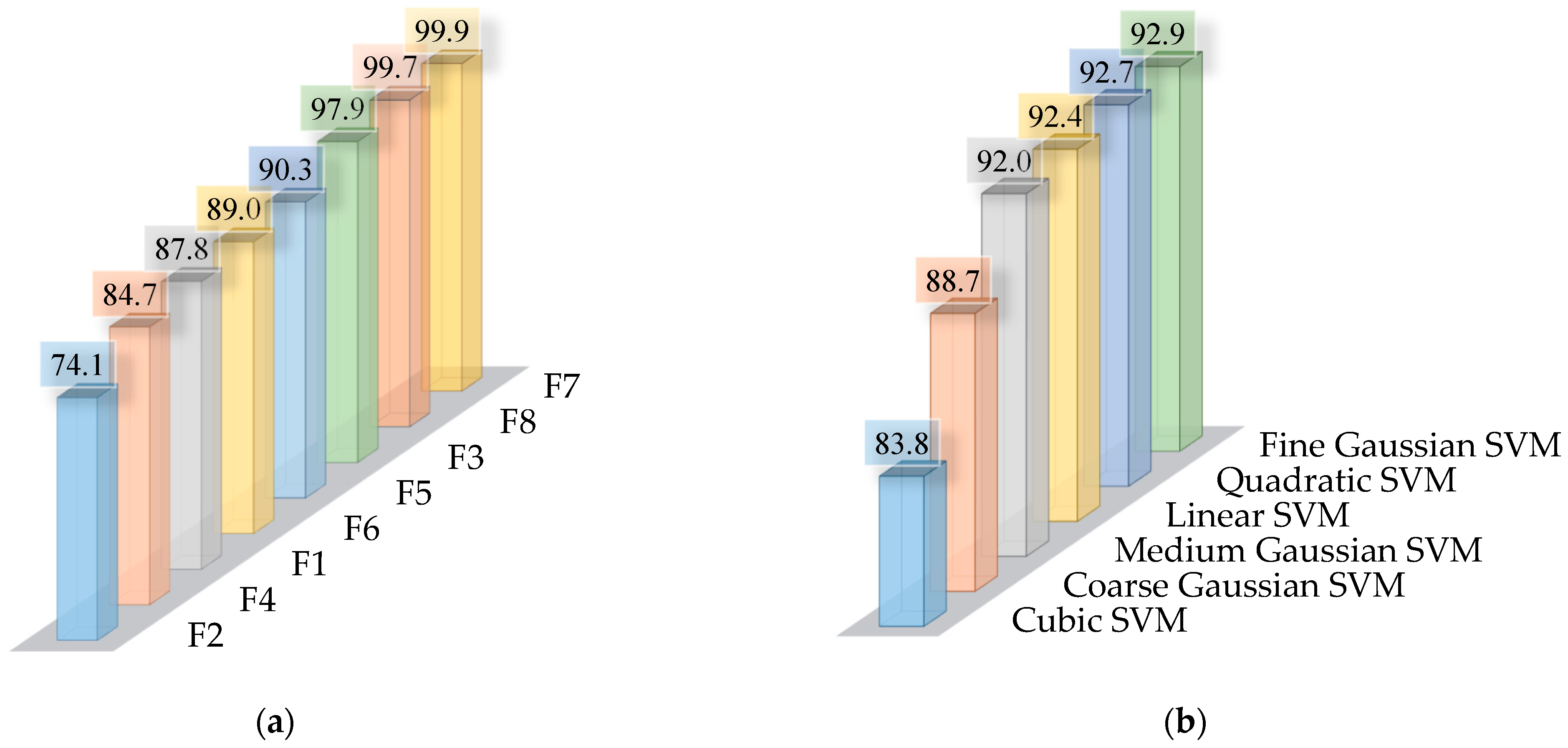
| Feature Set | Feature Domain | Measurement Axis | Selected Features |
|---|---|---|---|
| F1 | Time | Horizontal | STD, RMS, SND |
| F2 | Frequency–OS | Horizontal | BPWR, ZETA, WN |
| F3 | Frequency–PS | Horizontal | PA, BPWR, PF |
| F4 | Hybrid | Horizontal | All nine features |
| F5 | Time | Vertical | SND, SNR, RMS |
| F6 | Frequency–OS | Vertical | BPWR, PA, PF |
| F7 | Frequency–PS | Vertical | PA, BPWR, PF |
| F8 | Hybrid | Vertical | All nine features |
| Feature Set | Linear SVM (%) | Quadratic SVM (%) | Cubic SVM (%) | Fine Gaussian SVM (%) | Medium Gaussian SVM (%) | Coarse Gaussian SVM (%) |
|---|---|---|---|---|---|---|
| F1 | 90.1 | 90.0 | 76.0 | 90.3 | 90.6 | 89.6 |
| F2 | 77.3 | 79.4 | 60.0 | 79.9 | 78.2 | 69.7 |
| F3 | 97.9 | 97.7 | 98.1 | 97.7 | 98.0 | 98.0 |
| F4 | 85.0 | 84.9 | 85.0 | 83.4 | 85.0 | 84.9 |
| F5 | 90.9 | 93.1 | 76.7 | 94.3 | 93.8 | 92.9 |
| F6 | 97.8 | 97.3 | 74.7 | 98.4 | 90.6 | 75.2 |
| F7 | 100 | 99.7 | 100 | 99.9 | 100 | 100 |
| F8 | 100 | 99.8 | 99.9 | 99.0 | 99.9 | 99.6 |
| Analysis | Friedman χ2 (df) | p Value | Kendall’s W | Smallest Raw Wicoxon p | Smallest Holm Adjusted p |
|---|---|---|---|---|---|
| Kernels | 5.92 (5) | 0.314 | 0.148 | 0.041 | 0.416 |
| Feature sets | 37.59 (7) | <0.001 | 0.895 | 0.031 | 0.875 |
| Training Results | Linear SVM | Quadratic SVM | Cubic SVM | Fine Gaussian SVM | Medium Gaussian SVM | Coarse Gaussian SVM |
|---|---|---|---|---|---|---|
| Accuracy (%) | 100 | 99.7 | 100 | 99.9 | 100 | 100 |
| Total cost | 0 | 3 | 0 | 1 | 0 | 0 |
| Prediction speed (obs/s) | 9600 | 5600 | 4800 | 5000 | 9200 | 9000 |
| Training time (s) | 2.624 | 2.923 | 2.738 | 2.576 | 2.465 | 2.684 |
| Model size (compact) (kB) | 16 | 16 | 16 | 21 | 19 | 25 |
Disclaimer/Publisher’s Note: The statements, opinions and data contained in all publications are solely those of the individual author(s) and contributor(s) and not of MDPI and/or the editor(s). MDPI and/or the editor(s) disclaim responsibility for any injury to people or property resulting from any ideas, methods, instructions or products referred to in the content. |
© 2025 by the authors. Licensee MDPI, Basel, Switzerland. This article is an open access article distributed under the terms and conditions of the Creative Commons Attribution (CC BY) license (https://creativecommons.org/licenses/by/4.0/).
Share and Cite
Ateş, M.; Erkuş, B. Effects of Vibration Direction, Feature Selection, and the SVM Kernel on Unbalance Fault Classification. Machines 2025, 13, 634. https://doi.org/10.3390/machines13080634
Ateş M, Erkuş B. Effects of Vibration Direction, Feature Selection, and the SVM Kernel on Unbalance Fault Classification. Machines. 2025; 13(8):634. https://doi.org/10.3390/machines13080634
Chicago/Turabian StyleAteş, Mine, and Barış Erkuş. 2025. "Effects of Vibration Direction, Feature Selection, and the SVM Kernel on Unbalance Fault Classification" Machines 13, no. 8: 634. https://doi.org/10.3390/machines13080634
APA StyleAteş, M., & Erkuş, B. (2025). Effects of Vibration Direction, Feature Selection, and the SVM Kernel on Unbalance Fault Classification. Machines, 13(8), 634. https://doi.org/10.3390/machines13080634