Abstract
To address the obstacle-avoidance path-planning requirements of dual-arm robots operating in complex environments, such as chemical laboratories and biomedical workstations, this paper proposes ODSN-RRT (optimization-direction-step-node RRT), an efficient planner based on rapidly-exploring random trees (RRT). ODSN-RRT integrates three key optimization strategies. First, a two-stage sampling-direction strategy employs goal-directed growth until collision, followed by hybrid random-goal expansion. Second, a dynamic safety step-size strategy adapts each extension based on obstacle size and approach angle, enhancing collision detection reliability and search efficiency. Third, an expansion-node optimization strategy generates multiple candidates, selects the best by Euclidean distance to the goal, and employs backtracking to escape local minima, improving path quality while retaining probabilistic completeness. For collision checking in the dual-arm workspace (self and environment), a cylindrical-spherical bounding-volume model simplifies queries to line-line and line-sphere distance calculations, significantly lowering computational overhead. Redundant waypoints are pruned using adaptive segmental interpolation for smoother trajectories. Finally, a master-slave planning scheme decomposes the 14-DOF problem into two 7-DOF sub-problems. Simulations and experiments demonstrate that ODSN-RRT rapidly generates collision-free, high-quality trajectories, confirming its effectiveness and practical applicability.
1. Introduction
Compared with single-arm robots, dual-arm robots feature a larger workspace, higher payload capacity, and coordinated bimanual actions, which have driven their rapid development and widespread deployment in industrial manufacturing, aerospace, medical rehabilitation, and other domains [1,2,3,4]. Within intelligent-manufacturing settings, their kinematic redundancy and operational flexibility render them indispensable for laboratory tasks such as sample preparation, transportation of reagent tubes and microtiter plates, liquid transfer, and hazardous-materials handling [5,6,7]. However, the spatial compactness and cluttered obstacle distribution typical of chemical laboratory environments require dual-arm robots to avoid both environmental collisions and self-collisions, thereby considerably increasing the complexity of motion planning and the associated computational cost [8,9].
To this end, researchers worldwide have proposed a broad spectrum of robot motion-planning strategies [10], which can be broadly classified into graph-search-based algorithms [11], sampling-based algorithms [12], and intelligent meta-heuristic algorithms [13]. Representative techniques include the artificial potential field (APF) method [14], the A* algorithm [15], particle swarm optimization (PSO) [16], the probabilistic roadmap (PRM) [17], and rapidly-exploring random trees (RRTs) [18]. The APF approach is efficient for global path construction, yet it is prone to local-minimum entrapment. A* performs well in low-dimensional search spaces; however, its exponential memory demand for storing the entire search space restricts its applicability to high-degree-of-freedom robotic manipulators.
Sampling-based planning methods have become indispensable tools for motion planning in high-degree-of-freedom (DoF) robotic systems. Among them, the rapidly-exploring random tree (RRT) algorithm proposed by LaValle has been widely adopted because of its probabilistic completeness and its ability to efficiently explore continuous state spaces. The RRT is a single-query planner that incrementally builds a search tree through random sampling in multi-dimensional configuration spaces, making it particularly effective in environments containing numerous static and dynamic obstacles. However, the conventional RRT suffers from low sampling efficiency, an abundance of redundant nodes, and sub-optimal path quality [19,20]. Consequently, a variety of enhanced variants have been proposed to address these shortcomings.
Kang et al. [21] proposed the EDDS-bi-RRT algorithm for multi-DoF dual-arm manipulators; by introducing cosine–sine perturbations for adaptive direction sampling and mapping the step size to the minimum safety clearance within a bidirectional RRT framework, they markedly accelerated convergence in unstructured environments. Jiang et al. [22] combined Gaussian-constrained random sampling with an artificial potential field to guide tree expansion, but their approach remains susceptible to local minima. Daniel and André [23] introduced AM-RRT*, the first method to embed diffusion distance into nearest-neighbor retrieval and to employ informed-sampling reconnection, thereby compressing the search tree in high-dimensional spaces and improving both convergence speed and path quality. Shi et al. [24] enhanced RRT with goal-bias sampling and node-cost selection, effectively reducing fruitless expansions and achieving higher planning success rates. Dong et al. [25] developed an improved RRT within a master–slave framework for dual-arm collaboration; their design incorporates a distance–joint-variance weighted cost function, a time-window sphere collision model, and interpolation smoothing to enhance trajectory continuity. Wang et al. [26] proposed a hybrid APF-RRT* scheme for disinfection robots that leverages a virtual potential field and a fuzzy adaptive step size to generate shorter and safer routes in cluttered environments. Wang et al. [27] introduced GMR-RRT*, a sampling-based planner that embeds Gaussian mixture regression (GMR) into the RRT* sampling process to learn from human demonstration trajectories. By bootstrapping non-uniform samples according to the learned GMR model, GMR-RRT* achieves significantly faster convergence and higher-quality paths than classical RRT* planners. Addressing the RRT’s notorious inefficiency and proliferation of redundant nodes, Fang et al. [28] proposed G-RRT, which integrates a goal-bias strategy, dynamic step-size extension, and a tree-pruning mechanism. Together, these enhancements markedly improve search efficiency and path quality in robotic-arm obstacle-avoidance scenarios. Despite these advances, RRT and its derivatives (e.g., RRT* [29], Informed-RRT* [30], BIT* [31]) still impose substantial computational burdens when applied to complex dual-arm robotic systems.
Obstacle-avoidance motion planning is pivotal to the safe and efficient execution of coordinated tasks by dual-arm robots. To mitigate the sampling inefficiency, local-trap stagnation, and heavy collision-checking overhead inherent in conventional RRT, this study introduces the ODSN-RRT (optimization–direction–step–node RRT) algorithm. By collaboratively optimizing the sampling direction, dynamic step size, and expansion-node selection in conjunction with a geometry-based collision-detection framework and a master–slave planning scheme, ODSN-RRT delivers high-efficiency path planning for dual-arm manipulators. The principal contributions are as follows:
- Two-stage sampling-direction strategy. Stage I performs greedy growth toward the goal. Upon collision, Stage II engages a hybrid expansion strategy that combines goal bias with random perturbations to steer the tree. This preserves both exploration and exploitation, enabling efficient discovery of feasible paths.
- Dynamic safety step-size strategy. The expansion step is adaptively scaled according to the obstacle’s minimum enclosing diameter and the approach angle, maintaining collision-checking validity and accelerating search in cluttered environments.
- Expansion-node optimization with backtracking recovery. Multiple candidate nodes are generated and evaluated to select the optimal expansion point. A failure backtracking mechanism resets the search to a parent node after consecutive dead ends, improving node quality and preventing stagnation in local traps.
- Cylindrical–spherical collision-detection framework. A unified geometric model streamlines both self-collision and environmental collision computations for dual-arm systems.
- Path optimization and master–slave planning. Segment-wise collision checking prunes redundant nodes, while a master–slave scheme decouples the two arms, enhancing cooperative feasibility and curbing the computational load in high-dimensional spaces.
The proposed method has been validated through Python and MATLAB simulations, as well as extensive experiments on a physical dual-arm robotic platform, demonstrating superior efficiency and path quality. Furthermore, ODSN-RRT provides both theoretical insights and practical solutions for obstacle-avoidance path planning in high-degree-of-freedom robotic systems.
2. Kinematic Modelling
This paper is based on the laboratory-owned Diana7 platform of the Agile dual-arm robot, which mainly consists of a body base and two seven-degree-of-freedom robotic arms. Figure 1a illustrates the constructed 3-D model of the Agile dual-arm robot, where one arm serves as the master arm and the other as the slave arm. Subsequently, the kinematic model of the dual arms is developed according to the improved Denavit–Hartenberg (D–H) convention, which attaches a reference frame to each link of the manipulator, with the coordinate system of the D–H parameters of the master arm presented in Figure 1b. The D–H parameters of the robot are detailed in Table 1. Furthermore, the joint diagrams of the slave and master arms are mirror-symmetrical to the robot body, resulting in the D–H parameters α and θ of the master arm being opposite to those of the slave arm.
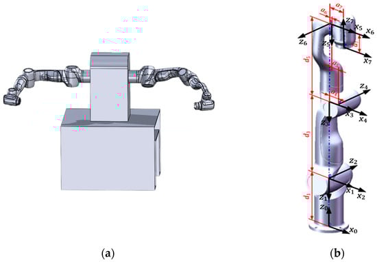
Figure 1.
Dual-arm robot model. (a) shows the three-dimensional model of the two arms; (b) shows the D–H parametric coordinate system for the main arm.

Table 1.
Robot DH parameters.
Since all seven joints of this robotic arm are rotary joints, θ is a variable, and d is a constant. According to the chain rule of D–H coordinate system transformation, the transformation matrix of the seven-degree-of-freedom robotic arm from the coordinate system to the coordinate system is shown in Equation (1):
Finally, the transformation matrix is sequentially solved and multiplied to establish the forward kinematic equations to obtain the position of the end coordinate system of the robotic arm in the base coordinate system. The formula is as follows:
3. Algorithm Improvement
3.1. Two-Stage Sampling-Direction Strategy
The conventional RRT adopts a uniform global random-sampling strategy to rapidly expand new nodes and form feasible paths. However, in cluttered environments, this inherent randomness can render the search blind and inefficient. To address this limitation, we propose a two-stage sampling-direction strategy that guides the tree toward the goal with higher probability and speed.
- Stage I (desired growth). The exploration tree grows greedily toward the goal configuration.
- Stage II (direction optimization). When the tree encounters an obstacle, the planner switches to Stage II and computes a new sampling direction by combining goal bias with random perturbations. If this expansion succeeds, the algorithm returns to Stage I for the next greedy growth cycle. The two-stage loop proceeds iteratively until the goal is reached.
The overall workflow of this two-stage strategy is illustrated in Figure 2.
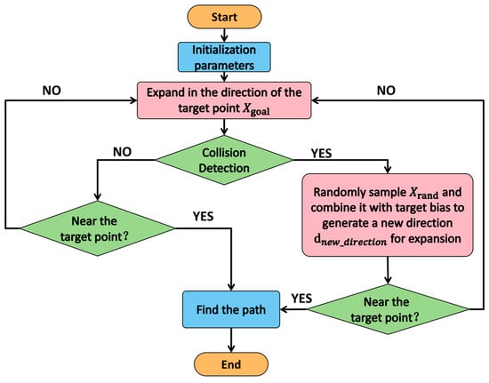
Figure 2.
Flowchart of the two-stage sampling-direction strategy.
In Stage II, when the current expansion collides with an obstacle, the corresponding candidate node is immediately discarded. Subsequently, a random configuration is sampled in the free space. The algorithm then identifies —the existing tree node that is closest to in the Euclidean sense. Based on , the initial sampling direction is generated, as expressed by the following equation:
where ‖·‖ is the Euclidean (2-) norm. The goal-biased direction is defined by the following equation:
The new expansion direction is obtained by summing the unit vectors defined in Equations (3) and (4), as expressed in Equation (5).
By the inner-product bound for unit vectors (, always retains a strictly positive projection onto . Only in the degenerate case , which makes , is the sample discarded and resampled. Consequently, with fixed, the new sampling direction will naturally lie within the half-plane to the right of the perpendicular line L2 drawn through the line L1 connecting and , thereby ensuring that each newly generated node progresses in the positive direction toward the goal. Figure 3 illustrates the Stage II direction-optimization scheme, and the resulting sampling-direction rule is given in Equation (6).
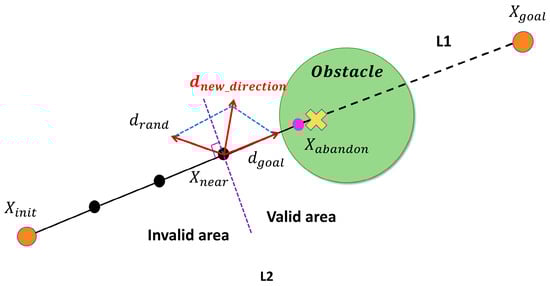
Figure 3.
Optimization of sampling direction.
The proposed strategy preserves the exploratory strength of random sampling while introducing a goal bias that steers each expansion toward the favorable region containing the goal configuration. This guidance enables the search tree to bypass obstacles in cluttered environments and rapidly discover feasible paths. In contrast to a purely goal-attractive (gravity) approach, the method mitigates excessive greediness and exploits stochasticity to explore alternative pathways.
3.2. Dynamic Safety Step-Size Strategy
In conventional RRT variants, a constant step size cannot accommodate varying obstacle distributions in cluttered environments. Consequently, expansions in high-dimensional joint space may produce large configuration jumps, overly long paths, and a higher collision-detection false-negative rate. To address these limitations, we adaptively scale the expansion step size according to the obstacle’s minimum enclosing diameter and the approach angle, thereby improving collision-checking reliability, path safety, and environmental adaptability.
3.2.1. Global Upper Bound for Joint-Space Step Size
First, we require that the workspace displacement induced by a fixed joint-space step be smaller than , the diameter of the smallest obstacle’s bounding sphere. This constraint limits the robot’s posture change at each expansion step, ensuring that the step size is never excessively large; consequently, the planner cannot “over-step” thin protrusions or miss potential contacts, thereby reducing the risk of collision. The mapping between the joint configuration and the workspace pose is obtained through forward kinematics; the relation is given by the following equation:
where is the joint vector and is the end-effector pose. Taking the differential of Equation (7) results in the following expression:
Here, is the geometric Jacobian, denotes the incremental displacement in workspace, and is the corresponding joint-angle increment. Applying the Moore–Penrose pseudoinverse of the Jacobian to Equation (8) yields:
where provides the minimum-norm joint-space increment for a given workspace displacement. Because the workspace displacement must satisfy, we apply this constraint to Equation (9). Taking the Euclidean (2-) norm of both sides of Equation (9) yields the following upper bound on the joint-space step size:
Here, , where is the smallest non-zero singular value of . To provide an additional margin of safety, we introduce an empirical coefficient and scale the constrained step size accordingly; the resulting expression is given by the following equation:
3.2.2. Segmented Dynamic Step-Size Adjustment
Building on the two-stage expansion-direction strategy, we rescale the expansion step size during Stage II according to the angle between the new expansion direction and the goal-biased direction . This adaptive mechanism promotes accelerated growth when the tree points toward the goal and more conservative exploration when it diverges, thereby improving overall planning efficiency. Specifically, Stage I employs the constrained step size to extend directly toward . Once a collision is detected and the planner enters Stage II, the angle θ between and is computed, and the step size is dynamically adjusted according to this angle. The calculation of θ is given by the following expression:
Subsequently, the extension step size is dynamically adjusted in segmented ranges based on the value of θ. In this work, the scaling factors corresponding to each segment are denoted as , and their values are determined through extensive experimental experience to achieve a balance between extension efficiency and path quality. In this study, we evaluate configurations with two, three, and four segments. Table 2 summarizes the mean results obtained from 100 trials conducted in a 3-D obstacle environment. Among them, the smoothness index is defined as the average cosine of the turning angles at all internal vertices of the path. A higher index value corresponds to a smoother trajectory, whereas a lower value reflects the presence of sharper turns and reduced smoothness.
Table 2.
Statistical indicators for the three segments.
The parameters in each segmentation scheme represent the scaling factors applied to the expansion step length over different deviation angle intervals. In the two-segment scheme, and correspond to the ranges of 0–45° and 45–90°, respectively. In the three-segment scheme, and are assigned to the ranges of 0–30°, 30–60°, and 60–90°, respectively. In the four-segment scheme, and correspond to the ranges of 0–25°, 25–50°, 50–75°, and 75–90°, respectively. These values were empirically determined to balance expansion efficiency and path quality across complex 3-D environments. Bold numbers denote the best (optimal) performance among the three segmentation schemes.
As shown in Table 2, the three-segment configuration yields only marginally shorter paths than the two- and four-segment cases; nevertheless, it reduces the number of sampled nodes by 26% and 22% and improves the path-smoothness metric by 9.2% and 10.4%, respectively. These results indicate that the three-segment scheme offers the best overall performance. Consequently, we adopt the three-segment dynamic step size, denoted, as the default setting, where is defined as:
As θ increases, the expansion direction diverges further from the goal; consequently, the step size is proportionally reduced to prevent large configuration jumps and fruitless expansions. Relative to a constant step size, this dynamic adaptation markedly improves path smoothness and safety margin without compromising planning speed, producing trajectories that are both continuous and collision-safe.
3.3. Expansion-Node Optimization Strategy
The standard RRT expansion often produces numerous redundant or infeasible nodes, which increases planning time and may cause the search to be trapped in local minima within cluttered environments. To address this issue, we introduce an expansion-node optimization strategy in Stage II. The strategy generates a set of candidate nodes , evaluates them, and inserts the optimal node into the exploration tree T, thereby preserving probabilistic completeness while improving overall path quality. The specific process is as follows:
- Sampling. During Stage II, randomly sample joint-space configurations . The value of is chosen adaptively according to the density of environmental obstacles.
- Candidate generation. For each sample, combine the goal-biased direction with the random direction to obtain a new expansion direction . Using the dynamic step size , generate a corresponding set of candidate nodes, as defined by Equation (14):
- Selection. Discard any candidate nodes that collide with obstacles. For the remaining collision-free candidates, compute their Euclidean distances to the goal and insert into the tree the node with the smallest distance, denoted , according to Equation (15).
For completeness, the expansion rule is provided in Equation (16).
As illustrated in Figure 4, and assuming, the candidate node is discarded because it is in collision. Since the Euclidean distance from to the goal is smaller than that from , is selected as the new expansion node.
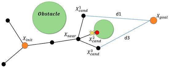
Figure 4.
Illustration of the expansion-node optimization strategy.
A backtracking recovery mechanism is incorporated to prevent the search from stagnating. As depicted in Figure 5, if the exploration tree enters a local trap and the collision-free candidate set C becomes empty, the attempt is recorded as an expansion failure and the planner immediately re-expands. When the number of consecutive failures reaches the predefined limit , the node is deemed invalid, and the algorithm retreats to its parent node for resampling until a successful expansion is achieved. This strategy markedly reduces redundant nodes and fruitless explorations, thereby enhancing both the efficiency and the robustness of the overall path-planning process.
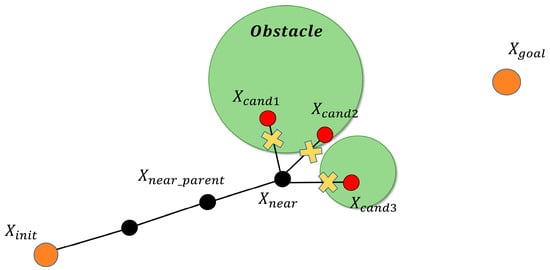
Figure 5.
Illustration of the invalid expansion-node case.
3.4. Dual-Arm Collision-Detection Model
Dual-arm robots exhibit high structural redundancy with many links and degrees of freedom, so conventional collision-detection schemes—based on detailed geometry—are computationally expensive and inefficient. To mitigate both self-collision and robot-environment collision during path planning, we adopt a cylindrical–spherical bounding-volume framework. Each link is approximated by a cylinder whose axis coincides with the link center line and whose radius equals its maximum cross-sectional envelope, whereas every environmental obstacle, irrespective of shape, is enclosed by its minimum bounding sphere.
Under this concept, robot-to-obstacle checking reduces to computing the minimum distance between a line segment (link axis) and a sphere centroid, while self-collision checking reduces to the minimum distance between two line segments. The resulting formulation greatly simplifies spatial occupancy queries, accelerates collision detection, and consequently enhances both the efficiency of obstacle-avoidance planning and the operational safety of dual-arm cooperation.
3.4.1. Link–Obstacle Collision Detection
Figure 6 presents the simplified geometric model used for collision checking. Let O denote the center of the spherical obstacle, and let AB represent the axis of the cylindrical link; point C is the foot of the perpendicular dropped from O onto AB. The link’s cylinder has a maximum radial envelope of , whereas the obstacle’s bounding sphere has radius . The minimum distance between the obstacle center and the link axis is
A collision is declared when
and a safety margin is added to prevent the link from approaching the obstacle too closely, as defined by Equation (19):
this criterion enables efficient detection of robot–obstacle contacts while maintaining a protective clearance for the dual-arm system.
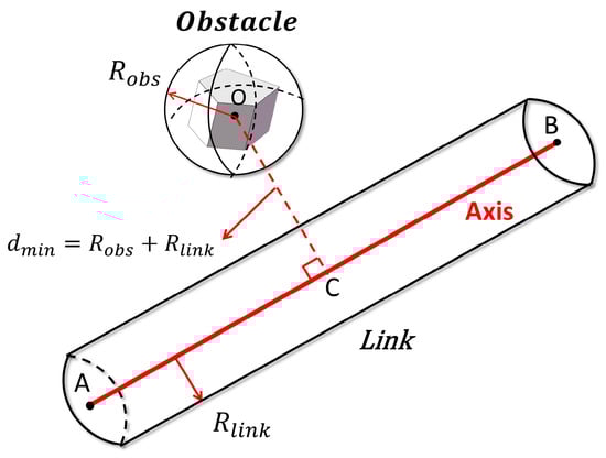
Figure 6.
Illustration of the link–obstacle collision model.
The simplified model yields four distinct relative configurations between the cylindrical link and the spherical obstacle, illustrated in Figure 7. In each sub-figure, the blue dashed line represents , where C is the orthogonal projection of the obstacle center O onto the link axis AB. Let ; based on the value of , it can be determined whether C is between A and B. As in Table 3, the four cases are summarized. The four cases in the Figure 7 also correspond to (a–d) in the table.
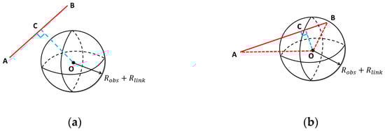
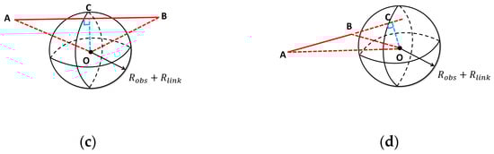
Figure 7.
Link–obstacle relative configurations. (a) No collision (clearance exceeds the sum of radii); (b) single-point collision (one intersection of link axis and obstacle surface); (c) two-point collision (link axis passes through the sphere); (d) no collision (projections outside the link segment).
Table 3.
Detailed descriptions of link–obstacle collision cases.
Finally, the shortest clearance distance between the link and the obstacle is computed as follows:
where denotes the normalized projection of the obstacle center O onto the link axis AB. The condition indicates that the projection point C lies on the interior of segment AB; otherwise (), C falls outside the segment.
3.4.2. Link–Link Collision Detection
Figure 8 depicts the simplified model used for link–link collision checking. Let A and B be the endpoints of each cylindrical link’s axis segment, and let M denote the segment’s midpoint. Self-collision evaluation reduces to comparing the distance between the central axes of two cylinders with the sum of their radii. For any pair of non-adjacent links on the same arm—or links belonging to different arms—a collision is declared when the center-line distance is smaller than the sum of the respective radii. A safety margin is added to prevent the links from approaching too closely. The collision criterion is expressed by the following equation:
where is the minimum axial distance between the two cylindrical links, and are their respective radii, and is the prescribed safety margin.
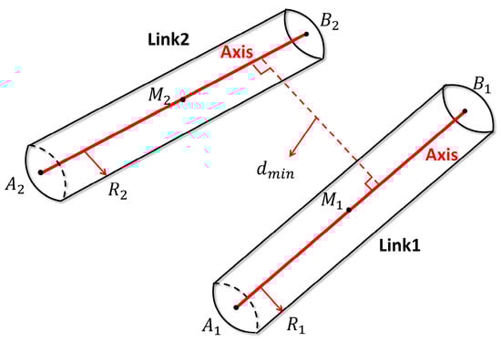
Figure 8.
Illustration of the link–link collision model.
The minimum distance between two line segments can be cast as a constrained optimization problem. As shown in Figure 8, for two cylindrical links, let the first link be the line segment and the second link be . Any point on the first segment can be parametrized as:
while any point on the second segment is:
The squared distance between the two parametric points is:
Let ,, . Minimizing with respect to and by setting the partial derivatives and yields the optimal parameters; the formulas are as follows:
Figure 9 illustrates the three possible configurations for the minimum distance between two line segments. The specific situation is as follows:
- 1.
- Case (a): If , the foot-points of the mutual perpendicular lie inside both segments. The solution of the optimization problem is valid, yielding .
- 2.
- Case (b): If , and, using the point-to-segment distance formula for each of the four endpoints yields the following equation:where denotes the Euclidean distance from point P to segment .
- 3.
- Case (c): If the link-to-link distance is the minimum of the four endpoint–endpoint distances, and the formula is as follows:

Figure 9.
Illustrations of the three minimum-distance cases between line segments. (a) Interior–interior (: both projections lie within their segments; (b) mixed exterior : one projection falls outside its segment; (c) exterior–exterior : both projections lie outside their segments.
Figure 9.
Illustrations of the three minimum-distance cases between line segments. (a) Interior–interior (: both projections lie within their segments; (b) mixed exterior : one projection falls outside its segment; (c) exterior–exterior : both projections lie outside their segments.

3.5. Path Optimization
Although the enhanced ODSN-RRT algorithm can generate a feasible trajectory rapidly, the raw path often contains numerous redundant vertices, which introduce unnecessary bends. To address this, we apply a progressive node-pruning strategy combined with segmented collision checking. The procedure is outlined below.
- Forward pruning.
Let the initial path be . Starting from the first reference node , we examine downstream nodes in reverse order—from those farthest from back toward . If the straight-line segment is collision-free, the intermediate vertices are removed, producing an updated path
- 2.
- Iterative refinement.
The algorithm then selects the next vertex after in as the new reference node and repeats the above test, yielding , …, until is reached; the final result is . A schematic diagram of the path optimization process is shown in Figure 10.
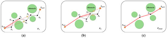
Figure 10.
Illustration of the path-optimization process. The black dashed polyline denotes the initial trajectory generated by ODSN-RRT, while the red solid polyline represents the optimized trajectories. (a) Initial path ; (b) intermediate path after one pruning iteration; (c) final smoothed path .
Node-based collision checking alone can miss obstacles when two far-apart vertices are rewired, because the straight-line segment between them may intersect unseen obstacles. To prevent such omissions, we introduce a segmented interpolation check at every long-segment rewiring step.
Consider an attempted shortcut connecting to . Let be the number of intermediate vertices slated for removal. We divide the segment into equal parts and insert the interpolation points at the subdivision boundaries. If all of these interpolated points are collision-free, the shortcut is accepted and the original intermediate verticesare deleted; otherwise, the connection is rejected. This segmented check ensures that every newly formed path section remains feasible throughout its entire length.
3.6. Algorithm Implementation
The proposed planner augments the classical RRT framework with a two-stage expansion scheme that alternates between (i) greedy goal-directed growth and (ii) direction-optimized sampling. This organization accelerates exploration in free space while preserving probabilistic completeness in cluttered, high-dimensional joint spaces. The specific process is as follows:
- Initialization.
The search tree is initialized as, where and denote the start and goal configurations, respectively. The node nearest to the expansion front is stored as .
- 2.
- Stage I—Goal-directed expansion.
From the tree is extended toward using the constrained step length . If the straight-line segment is collision-free, the new node is appended to and becomes the next ; Stage I is repeated. Otherwise, a collision is detected and the algorithm switches to Stage II.
- 3.
- Stage II—Direction-optimized sampling.
- (1)
- Generate random samples in joint space.
- (2)
- For each sample, construct a goal-biased direction by combining the random vector with ; compute the adaptive step length from the angle θ between these vectors.
- (3)
- Generate the candidate node set and discard any colliding nodes.
- (4)
- Select .
- (5)
- If , record a failure; once consecutive failures exceed backtrack to the parent of and resample.
- (6)
- Add and return to Stage I.
- 4.
- Termination.
Repeat the Stage I and Stage II cycle until is attached to ; extract and post-process the final path.
Algorithm 1 below describes the ODSN-RRT algorithm in detail.
| Algorithm 1. ODSN-RRT |
| Output: T |
| do #Stage I: goal-directed growth |
| do |
| ) then |
| ) < threshold then |
| 8. return T |
| 9. end if |
| 10. else |
| 11. break #collision → switch to Stage II |
| 12. end if |
| 13. end while |
| do #Stage II: direction-optimized growth |
| = 1 to k do |
| ) |
| then |
| 25. end if |
| 26. end for |
| then |
| ) < threshold then |
| into T, return T |
| 32. end if |
| 33. else #Failure backtracking |
| + 1 |
| then |
| then |
| 38. else |
| 39. return “failure” |
| 40. end if |
| 41. end if |
| 42. end if |
| 43. break |
| 44. end while |
| 45. end for |
4. Simulation and Experimental Validation
This section compares the proposed ODSN-RRT algorithm with four widely used planners—classical RRT, RRT*, Goal-Biased RRT, and Informed-RRT*—in 2-D and 3-D complex environments, and validates the superiority of ODSN-RRT. In addition, the algorithm is validated on the laboratory Diana dual-arm robot through MATLAB simulations and corresponding experiments. All simulations were executed under Python 3.9 and MATLAB R2024a on a workstation equipped with an Intel Core i7-12700H processor.
4.1. 2-D Environment Simulation
A 100 × 100 two-dimensional workspace is populated with several green circular obstacles that represent impassable regions; the image border defines the workspace boundary. For the Goal-Biased RRT implementation, the goal-sampling probability is set to 0.05, the initial step length to 10, the start configuration to (5, 5), the goal configuration to (95, 95), and the maximum iteration count to 500. Path-planning trials are conducted with five planners—RRT, RRT*, Goal-Biased RRT, Informed-RRT*, and the proposed ODSN-RRT—and the resulting trajectories are illustrated in Figure 11. Each algorithm is executed in 100 independent runs. The mean path length, number of sampled nodes, and a path-smoothness metric are recorded. The aggregate statistics are summarized in Table 4.
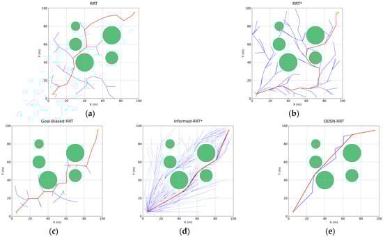
Figure 11.
Planning results of five algorithms in a 2-D environment: (a) RRT; (b) RRT*; (c) Goal-Biased RRT; (d) Informed-RRT*; (e) ODSN-RRT. Among them, the red line represents the planned path, the blue line represents the exploration tree T, and the green circle represents obstacles.
Table 4.
Performance of five algorithms in a 2-D environment.
As shown in Figure 11 and Table 4, the proposed ODSN-RRT outperforms all baselines in the 2-D benchmark. Compared with the classical RRT, it lowers the mean node count by 80.3%, shortens the average path length by approximately 15.6%, and raises the smoothness metric by 32.4%. Compared with the RRT* and the Goal-Biased RRT, ODSN-RRT still achieves the best overall performance, lowering node counts by 80.2% and 72.9%, shortening paths by 7.3% and 11.9%, and increasing smoothness by 11.9% and 23.7%, respectively. Finally, compared with the more sophisticated Informed-RRT*, although ODSN-RRT improves path length and smoothness by only 2.1% and 5.6%, it reduces the node count by 95.6%, greatly enhancing node utilization and computational efficiency. These results confirm that ODSN-RRT offers the highest search efficiency and trajectory quality among all evaluated planners.
4.2. 3-D Environment Simulation
The proposed algorithm is further evaluated in a 100 × 100 × 100 three-dimensional workspace under two obstacle scenarios, denoted A and B. Scenario A contains five green spheres of varying radii, whereas Scenario B contains ten; these spheres define impassable regions. The start and goal configurations are fixed at (5, 5, 5) and (95, 95, 95), respectively, and the iteration limit is increased to 1000; all remaining parameters match those used in the 2-D experiments. The five planners—RRT, RRT*, Goal-Biased RRT, Informed-RRT*, and ODSN-RRT—are applied to both scenarios, and their resulting trajectories are illustrated in Figure 12 and Figure 13.
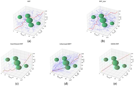
Figure 12.
Planning results of five algorithms in 3-D scenarios. Panels (a–e) show path plans for Scenario A (five spherical obstacles): (a) RRT; (b) RRT*; (c) Goal-Biased RRT; (d) Informed-RRT*; (e) ODSN-RRT. Among them, the red line represents the planned path, the blue line represents the exploration tree T, and the green spheres represent obstacles.
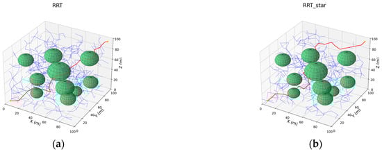
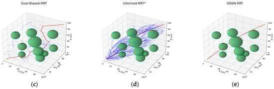
Figure 13.
Planning results of five algorithms in 3-D scenarios. Panels (a–e) show path plans for Scenario B (ten spherical obstacles): (a) RRT; (b) RRT*; (c) Goal-Biased RRT; (d) Informed-RRT*; (e) ODSN-RRT. Among them, the red line represents the planned path, the blue line represents the exploration tree T, and the green spheres represent obstacles.
As illustrated in Figure 12 and Figure 13, the classical RRT generates a very dense search tree in the 3-D test scenes, producing many redundant nodes and, consequently, long and tortuous trajectories. RRT* rewires the tree and shortens the path, but its exploration remains scattered. Introducing only a goal bias, the Goal-Biased RRT partially improves the expansion direction but still suffers from local stagnation and yields paths that remain insufficiently smooth. Informed-RRT* focuses its sampling inside the heuristic ellipsoid and therefore generates a much narrower tree; however, it requires many more nodes to converge and occasionally skirts obstacles very closely. By contrast, the proposed ODSN-RRT is not only shorter and smoother but also preserves a larger safety margin around obstacles. To quantify these differences, each of the five planners—RRT, RRT*, Goal-Biased RRT, Informed-RRT*, and ODSN-RRT—was executed 100 times in both obstacle scenarios A and B. Mean values of path length, node count, smoothness, planning time, and success rate were computed. The aggregated statistics are reported in Table 5 and Table 6.
Table 5.
Performance of five algorithms in Scenario A.
Table 6.
Performance of five algorithms in Scenario B.
As indicated by Table 5 and Table 6, the proposed ODSN-RRT achieves the best overall performance in both complex 3-D scenarios.
- Scenario A. Relative to the classical RRT, the average path length is shortened by 21.0%, the mean number of sampled nodes is cut by 96.5%, the path-smoothness metric is raised by 95.6%, and planning time falls 95.7%. Against RRT*, the path is 31.9% shorter, nodes fall by 96.2%, smoothness nearly doubles, and time is cut 98.9%. Relative to Goal-Biased RRT, the path is 19.6% shorter, nodes are reduced by 65.3%, smoothness improves by 26.8%, and time is slightly higher. Finally, compared with the Informed-RRT*, ODSN-RRT still trims 2.0% off the path while cutting node count from 911 to 17 (−98.1%), raising the smoothness metric from 0.85 to 0.89 and cutting planning time by 99.9%.
- The denser Scenario B. ODSN-RRT achieves the lowest mean path length and maintains a node count of only 22. This represents a 32.9% reduction in path length and a 94.6% reduction in nodes compared with RRT, together with more than double the smoothness. Versus RRT*, the path is 32.7% shorter, nodes fall by 94.5%, and smoothness again more than doubles. Compared with Goal-Biased RRT, the path shortens by 21.7%, nodes drop by 76.3%, smoothness rises by 29.9%, and planning time is 41.8% faster. Relative to Informed-RRT*, the path is 1.2% shorter, node count is reduced by 97.5%, comparable smoothness is maintained, and planning is sped up by 99.8% while preserving a 100% success rate.
These results confirm that ODSN-RRT consistently yields shorter, smoother trajectories with far fewer nodes, orders-of-magnitude lower computation time, and perfect planning success, thereby maintaining its efficiency and path-quality advantages even in highly complex three-dimensional environments.
4.3. Ablation Experiments
To more clearly demonstrate the functionality of the various components of the algorithm proposed in this paper, we carried out an ablation study in the more challenging three-dimensional Scenario B. Starting from the baseline RRT, the modules for direction guidance (OD-RRT), dynamic step size (ODS-RRT), and node optimization (ODSN-RRT) were successively enabled, thereby revealing the cumulative efficiency gains obtained by the full algorithm. Each configuration was executed 100 times, and the resulting average values of all evaluation metrics are reported in Table 7.
Table 7.
Performance of RRT, OD-RRT, ODS-RRT, and ODSN-RRT in Scenario B.
As indicated by Table 7, introducing the direction-guidance module alone reduces the average path length from 246.36 m to 177.50 m (−28%), shrinks the tree from 356 to 20 nodes (−94%), improves smoothness from 0.55 to 0.69, and cuts planning time from 0.047 s to 0.003 s. Adding the dynamic step further shortens the path to 168.40 m (−5% relative to OD-RRT), and raises smoothness to 0.76. Finally, enabling node optimization yields the full ODSN-RRT, which attains the best overall metrics. Compared with the original RRT, this represents a 33% shorter path, 93% fewer nodes, a 58% increase in smoothness, and a 94% reduction in computation time. These results demonstrate that all three modules have a positive guiding effect: the direction-guidance module provides the greatest efficiency gain, the dynamic step-size optimization markedly improves path quality while maintaining high efficiency, and the node-selection optimization further increases smoothness and yields an even better path. Together, they confirm both the necessity and the complementarity of every component within the proposed ODSN-RRT framework.
4.4. Dual-Arm Robot Simulation
The proposed algorithm has been validated in both two- and three-dimensional benchmark scenes. To assess its suitability for high-degree-of-freedom manipulators, we further test it on a dual-arm robot whose left and right arms each possess seven joints. A master–slave planning strategy is adopted: the left arm acts as the master, the right arm as the slave. The procedure is as follows:
- Master-arm planning: A collision-free trajectory for the master arm is generated while considering all static spherical obstacles.
- Slave-arm planning: At every time step, the instantaneous configuration of the master arm is treated as a dynamic obstacle; the slave arm is then planned so that it avoids both the environment and the moving master arm.
By decomposing the original fourteen-dimensional joint-state space into two seven-dimensional sub-problems, this approach sidesteps the exponential complexity of simultaneous planning, markedly reducing computational effort while guaranteeing mutual collision avoidance. The overall master–slave workflow is illustrated in Figure 14.
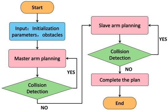
Figure 14.
Master–slave planning flowchart for dual-arm manipulators.
To assess the proposed algorithm in a dual-arm obstacle-avoidance context, we build a simulation model of the laboratory’s dual-arm robot and embed it in a workspace populated with spherical obstacles. The initial joint configurations and obstacle parameters used in this scenario are summarized in Table 8.
Table 8.
Initial configurations and obstacle layout for the dual-arm simulation.
Obstacles are positioned along the straight-line route to the goal configuration, creating a challenging workspace for motion planning. Employing MATLAB’s Robotics Toolbox, the ODSN-RRT algorithm is run to generate a collision-free trajectory for the dual-arm robot. The safety margin is set to , the consecutive-failure limit to , and the global iteration cap to The complete obstacle-avoidance sequence is presented in Figure 15, and the end-effector paths are detailed in Figure 16.
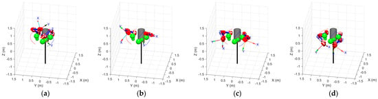
Figure 15.
Dual-arm obstacle-avoidance sequence. The blue curve traces the master (left) arm trajectory, the red curve traces the slave (right) arm trajectory, and the green spheres denote obstacles. (a) Initial arm configurations; (b,c) intermediate obstacle-avoidance maneuvers; (d) final target configurations.
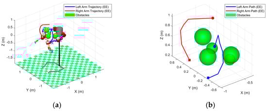
Figure 16.
Illustration of dual-arm end-effector trajectories. (a) Global view of both arms’ planned paths in the workspace; (b) local zoom on the end-effector trajectories near the goal region.
Traditional motion planners often verify collisions only along the end-effector trajectory and overlook potential contacts involving the robot’s links. Consequently, once a collision-free path has been found for the end effector, each intermediate joint must still be screened against the workspace obstacles. For the laboratory robot, joints 1 and 2 are fixed rotary axes mounted flush with the torso; their envelopes do not enter the obstacle field and can therefore be excluded from the joint-level check. The remaining joints are evaluated with the cylindrical–spherical model described earlier. As illustrated in Figure 17, all active joints of both arms remain outside the obstacle envelopes throughout the motion, maintaining a satisfactory safety margin.
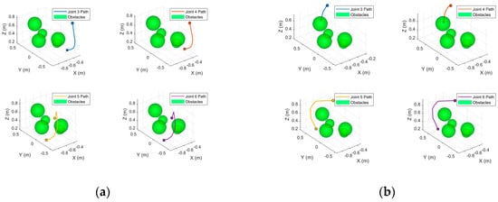
Figure 17.
Joint trajectory profiles for master and slave arms: (a) full trajectory of each joint for the master arm; (b) full trajectory of each joint for the slave arm.
Figure 18 and Figure 19 compare the fourteen joint trajectories before and after path optimization. The master arm executes a more complex avoidance sequence than the slave arm, yet its motion remains continuous and well behaved. Relative to the pre-optimized curves, the post-optimized joint profiles for both arms display markedly reduced fluctuations, confirming that the smoothing stage yields steadier and more uniform motion.
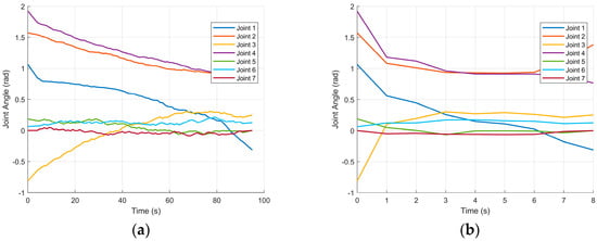
Figure 18.
Master-arm joint angle profiles before and after optimization. (a) Joint angles of the master arm before smoothing; (b) joint angles of the master arm after smoothing.
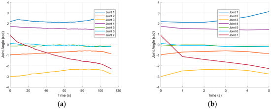
Figure 19.
Slave-arm joint angle profiles before and after optimization. (a) Joint angles of the slave arm before smoothing; (b) joint angles of the slave arm after smoothing.
The simulation studies show that the proposed ODSN-RRT consistently produces collision-free trajectories for both the master and the slave arms, guiding them smoothly and stably from their initial to their target configurations. The method markedly reduces search effort, enhances path quality, and retains its advantages even in the complex, high-dimensional workspace of a dual-arm system. These findings confirm the feasibility and effectiveness of the improved RRT scheme and provide a sound theoretical and algorithmic foundation for forthcoming hardware validation.
4.5. Real-Robot Experimental Validation
The hardware trials were carried out on a Diana dual-arm robot, comprising two mirrored seven-DOF manipulators, as illustrated in Figure 20. A supervisory PC commands the robot, while the ODSN-RRT planner is implemented in MATLAB. Collision-free trajectories are generated offline, uploaded to the host computer, and subsequently transmitted to the robot’s control system for execution.
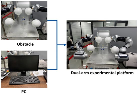
Figure 20.
Dual-arm robot experimental platform.
Four spherical obstacles were arranged within the dual-arm workspace. The proposed ODSN-RRT planner was then applied to generate an obstacle-avoidance trajectory. The simulated path is depicted in Figure 21, while Figure 22 presents the corresponding execution sequence on the physical robot, and Figure 23 shows the resulting joint-angle profiles. Across all trials, the computed trajectory remained smooth and collision-free, and the arms successfully avoided both environmental obstacles and mutual interference. These outcomes confirm the effectiveness and superiority of the proposed algorithm in a real-robot setting.
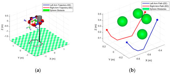
Figure 21.
Simulation path of the dual-arm robot. (a) Global view of the planned trajectories for both arms; (b) local detail of the end-effector path.
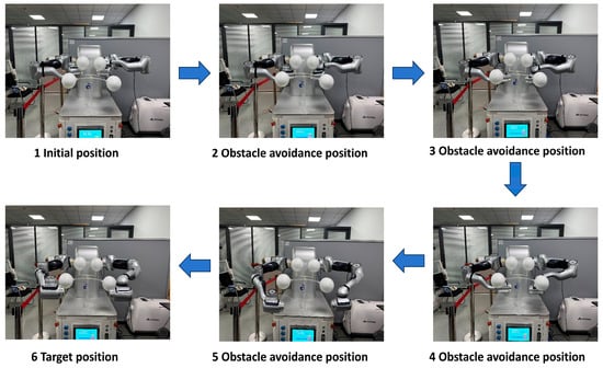
Figure 22.
Actual path-planning sequence for dual-arm manipulators.
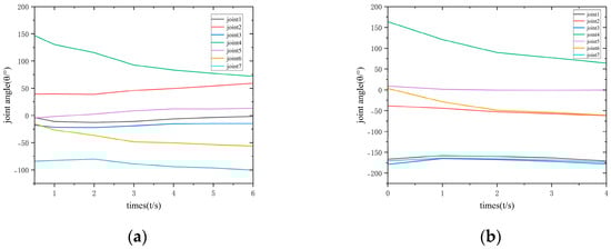
Figure 23.
Joint-angle variations for left and right arms. (a) Joint-angle variation of the left arm; (b) joint-angle variation of the right arm.
5. Conclusions and Future Work
This study presents ODSN-RRT, which co-optimizes three key aspects of RRT sampling—direction, dynamic step size, and candidate-node selection—to achieve efficient obstacle-avoidance planning for dual-arm manipulators in cluttered workspaces. Direction and node optimization accelerate tree growth in free space and improve path quality, while adaptive step-sizing, guided by safety constraints and angular scaling, maintains robustness in densely obstructed or narrow passages. A cylindrical–spherical bounding-volume model simplifies collision checking by reducing link–obstacle and self-collision queries to efficient line–sphere and line–line distance tests. Post-processing removes redundant vertices and applies a master–slave strategy that decomposes the 14-DOF problem into two 7-DOF subplans, ensuring smooth, coordinated motion. Extensive simulations and hardware trials on a 7-DOF dual-arm robot confirm that ODSN-RRT delivers higher search efficiency, shorter paths, superior smoothness, faster planning times, and higher success rates compared with state-of-the-art planners. Accordingly, the method offers a practical solution for dual-arm manipulation in automated chemical experiments and similarly complex tasks.
Future work will extend the proposed ODSN-RRT framework to more dynamic and uncertain environments. In particular, we intend to incorporate moving obstacles into our planning scenarios and account for real-world uncertainties such as sensor noise and localization errors. This will involve integrating real-time perception and on-the-fly re-planning mechanisms so that the robot can adjust its trajectory if conditions change during execution. In addition, we will also explore multi-robot coordination and learning-based strategies (e.g., deep reinforcement learning) to further improve the method’s real-time performance and robustness in unknown, time-varying environments.
Author Contributions
Conceptualization, J.W.; methodology, J.W.; software, J.W.; validation, J.W., J.C. and J.Z.; formal analysis, J.W.; investigation, J.W.; resources, J.W.; data curation, J.W.; writing—original draft preparation, J.W.; writing—review and editing, J.W., G.X. and H.X.; visualization, J.W.; supervision, B.D.; project administration, J.W.; funding acquisition, G.X. All authors have read and agreed to the published version of the manuscript.
Funding
This work was supported by the Capacity Building Plan for local colleges and universities of Shanghai Scientific Committee (Grant No. 23010501600), National Natural Science Foundation of China (Grant Nos. 61263045, 61763030), and National Key Research and Development Program of China (Grant No. 2018YFB1305300).
Data Availability Statement
The raw data contributions presented in the study are included in the article; further inquiries can be directed to the corresponding authors.
Conflicts of Interest
The authors declare no conflicts of interest.
Correction Statement
This article has been republished with a minor correction to the correspondence affiliation. This change does not affect the scientific content of the article.
References
- Yang, S.; Zhang, Y.; Wen, H.; Jin, D. Coordinated control of dual-arm robot on space structure for capturing space targets. Adv. Space Res. 2023, 71, 2437–2448. [Google Scholar] [CrossRef]
- Peta, K.; Wiśniewski, M.; Kotarski, M.; Ciszak, O. Comparison of Single-Arm and Dual-Arm Collaborative Robots in Precision Assembly. Appl. Sci. 2025, 15, 2976. [Google Scholar] [CrossRef]
- Krüger, J.; Schreck, G.; Surdilovic, D. Dual arm robot for flexible and cooperative assembly. CIRP Ann. Manuf. Technol. 2011, 60, 5–8. [Google Scholar] [CrossRef]
- Abbas, M.; Narayan, J.; Dwivedy, S.K. A systematic review on cooperative dual-arm manipulators: Modeling, planning, control, and vision strategies. Int. J. Intell. Robot. Appl. 2023, 7, 683–707. [Google Scholar] [CrossRef]
- Jiang, Y.; Fakhruldeen, H.; Pizzuto, G.; Longley, L.; He, A.; Dai, T.; Clowes, R.; Rankin, N.; Cooper, A.I. Autonomous biomimetic solid dispensing using a dual-arm robotic manipulator. Digit. Discov. 2023, 2, 1733–1744. [Google Scholar] [CrossRef]
- Fleischer, H.; Baumann, D.; Joshi, S.; Chu, X.; Roddelkopf, T.; Klos, M.; Thurow, K. Analytical measurements and efficient process generation using a dual–arm robot equipped with electronic pipettes. Energies 2018, 11, 2567. [Google Scholar] [CrossRef]
- Fleischer, H.; Baumann, D.; Chu, X.; Roddelkopf, T.; Klos, M.; Thurow, K. Integration of Electronic Pipettes into a Dual-arm Robotic System for Automated Analytical Measurement Processes Behaviors. In Proceedings of the 2018 IEEE 14th International Conference on Automation Science and Engineering (CASE), Munich, Germany, 20–24 August 2018; pp. 22–27. [Google Scholar]
- Liu, J.; Xu, C.; Jia, X.; Wu, Y.; Li, T. Cooperative Collision Avoidance Control with Relative Velocity Information for Redundant Dual-arm Robotic Manipulators. J. Bionic Eng. 2025, 22, 1111–1125. [Google Scholar] [CrossRef]
- Lei, M.; Wang, T.; Yao, C.; Liu, H.; Wang, Z.; Deng, Y. Real-Time Kinematics-Based Self-Collision Avoidance Algorithm for Dual-Arm Robots. Appl. Sci. 2020, 10, 5893. [Google Scholar] [CrossRef]
- Lin, Y.; Zhang, Z.; Tan, Y.; Fu, H.; Min, H. Efficient TD3 based path planning of mobile robot in dynamic environments using prioritized experience replay and LSTM. Sci. Rep. 2025, 15, 18331. [Google Scholar] [CrossRef]
- Liu, L.; Wang, X.; Yang, X.; Liu, H.; Li, J.; Wang, P. Path planning techniques for mobile robots: Review and prospect. Expert Syst. Appl. 2023, 227, 120254. [Google Scholar] [CrossRef]
- Orthey, A.; Chamzas, C.; Kavraki, L.E. Sampling-based motion planning: A comparative review. Annu. Rev. Control Robot. Auton. Syst. 2024, 7, 285–310. [Google Scholar] [CrossRef]
- Zhou, C.; Huang, B.; Fränti, P. A review of motion planning algorithms for intelligent robots. J. Intell. Manuf. 2022, 33, 387–424. [Google Scholar] [CrossRef]
- Szczepanski, R. Safe Artificial Potential Field—Novel Local Path Planning Algorithm Maintaining Safe Distance From Obstacles. IEEE Robot. Autom. Lett. 2023, 8, 4823–4830. [Google Scholar] [CrossRef]
- Liu, Z.; Yang, H.; Wang, Q.; Shi, Y.; Zhao, J. An improved A* algorithm for generating four-track trajectory planning to adapt to longitudinal rugged terrain. Sci. Rep. 2025, 15, 6727. [Google Scholar] [CrossRef]
- Yuan, Q.; Sun, R.; Du, X. Path Planning of Mobile Robots Based on an Improved Particle Swarm Optimization Algorithm. Processes 2023, 11, 26. [Google Scholar] [CrossRef]
- Chen, G.; Luo, N.; Liu, D.; Zhao, Z.; Liang, C. Path planning for manipulators based on an improved probabilistic roadmap method. Robot. Comput.-Integr. Manuf. 2021, 72, 102196. [Google Scholar] [CrossRef]
- Xu, T. Recent advances in Rapidly-exploring random tree: A review. Heliyon 2024, 10, e32451. [Google Scholar] [CrossRef]
- Kuffner, J.J.; LaValle, S.M. RRT-connect: An efficient approach to single-query path planning. In Proceedings 2000 ICRA. Millennium Conference, Proceedings of the IEEE International Conference on Robotics and Automation. Symposia Proceedings (Cat. No.00CH37065), San Francisco, CA, USA, 24–28 April 2000; IEEE: New York, NY, USA, 2000; pp. 995–1001. [Google Scholar]
- Zhang, L.; Cai, K.; Sun, Z.; Bing, Z.; Wang, C.; Figueredo, L.; Haddadin, S.; Knoll, A. Motion planning for robotics: A review for sampling-based planners. Biomimet. Intell. Robot. 2025, 5, 100207. [Google Scholar] [CrossRef]
- Kang, M.; Chen, Q.; Fan, Z.; Yu, C.; Wang, Y.; Yu, X. A RRT based path planning scheme for multi-DOF robots in unstructured environments. Comput. Electron. Agric. 2024, 218, 108707. [Google Scholar] [CrossRef]
- Jiang, L.; Liu, S.; Cui, Y.; Jiang, H. Path planning for robotic manipulator in complex multi-obstacle environment based on improved_RRT. IEEE/ASME Trans. Mechatron. 2022, 27, 4774–4785. [Google Scholar] [CrossRef]
- Armstrong, D.; Jonasson, A. AM-RRT*: Informed sampling-based planning with assisting metric. In Proceedings of the 2021 IEEE International Conference on Robotics and Automation (ICRA), Xi’an, China, 30 May–5 June 2021; pp. 10093–10099. [Google Scholar]
- Shi, W.; Wang, K.; Zhao, C.; Tian, M. Obstacle avoidance path planning for the dual-arm robot based on an improved RRT algorithm. Appl. Sci. 2022, 12, 4087. [Google Scholar] [CrossRef]
- Dong, Z.; Zhong, B.; He, J.; Gao, Z. Dual-Arm Obstacle Avoidance Motion Planning Based on Improved RRT Algorithm. Machines 2024, 12, 472. [Google Scholar] [CrossRef]
- Wang, H.; Zhou, X.; Li, J.; Yang, Z.; Cao, L. Improved RRT* Algorithm for Disinfecting Robot Path Planning. Sensors 2024, 24, 1520. [Google Scholar] [CrossRef] [PubMed]
- Wang, J.; Li, T.; Li, B.; Meng, M.Q.H. GMR-RRT*: Sampling-Based Path Planning Using Gaussian Mixture Regression. IEEE Trans. Intell. Veh. 2022, 7, 690–700. [Google Scholar] [CrossRef]
- Fang, Y.; Lu, L.; Zhang, B.; Liu, X.; Zhang, H.; Fan, D.; Yang, H. Motion control of obstacle avoidance for the robot arm via improved path planning algorithm. J. Braz. Soc. Mech. Sci. Eng. 2024, 46, 727. [Google Scholar] [CrossRef]
- Karaman, S.; Frazzoli, E. Sampling-based algorithms for optimal motion planning. Int. J. Robot. Res. 2011, 30, 846–894. [Google Scholar] [CrossRef]
- Gammell, J.D.; Srinivasa, S.S.; Barfoot, T.D. Informed RRT*: Optimal sampling-based path planning focused via direct sampling of an admissible ellipsoidal heuristic. In Proceedings of the 2014 IEEE/RSJ International Conference on Intelligent Robots and Systems, Chicago, IL, USA, 14–18 September 2014; pp. 2997–3004. [Google Scholar]
- Gammell, J.D.; Barfoot, T.D.; Srinivasa, S.S. Batch Informed Trees (BIT*): Informed asymptotically optimal anytime search. Int. J. Robot. Res. 2020, 39, 543–567. [Google Scholar] [CrossRef]


Disclaimer/Publisher’s Note: The statements, opinions and data contained in all publications are solely those of the individual author(s) and contributor(s) and not of MDPI and/or the editor(s). MDPI and/or the editor(s) disclaim responsibility for any injury to people or property resulting from any ideas, methods, instructions or products referred to in the content. |
© 2025 by the authors. Licensee MDPI, Basel, Switzerland. This article is an open access article distributed under the terms and conditions of the Creative Commons Attribution (CC BY) license (https://creativecommons.org/licenses/by/4.0/).