Fault-Tolerant Control of the Electro-Mechanical Compound Transmission System of Tracked Vehicles Based on the Anti-Windup PID Algorithm

Abstract

The electromechanical composite transmission technology for tracked vehicles demonstrates excellent performance in energy efficiency, mobility, and ride comfort. However, due to frequent operation under harsh conditions, the components of the electric drive system, such as drive motors, are prone to failures. This paper proposes three fault-tolerant control methods for three typical fault scenarios of the electromechanical composite transmission system (ECTS) to ensure the normal operation of tracked vehicles. Firstly, an ECTS and the electromechanical coupling dynamics model of the tracked vehicle are established. Moreover, a double-layer anti-windup PID control for motors and an instantaneous optimal control strategy for the engine are proposed in the fault-free case. Secondly, an anti-windup PID control law for motors and an engine control strategy considering the state of charge (SOC) and driving demands are developed in the case of single-side drive motor failure. Thirdly, a B4 clutch control strategy during starting and a steering brake control strategy are proposed in the case of electric drive system failure. Finally, in the straight-driving condition of the tracked vehicle, the throttle opening is set as 0.6, and the motor failure is triggered at 15 s during the acceleration process. Numerical simulations verify the fault-tolerant control strategies’ feasibility, using the tracked vehicle’s maximum speed and acceleration at 30 s as indicators for dynamic performance evaluation. The simulation results show that under single-motor fault, its straight-line driving power drops by 33.37%; with electric drive failure, the drop reaches 43.86%. The vehicle can still maintain normal straight-line driving and steering under fault conditions.

1. Introduction

In recent years, hybrid tracked vehicles have developed rapidly due to excellent mobility and traction in various complex terrains [1,2,3,4]. By using electric motors to adjust the engine’s operating points and keep them within high-efficiency intervals, electro-mechanical composite transmission technology perfectly combines the two advantages of internal combustion engines (high power density) and electric motors (wide high-efficiency operating range) [5,6]. Hence, electromechanical compound transmission technology can address the deficiencies of traditional tracked vehicles in terms of energy consumption, mobility, and ride comfort, making it a key focus of research in the field of vehicle transmission. However, due to harsh driving environment and mission requirements, tracked vehicles face complex operational conditions in combat environments with significant system shocks, making it inevitable for an ECTS to suffer from damage or failure—especially components of the electric drive system such as drive motors—which can deteriorate motion tracking performance. Therefore, research on fault-tolerant control for ECTS is of great significance.

Fault-tolerant control is generally divided into active fault-tolerant control and passive fault-tolerant control [7]. Passive fault-tolerant control covers all possible fault scenarios with a single fixed controller without the need for online adjustment of the controller structure, such as robust control strategies and adaptive compensation control strategies [8]. In [9], an H₂/H∞-based robust passive fault-tolerant control was designed for the partial failure of the actuator and model uncertainty in the vehicle active suspension system, solving the problems of actuator efficiency loss and parameter perturbation. However, it only took into account the partial efficiency loss of the actuator and was insufficient in adapting to extreme faults. In [10], aiming at the issues of control target failure and even system instability caused by sudden actuator faults, a robust control law with nonlinear compensation terms was designed to enhance the system’s robustness against dynamic uncertainties and external disturbances. Nevertheless, due to restrictions of the offline optimization framework and fault tolerance boundaries, it showed inadequate adaptability to severe faults and multiple types of faults. In [11], for the instability problem of speed control caused by sensor and actuator faults, a passive fault-tolerant control system based on state feedback and robust observers was designed to compensate for the deviations of sensors/actuators to reduce delays. But it failed to consider the nonlinear characteristics of the motor under complex dynamic loads, which might lead to a decrease in control performance.

Active fault-tolerant control systems integrate fault detection and diagnosis modules to dynamically reconfigure controller architectures or adaptively modify control parameters in response to identified system failures [12,13,14]. Compared with passive fault-tolerant control methods, active fault-tolerant control methods offer higher flexibility and better performance, enabling targeted optimization of post-fault system performance. For example, an adaptive fault-tolerant control method combining adaptive Kalman filtering with fuzzy logic was proposed in [15] to significantly reduce the measurement noise of angular displacement sensors and improve the reliability of feedback signals. However, under extreme conditions such as severe load mutations, the response speed of the load torque observer may lag, leading to displacement estimation errors. In [16], based on robust control theory, LPV/output feedback control was adopted, and a torque redistribution strategy was designed to compensate for effects of faults, thus ensuring the stability of vehicle under drive actuator faults. Nevertheless, the high complexity of this system may result in excessive computational load, imposing high requirements on the hardware resources of real-time controllers. In [17], a collaborative front-wheel steering and torque redistribution strategy was proposed for single-motor or dual-motor faults (e.g., simultaneous failure of the left front and right rear wheels). However, the above studies do not discuss the impact of low-adhesion road surfaces or partial motor failures on the control strategy, and reliability may be difficult to guarantee under extreme conditions.

Following the above observations, fault-tolerant control has primarily focused on addressing conventional faults in actuators and observers. However, research on extreme scenarios such as severe faults and multi-type faults remains insufficient. This gap may compromise the control performance of fault-tolerant controllers under specific fault conditions, which needs to be further optimized. In dynamic and uncertain fault scenarios, a real-time Fault Detection and Isolation (FDI) mechanism is of critical significance. However, this paper focuses on an extreme fault condition, namely, motor stalling—specifically, a state where the motor completely ceases to output torque. Under such extreme faults, the fault status of the motor can be easily detected by means of torque sensors, and thus the FDI mechanism is not adopted. To tackle the challenge of fault-tolerant control in extreme situations, this paper investigates the ECTS under three conditions: normal operation, single-side drive motor faults, and extreme faults (e.g., electric drive system failures). For three typical fault scenarios of the ECTS, the corresponding active fault-tolerant control strategies based on anti-windup PID control—characterized by strong anti-disturbance capabilities—are proposed, which significantly enhances the system’s dynamic performance, handling stability, robustness, and reliability under extreme operating conditions. It optimizes dynamic torque distribution, improves transient response quality, and provides a solid foundation for the practical implementation of the entire control system. These advantages are crucial for enabling tracked vehicles to achieve optimal performance in demanding, dynamic, and high-stakes applications (such as military, construction, and rescue operations).

The main contributions of this paper are summarized as follows:

(1) This paper improves a novel ECTS by adding a clutch to control the torque of the integrated starter generator (ISG), thereby achieving control over the engine load and power transmission during starting. Additionally, mechanical brakes are installed on both sides of the ECTS to enable the steering of tracked vehicles when the electric drive system fails.

(2) Most existing fault-tolerant control methods for ECTS focus on single-side drive motor faults [18]. This paper not only studies the control method for normal operation under the single-side drive motor fault case but also investigates the control strategy for normal operation under extreme working conditions where electric drive system faults are caused by dual-side drive motor failures.

(3) A control strategy based on anti-windup PID control is proposed to address the fault issues of the ECTS electric drive system in tracked vehicles. When the control output reaches the actuator limit, anti-windup PID control can effectively restrict the accumulation of integral terms, thereby reducing overshoot and recovery time. Moreover, the proposed anti-windup methods have low implementation costs, requiring only additional logic judgment or feedback compensation based on traditional PID control.

2. System Modeling

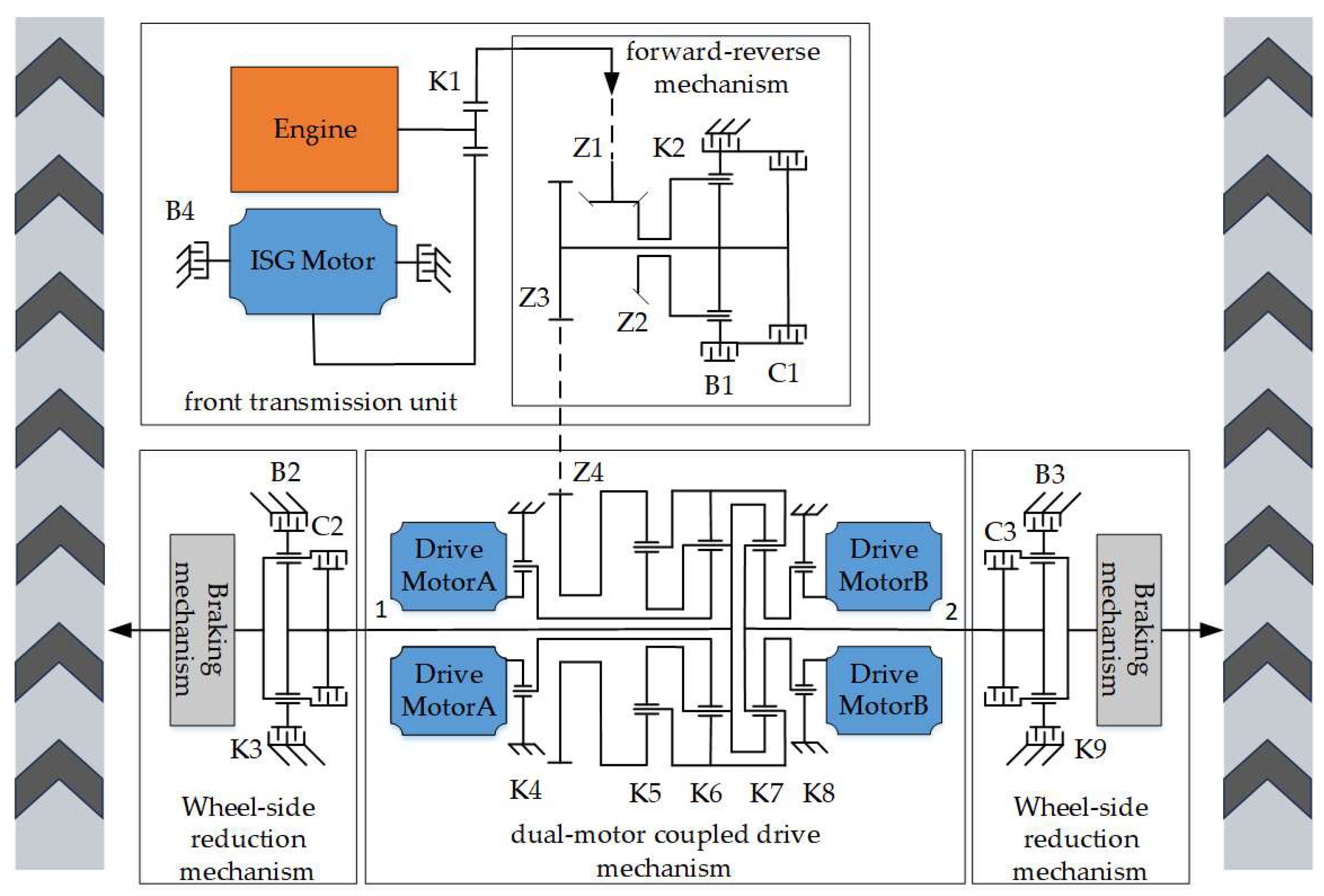
2.1. Introduction to System Scheme and Parameters

First, a dynamic model for the ECTS is established, which is divided into three parts: the front transmission unit, the dual-motor coupled drive mechanism (between Point 1 and Point 2), and the wheel-end reduction mechanism. The configuration of the ECTS is illustrated in Figure 1.

In Figure 1, the engine, Drive Motor A, and Drive Motor B provide power for the tracked vehicle, while the ISG motor assists in engine starting and generates electricity. The forward-reverse mechanism enables the tracked vehicle to run in reverse, and the coupling mechanism realizes torque superposition by coupling the power of the dual-side drive motors. The wheel-side reduction mechanism further reduces the rotational speed and increases the torque. Here, B1–B4 and C1–C3 are clutches, K1–K9 are planetary gear sets, and Z1–Z4 are transmission gears. $i_1$ represents the transmission ratio from the engine to the reversing mechanism, and $i_2$ represents the transmission ratio from the reversing mechanism to the planetary gears, where $i_1$ = 1 and $i_2$ = 8.5. The characteristic parameters of each planetary gear set are defined as $k_1$ = $k_3$ = $k_9$ = 2.478, $k_4$ = $k_8$ = 2.135, $k_5$ = 2, $k_6$ = $k_7$ = 2.2.

In the ECTS, the torque output by the engine is transmitted to both sides via the coupling mechanism with equal torque distribution, while the drive motors compensate for the difference between the target output torque of the two tracks and the torque provided by the engine. The engine and motors work in coordination to keep the engine operating within its high-efficiency range at all times, thereby reducing fuel consumption. The coupling mechanism enables power coupling of the dual-side drive motors and torque superposition, meeting the torque demands of scenarios such as heavy-load starting and hill climbing.

Specific parameters of the ECTS and tracked vehicle are listed as follows in

Table 1. Parameters of mechatronic composite transmission system and tracked vehicle.

Component	Parameter	Value
Engine	Maximum power	769.31 kW
	Maximum torque	1750 Nm
	Maximum rotational speed	4200 rpm
	Moment of inertia	2 kg·m2
ISG motor	Maximum power	550 kW
	Maximum torque	700 Nm
	Maximum rotational speed	20,000 rpm
	Moment of inertia	0.5 kg·m2
Drive motor	Maximum power	250 kW
	Maximum torque	3500 Nm
	Maximum rotational speed	2500 rpm
	Moment of inertia	4 kg·m2
Vehicle	Empty load mass	35,000 kg
	Wheel radius	0.318 m
	Friction resistance coefficient	0.06
	Air resistance coefficient	0.9
	Windward area	6 m2

.

2.2. ECTS Dynamic Model

Variables ${\mathrm{X}}_1$ and ${\mathrm{Y}}_1$ are defined as follows:

$$\begin{gathered} {\mathrm{X}}_1={\left[\begin{array}{cccc}{T}_E& T_{ISG}& {\ddot{\theta }}_Z^4& T_B^4\end{array}\right]}^{\mathrm{T}} \\ {\mathrm{Y}}_1={\left[\begin{array}{ccc}{\ddot{\theta }}_E& {\ddot{\theta }}_{ISG}& T_Z^4\end{array}\right]}^{\mathrm{T}} \end{gathered}$$

(1)

where $T_E$ is the engine torque, $T_{ISG}$ is the torque of the ISG motor, $T_B^4$ is the torque of the B4 clutch, $T_Z^4$ is the torque of the transmission gear Z4, ${\ddot{\theta }}_Z^4$ is the angular acceleration of the transmission gear Z4, ${\ddot{\theta }}_E$ is the angular acceleration of the engine, and ${\ddot{\theta }}_{ISG}$ is the angular acceleration of the ISG motor. Then, the dynamic model of the front transmission part can be derived as follows:

$${\mathrm{Y}}_1={{\mathrm{A}}_1}^{-1}{\mathrm{D}}_1{\mathrm{X}}_1$$

(2)

where the corresponding matrices are expressed in Equation (A1) of the Appendix A.

Similarly, variables ${\mathrm{X}}_3$ and ${\mathrm{Y}}_3$ are defined as follows:

$${\mathrm{X}}_3={\left[\begin{array}{ccccc}{T}_A& T_B& T_1& T_2& T_Z^4\end{array}\right]}^{\mathrm{T}}{\mathrm{Y}}_3={\left[\begin{array}{ccccc}{\ddot{\theta }}_A& {\ddot{\theta }}_B& {\ddot{\theta }}_1& {\ddot{\theta }}_2& {\ddot{\theta }}_Z^4\end{array}\right]}^{\mathrm{T}}$$

(3)

where $T_A$ is the torque of the left-hand drive motor A, $T_B$ is the torque of the right-hand drive motor B, $T_1$ is the torque at point 1, $T_2$ is the torque at point 2, ${\ddot{\theta }}_A$ is the angular acceleration of drive motor A, ${\ddot{\theta }}_B$ is the angular acceleration of drive motor B, ${\ddot{\theta }}_1$ is the angular acceleration at point 1, and ${\ddot{\theta }}_2$ is the angular acceleration at point 2. Then, the dynamic model of the dual-motor coupled drive mechanism (between points 1 and 2) is as follows:

$${\mathrm{Y}}_3={{\mathrm{A}}_3}^{-1}{\mathrm{D}}_3{\mathrm{X}}_3$$

(4)

where the corresponding matrices are expressed in Equations (A2) and (A3) of the Appendix A.

Similarly, variables ${\mathrm{X}}_7$ and ${\mathrm{Y}}_7$ are defined as follows:

$${\mathrm{X}}_7={\left[\begin{array}{cccc}{T}_{Cl}^2& T_B^2& {\ddot{\theta }}_1& {\ddot{\theta }}_O^L\end{array}\right]}^{\mathrm{T}}{\mathrm{Y}}_7={\left[\begin{array}{ccc}{T}_1& T_O^L& {\ddot{\theta }}_R^3\end{array}\right]}^{\mathrm{T}}$$

(5)

where $T_B^2$ is the torque of the B2 clutch, ${\ddot{\theta }}_O^L$ is the angular acceleration of the left-hand output, $T_O^L$ is the torque of the left-hand output, and ${\ddot{\theta }}_R^3$ is the angular acceleration of the ring gear of the third planetary gear set. Then, the dynamic model of the left-wheel-mounted reduction mechanism is as follows:

$${\mathrm{Y}}_7={{\mathrm{A}}_7}^{-1}{\mathrm{D}}_7{\mathrm{X}}_7$$

(6)

where the corresponding matrices are expressed in Equation (A4) of the Appendix A.

The dynamic model of the right-side wheel-mounted deceleration mechanism can be obtained in the same way:

$${\mathrm{Y}}_{11}={{\mathrm{A}}_{11}}^{-1}{\mathrm{D}}_{11}{\mathrm{X}}_{11}$$

(7)

ECTS has two main fault cases. (a) depicts the single-side drive motor fault case (taking the left motor failure as an example): when a single-side drive motor fails, the input torque of the faulty side motor is 0, and it stops participating in operation. (b) illustrates the electric drive system fault case: both left and right drive motors fail, and to prevent battery overcharging caused by continuous operation of the ISG motor, the ISG motor is locked once the starting process is complete, as shown in Figure 2.

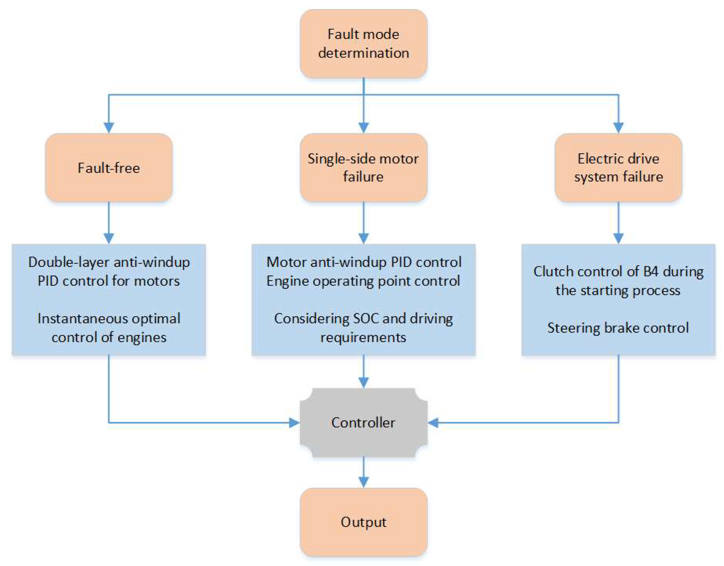
3. Fault-Tolerant Control

The fault-tolerant control of hybrid tracked vehicles is crucial for ensuring continuous operation under complex working conditions. In this section, a hierarchical control architecture is proposed:

• In the fault-free case, the dual-side drive motors optimize power distribution through an ID controller and achieve steering tracking by combining with an anti-windup PID algorithm [19,20,21], while the engine adopts an instantaneous optimal strategy to reduce fuel consumption.
• When a single-side drive motor fault occurs, only the non-faulty side participates in steering drive. Engine power is dynamically adjusted based on the SOC to balance battery charging/discharging and driving demands.
• When an electric drive system fault occurs, the engine drives the tracked vehicle independently. The load is controlled via the B4 clutch and mechanical steering can be achieved by leveraging the brake pressure difference.

3.1. Control Strategy in Fault-Free Case

A control strategy for the dual-side drive motors is proposed for straight driving and steering conditions of tracked vehicles under the fault-free case. Based on the relationship between torque, rotational speed, and power, the target output power is calculated from the target output torques on both sides. Taking the output power of the power battery as feedback, an ID controller is designed to calculate the engine power, and an instantaneous optimal strategy is adopted to control the operating point of the engine. At the same time, the drive motors compensate for the difference between the target output torques on both sides of the track and the torques provided by the engine.

During straight-line driving, the relationships between the target torque of the drive motor, the actual torque of the engine, and the target torque of the output shaft are given in Equation (A5) of Appendix B.

During the steering process, the target steering angle is tracked. A double-layer anti-windup PID algorithm is designed for the dual-side drive motors. The design details of the anti-windup PID control algorithm can be found in Equations (A6)–(A8) of Appendix B. According to the difference between the actual output rotational speeds and the target output rotational speeds of the driving wheels on both sides, the difference in the output torques of the dual-side drive motors is controlled. In the outer loop, the target steering angular velocity is provided through a PID controller according to the difference in the heading angles:

$$Y_{omega}^{cmd,PID}=f\left(e_{Yaw},{\mathrm{e}}_{\mathrm{int}}\right)$$

(8)

$$e_{\mathrm{int}}=g\left(e_{Yaw}\right)$$

(9)

where $e_{Yaw}$ is the difference between the target heading angle and the actual heading angle of the vehicle, and $Y_{omega}^{cmd,PID}$ is the target angular velocity of the vehicle.

In the inner loop, the steering torque is calculated based on the angular velocity difference:

$$T_{DM}^{cmd,PID}=f\left(e_{\omega },{\mathrm{e}}_{\mathrm{int}}\right)$$

(10)

$$e_{\mathrm{int}}=g\left(e_{\omega }\right)$$

(11)

where $e_{\omega }$ is the difference between the target angular velocity and the actual angular velocity of the vehicle, and $T_{DM}^{cmd,PID}$ is the difference in the torques of the drive motors.

To improve the endurance of the tracked vehicle, after determining the target power of the engine, it is necessary to dynamically set the operating point of the engine according to the current working state of the system. Based on the instantaneous optimal strategy, the instantaneous optimal operating point of the engine is calculated by traversing and computing the vehicle speed and the required power. Under certain vehicle speed and engine rotational speed conditions, the relationship between the engine fuel consumption rate and the engine fuel consumption power can be obtained as follows:

$$P_{EngFul}={\displaystyle \frac{34000{\eta }_{EngFul}}{1000}}$$

(12)

where ${\eta }_{EngFul}$ is the engine fuel consumption rate, and $P_{EngFul}$ is the engine fuel consumption power.

The target output power of the engine is calculated by considering the power battery SOC target and required power while taking into account the efficiency characteristics of the ISG motor, drive motor, and engine. Based on the instantaneous optimal method, the target power of the engine and the ring gear speed of planetary carrier 1 are calculated under different vehicle speeds, drive demand power, and battery charging power. The maximum engine speed is further derived via look-up tables to keep the engine operating at its optimal point. The scatter plot of engine operating points is shown in Figure 3.

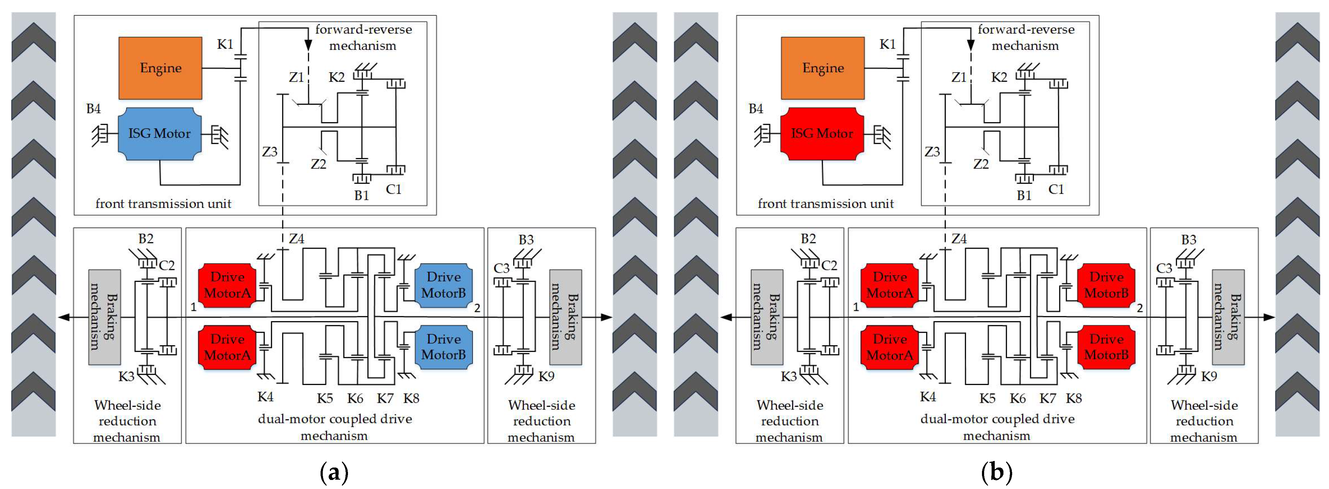
3.2. Control Strategy in the Case of Single-Side Drive Motor Fault

When a single-side drive motor malfunctions, the input torque of the faulty motor becomes 0, and it stops working. If the non-faulty drive motor participates in straight-line driving, it will cause a speed difference. Therefore, the non-faulty drive motor only participates in driving during the steering process. The target rotational speeds of the tracks on both sides are calculated based on the target vehicle speed and the target heading angle. The motor torque required for steering is used as the input of the PID controller, and the actual motor torque serves as the system feedback to assist the engine in completing the steering. An anti-windup PID control is applied to the non-faulty motor.

To prevent the power battery from being overcharged due to the power output of the engine after being split, it is necessary to control the engine operating point by taking into account the SOC and the driving demand. The engine needs to adjust its operating point according to the current SOC of the battery to ensure that the battery can operate efficiently at different charge levels. The relationship between the battery power and the engine power is provided as follows:

$$P_{\mathrm{E}}=P_{Out}+P_{\mathrm{Battery}}$$

(13)

where $P_{\mathrm{E}}$ is the engine power, $P_{Out}$ is the output shaft power, and $P_{\mathrm{Battery}}$ is the battery power.

A constant SOC value is set, and the engine power is adjusted by utilizing the relationship between the battery power and the engine power. When the SOC of the battery is too low, the battery should be kept near the constant SOC value. According to the current engine power and the vehicle speed, the target rotational speed of the engine is decreased to increase the rotational speed of the ISG motor. The battery is then charged to maintain high dynamic performance. When the SOC of the battery is relatively high, the target rotational speed of the engine is increased, and the engine operating point is raised to protect the battery.

3.3. Control Strategy in the Case of Electric Drive System Fault

In the event of simultaneous failures of both drive motors, the vehicle will be powered solely by the engine. To prevent the battery from being overcharged due to the continuous operation of the ISG motor, the ISG motor is locked after the vehicle starts. The engine speed and the vehicle speed gradually change from a decoupled state to a coupled state. It is necessary to control the steering brake to achieve variable-radius steering of the vehicle. A map illustrating the relationship between fuel consumption rate and engine output speed and torque is derived via interpolation. As shown in the engine external characteristic curve in Figure 4, if the engine is required to deliver high torque during startup, it must operate at a relatively high speed. Additionally, the fuel consumption rate tends to be lower when both engine speed and torque are higher.

Therefore, when the vehicle starts, the requirements for the engine speed are expressed as follows:

$$n_{e,cmd}=f\left(\min \left(T_{e,\max },T_{e,cmd}\right)\right)$$

(14)

where $n_{e,cmd}$ is the target rotational speed of the engine, $T_{e,\max }$ represents the maximum output torque of the engine, and $T_{e,cmd}$ represents the target torque of the engine.

To achieve power transmission during the starting process under the electric drive system fault conditions while maintaining precise engine speed regulation, an anti-windup PID controller is designed for the B4 clutch to control the engagement pressure. Furthermore, the magnitude of the torque transmitted by the B4 clutch is controlled so as to realize the control of the engine load and the power transmission during starting.

Under the coupled working condition of straight driving and steering after the vehicle has completed the starting process, the engine alone provides the driving torque. Meanwhile, the brakes of the driving wheels on both sides are used to realize the steering function of the vehicle. The pressure design for the left and right brakes is shown in Equation (A9) of Appendix B.

The control outputs of the brakes on both sides can be normalized as follows:

$$P_{brake}=\max \left(-P_{brake,\max },\min \left(P_{brake,\max },\left(k_{p}e+\min \left(I_{\min },\max \left(I_{\max },k_i{\displaystyle \int {\mathrm{e}}_{\mathrm{int}}dt}\right)\right)+k_{p}e\right)\right)\right)$$

(15)

Finally, the target heading angle is calculated according to the target vehicle speed, the target rotational speeds of the tracks on both sides, and the vehicle degree-of-freedom model. An anti-windup PID controller is designed for the brakes to control the engagement pressure of the brakes.

The overall flow chart of ECTS fault-tolerant control is shown in Figure 5.

4. Simulation Verification

In this section, the numerical simulations are provided to verify the driving performance of the tracked vehicle under different fault scenarios. First, two working conditions are chosen for three different fault scenarios of the ECTS, namely, straight driving and steering. The three fault scenarios include the normal operation state of the electric drive system, the fault case of a single-side drive motor, and the extreme scenario of the fault case of the electric drive system. Through the comparative analysis of the vehicle speed and the vehicle heading angle, the effectiveness of the designed fault-tolerant control strategy for the tracked vehicle is evaluated.

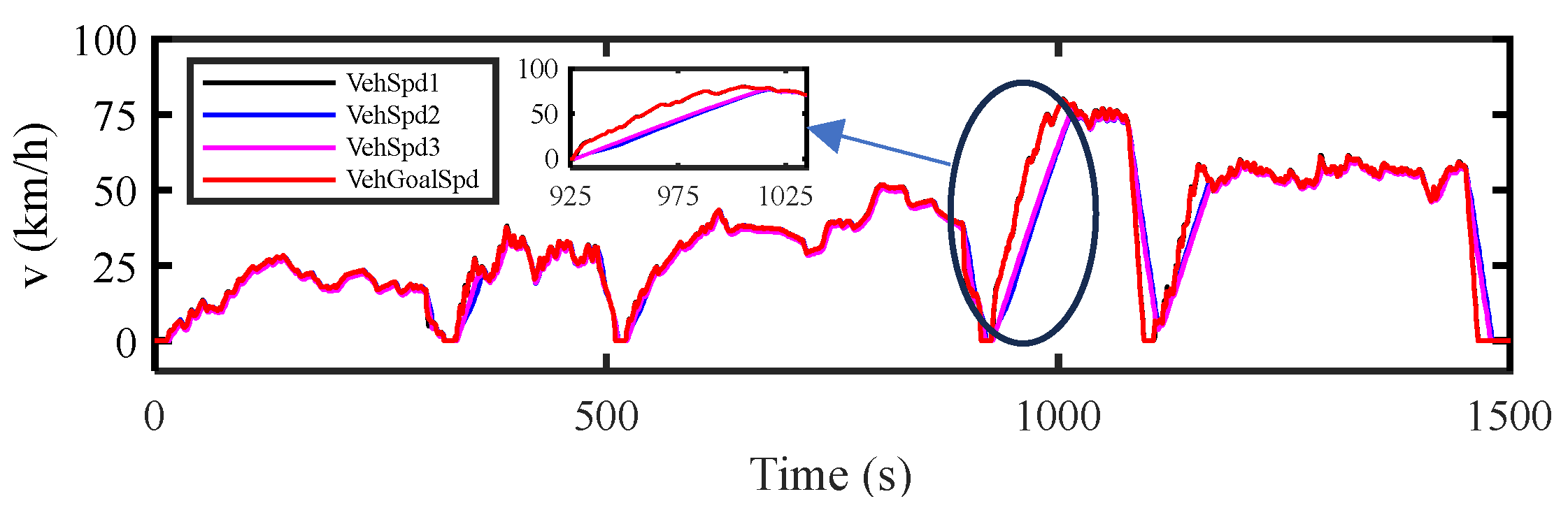
4.1. Analysis of Straight-Line Driving Conditions

4.1.1. Comparison of Straight-Line Driving Conditions

Figure 6 shows the vehicle speed change curves of the tracked vehicle during straight-line driving according to the preset speed cycle under three fault conditions where VehGoalSpd represents the target vehicle speed, VehSpd1 represents the vehicle speed in the fault-free case, VehSpd2 represents the vehicle speed in the single-motor fault case, and VehSpd3 represents the vehicle speed in the electric drive system fault case. As shown in Figure 6, the vehicle can achieve stable straight-line driving according to the preset speed cycle requirements of the tracked vehicle. The three actual vehicle speeds are highly consistent with the target speeds, indicating that the tracked vehicle can still accurately respond to driving demands during straight-line driving under fault conditions, with good dynamic adjustment capability of the power system.

In the fault case of the electric drive system, the ISG motor is locked after the vehicle has completed the starting process. The torque and speed of the ISG motor are shown in Figure 7. As observed in Figure 7, the ISG motor generates torque when assisting the engine start, and its torque drops to zero after being locked by the B4 clutch.

The engagement curve of the B4 clutch under the straight driving working condition in the fault case of the electric drive system. The torque variation of the B4 clutch is shown in Figure 8. From Figure 8, it can be found that the B4 clutch regulates the torque to bring the engine into a feasible speed range.

4.1.2. Straight-Run Failure Condition

In the straight-driving condition of the tracked vehicle, the throttle opening is set as 0.6, and the motor failure was triggered at 15 s during the acceleration process. Figure 9 shows the speed change diagram of the tracked vehicle during the acceleration process. VehSpd1 represents the speed change of the tracked vehicle in the fault-free case, VehSpd2 represents the speed change of the single-side drive motor fault case, and VehSpd3 represents the speed change of the electric drive system fault case. In this paper, the maximum speed that the tracked vehicle can reach at the 30 s and the acceleration of the tracked vehicle at 30 s are used as the evaluation criteria for the vehicle’s dynamic performance. The maximum speed variations of the tracked vehicle are shown in

Table 2. Variation in the maximum speed of the tracked vehicle.

Model	Parameter	Value
Fault-free	Maximum vehicle speed	95.3 km/h
	Final acceleration	0.14 m/s2
Single-side motor failure	Maximum vehicle speed	63.5 km/h
	Final acceleration	0.05 m/s2
	Degree of decline in dynamic performance	33.37%
Electric drive system failure	Maximum vehicle speed	53.5 km/h
	Final acceleration	−0.12 m/s2
	Degree of decline in dynamic performance	43.86%

.

4.2. Analysis of Steering Driving Conditions

Figure 10 shows the comparison of vehicle speeds in different fault cases under the steering working condition. SteerVehGoalSpd represents the target steering vehicle speed. VehSpd1 represents the vehicle speed change of the tracked vehicle in the fault-free case, VehSpd2 represents the vehicle speed change of the single-side drive motor fault case, and VehSpd3 represents the vehicle speed change of the electric drive system fault case. From Figure 10, it can be seen that both the fault-free case and the single-motor fault case meet the preset speed requirements. In the case of dual-motor faults, there is a slight deviation between the final speed and the preset speed, but this does not affect the normal steering of the tracked vehicle. This indicates that the tracked vehicle can normally meet the steering and driving requirements under all three fault scenarios mentioned above.

Figure 11 presents a comparison of the variations in the vehicle heading angles of the tracked vehicle under the steering working condition among the fault-free mode and the two fault modes. In Figure 11, the symbols Simulate angle 1, Simulate angle 2 and Simulate angle 3 represent the variation in the heading angle in the fault-free mode, single-side drive motor fault mode, and electric drive system fault mode, respectively. This allows for a more intuitive observation of the changes in the steering speed of the vehicle under different fault modes. From Figure 11, it can be seen that the tracked vehicle’s heading angles met the preset requirements under three fault cases and changed smoothly, which implies that the tracked vehicle can smoothly fulfill the steering requirements in all three fault cases.

Since the drive motors on both sides of the tracked vehicle fail and cannot assist the vehicle in steering, the steering braking mechanisms on the left and right sides engage to generate torque. This creates a difference in the rotational speeds of the tracks on the left and right sides of the vehicle, thereby enabling the tracked vehicle to complete the steering maneuver. The torque of the steering brakes on the left and right sides are shown in Figure 12. It is observed from Figure 12 that the torque variations of the left and right steering brakes are inconsistent, which leads to different resistances on the two tracks and thus forms a steering moment to make the tracked vehicle steer.

5. Conclusions

This study addresses the fault issues of the ECTS in tracked vehicles by proposing a multi-mode fault-tolerant control strategy and verifying its effectiveness. Through establishing a system dynamics model, a control scheme based on the anti-windup PID algorithm is designed: the dual-layer anti-windup PID control for motors combined with the instantaneous optimal control method for the engine is adopted under fault-free conditions; the anti-windup PID control for the motor and the coordinated SOC-drive control method are implemented in the case of single-motor failure; and the joint control method of the clutch and steering brake is activated during electric drive failure. Simulations show that the system can maintain basic driving functions under all three states, but the power performance declines in fault states: the straight-line driving power decreases by 33.37% under single-motor fault, and the decline reaches 43.86% during electric drive failure. This research provides a theoretical basis for the fault-tolerant control of tracked transmission systems under complex working conditions.

The current research has not conducted an in-depth exploration on the real-time performance and accuracy of fault diagnosis, making it difficult to cope with complex and ever-changing actual fault conditions. In future research, we will continue to explore the fault detection of the ECTS in tracked vehicles and the impacts of different fault conditions on various aspects of the vehicle. This may provide a reference for other researchers to more accurately assess and address the fault issues of tracked vehicle drive systems.

References

1. Qie, T.; Wang, W.; Yang, C.; Yang, C. A heavy-duty tracked vehicle model with a reduced feasible domain for motion tracking control considering dynamic characters of hybrid powertrain. Adv. Eng. Inform. 2024, 62, 102760. [Google Scholar] [CrossRef]
2. Milićević, S.; Blagojević, I.; Milojević, S.; Bukvić, M.; Stojanović, B. Numerical analysis of optimal hybridization in parallel hybrid electric powertrains for tracked vehicles. Energies 2024, 17, 3531. [Google Scholar] [CrossRef]
3. Li, R.; Fan, J.; Han, Z.; Guan, S.; Qin, Z. Configuration design and control of hybrid tracked vehicle with three planetary gear sets. J. Cent. South Univ. 2021, 28, 2105–2119. [Google Scholar] [CrossRef]
4. Tan, Y.; Xu, J.; Ma, J.; Li, Z.; Chen, H.; Xi, J.; Liu, H. A transferable perception-guided EMS for series hybrid electric unmanned tracked vehicles. Energy 2024, 306, 132367. [Google Scholar] [CrossRef]
5. Han, Z.; Liang, X.; Zhang, W.; Liu, Y.; Liu, J. Dynamic characterization and vibration response optimization of EMT system for tracked vehicles. Sci. Rep. 2025, 15, 12614. [Google Scholar] [CrossRef] [PubMed]
6. Randive, V.; Subramanian, S.C.; Thondiyath, A. Component sizing of single and dual drive series hybrid electric powertrain for military tracked vehicles. In Proceedings of the IEEE Vehicle Power and Propulsion Conference (VPPC), Hanoi, Vietnam, 14–17 October 2019; IEEE: New York, NY, USA, 2019. [Google Scholar]
7. Djeziri, M.A.; Merzouki, R.; Bouamama, B.O.; Ouladsine, M. Fault diagnosis and fault-tolerant control of an electric vehicle overactuated. IEEE. Trans. Veh. Technol. 2012, 62, 986–994. [Google Scholar] [CrossRef]
8. Richter, J.H.; Weiland, S.; Heemels, W.P.M.H.; Lunze, J. Decoupling-based reconfigurable control of linear systems after actuator faults. In Proceedings of the European Control Conference (ECC), Budapest, Hungary, 23–25 August 2009; IEEE: New York, NY, USA, 2009. [Google Scholar]
9. Zhang, L.P.; Gong, D.L. Passive fault-tolerant control for vehicle active suspension system based on H2/H∞ approach. J. Vibroeng. 2018, 20, 1828–1849. [Google Scholar] [CrossRef]
10. Zuñiga, M.A.; Ramírez, L.A.; Romero, G.; Alcorta-García, E.; Arceo, A. Passive fault-tolerant control of a 2-DOF robotic helicopter. Information 2021, 12, 445. [Google Scholar] [CrossRef]
11. Indriawati, K.; Kurnianingtyas, R. Real-time implementation of passive fault-tolerant speed control for unloading MS150 DC motor system. In Proceedings of the E3S Web of Conferences, Pekanbaru, Indonesia, 23 September 2020; EDP Sciences: Les Ulis, France, 2020. [Google Scholar]
12. Hou, Z.; Lee, C.K.M.; Lv, Y.; Keung, K.L. Fault detection and diagnosis of air brake system: A systematic review. J. Manuf. Syst. 2023, 71, 34–58. [Google Scholar] [CrossRef]
13. Khaneghah, M.Z.; Alzayed, M.; Chaoui, H. Fault detection and diagnosis of the electric motor drive and battery system of electric vehicles. Machines 2023, 11, 713. [Google Scholar] [CrossRef]
14. Abdoune, F.; Nouiri, M.; Cardin, O.; Castagna, P. An enhanced methodology of fault detection and diagnosis based on digital twin. IFAC-PapersOnLine 2022, 55, 43–48. [Google Scholar] [CrossRef]
15. Qi, B.; Yang, L.; Zhang, L.; Zhang, R. Adaptive fault-tolerant control during the mode switching for electric vehicle dual-mode coupling drive system. Automot. Innov. 2021, 4, 56–69. [Google Scholar] [CrossRef]
16. Guo, M.; Bao, C.; Cao, Q.; Xu, F.; Miao, X.; Wu, J. Fault-tolerant control study of four-wheel independent drive electric vehicles based on drive actuator faults. Machines 2024, 12, 450. [Google Scholar] [CrossRef]
17. Zhou, Z.; Chen, M.; Zhang, G.; Shen, W.; Yang, R. Research on active fault tolerant control strategy for distributed drive electric vehicles based on multi-actuator failure. Eng. Lett. 2025, 33, 123–135. [Google Scholar]
18. Zhou, Z.; Zhang, G.; Chen, M. A fault-tolerant control strategy for distributed drive electric vehicles based on model reference adaptive control. Actuators 2024, 13, 486. [Google Scholar] [CrossRef]
19. Hernandez-Barragan, J.; Rios, J.D.; Alanis, A.Y.; Lopez-Franco, C.; Gomez-Avila, J.; Arana-Daniel, N. Adaptive single neuron anti-windup PID controller based on the extended kalman filter algorithm. Electronics 2020, 9, 636. [Google Scholar] [CrossRef]
20. Huang, J.; Wang, J.; Fang, H. An anti-windup self-tuning fuzzy PID controller for speed control of brushless DC motor. Automatika 2017, 58, 321–335. [Google Scholar]
21. Tahoun, A.H. Anti-windup adaptive PID control design for a class of uncertain chaotic systems with input saturation. ISA Trans. 2017, 66, 176–184. [Google Scholar] [CrossRef] [PubMed]
Figure 1. ECTS configuration.
Machines 13 00622 g001
Figure 2. Schematic diagram of the fault scenario. (a) Single-side drive motor fault case; (b) electric drive system fault case.
Machines 13 00622 g002
Figure 3. Scatter diagram of the engine operating points.
Machines 13 00622 g003
Figure 4. Engine external characteristic curve diagram.
Machines 13 00622 g004
Figure 5. Flowchart of ECTS fault-tolerant control strategies.
Machines 13 00622 g005
Figure 6. Target vehicle speed and vehicle speeds for the three fault modes.
Machines 13 00622 g006
Figure 7. Rotational speed and torque of the ISG motor under electric drive system fault case.
Machines 13 00622 g007
Figure 8. Engagement state of the B4 clutch under electric drive system fault case.
Machines 13 00622 g008
Figure 9. The vehicle speed under different faults during normal straight-line driving conditions.
Machines 13 00622 g009
Figure 10. Speed comparison under the three fault scenarios during the steering working condition.
Machines 13 00622 g010
Figure 11. Comparison of vehicle heading angles.
Machines 13 00622 g011
Figure 12. The torque of the steering brake.
Machines 13 00622 g012