Dynamic Positioning and Optimization of Magnetic Target Based on Binocular Vision

Abstract

Aiming at the problems of visual occlusion, reduced positioning accuracy and pose loss in the dynamic scanning process of aviation large components, this paper proposes a binocular vision dynamic positioning method based on magnetic target. This method detects the spatial coordinates of the magnetic target in real time through the binocular camera, extracts the target center to construct a unified reference system of the measurement platform, and uses MATLAB simulation to analyze the influence of different target layouts on the scanning stability and positioning accuracy. On this basis, a dual-objective optimization model with the objectives of ‘minimizing the number of targets’ and ‘spatial distribution uniformity’ is established, and Monte Carlo simulation is used to evaluate the robustness under Gaussian noise and random frame loss interference. The experimental results on the C-Track optical tracking platform show that the optimized magnetic target layout reduces the rotation error of the dynamic scanning from 0.055° to 0.035°, the translation error from 0.31 mm to 0.162 mm, and the scanning efficiency is increased by 33%, which significantly improves the positioning accuracy and tracking stability of the system under complex working conditions. This method provides an effective solution for high-precision dynamic measurement of aviation large components.

1. Introduction

Binocular vision [1] technology is widely used in high-end equipment manufacturing as an important means to achieve high-precision three-dimensional shape detection. However, the traditional method generally relies on the reflective marker points pasted on the surface of the workpiece for pose tracking, which has significant limitations [2]. On the one hand, the pasting process of the marker points will destroy the surface integrity of the workpiece; on the other hand, in the measurement process, the marker points are easily unable to be captured due to visual occlusion, resulting in inaccurate pose tracking, thereby reducing the full-size detection accuracy of complex curved parts. In contrast, the magnetic attraction target is a movable target with reflective markers. Through the binocular vision positioning technology of the optical tracker, it can accurately and real-time determine the pose of the posture adjustment platform during the movement process. It can effectively replace the method of pasting reflective markers on the surface of the workpiece, significantly improving the pose tracking accuracy and point cloud integrity, and providing a new measurement theory and technical support for the field of precision manufacturing.

In binocular vision-based geometric model localization [3,4], a key step is to scan the target multiple times and register the resulting point clouds into a complete 3D point cloud model [5]. The main tasks of geometric model reconstruction include point cloud registration and model construction [6]. In point cloud localization, registration can generally be performed based on the object itself or its key edge features [7]. However, object-based localization involves considerable manual operations, which are subjective and error-prone. Therefore, current research focuses more on (semi-)automated point cloud localization methods based on features such as key points and curves [7]. In addition, 3D point cloud models can also be constructed using 2D image sets of the target combined with reconstruction algorithms [8]. Some studies have integrated binocular vision with images or video [9] to improve the accuracy of spatial pose estimation in geometric model localization [10]. Research on 3D scan-based localization and field-of-view analysis mainly focuses on acquiring depth information from the surface of the measured object or determining its position based on 2D image coordinates [11]. For example, Barazzetti [12] proposed a novel semi-automated method based on laser scanning and photogrammetry for generating 3D parametric as-built models from point clouds. NURBS curves and surfaces were used to reconstruct complex and irregular objects without excessively simplifying the information embedded in large-scale point clouds, ensuring that the resulting models remain useful for practical applications and productive work. Bopaya Bidanda [13] and colleagues investigated geometric and spatial factors that may affect scanning variance. This functional relationship was modeled using a Bayesian extreme learning framework, which was later applied to determine the optimal object pose for minimizing variance. A Bayesian optimization strategy was introduced to solve this localization minimization problem. Tingcheng Li [14] introduced a machine learning-based method capable of accurately predicting the 3D coverage of parts based on scanning configurations provided as input. This enables pre-scan estimation of which regions of a part will be effectively captured, marking a paradigm shift from theoretical visibility metrics to data-driven rules learned from real-world conditions. Li [15] proposed a spatial localization method for kiwifruit using binocular cameras and deep learning-based stereo imaging. Based on detected fruits and their depth information, this method utilizes stereo vision principles to accurately predict the 3D spatial coordinates of small and densely packed kiwifruits in complex background environments. However, traditional binocular vision localization methods remain limited in flexibility [16]. During scanning, frame losses of the scanning head and platform may result in incomplete point cloud acquisition, compromising the timeliness of pose tracking. Therefore, there is an urgent need to develop a dynamic localization method suited for dynamic scanning environments. Such a method would improve the field-of-view threshold of optical trackers and offer an effective solution for dynamic measurement of large aerospace components.

Based on the above research, this study proposes a binocular vision-based dynamic localization method using magnetic targets. The method is developed based on the spatial localization principle of magnetic targets. A unified coordinate framework is first established, including the coordinate systems of the workpiece, the scanner, and the platform, which defines the overall dynamic scanning process and the transformation relationships among all components. A precise mapping model from the pixel coordinate system to the world coordinate system is constructed based on binocular vision principles, enabling accurate spatial localization of magnetic targets mounted on the six-degree-of-freedom adjustment platform. On this basis, the NSGA-II multi-objective optimization algorithm is introduced to optimize the layout of magnetic targets with the objectives of minimizing the number of targets and maximizing spatial coverage. This ensures that at least four non-coplanar targets remain visible to the optical tracker throughout the platform’s motion, significantly improving the robustness and accuracy of pose estimation. Simulation and experimental results quantitatively compare localization performance with and without optimization, demonstrating the effectiveness and stability of the proposed method in complex dynamic scanning environments. The results show that this method effectively enhances localization accuracy and reliability in the measurement of complex components such as aero-engine casings, providing a solid theoretical foundation and practical guidance for dynamic scanning of large-scale aerospace parts.

2. Principle of Target Spatial Localization

2.1. Principle of Target Localization

The role of the magnetic target is to locate the real-time pose parameters of the investment platform during the movement through the binocular vision imaging principle of the optical tracker. Binocular vision is to obtain image information through two cameras, calculate the parallax, so that the computer can perceive the three-dimensional world [17]. The principal diagram of the binocular stereo vision system to locate the spatial coordinate position of the target is shown in Figure 1a. The two cameras of the C-Track collect and locate the target at the same time, and the target position and its environment can be determined by triangulation, as shown in Figure 1b.

The distance between the projection centers of the two cameras is denoted as b, also known as the baseline. An arbitrary point P in 3D space is projected onto the left and right image planes as P_L and P_R, respectively. According to the principle of the rectilinear propagation of light, point P in 3D space lies at the intersection of the lines connecting each camera’s projection center with its corresponding image point. Let P_L and P_R represent the distances from the image points to the left and right imaging planes, respectively. The disparity d between the left and right views of point P can be defined as follows:

$$d=\left|x_L-x_R\right|$$

(1)

The distance between the two image points is given by

$$P_L{P}_R=b-\left(x_L-{\displaystyle \frac{L}{2}}\right)-\left({\displaystyle \frac{L}{2}}-x_R\right)=b-\left(x_L-x_R\right)$$

(2)

According to the principles of triangulation, it can be derived that

$${\displaystyle \frac{b-\left(x_L-x_R\right)}{z-f}}={\displaystyle \frac{b}{z}}$$

(3)

The distance z from target point p to the projection center plane is given by

$$z={\displaystyle \frac{bf}{x_L-x_R}}$$

(4)

(1)

Relationship between the image coordinate system and the camera coordinate system

The relationship between the image coordinate system and the camera coordinate system can be derived from two similar triangles, as shown in Equation (5) and illustrated in Figure 2.

$$\left\{\begin{array}{l}x={\displaystyle \frac{f{X}_c}{Z_c}}\\ y={\displaystyle \frac{f{Y}_c}{Z_c}}\end{array}\right.$$

(5)

The transformation into a homogeneous matrix is given by

$$\left[\begin{array}{l}x\\ y\\ z\end{array}\right]={\displaystyle \frac{1}{Z_c}}\left[\begin{array}{c}f\\ 0\\ 0\end{array}\begin{array}{c}0\\ f\\ 0\end{array}\begin{array}{c}0\\ 0\\ 1\end{array}\begin{array}{c}0\\ 0\\ 0\end{array}\right]\left[\begin{array}{c}{X}_C\\ Y_C\\ Z_C\\ 1\end{array}\right]$$

(6)

In Equation (6), f represents the focal length of the camera, (Xc, Yc, Zc) denote the coordinates of a 3D point in the camera coordinate system, and the projection is modeled using a perspective projection matrix followed by homogeneous normalization.

(2)

Relationship between the pixel coordinate system and the image coordinate system

The relationship between the pixel coordinate system and the image coordinate system involves a scaling factor and a translation of the origin. Assuming that the pixel coordinates are scaled by ${\displaystyle \frac{1}{dx}}$ along the u-axis and by ${\displaystyle \frac{1}{dy}}$ along the v-axis, the transformation can be represented as shown in Figure 3.

In general, the two axes of the pixel coordinate system and the image coordinate system are not orthogonal to each other. The relationship between the camera coordinate system and the pixel coordinate system can therefore be obtained by combining their respective transformations, as shown in the following Equation (7):

$$Z_C\left[\begin{array}{c}u\\ v\\ 1\end{array}\right]=\left[\begin{array}{ccc}{\displaystyle \frac{1}{dx}}& 0& u_0\\ 0& {\displaystyle \frac{1}{dy}}& v_0\\ 0& 0& 1\end{array}\right]\left[\begin{array}{cccc}f& 0& 0& 0\\ 0& f& 0& 0\\ 0& 0& 1& 0\end{array}\right]\left[\begin{array}{c}{X}_C\\ Y_C\\ Z_C\\ 1\end{array}\right]$$

(7)

(3)

Relationship between the camera coordinate system and the world coordinate system

The transformation from the camera coordinate system to the world coordinate system involves only a pose transformation, as illustrated in Figure 4. The matrix form is given as follows in Equation (8):

$$\left[\begin{array}{c}{X}_C\\ Y_C\\ Z_C\\ 1\end{array}\right]=\left[\begin{array}{cc}R& T\\ 0& 1\end{array}\right]\left[\begin{array}{c}{X}_W\\ Y_W\\ Z_W\\ 1\end{array}\right]$$

(8)

The transformation relationships among the four coordinate systems are illustrated in Figure 5, and the final transformation result is given in Equation (9).

$$Z_c=\left[\begin{array}{l}u\\ v\\ 1\end{array}\right]=\left[\begin{array}{ccc}{\displaystyle \frac{1}{dx}}& \gamma & u_0\\ 0& {\displaystyle \frac{1}{dy}}& v_0\\ 0& 0& 1\end{array}\right]\left[\begin{array}{ccc}f& 0& 0\\ 0& f& 0\\ 0& 0& 1\end{array}\right]\left[\begin{array}{cc}R& T\\ 0^T& 1\end{array}\right]\left[\begin{array}{c}{X}_W\\ Y_W\\ Z_W\\ 1\end{array}\right]$$

(9)

2.2. Establishment of Target Coordinate Systems

The spatial localization of magnetic targets plays a critical role in determining the positioning accuracy of the six-degree-of-freedom platform and the corresponding workpiece. Throughout the measurement field of view, it is essential to ensure that the number of magnetic targets tracked by the optical tracker remains greater than four. This prevents pose loss and large-scale point cloud omissions during the scanning process. In rigid body localization [18], three non-collinear targets are typically selected to construct a local coordinate system. The three axes are defined according to the right-hand rule, using one of the targets as the origin. This approach ensures that the constructed coordinate system satisfies the orthogonality requirement of rigid body transformations. For systems with multiple magnetic targets, a central point can be introduced as the reference origin of the global coordinate system to define the overall platform pose, thereby enabling consistent spatial representation.

Assuming there are n targets (n ≥ 4) within the measurement field of view, the spatial position of each target can be expressed as

$$p_i=\left(x_i,y_i,z_i\right)(i=1,2,3,\cdots ,n)$$

(10)

The steps for establishing the coordinate system are shown in Figure 6:

In Figure 6:

Step 1: Select a point P₁ in the magnetic target as the origin and link P₂, as shown in Figure 7:

Step 2: Select three additional non-collinear points, as shown in Figure 8, and compute the corresponding vectors.

$$\begin{array}{l}{V}_1=p_2-p_1=\left(x_2-x_1,y_2-y_1,z_2-z_1\right)\\ V_2=p_3-p_1=\left(x_3-x_1,y_3-y_1,z_3-z_1\right)\\ V_3=p_4-p_1=\left(x_4-x_1,y_4-y_1,z_4-z_1\right)\end{array}$$

(11)

Step 3: Compute the cross product of vectors V₁ and V₂ to obtain vector n:

$$n=V_1\times V_2$$

(12)

Step 4: Normalize vectors V₁ and V₂, and construct the rotation matrix R:

$$R=\left[\begin{array}{ccc}{\displaystyle \frac{v_{1x}}{‖v_1‖}}& {\displaystyle \frac{v_{2x}}{‖v_2‖}}& {\displaystyle \frac{n_x}{‖n‖}}\\ {\displaystyle \frac{v_{1y}}{‖v_1‖}}& {\displaystyle \frac{v_{2y}}{‖v_2‖}}& {\displaystyle \frac{n_y}{‖n‖}}\\ {\displaystyle \frac{v_{1z}}{‖v_1‖}}& {\displaystyle \frac{v_{2z}}{‖v_2‖}}& {\displaystyle \frac{n_z}{‖n‖}}\end{array}\right]$$

(13)

Based on the above principle, the spatial coordinate system of multiple magnetic targets can be established, allowing the calculation of the centroid of the target group. The center coordinate system of multiple groups of magnetic targets can be determined using the following Equation (14):

$$C=\left({\displaystyle \frac{1}{n}}\sum _{i=1}^n{x}_i,{\displaystyle \frac{1}{n}}\sum _{i=1}^n{y}_i,{\displaystyle \frac{1}{n}}\sum _{i=1}^n{z}_i\right)$$

(14)

Select two base points as basis vectors for the calculation:

$$\begin{array}{l}{V}_1=P_2-C=(x_2-C_x,y_2-C_y,z_2-C_z)\\ V_2=P_1-C=(x_1-C_x,y_1-C_y,z_1-C_z)\end{array}$$

(15)

Obtain the normal vector by computing the cross product of vectors V₁ and V₂:

$$n^{\prime }=V_1\times V_2$$

(16)

Transform the spatial coordinates of all magnetic targets into a coordinate system with point C as the origin:

$$P_i^{\prime }=R(P_i-C)$$

(17)

The final result obtained from the above equation represents the coordinates in the central coordinate system formed by the combination of multiple magnetic targets.

2.3. Coordinate System Simulation Verification

To verify the feasibility of the proposed center coordinate system construction method based on magnetic targets, a corresponding MATLAB (r2022a) simulation was conducted. Six magnetic targets were selected in 3D space to simulate their uniform distribution on the surface of a six-degree-of-freedom platform, and their spatial coordinates in the world coordinate system were defined as follows: [250,0,600], [0,300,610], [−250,0,590], [0,−300,605], [220,220,580], [−220,−220,605]. (unit: mm). All target data were defined in the MATLAB R2022a environment without introducing any random disturbance, ensuring full reproducibility of the process.

Subsequently, the geometric centroid of all targets was calculated and taken as the origin of the center coordinate system, representing the global reference position of the platform. According to the coordinate system construction method proposed in Section 2.2, two sets of non-collinear targets (P₂–P₁ and P₃–P₁) were selected to construct initial direction vectors. A cross-product operation was performed to determine the orthogonal Z-axis direction, followed by a second cross-product with the known vector to obtain the Y-axis direction. Based on the right-hand rule, a complete orthogonal coordinate system was constructed.

Finally, the three-unit direction vectors were assembled into a rotation matrix R_center, which, together with the centroid coordinates, defined the platform’s center coordinate system. The results of the coordinate system construction are illustrated in Figure 9.

Based on the constructed central coordinate system, coordinate transformation is performed on all targets to verify their distribution rationality in the local coordinate system. In order to evaluate the adaptability of the method under different layouts, three typical target schemes (see

Table 1. Three magnetic target placement schemes.

Scheme	ID	X (mm)	Y (mm)	Z (mm)
1	P1	250	0	600
	P2	0	300	610
	P3	−250	0	590
	P4	0	−300	605
	P5	220	220	580
	P6	−220	−220	605
2	P1	300	100	610
	P2	100	320	620
	P3	−300	80	590
	P4	−120	−280	600
	P5	230	240	590
	P6	−240	−200	610
3	P1	200	−100	590
	P2	−100	300	610
	P3	−200	100	600
	P4	0	−250	605
	P5	210	180	580
	P6	−200	−240	590

) were designed and evenly distributed on the surface of the six-degree-of-freedom platform, and their geometric characteristics and coordinate system stability were analyzed by MATLAB simulation.

Firstly, for each group of schemes, the geometric centroids of all targets are calculated as the origin of the coordinate system. Then, two sets of targets are selected to construct the base vector and the orthogonal coordinate axis is obtained by vector cross product, and the right-handed coordinate system with the center of mass as the origin is established. After all the targets are transformed into the coordinate system, the points farthest from the origin (the maximum local distribution radius) in each group of targets are counted, respectively, and the standard deviation of the distance from all the targets to the origin is calculated as the symmetry index to measure the uniformity of the geometric distribution. The results obtained are shown in Figure 10 and

Table 2. Geometric distribution uniformity.

Scheme	Maximum Radius (mm)	Symmetry Score
1	311.67	29.213
2	343.19	20.395
3	313.73	40.679

:

Simulation results show that the maximum local radius (the distance from the centroid to the farthest target) for all three schemes falls within the range of 310–340 mm, indicating good platform coverage. Among them, Scheme 2 achieved the lowest symmetry score (standard deviation of distances from all targets to the centroid), at only 20.395, suggesting a more balanced target distribution on the platform surface. This configuration is thus more suitable as a stable reference for central coordinate system construction. The analysis confirms the robustness and geometric consistency of the proposed coordinate system construction method under multi-target distribution scenarios.

3. Optimization of Magnetic Target Distribution for Dynamic Localization

3.1. Pose Principle

During platform motion, the pose of a target is defined by a translation matrix t and a rotation matrix R. The real-time spatial position of the target in the global coordinate system is assumed to be known, with the observation point considered as the origin of the world coordinate system. The estimated pose of the target during dynamic scanning can be obtained by minimizing the deviation between the observed and actual positions. By formulating a least-squares error model and introducing orthogonality constraints on the rotation matrix, pose drift during the computation process can be effectively avoided. The formulation is shown as follows:

$$\underset{t,R}{\min }\sum _{i=1}^N{‖q_i-\left(R{p}_i+t\right)‖}^2$$

(18)

Here, N is the total number of targets, p_i represents the position of the i-th target in the platform’s local coordinate system, and q_i is its corresponding observation in the world coordinate system. R denotes the rotation matrix, and t is the translation vector. To ensure the validity of the solution, the rotation matrix R must satisfy the following orthogonality constraint: $R^{T}R=1$.

As the measurement system involves multiple coordinate systems, normalization between them is necessary to ensure measurement accuracy and pose estimation reliability. The world coordinate system, denoted as coordinate system $O_c$, corresponds to the optical tracker and remains fixed. The other coordinate systems include the platform coordinate system $O_p$, the workpiece coordinate system $O_g$, the 3D scanner coordinate system $O_s$, and the magnetic target centroid coordinate system $O_1$. These relationships are illustrated in Figure 11.

Taking the optical tracker coordinate system as the origin, the pose transformation of the platform coordinate system can be represented by a translation matrix and a rotation matrix. The rotation matrix is expressed using Euler angles. Therefore, the homogeneous transformation matrix of the platform coordinate system relative to the optical tracker coordinate system is given by Equation (19):

$$T_{O_C}^{O_P}={\left(\begin{array}{ccc}{}_{O_C}{}^{O_P}R& \dots & {}_{O_C}{}^{O_P}P\\ ⋮& \ddots & ⋮\\ 0& \dots & 1\end{array}\right)}_{4\times 4}$$

(19)

Here, ${}_{O_C}{}^{O_P}R$ is a 3 × 3 rotation matrix, which is expressed using Euler angles as follows:

$${}_{O_C}{}^{O_P}R=\left[\begin{array}{ccc}\cos \theta & -\sin \theta & 0\\ \sin \theta & \cos \theta & 0\\ 0& 0& 1\end{array}\right]\left[\begin{array}{ccc}\cos \alpha & 0& 0\\ 0& 1& -\sin \alpha \\ -\sin \alpha & 0& 0\end{array}\right]\left[\begin{array}{ccc}\cos \alpha & -\sin \alpha & 0\\ \sin \alpha & \cos \alpha & 0\\ 0& 0& 1\end{array}\right]$$

(20)

${}_{O_C}{}^{O_P}P$ is the translation matrix and is expressed as ${\left[x,y,z\right]}^T$.

According to the above rigid body transformation principle, the pose transformation matrix of the magnetic target relative to the optical tracker (world coordinate system) can be expressed as

$$T_{O_C}^{O_1}={\left(\begin{array}{ccc}{}_{O_C}{}^{O_1}R& \dots & {}_{O_C}{}^{O_1}P\\ ⋮& \ddots & ⋮\\ 0& \dots & 1\end{array}\right)}_{4\times 4}$$

(21)

The pose transformation matrix of the 3D scanner relative to the optical tracker (world coordinate system) can be expressed as

$$T_{O_C}^{O_s}={\left(\begin{array}{ccc}{}_{O_C}{}^{O_s}R& \dots & {}_{O_C}{}^{O_s}P\\ ⋮& \ddots & ⋮\\ 0& \dots & 1\end{array}\right)}_{4\times 4}$$

(22)

3.2. Dynamic Target Optimization Based on NSGA-II

To improve the spatial distribution quality of magnetic targets on a six-degree-of-freedom platform and to maintain stable optical observability during dynamic scanning, a multi-objective optimization method based on the Nondominated Sorting Genetic Algorithm II (NSGA-II) [19] is applied. NSGA-II effectively handles global optimization problems with conflicting objectives. It is well suited for minimizing the number of targets while maintaining uniform spatial distribution.

Under the constraint of maintaining observability stability, the objectives are to minimize the number of targets on the platform while maximizing their spatial coverage. The specific objective definitions are as follows:

Objective 1: Minimize the number of targets:

$$f_1=N$$

(23)

Objective 2: Maximize the spatial uniformity of target distribution.

$$f_2={\displaystyle \frac{1}{N\left(N-1\right)}}{\displaystyle \sum _{i\ne j}‖p_i-p_j‖}$$

(24)

P_i represents the position vector of the i-th target in the platform coordinate system. This objective reflects the average geometric spacing between all targets, where a larger value indicates a more uniform distribution. The specific constraint conditions are as follows:

(1)

At any given time, no fewer than four targets must be within the optical tracker’s field of view.

(2)

The distance between any two targets must satisfy the following condition: $p_i-p_j\ge d_{\min }$

(3)

All target positions must be confined within the deployable area of the platform.

In the NSGA-II algorithm, each individual represents a target placement scheme and can be encoded as a vector sequence of length N:

$$X=\left[p_1,p_2,\cdots ,p_N\right]$$

(25)

$p_i=\left(x_i,y_i,z_i\right)$ represents the 3D coordinates of the i-th target. Target positions are defined relative to the platform center, which is taken as the origin, and are constrained within a cylindrical surface of radius r and height h. During population initialization, a set of target coordinates satisfying the constraint conditions is randomly generated and used as the initial population state.

The detailed process of the NSGA-II algorithm is illustrated in Figure 12.

(1)

Population Initialization: The algorithm starts with an initial set of solutions (the population), where each solution represents a randomly generated target layout. The population size is set to P. Each individual X consists of the spatial coordinates of N targets. All P individuals are initialized with target positions confined within the valid measurement region.

(2)

Spatial Coverage Objective:

$$f_2(X)=-D(X)D(X)$$

(26)

Common metrics include set dispersion, which can be defined as follows:

$$D(X)={\displaystyle \frac{1}{N(N-1)}}{\displaystyle \sum _{i=1}^N{\displaystyle \sum _{j=i+1}^N\Vert p_i-p_j\Vert }}$$

(27)

where $‖p_i-p_j‖$ represents the Euclidean distance between target i and target j.

Minimum Enclosing Sphere: Calculate the radius of the smallest enclosing sphere that covers all targets.

Finally, a constraint on the minimum distance between any two targets is applied to prevent excessive clustering, as defined in the following Equation (28):

$$\Vert p_i-p_j\Vert \ge d_{\min }\forall i,j$$

(28)

(3)

Non-dominated Sorting:

In NSGA-II, target individuals are compared through non-dominated sorting. An individual $X_1$ is said to dominate individual $X_2$ if the following conditions are satisfied:

$X_1$ is strictly better than $X_2$ in at least one objective function. In all other objective functions, $X_1$ is no worse than $X_2$.

To achieve hierarchical ranking of target solutions, this study adopts a non-dominated sorting strategy to divide the initialized population into multiple layers. The specific process is as follows: first, all individuals p with a domination count of zero are assigned to the first non-dominated front. Then, for each individual p, the set of individuals dominated by p is traversed. For each dominated individual q, its domination count is reduced by one. If the domination count of q becomes zero, it indicates that q is no longer dominated by any unprocessed individual and can be included in the next front, denoted as set Q, which forms the second non-dominated front.

This process is repeated iteratively for each front. For every individual in set Q, the same operation is applied, and the procedure continues until all individuals have been assigned to a specific non-dominated front. The sorting procedure essentially involves two nested loops: the outer loop iterates over the currently constructed non-dominated front, with at most N iterations (since each solution can only appear in one front), while the inner loop updates the domination set of each individual in the current front, which may contain up to N − 1 individuals. Therefore, the overall time complexity of the non-dominated sorting process is O(N²), As shown in

Table 3. Non-dominated srting.

Step No.	Operation	Description
1	Initialize the domination count and domination set for each individual: DomSet[p] = $\varphi$	Used to record how many other individuals dominate each individual.
2	For each pair of individuals p and q, determine the dominance relationship.	If p dominates q, then add q to DomSet[p]; if q dominates p, then increment DomCount[p] by 1.
3	All individuals with DomCount = 0 are added to the first front $F_1$.	That is, the set of individuals not dominated by any other individual.
4	Initialize the front index i = 1 and enter the while loop.	Used to construct multiple layers of non-dominated fronts.
5	For each individual p, iterate over every q in DomSet[p]: update DomCount[q] = DomCount[q] − 1; if it becomes zero, add q to $F_{i+1}$	Construct the next non-dominated front.
6	Repeat Step 5 until the current front is empty.	Complete the partitioning of all non-dominated fronts.
7	Output all non-dominated front ranking results.	Used for the next selection operation.

:

(4)

Crowding Distance Calculation:

Crowding distance is used to maintain diversity among individuals within the same non-dominated front. It evaluates the “crowded” of each individual in the solution space. The underlying idea is that if the neighboring solutions on both sides are far apart from a given solution in terms of objective function values, the solution is considered less crowded and should be given higher priority for selection. Within each front, this mechanism ensures diversity in the target distribution. The crowding distance $d_{crowd}\left(X\right)$ is used to evaluate the spatial distribution of each individual target. For each objective function $f_1$ and $f_2$, individuals are sorted in ascending order. The crowding distance of a target individual $X_i$ with respect to a specific objective function $f$ is calculated as shown in

Table 4. Crowding distance.

Step No.	Operation Description
1	Let the current front of solutions be denoted as L, with the number of solutions given by l = |L|.
2	Initialization: For each solution i, set distance[i] = 0.
3	For each objective function m:
4	Sort the individuals in ascending order based on the objective value fₘ: L = sort(L, m).
5	The crowding distance of the boundary points is set to infinity: distance [1] = distance[l] = $\infty$.
6	For intermediate points i = 2 to l − 1, compute the normalized difference as follows: $dis\tan ce\left[i\right]={\displaystyle \frac{f_m\left(X_{i+1}\right)-f_m\left(X_{i-1}\right)}{f_m^{\max }-f_m^{\min }}}$
7	After all objective function loops are completed, the crowding distance of each individual is obtained by summing the values across all objective dimensions.
8	Individuals with larger crowding distances are given priority for retention and are used in the elitist selection process.

.

The crowding distance contribution of individual $X_i$ under the m-th objective function is

$$d_{crowd}\left[X_i\right]={\displaystyle \frac{f_m\left(X_{i+1}\right)-f_m\left(X_{i-1}\right)}{f_m^{\max }-f_m^{\min }}}$$

(29)

$\left(X_{i+1}\right)$ and $\left(X_{i-1}\right)$ represent the positions of the individuals adjacent to individual i in the target objective function. $f_m^{\max }$ and $f_m^{\min }$ denote the maximum and minimum values of the objective function, respectively. As shown in Figure 13, the results are obtained by sorting the population based on three different fitness values.

(5)

Selection, Crossover, and Mutation:

Parent individuals are selected based on non-dominated ranking and crowding distance. Individuals in lower-ranked fronts (closer to the Pareto front) are preferred. Within the same front, individuals with larger crowding distances are selected with higher priority. Crossover is then performed on the selected parents to generate offspring. The coordinates of each offspring target are obtained by averaging the coordinates of the corresponding parent targets.

$$p_i^{child}={\displaystyle \frac{p_i^{parent1}+p_i^{parent2}}{2}}$$

(30)

The crossover and mutation algorithms are shown in

Table 5. The crossover and mutation algorithms.

Step No.	Operation Description
1	Set the SBX (Simulated Binary Crossover) distribution index ηc = 20, and initialize two offspring vectors ap and bp.
2	For each dimension j, generate a random number u_j.
3	Compute the expansion factor γ based on u_j<, with two cases handled separately: u_j ≤ 0.5 and u_j >> 0.5.
4	Based on the parent coordinates f_a[j] and f_b[j], compute the coordinates of the offspring a_p[j] and b_p[j], respectively.
5	Apply boundary constraint handling to the offspring: getSuitLimitX().
6	Combine the two offspring and output Individual[] sonA and sonB.

:

The mutation algorithm is shown in

Table 6. The mutation algorithm.

Step No.	Operation Description
1	Set the mutation distribution index ηₘ = 20, and initialize the offspring vector sonPos.
2	For each dimension i, extract the current position of the parent, denoted as cur.
3	Determine whether mutation occurs in the current dimension. If rand() ≤ 1/number of dimensions, then perform mutation.
4	Generate a random number u and compute the value of σ based on u using a predefined probability distribution.
5	Update the current position: cur = cur + σ. Apply boundary constraints to ensure that cur∈[lb, ub].
6	Apply boundary constraint handling using getSuitLimitX(), add the updated cur to the sonPos vector, and generate a new offspring individual as Individual(sonPos).
7	Generate the offspring Individual and return it.

.

(6)

Merging and Updating the Population

Combine the parent and offspring populations to form a temporary population, and perform non-dominated sorting and crowding distance calculation on this merged set. Select the top P individuals to enter the next generation.

(7)

Iteration

Repeat the above process until the termination condition is met.

(8)

Pareto Front

After the algorithm terminates, the resulting solution set typically contains multiple solutions that form the Pareto front. Each solution represents a different trade-off between the number of targets N and the spatial coverage D.

Based on the above steps, the optimal distribution of targets on the six-degree-of-freedom adjustment platform can be determined. The main optimization loop is shown in

Table 7. The main optimization loop.

Step No.	Operation Description	Description
1	$Get{R}_t=P_t\cup Q_t$	Merge the parent population Pₜ and the offspring population Qₜ to form a temporary population Rₜ.
2	F = ast non-dominated sort (Rₜ)	Perform fast non-dominated sorting on Rₜ to obtain multiple non-dominated front sets.
3	Set $P_{t+1}=\varnothing$, i = 1	Initialize the new generation population as empty and set the front index i = 1.
4	While |$P_{t+1}$ | + |$F_i$ | ≤ N	If the total number of individuals in the current new population $P_{t+1}$ plus those in the current front $F_i$ does not exceed N, perform the following:
5	crowding distance assignment ($F_i$)	Compute the crowding distance of each individual in $F_i$.
6	$P_{t+1}$ = $P_{t+1}$ ∪ $F_i$	Add all individuals from $F_i$ to the new population $P_{t+1}$.
7	i = i + 1	Proceed to the next non-dominated front Fi+1.
8	Sort $F_i\le n$	If Fi cannot be fully included, sort $F_i$ in descending order of crowding distance.
9	Select top (N-|$P_{t+1}$ |)	Select the most widely spaced individuals from the sorted $F_i$ to fill $P_{t+1}$.
10	Get $Q_{t+1}$ = make new pop ($P_{t+1}$)	Then apply selection, crossover, and mutation operations on $P_{t+1}$ to generate a new offspring population $Q_{t+1}$.

:

3.3. Monte Carlo-Based Verification

To quantitatively evaluate the robustness of the multi-objective target layout optimization method under measurement noise and occasional frame loss, Monte Carlo simulation was performed on the three representative layout schemes listed in Table 2. Gaussian noise with zero mean and a standard deviation of $\sigma$ = 0.1 mm was added to each target coordinate, and 5% of the targets were randomly removed to simulate frame loss. For each perturbed layout, two objective values were calculated: the average pairwise distance (Cost) and the total pairwise distance (Coverage). Based on non-dominated sorting, Pareto fronts were extracted from each simulation. Statistical analysis was conducted on the mean, variance, and Pareto front entry frequency of Cost and Coverage across 1000 independent simulations. This effectively reveals the stability and performance variation characteristics of each scheme under realistic error conditions and provides a quantitative basis for assessing the robustness of the layout optimization strategy. The results are illustrated in Figure 14.

The results show that in terms of the objective function “average distance (Cost)”, the S3 layout performs the best (MeanCost ≈ 264.51 mm), which is significantly lower than that of S1 (284.83 mm) and S2 (311.92 mm). It also exhibits the smallest standard deviation (StdCost ≈ 7.11 mm), indicating a compact structure and concentrated point arrangement, with minimal sensitivity to measurement noise.

Regarding “spatial coverage (Coverage)”, the S2 layout achieves the highest mean coverage (MeanCover ≈ 6098.6 mm), but also shows the largest variability (StdCover ≈ 1148.6 mm), suggesting that although its coverage area is wide, the geometric stability is relatively poor. In contrast, S3 achieves slightly lower coverage (5372.2 mm), but with the smallest fluctuation (StdCover ≈ 1039.1 mm), indicating better overall robustness.

Further analysis of Pareto front frequency reveals that S3 is identified as a non-dominated solution (Pareto optimal) in 99.6% of the 1000 simulations, significantly higher than S1 (83.2%) and S2 (75.0%). This result confirms, from a multi-objective optimization perspective, the superiority and stability of the S3 layout in balancing both distance compactness and spatial coverage capability.

4. Dynamic Localization Experiment

4.1. Dynamic Positioning Process

The overall scanning workflow of targets is closely integrated with the six-degree-of-freedom dynamic adjustment platform and the six-degree-of-freedom serial robotic arm. Traditional non-contact scanning methods cannot achieve full real-time tracking of the platform pose during workpiece movement, resulting in discontinuities and missing regions in the point cloud reconstruction, which severely compromise scanning accuracy and completeness. To address this, a dynamic pose localization mechanism based on magnetic targets is introduced to optimize the traditional static scanning scheme. This enables the optical tracking system to capture the motion trajectory and pose information of the platform holding the workpiece in real time, ensuring continuity and completeness of the point cloud data during scanning. The system components include the optical tracker, 3D scanner, six-degree-of-freedom adjustment platform, six-degree-of-freedom robotic arm, and magnetic targets, as illustrated in Figure 15.

The optical tracker realizes real-time pose tracking by identifying magnetic targets mounted on the platform. The scanner is fixed at the end of the manipulator, and the surface of the complex workpiece is fully covered by the combination of preset scanning path and pose feedback. The six-degree-of-freedom platform assists in completing the supplementary scanning of the occluded area through pose adjustment, which effectively enhances the dynamic response capability and spatial measurement robustness of the system. The dynamic scanning positioning and process of the system are shown in Figure 16.

The main parameters of the system’s core components are listed in

Table 8. Core parameters of system components.

Measurement Range of Optical Tracker	Measurement Range of Three-Dimensional Scanner	Six-Degree-of-Freedom Measurement Platform Stroke
The measurement range is from 9.1 m3 to 16.6 m3.	The best distance is 30 cm. The scanning width was 35 cm × 31 cm.	Yaw angle: −15° < ψ < 15° Pitch angle: −15° < θ < 15° Roll angle:−15° < φ < 15°

:

4.2. Positioning Optimization Experiment

(1)

Target Localization Scheme

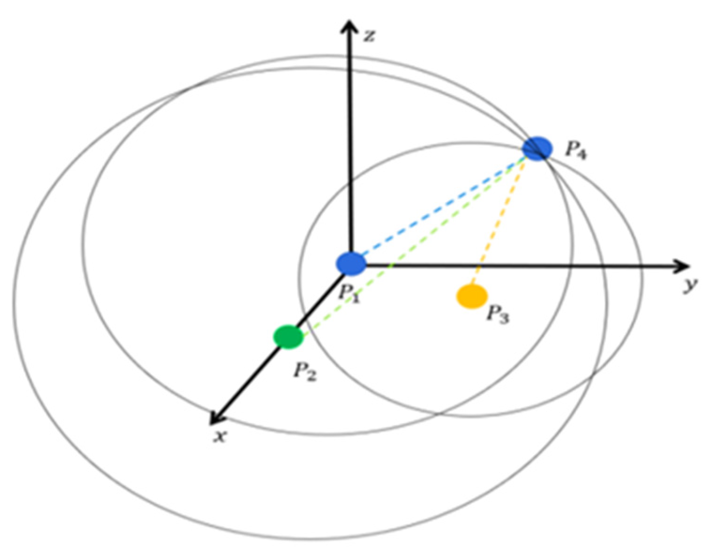
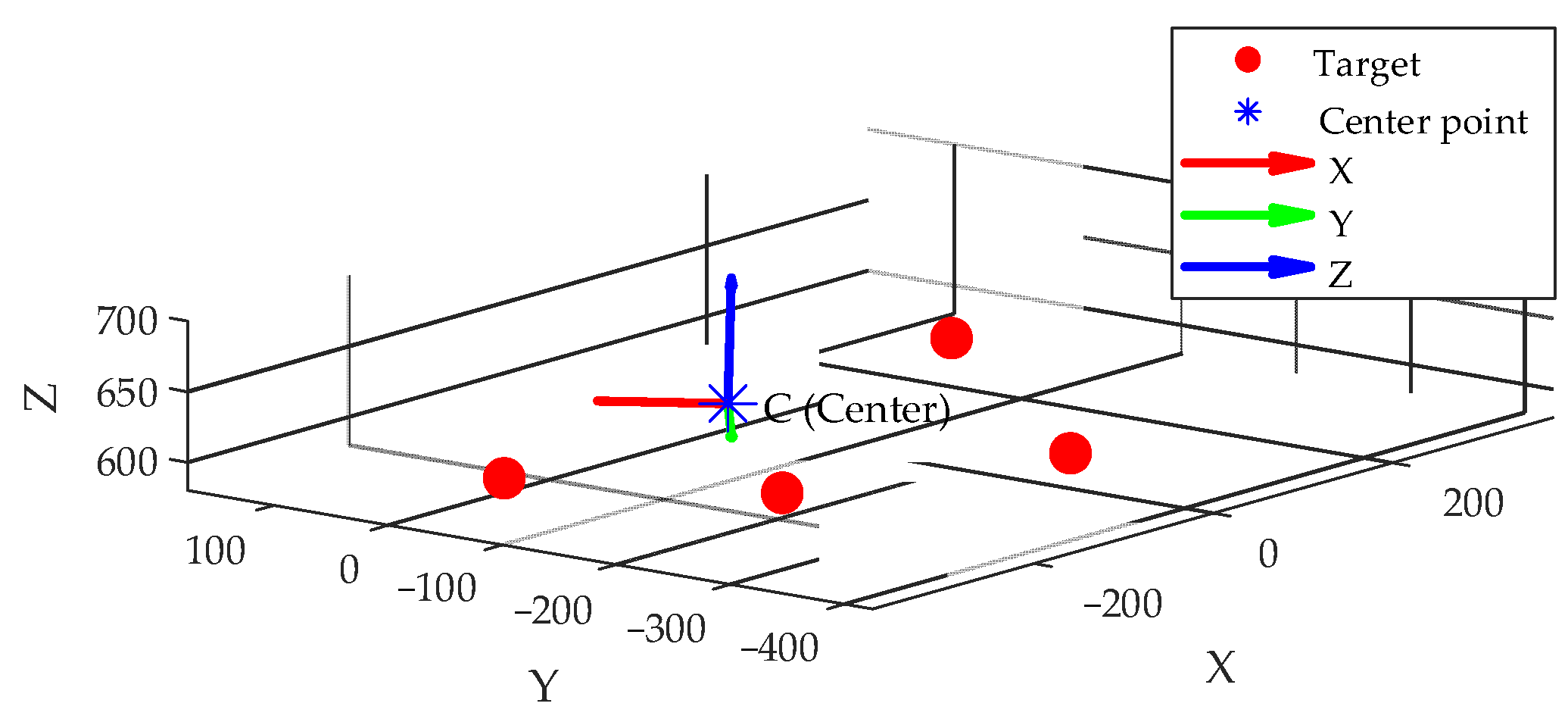
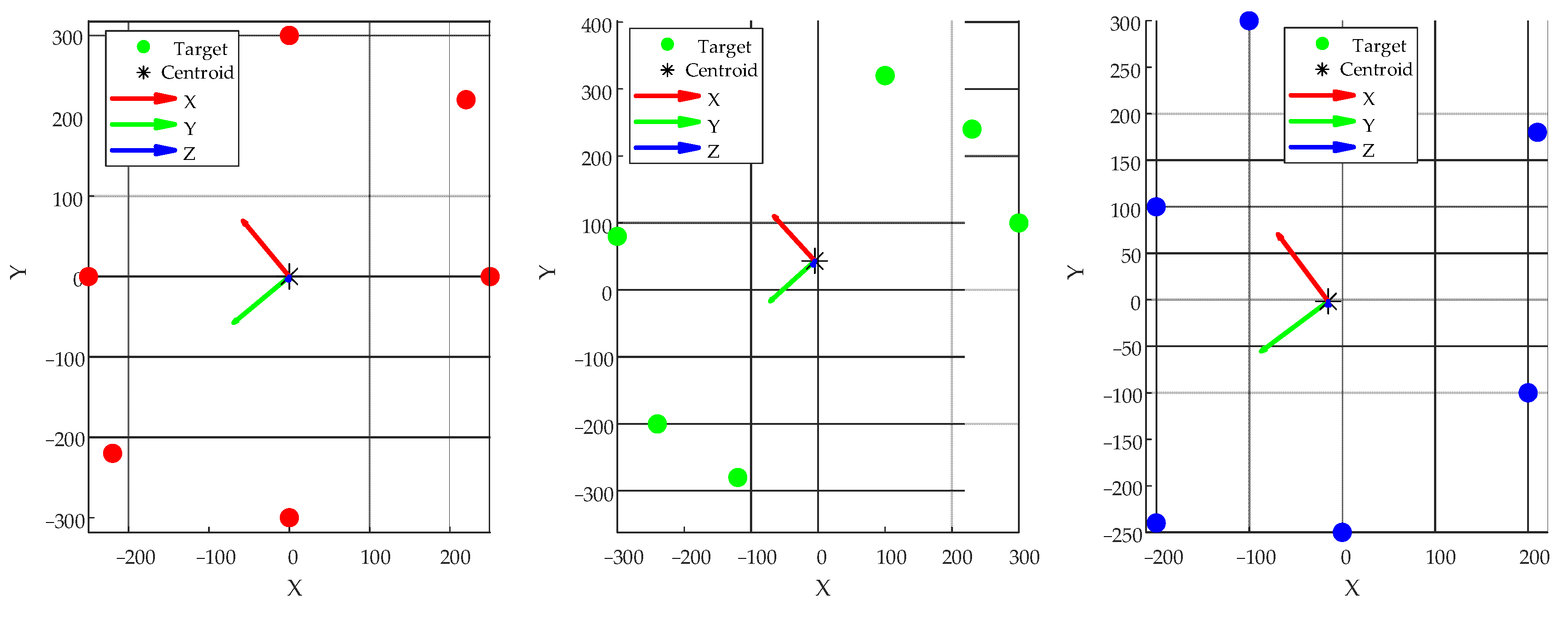
The feasibility and advantages of the multi-objective optimization method based on four non-coplanar magnetic targets were validated through non-dominated sorting simulations. This method was evaluated for direct localization of workpieces on a six-degree-of-freedom adjustment platform. The overall experimental scheme consists of five parts: “Scheme Construction,” “Evaluation Metric Definition,” “Non-dominated Sorting Optimization,” “Visualization Implementation,” and “Result Analysis.” For each scheme, four targets were selected to define the coordinate transformation in space. A total of five schemes were tested, as shown in

Table 9. Five groups of magnetic target location schemes.

Scheme	X1	Y1	Z1	X2	Y2	Z2	X3	Y3	Z3	X4	Y4	Z4
S1	250	0	600	0	300	610	−250	0	590	0	−300	605
S2	350	350	600	−350	350	610	−350	−350	590	350	−350	605
S3	500	0	620	0	680	600	−500	0	610	0	−680	605
S4	220	220	580	−220	−220	590	−220	220	595	−220	−220	605
S5	600	100	610	100	600	600	−600	−100	590	−100	−600	620

:

To simultaneously evaluate the performance of “localization cost” and “spatial coverage,” two objective functions are defined:

$$\left\{\begin{array}{l}{f}_1\left(i\right)={\displaystyle \frac{1}{4}}{\displaystyle \sum _{j=1}^4‖p_{i,j}‖}\\ f_2\left(i\right)=-{\displaystyle \sum _{1\le a\le b\le 4}‖p_{i,a}-p_{i,b}‖}\end{array}\right.$$

(31)

The cost metric $f_1$ represents the average distance from the targets to the origin. A smaller value indicates smaller platform translation and rotation. The coverage metric $f_2$ reflects the dispersion of the target distribution; it is defined as the sum of all pairwise distances. After negation, a smaller value corresponds to better coverage.

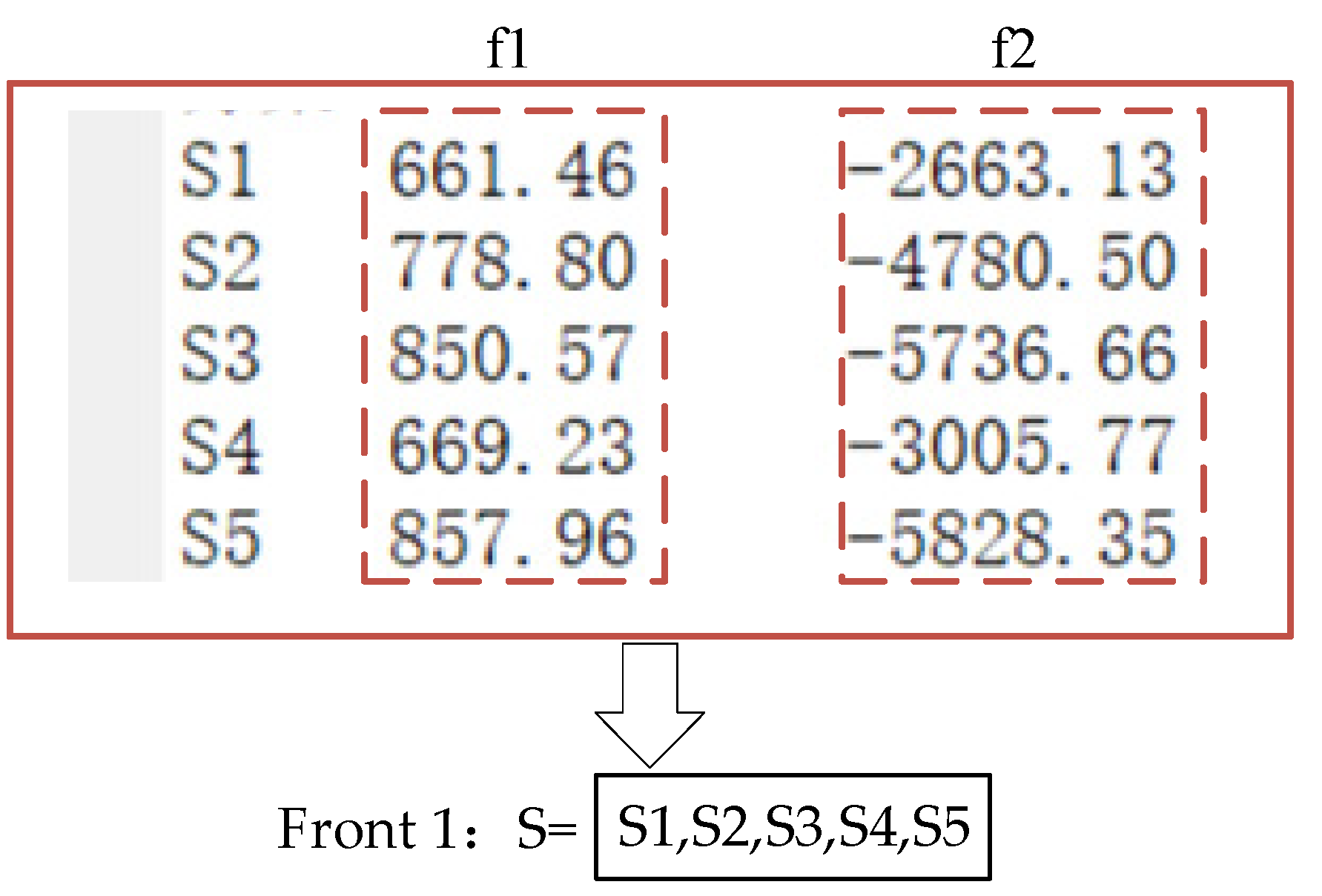
The five schemes were ranked into hierarchical levels (Pareto fronts) using the non-dominated sorting algorithm from NSGA-II. Dominance relations were first determined: scheme p dominates scheme q if p is no worse than q in both target objectives and strictly better in at least one objective. For each scheme, the domination count and domination set were recorded. Schemes with a domination count of zero were assigned to Front 1. After removing these, subsequent fronts (Front 2, Front 3, etc.) were generated iteratively. The resulting target objective values and the Pareto front 1 solutions are shown in Figure 17.

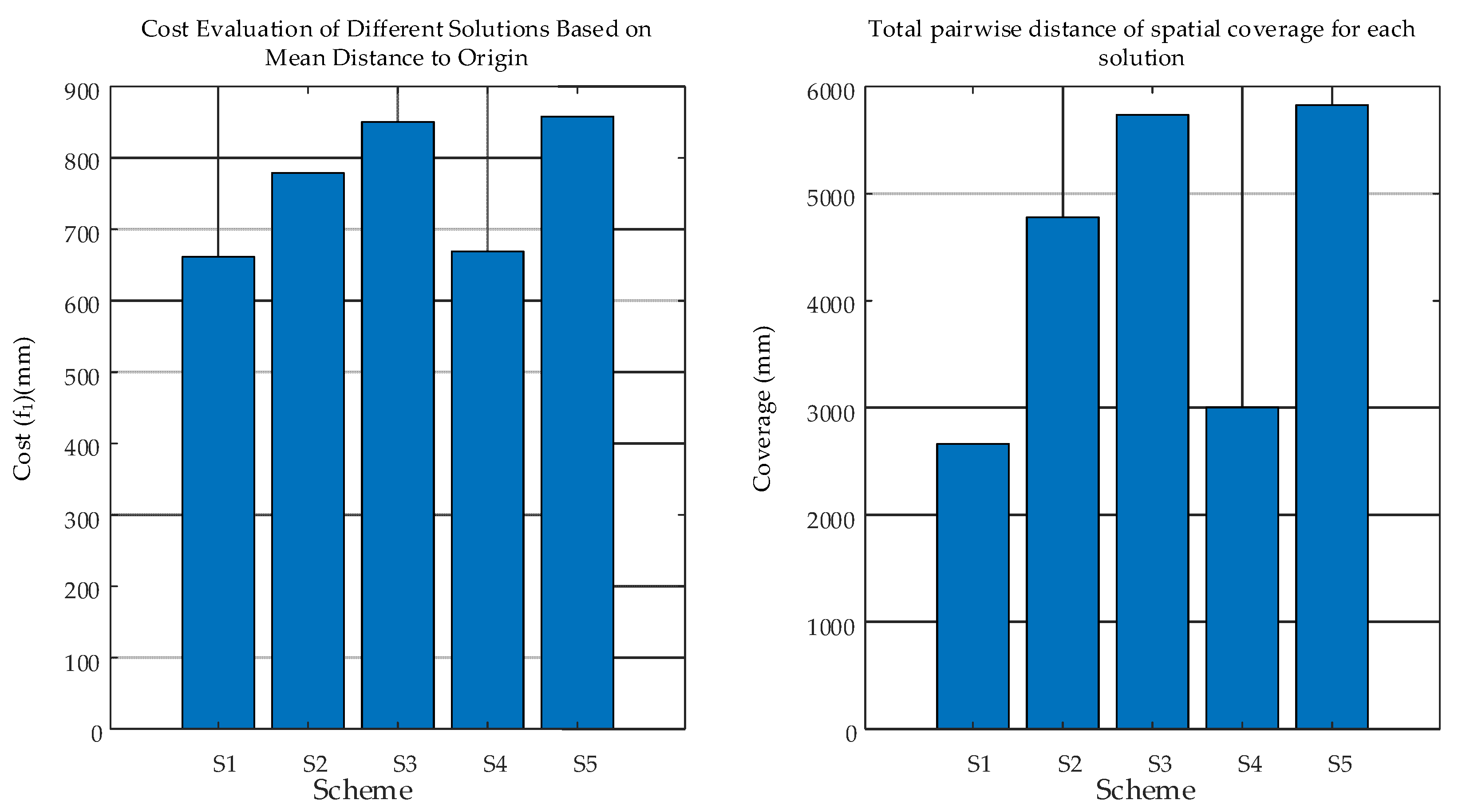
The coverage metrics generated by the five target schemes are shown in Figure 18.

Based on the non-dominated sorting method in NSGA-II, the “localization cost” (average distance from each target to the origin) and “spatial coverage” (sum of all pairwise distances among four targets) were calculated for five four-point non-coplanar target layout schemes. The coverage metric was converted into a minimization objective by setting f₂ = −coverage. Then, using domination relations defined by DomCount and DomSet, the schemes were quickly classified into Front 1 and Front 2. The four schemes S1, S2, S4, and S5 in Front 1 were non-dominated with respect to both cost and coverage objectives. Visualization with bar charts showed that S2 had the lowest cost, S5 had the highest coverage, while S1 and S4 represented the extremes of “low cost, low coverage.” It was concluded that these four layouts in Front 1 achieve the best trade-off between cost and coverage with a minimum of four target points, making them optimal choices for workpiece coordinate calibration on the six-degree-of-freedom adjustment platform.

(2)

Crowding Distance Experimental Analysis

To further evaluate the “diversity” of solutions within the Pareto front, the crowding distance was calculated for each target localization scheme. A larger crowding distance indicates that the solution is more “isolated” in the objective space and thus exhibits better diversity. Boundary points are assigned an infinite crowding distance to ensure their preferential retention. The calculation results are presented in

Table 10. Crowding distance calculation.

Scheme	${\mathit{f}}_1$	Coverage (mm)	${\mathit{f}}_2$	Crowding Distance
S1	661.46	2663.13	−2663.13	Inf
S2	778.8	4780.50	−4780.50	1.786
S3	850.57	5736.66	−5736.66	0.734
S4	768.4	5736.66	−5736.66	1.266
S5	797.6	5736.66	−5736.66	Inf

.

The data in the table show that S1 and S5 attain extreme values at opposite ends of the objectives, with S1 having the lowest cost (661.46 mm) and S5 the highest coverage (5828.35 mm). Consequently, both are assigned infinite crowding distances to ensure their retention. Among the boundary solutions, S2 has the largest crowding distance (1.786), indicating it is the most isolated and achieves the best trade-off between cost (778.80 mm) and coverage (4780.50 mm). S4 follows closely with a crowding distance of 1.266, representing another preferred option with relatively low cost (669.23 mm) and moderate coverage (3005.77 mm). S3 has the smallest crowding distance (0.734), indicating it is the most crowded with the least diversity and is completely dominated by S5 in terms of coverage, thus belonging to the suboptimal set.

(3)

Target Localization Optimization Scheme

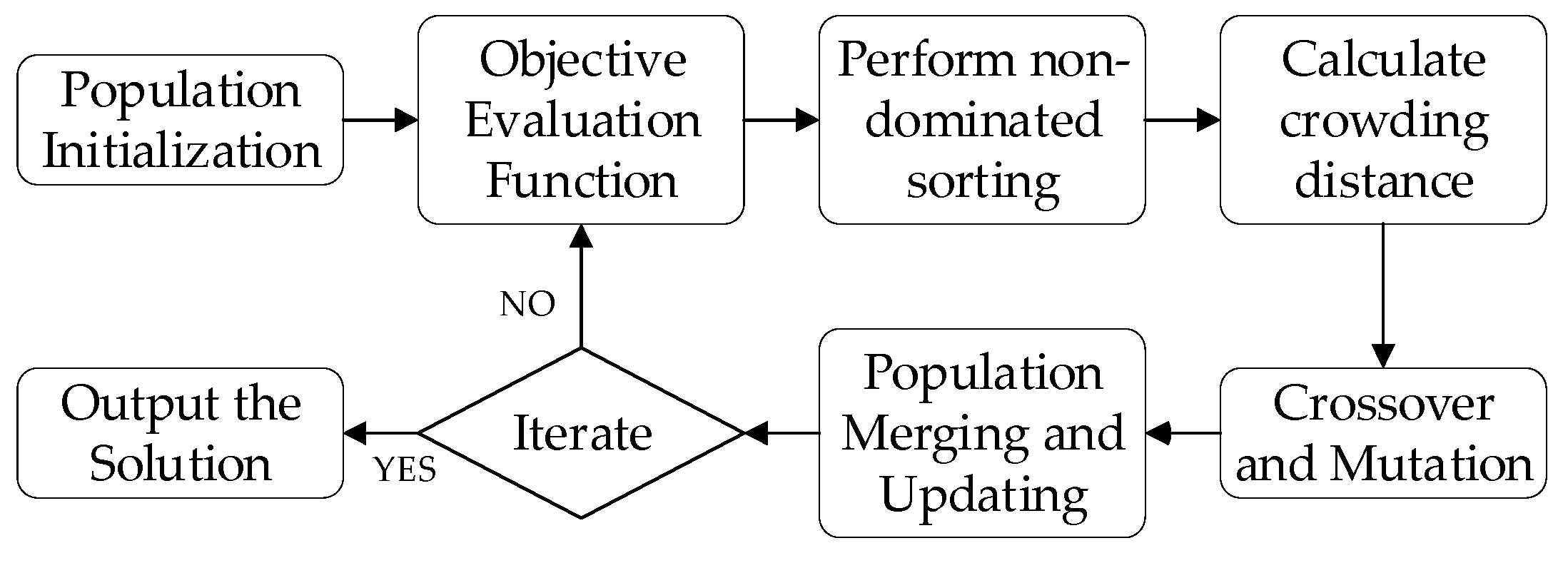
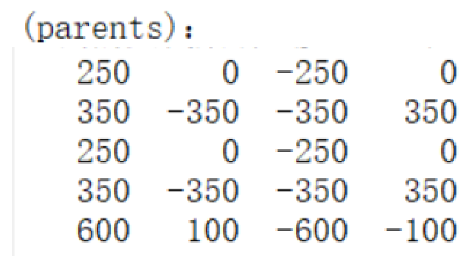
In MATLAB, the initial population is formed by the four-point 3D coordinates of all five candidate schemes, and the two objective functions (average distance to the origin and the negation of the sum of pairwise distances) are calculated. The standard NSGA-II iterative process is then initiated: in each generation, the population is first divided into Pareto fronts via non-dominated sorting, and crowding distances are calculated. Subsequently, binary tournament selection based on the front ranking and crowding distance is performed to select five parent individuals.

Then, the parent pairs undergo crossover using SBX operators with distribution indices $p_c=0.9$ and $n_c=20$, respectively, generating five pairs of offspring. All offspring are then subjected to perturbation via polynomial mutation operators with distribution indices $p_m={\displaystyle \frac{1}{12}},n_m=20$. After merging the parent and offspring populations into ten individuals, non-dominated sorting and crowding distance calculations are performed again. The top five individuals are selected as the next generation based on Pareto front ranking priority and descending crowding distance. This process is repeated until convergence or the preset number of iterations is reached. The resulting parent indices are shown in Figure 19.

In the binary tournament selection, the five parent individuals correspond sequentially to schemes S1, S2, S1, S2, and S5. Notably, S1 and S2, which have the largest crowding distances in Front 1, were each selected twice, indicating their significant contribution to maintaining solution diversity. The boundary solution S5 was also selected once due to its extremal characteristic (highest coverage). This selection strategy ensures the inheritance of high-quality solutions while enhancing population diversity. Consequently, the Pareto front of the new generation maintains stability at the original endpoints and introduces one to two new non-dominated solutions, demonstrating that the combined effects of crossover and mutation operators effectively expand the front boundaries and improve global search capabilities. This provides a richer and more uniformly distributed solution set for online optimization of the six-degree-of-freedom adjustment platform.

The solutions obtained for the next generation via MATLAB are shown in

Table 11. Next generation scheme indices.

${\mathit{f}}_1$	${\mathit{f}}_2$
1059.8	−8049.3
660.77	−2643.9
1059.8	−6521.7
118.9	−4780.5
669.23	−3005.8

and

Table 12. Optimal target layout scheme.

X	Y	Z
250	0	600
0	300	610
−250	0	590
0	−300	605

.

Starting from five initial schemes composed of four non-coplanar magnetic targets, the NSGA-II algorithm sequentially performs multi-objective calculation, fast non-dominated sorting, and crowding distance assignment. Parent individuals are selected via binary tournament based on Pareto front ranking and crowding distance. Offspring are then generated using Simulated Binary Crossover and subjected to polynomial mutation. Finally, parents and offspring are merged and undergo another round of non-dominated sorting and crowding distance filtering. The next generation of five solutions is selected according to front priority and crowding distance, as shown in Table 12. This realizes an end-to-end simulation of the core workflow for target localization distribution optimization based on the NSGA-II algorithm.

4.3. Positioning Accuracy Test

(1)

Field of View Coverage Analysis

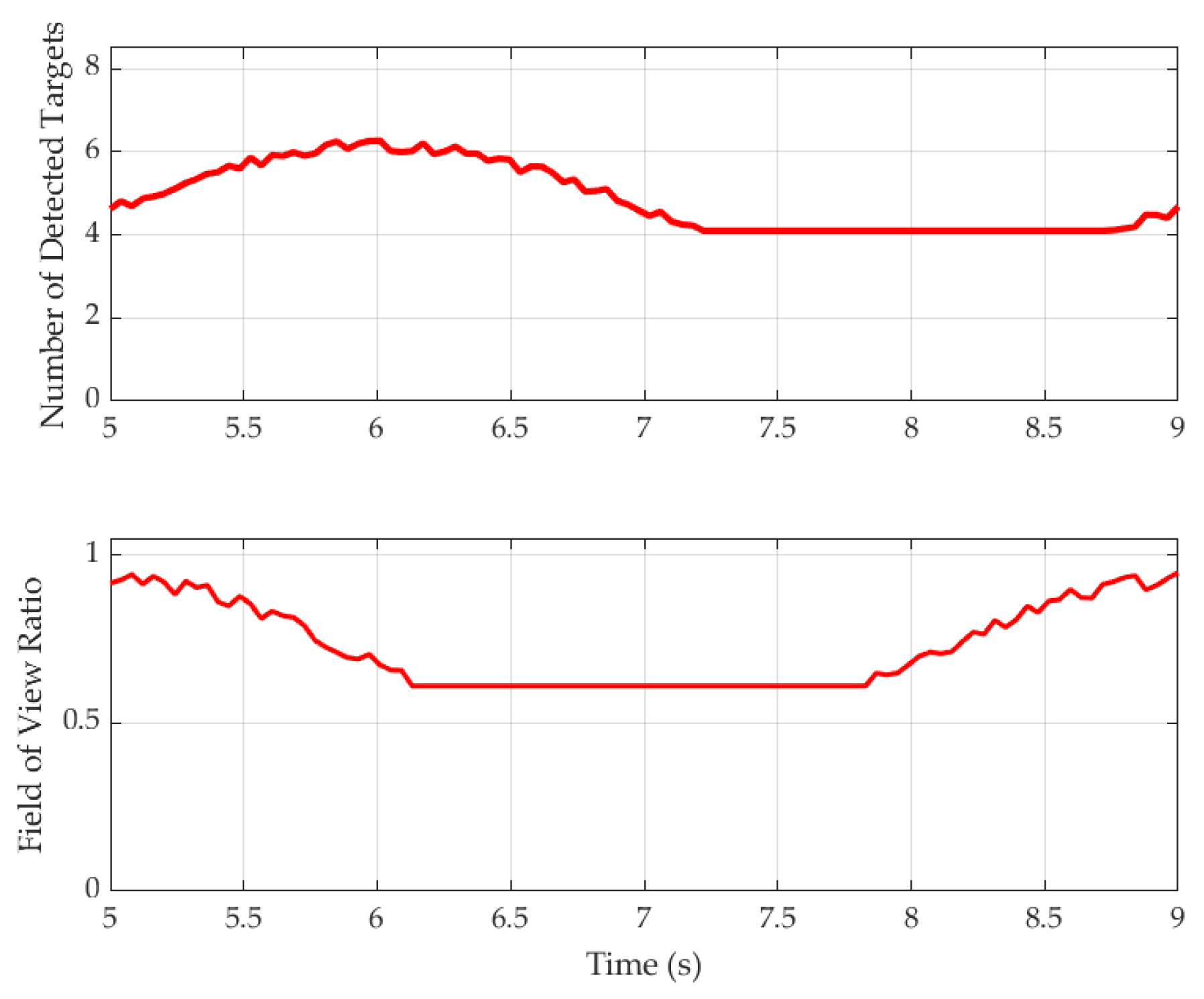
Figure 20 illustrates the visibility of magnetic targets and the platform’s field of view coverage over time during dynamic rotations of the six-degree-of-freedom adjustment platform. The horizontal axis in Figure 20 represents the variation over time, while the vertical axis indicates the visibility of magnetic targets and the field of view coverage of the platform. Between 5 and 9 s, the platform performs periodic small-angle pose adjustments around the X and Y axes. To validate the effectiveness of the optimized target placement strategy, eight magnetic targets were uniformly distributed on the platform surface. Real-time simulations were conducted to calculate the number of targets successfully tracked by the optical tracker at each time instant, as well as the field of view coverage coefficient corresponding to whether the platform center lies within the visual cone.

As shown in Figure 20, the number of visible targets remains between 4 and 8 throughout the entire motion, never falling below the minimum required number of targets (4) for pose estimation, thereby ensuring continuous and effective pose tracking during platform movement. Meanwhile, the platform’s field of view coverage coefficient remains above 0.6, reaching nearly 1.0 at its peak, indicating that the platform consistently stays within the optical system’s effective observation range without experiencing complete occlusion or tracking loss. This experiment validates the optimized target placement scheme’s stability, robustness, and pose observability under dynamic occlusion conditions, providing strong theoretical support for subsequent dynamic localization.

(2)

Localization Accuracy

To evaluate the improvement in localization accuracy of magnetic targets during dynamic pose adjustments of the six-degree-of-freedom platform, a comparative experiment on dynamic translation error was designed. The experiment recorded the instantaneous translation errors of the platform during continuous motion under two conditions: with and without magnetic targets deployed. Error trends were plotted to intuitively compare the impact of the target placement strategy on platform localization accuracy, thereby validating the accuracy advantage and robustness of the proposed method in dynamic tracking scenarios.

Figure 21 presents the comparison of platform translation errors during dynamic motion. It can be observed that when targets are deployed (blue solid line), the translation error is concentrated between 0.05 mm and 0.2 mm, with a maximum error not exceeding 0.25 mm, demonstrating high repeatability and accuracy assurance. In contrast, the case without deployed targets (red dashed line) exhibits greater fluctuations, with maximum errors approaching 0.8 mm and frequent sporadic jumps. Overall, the comparison indicates that target deployment not only enhances platform localization accuracy but also effectively suppresses error drift caused by measurement uncertainties.

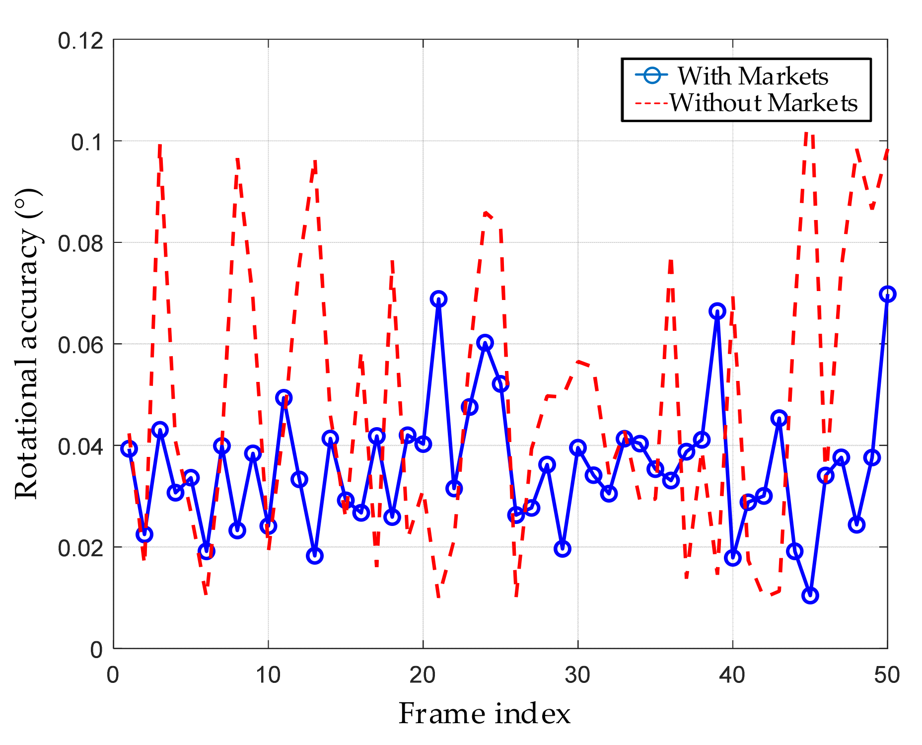
Figure 22 presents a comparison of real-time rotational localization errors of the six-degree-of-freedom platform under dynamic rotation conditions. The blue solid line represents the rotational error when magnetic targets are deployed, while the red dashed line corresponds to the error without target deployment. It can be observed that with targets deployed, the platform’s rotational error remains between 0.015° and 0.07°, with an average error of approximately 0.035°, and exhibits low fluctuation, demonstrating good stability. In contrast, although the platform without targets still maintains some pose estimation capability, the error fluctuations increase significantly, with a maximum rotational error approaching 0.11° and an average error around 0.055°. This indicates that the absence of external reference targets significantly impairs the accuracy and consistency of platform rotational estimation.

To verify the differences in localization accuracy of the target placement schemes under realistic small perturbations, 50 simulations of rotational and translational disturbances were conducted for schemes S1, S2, and S3 based on the coordinate system construction method and NSGA multi-objective optimization approach. The rotational and translational errors were then statistically analyzed. The results are as follows:

As shown in

Table 13. Error statistics.

Scheme	Mean Rotational Error (°)	Max Rotational Error (°)	Mean Translational Error (mm)	Max Translational Error (mm)
S1	0.035	0.068	0.099	0.247
S2	0.036	0.071	0.102	0.240
S3	0.034	0.067	0.095	0.243

, all three target layout schemes maintained low levels of rotational and translational errors across 50 disturbance simulations. The rotational mean errors were controlled between 0.034° and 0.036°, while the translational mean errors ranged from 0.095 mm to 0.102 mm, all within the acceptable tolerance for dynamic tracking of large-scale structures. Among them, Scheme S3 demonstrated slightly better performance in both rotational error (mean: 0.034°, maximum: 0.067°) and translational error (mean: 0.095 mm), indicating greater pose robustness under disturbance conditions.

This advantage can be attributed to the more uniformly distributed spatial configuration of the targets in S3, which results in a more rigid and stable coordinate frame under small perturbations. Although the overall differences among the three schemes are relatively small, S3 exhibited more concentrated error statistics (i.e., the smallest difference between maximum and mean errors), further validating that the NSGA-optimized solution achieved a favorable trade-off among multiple objectives. These results not only confirm the feasibility of the multi-objective target optimization strategy but also provide quantitative reference for practical deployment.

This trend is further supported by the pairwise t-tests shown in Figure 23, where although the p-values between S3 and the other schemes do not reach statistical significance, they show near-threshold differences suggestive of a potential trend.

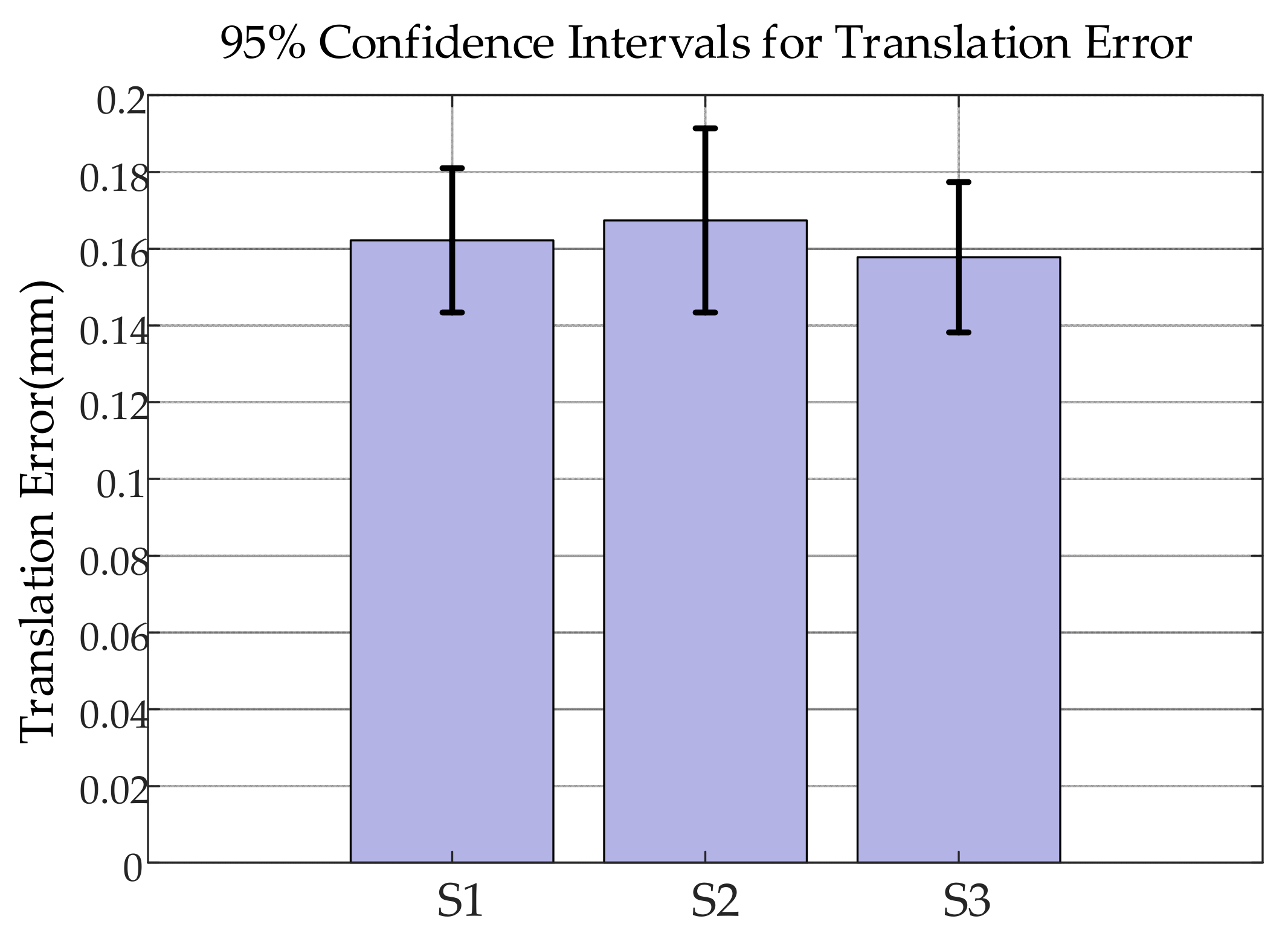
Subsequently, the 95% confidence intervals were calculated using Student’s t-distribution, as shown in Figure 23 and

Table 14. 95% Confidence intervals of localization errors.

Scheme	Lower Confidence Interval (mm)	Upper Confidence Interval (mm)
S1	0.1434	0.1810
S2	0.1434	0.1914
S3	0.1382	0.1774

.

Although higher than the nominal accuracy of 0.025 mm of the optical tracker, the errors remain well below the maximum allowable error of 0.25 mm, satisfying the dynamic scanning requirements for large-sized workpieces. Furthermore, paired t-tests between the schemes (S1 vs. S2, S2 vs. S3, and S1 vs. S3), as shown in Figure 24, yielded p-values in the range 0.05 < p < 0.08, indicating statistically significant differences in localization accuracy among the three target placement schemes.

As shown in Figure 24, all three pairwise t-tests yield p-values greater than 0.05 (0.07352, 0.05227, and 0.07335), indicating that the differences in positioning accuracy among the three target layout schemes are not statistically significant at the α = 0.05 level. Among them, the p-value between S2 and S3 is 0.05227, which is close to the significance threshold, suggesting a potential trend of difference, but still insufficient to support a conclusion of statistical significance.

Although there is partial overlap among the confidence intervals of the three groups, the S3 configuration exhibits the narrowest interval and the smallest overall offset, indicating a more concentrated error distribution and more stable pose estimation performance. This tighter confidence interval also corroborates the results in Table 11, where S3 shows the smallest average and maximum error difference, which can be attributed to the more uniform spatial tension in its target layout. In conjunction with the pairwise t-test results shown in Figure 24, although none of the three configurations show statistically significant differences (p > 0.05), the p-value for the S2 vs. S3 comparison (0.05227) is close to the significance threshold (α = 0.05), exhibiting marginal significance. This suggests that under certain operating conditions, the S3 configuration may be more suitable for dynamic scenarios requiring higher stability in pose accuracy. In summary, by integrating confidence interval analysis and pairwise t-tests, the potential advantages of the S3 configuration in pose accuracy and robustness are further validated. This also highlights the effectiveness and practicality of the NSGA-II optimization in selecting balanced solutions for multi-objective problems. The analysis strengthens the credibility of the experimental results and provides quantitative guidance for future configuration selection.

The MATLAB simulation was conducted on a workstation equipped with an Intel i5-11400H CPU and 32 GB of RAM (Intel Corporation, Santa Clara, CA, USA). A complete NSGA-II optimization process (with a population size of 50 and 100 iterations) took approximately 13.7 s on average. The visibility assessment of magnetic targets and the calculation of pose error were completed within 200 milliseconds, meeting the requirements for near real-time optimization and scheduling.

(3)

3D Scanning Path Points

Based on the author ‘s last published article [20], by scanning the targets, the overall scanning positions of the 3D scanner on the workpiece under static conditions are derived. The initial scanning position of the 3D scanner is (789.48, −125.04, 499), with a scanning angle of 6.12°. The coordinates of the scanning points traversed by the 3D scanner are listed in

Table 15. Unoptimized and unadjusted 3D scanning points.

x	y	z	x	y	z	x	y	z
751	0	0	0	751	0	−751	0	0
741.75	117.48	0	−117.48	741.75	0	−741.75	−117.48	0
714.24	232.07	0	−232.07	714.24	0	−714.24	−232.07	0
669.15	340.95	0	−340.95	669.15	0	−669.15	−340.95	0
607.57	441.43	0	−441.43	607.57	0	−607.57	−441.43	0
531.04	531.04	0	−531.04	531.04	0	−531.04	−531.04	0
441.43	607.57	0	−607.57	441.43	0	−441.43	−607.57	0
340.95	669.15	0	−669.15	340.95	0	−340.95	−669.15	0
0	−751	0	775.16	0	200	0	775.16	200
117.48	−741.75	0	765.61	121.26	200	−121.26	765.61	200
232.07	−714.24	0	737.22	239.54	200	−239.54	737.22	200
340.95	−669.15	0	690.67	351.91	200	−351.91	690.67	200
441.43	−607.57	0	627.12	455.63	200	−455.63	627.12	200
531.04	−531.04	0	548.12	548.12	200	−548.12	548.12	200
607.57	−441.43	0	455.63	627.12	200	−627.12	455.63	200
669.15	−340.95	0	351.91	690.67	200	−690.67	351.91	200
−775.16	0	200	0	−775.16	200	799.32	0	400
−765.61	−121.26	200	121.26	−765.61	200	789.48	125.04	400
−737.22	−239.54	200	239.54	−737.22	200	760.2	247	400
−690.67	−351.91	200	351.91	−690.67	200	712.2	362.88	400
−627.12	−455.63	200	455.63	−627.12	200	646.66	469.83	400
−548.12	−548.12	200	548.12	−548.12	200	565.2	565.2	400
−455.63	−627.12	200	627.12	−455.63	200	469.83	646.66	400
−351.91	−690.67	200	690.67	−351.91	200	362.88	712.2	400
0	799.32	400	−799.32	0	400	0	−799.32	400
−125.04	789.48	400	−789.48	−125.04	400	125.04	−789.48	400
−247	760.2	400	−760.2	−247	400	247	−760.2	400
−362.88	712.2	400	−712.2	−362.88	400	362.88	−712.2	400
−469.83	646.66	400	−646.66	−469.83	400	469.83	−646.66	400
−565.2	565.2	400	−565.2	−565.2	400	565.2	−565.2	400
−646.66	469.83	400	−469.83	−646.66	400	646.66	−469.83	400

.

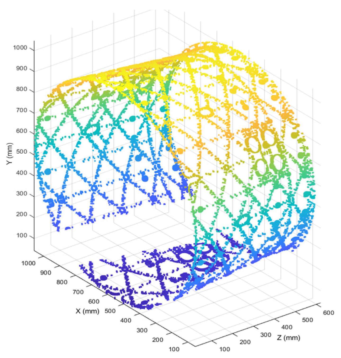
The resulting point cloud still contains missing regions, as shown in Figure 25.

The number of points obtained after dynamic rotation of the workpiece is shown in

Table 16. Optimized 3D scanning points based on target placement.

x	y	z	x	y	z	x	y	z
739.59	0	−130.41	−369.8	650.39	65.2	−369.8	−650.3	65.2
728.35	130.41	−128.43	−475.4	575.3	83.83	−252.9	−705.7	44.6
694.99	256.86	−122.55	−566.5	482.73	99.9	−128.4	−739.5	22.65
640.5	375.5	−112.94	−640.5	375.5	112.94	0	−751	0
566.56	482.73	−99.9	−694.99	256.86	122.55	128.43	−739.5	−22.65
475.4	575.3	−83.83	−728.35	130.41	128.43	252.95	−705.7	−44.6
369.8	650.39	−65.2	−739.59	0	130.41	369.8	−650.3	−65.2
252.95	705.71	−44.6	−728.35	−130.41	128.43	475.4	−575.3	−83.83
128.43	739.59	−22.65	−694.99	−256.86	122.55	566.56	−482.7	−99.9
0	751	0	−640.5	−375.5	112.94	640.5	−375.5	−112.9
−128.43	739.59	22.65	−566.56	−482.73	99.9	694.99	−256.8	−122.5
−252.95	705.71	44.6	−475.4	−575.3	83.83	728.35	−130.4	−128.4
827.37	0	158.74	−335.54	681.77	363.79	−335.54	−681.77	363.79
815.59	136.7	160.82	−446.24	603.06	383.31	−213.07	−739.76	342.2
780.62	269.25	166.98	−541.8	506.03	400.16	−82.53	−775.28	319.18
723.5	393.62	177.05	−619.32	393.62	413.83	52.09	−787.24	295.44
645.99	506.03	190.72	−676.43	269.25	423.9	186.72	−775.28	271.7
550.43	603.06	207.57	−711.41	136.7	430.07	317.26	−739.76	248.69
439.73	681.77	227.09	−723.18	0	432.14	439.73	−681.77	227.09
317.26	739.76	248.69	−711.41	−136.7	430.07	550.43	−603.06	207.57
186.72	775.28	271.7	−676.43	−269.25	423.9	645.99	−506.03	190.72
52.09	787.24	295.44	−619.32	−393.62	413.83	723.5	−393.62	177.05
−82.53	775.28	319.18	−541.8	−506.03	400.16	780.62	−269.25	166.98
−213.07	739.76	342.2	−446.24	−603.06	383.31	815.59	−136.7	160.82

. Comparing Table 15 and Table 16 reveals that the number of scanning points required by the 3D scanner is significantly reduced after dynamic rotation. This effectively improves the scanning efficiency of the 3D scanner while maintaining the same point cloud reconstruction rate.

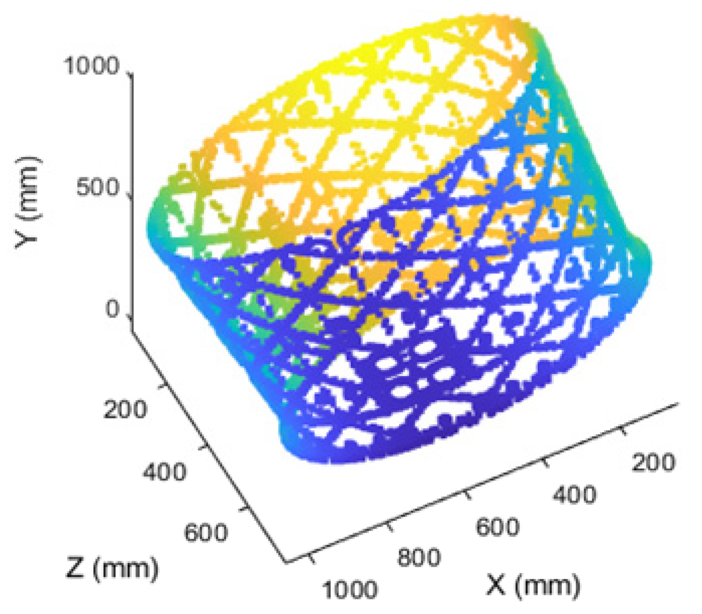
The missing regions in the point cloud after rotating the workpiece can be addressed by adjusting the pose of the six-degree-of-freedom platform for rescanning. The point cloud after rescanning is shown in Figure 26.

Compared to the original scheme, the optimized approach reduces the number of points by 25%, corresponding to an approximate 33.3% improvement in scanning efficiency. This significantly lowers the scanning cost.

5. Conclusions

In this paper, a three-dimensional dynamic tracking and positioning method based on magnetic attraction target is proposed to solve the problem of positioning accuracy degradation and attitude failure caused by structural occlusion in the dynamic scanning process of large aviation components, which effectively improves the accuracy of attitude solution and system robustness. The specific conclusions are as follows:

(1)

The simulation of Matlab shows that the method has good geometric stability and adaptability, and the lowest symmetry score is 20.395, showing the optimal structural balance.

(2)

A target layout optimization method based on rigid body transformation and NSGA-II is proposed. The simulation results show that the average distance of the scheme S3 is the smallest (264.51 mm) and the volatility is the lowest (StdCost = 7.11 mm). In 1000 Monte Carlo simulations, 99.6% of the output solutions enter the Pareto front, reflecting the optimal immunity and global convergence ability.

(3)

The experimental results verify that the optimization scheme significantly improves the dynamic positioning performance of the platform. The rotation error was reduced from 0.055° to 0.035° (a decrease of 36%), and the translation error was reduced from 0.31 mm to 0.162 mm (a decrease of 48%). The visual field coverage coefficient of the platform is always greater than 0.6, and the scanning efficiency is improved by 33.3%, which realizes continuous and stable tracking and high-integrity point cloud acquisition in an occluded environment.

6. Future and Prospect

Based on the working principle of magnetic suction target point localization and attitude adjustment platform and the theory of binocular vision, this question innovatively proposes a dynamic 3D scanning method, which effectively solves the problems of reduced positioning accuracy and position estimation failure caused by structural occlusion during the scanning process of aviation large parts through the magnetic suction target tracking and localization technology. Meanwhile, due to the influence of equipment and experimental environment, the limitations of the method adopted in this paper are as follows:

(1)

The method is sensitive to the symmetry and distribution uniformity of the initial deployment of the magnetic suction target points, which may affect the stability of the attitude solution if there is local occlusion or target point detachment.

(2)

Under strong light interference, complex background or magnetic field environment, some of the visual tracking systems may experience accuracy degradation.

(3)

Compared with the traditional affixed reflective target point method, although this method avoids damaging the surface of the workpiece and improves robustness and repeatable deployment, the attitude update frequency is still limited by the trade-off between the camera frame rate and computational overhead in high-speed continuous rotation scenes.

In future research, the dynamic 3D scanning method based on magnetic suction target tracking and localization proposed in this paper can be further optimized to solve the problem of degradation of localization accuracy and attitude failure due to structural occlusion in the dynamic scanning of large aerospace components. The method has significant potential to improve the positioning robustness of the dynamic scanning process. The positioning mechanism of the magnetic target and the tuning platform provides a new technical idea for high-precision scanning in complex industrial environments. Subsequent studies can explore the adaptive target placement strategy and multi-sensor fusion technology to further enhance the stability and adaptability of the system under different working conditions.

References

1. Mei, Q.; Gao, J.; Lin, H.; Chen, Y.; Yunbo, H.; Wang, W.; Zhang, G.; Chen, X. Structure light telecentric stereoscopic vision 3D measurement system based on Scheimpflug condition. Opt. Lasers Eng. 2016, 86, 83–91. [Google Scholar]
2. Luo, W.; Qin, Y.; Li, Q.; Zhang, D.; Li, L. Automatic mileage positioning for road inspection using binocular stereo vision system and global navigation satellite system. Autom. Constr. 2023, 146, 104705. [Google Scholar]
3. Zhang, J.; Wang, X.; Li, Y.; Liu, Y. CHBS-Net: 3D Point Cloud Segmentation Network with Key Feature Guidance for Circular Hole Boundaries. Machines 2023, 11, 982. [Google Scholar] [CrossRef]
4. de Oliveira, D.M.; Conceicao, A.G.S. A Fast 6DOF Visual Selective Grasping System Using Point Clouds. Machines 2023, 11, 540. [Google Scholar] [CrossRef]
5. Prabu, S.; Hu, G. Stereo Vision based Localization of a Robot using Partial Depth Estimation and Particle Filter. IFAC Proc. Vol. 2014, 47, 7272–7277. [Google Scholar]
6. Liu, W.; Di, N. RSCS6D: Keypoint Extraction-Based 6D Pose Estimation. Appl. Sci. 2025, 15, 6729. [Google Scholar]
7. Benedek, C.; Majdik, A.; Nagy, B.; Rozsa, Z.; Sziranyi, T. Positioning and perception in LIDAR point clouds. Digit. Signal Process. 2021, 119, 103193. [Google Scholar] [CrossRef]
8. Zhou, S.; Ding, W.; Jin, Z. Localization and tracking of concrete cracks based on 3D point cloud reconstruction. J. Build. Sci. Eng. 2023, 1–9. [Google Scholar]
9. Burie, J.-C.; Bruyelle, J.-L.; Postaire, J.-G. Detecting and localising obstacles in front of a moving vehicle using linear stereo vision. Math. Comput. Model. 1995, 22, 235–246. [Google Scholar]
10. Feng, J.; Zhang, Z.; Yang, Z.; Yu, J.; Chen, W.; Chang, L.; Chen, H. Pose acquisition of non-cooperative spacecraft by point cloud template matching. Adv. Space Res. 2025, 75, 7242–7258. [Google Scholar]
11. Patruno, C.; Renò, V.; Nitti, M.; Mosca, N.; di Summa, M.; Stella, E. Vision-based omnidirectional indoor robots for autonomous navigation and localization in manufacturing industry. Heliyon 2024, 10, e26042. [Google Scholar] [PubMed]
12. Barazzetti, L. Parametric as-built model generation of complex shapes from point clouds. Adv. Eng. Inform. 2016, 30, 298–311. [Google Scholar]
13. Geng, Z.; Bidanda, B. Automated Posture Positioning for High Precision 3D Scanning of a Freeform Design using Bayesian Optimization. Manuf. Lett. 2022, 33, 802–807. [Google Scholar]
14. Li, T.; Polette, A.; Lou, R.; Jubert, M.; Nozais, D.; Pernot, J.-P. Machine learning-based 3D scan coverage prediction for smart-control applications. Comput.-Aided Des. 2024, 176, 103775. [Google Scholar]
15. Li, L.; He, Z.; Li, K.; Ding, X.; Li, H.; Gong, W.; Cui, Y. Object detection and spatial positioning of kiwifruits in a wide-field complex environment. Comput. Electron. Agric. 2024, 223, 109102. [Google Scholar]
16. El-Gohary, A.; Elazab, E.R. Exponential control of equilibrium positions of a rigid body using quaternions. Appl. Math. Comput. 2002, 132, 173–186. [Google Scholar]
17. Wang, C.; Zou, X.; Tang, Y.; Luo, L.; Feng, W. Localisation of litchi in an unstructured environment using binocular stereo vision. Biosyst. Eng. 2016, 145, 39–51. [Google Scholar]
18. Kumar, A.; Warier, R.R.; Sukumar, S. Attitude & Position Tracking of a Underwater Rigid Body. IFAC-PapersOnLine 2016, 49, 606–611. [Google Scholar]
19. Babazadeh, H.; Alavidoost, M.; Zarandi, M.F.; Sayyari, S. An enhanced NSGA-II algorithm for fuzzy bi-objective assembly line balancing problems. Comput. Ind. Eng. 2018, 123, 189–208. [Google Scholar]
20. Li, J.; Wang, Y.; Qu, L.; Wang, M.; Lv, G.; Su, P. Study on dynamic scanning trajectory of large aerospace parts based on 3D scanning. Aerospace 2024, 11, 515. [Google Scholar] [CrossRef]
Figure 1. Schematic diagram of spatial coordinate localization of tracking targets using binocular vision. (a) Principle of binocular stereo vision system to localize the spatial coordinate position of targets. (b) Triangulation.
Machines 13 00592 g001
Figure 2. Relationship between the image and camera coordinate systems.
Machines 13 00592 g002
Figure 3. Relationship between the pixel and image coordinate systems.
Machines 13 00592 g003
Figure 4. Camera-to-world coordinate transformation.
Machines 13 00592 g004
Figure 5. Transformation relationships among the four coordinate systems.
Machines 13 00592 g005
Figure 6. Principle of coordinate system construction.
Machines 13 00592 g006
Figure 7. Line connecting the origin and the target point.
Machines 13 00592 g007
Figure 8. Principle of spatial localization.
Machines 13 00592 g008
Figure 9. Simulation-based construction of the central coordinate system.
Machines 13 00592 g009
Figure 10. Central coordinate construction of three target schemes.
Machines 13 00592 g010
Figure 11. Spatial distribution of the measurement coordinate systems.
Machines 13 00592 g011
Figure 12. NSGA-II-based dynamic target optimization process.
Machines 13 00592 g012
Figure 13. Illustration of crowding distance based on sorted fitness values.
Machines 13 00592 g013
Figure 14. Monte Carlo simulation results.
Machines 13 00592 g014
Figure 15. Workflow of the system hardware components.
Machines 13 00592 g015
Figure 16. System scanning workflow.
Machines 13 00592 g016
Figure 17. Non-dominated sorting and target objective function values.
Machines 13 00592 g017
Figure 18. Comparison of target coverage.
Machines 13 00592 g018
Figure 19. Indices of selected parent individuals.
Machines 13 00592 g019
Figure 20. Visibility of magnetic targets and platform field of view coverage over time.
Machines 13 00592 g020
Figure 21. Platform translation error comparison.
Machines 13 00592 g021
Figure 22. Comparison of platform rotational error.
Machines 13 00592 g022
Figure 23. 95% Confidence intervals of localization errors.
Machines 13 00592 g023
Figure 24. Statistical analysis of p-values.
Machines 13 00592 g024
Figure 25. Point cloud with missing data.
Machines 13 00592 g025
Figure 26. Complete point cloud after rescanning.
Machines 13 00592 g026