Parameter Stress Response Prediction for Vehicle Dust Extraction Fan Impeller Based on Feedback Neural Network

Abstract

Vehicles exhibit complex failure modes and mechanisms because of their extreme service environments and severe external loads. The increasing level of integration in these vehicles is also driving more stringent reliability requirements, but conventional methods for reliability analysis require significant calculations, necessitating the use of surrogate models. At present, in the field of the reliability analysis of vehicle dust extraction impellers, although there are various research methods, the research on using surrogate models for relevant analysis is still not perfect. In particular, there are few studies specifically focused on dust extraction impellers. This study established a three-dimensional finite element parametric model of one such fan to simulate the impeller blade stress output for 500 parameter sets. The feedback neural network, backpropagation neural network, and quadratic polynomial response surface were subsequently used as surrogate models to learn the relationship between the parameters and output responses in these data. Comparisons of the results indicated that the feedback neural network exhibited the highest accuracy when predicting the stress responses of the dust extraction fan impeller to changes in parameter values. Through a comparative analysis of multiple surrogate models, this study determined the advantages of the feedback neural network in predicting the impeller stress response. It provides a more efficient and accurate method for reliability analysis in this field and helps to promote the development of reliability research on vehicle filtration systems.

1. Introduction

Vehicles are designed to operate in diverse environments, including those of maritime, desert, and plateau regions, where reliability issues are particularly prominent because of harsh conditions [1,2]. The air filtration system of a vehicle engine is a critical component [3,4,5] that contributes to improved fuel combustion efficiency, extended engine life, and reduced maintenance requirements. The dust extraction fan, an essential auxiliary device in the filtration system, is responsible for removing particulate matter and dust from the air [6]. Failure of the dust extraction fan can lead to ineffective filtration, which adversely affects the air quality inside the vehicle as well as engine performance, particularly in terms of thermal efficiency and “scuffing” [7,8]. Additionally, the reliability requirements for vehicles, and consequently for their dust extraction fans, are becoming more stringent as the level of system integration increases.

Dust extraction fan reliability is generally analyzed by studying the influences of various parameters on the stress and strain in the impeller blades. However, this process is hindered by the considerable quantity of calculations required [9,10]. Therefore, many researchers have used surrogate models to represent parameter relationships. In recent years, machine learning methods have made substantial progress with many contributions towards the construction of surrogate models, exploration of the relationships among design variables, and reduction in model order. Machine learning algorithms commonly used for such purposes include various neural networks, random forests, and support vector machines.

Previous research employing surrogate models includes work by Li et al. [11], who applied the response surface method to fit a failure function and conducted fatigue reliability analyses of typical welded joints, and Gao et al. [12], who optimized a conical foam-filled thin-walled structure using the kriging surrogate model to reduce computational cost and significantly improve calculation efficiency. Furthermore, Gupta and Manohar [13] proposed an improved response surface method based on test points that addressed the disadvantage of having too many design points in the conventional response surface method; however, this method requires a larger quantity of data points as the number of design variables increases, increasing computational costs and making its application to the optimization of large and complex structures difficult. Zhang et al. [14] and Kang and Luo [15] applied the response surface method to conduct reliability optimization design using quadratic terms that did not contain cross terms. In addition, Ling et al. [16] employed a deep neural network based on a large quantity of high-precision data points to construct a turbulent Reynolds stress model that simultaneously predicted anisotropy and tensors, and Ladicky et al. [17] used a random forest to analyze unsteady flow fields and improve calculation efficiency. Finally, Milani et al. [18] conducted a sensitivity analysis of the parameters in a turbulence model based on the random forest method, and Maral et al. [19] optimized the geometry of a grooved tip using SVR to reduce the loss and leakage flow in the tip region by 6.1%.

In summary, vehicles operate in complex environments, and the reliability of dust extraction impellers significantly impacts overall vehicle performance. However, traditional reliability analysis methods involve substantial calculations and thus struggle to meet the requirements of practical engineering. Moreover, currently, there are few and incomplete studies on using surrogate models for the reliability analysis of vehicle dust extraction impellers. Based on this, this study conducts a comparative analysis of multiple surrogate models, focusing on the performance of the feedback neural network, backpropagation neural network, and quadratic polynomial response surface in predicting the stress response of vehicle dust extraction impellers [20].

The aim of this study is to determine which surrogate model has the highest prediction accuracy and to use this model to predict the parameters that ensure the reliable operation of the impeller, providing a theoretical basis for the design optimization and maintenance strategy formulation of vehicle dust extraction impellers. It has been found that the feedback neural network, with its unique structure and algorithm, can more effectively capture the complex relationships between parameters and stress responses, thus demonstrating higher accuracy in predictions [21,22]. It is expected that through this study, an efficient and accurate reliability analysis method can be provided for the vehicle engineering field, promoting the development of reliability research on vehicle filtration systems and enhancing the operational safety and stability of vehicles in complex environments.

2. Finite Element Analysis and Parametric Modeling of Impeller Blades in Dust Extraction Fans

2.1. Establishment of Finite Element Model

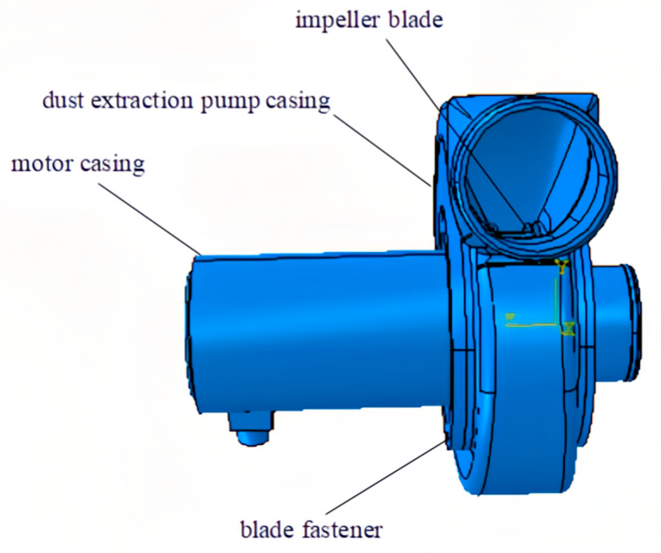
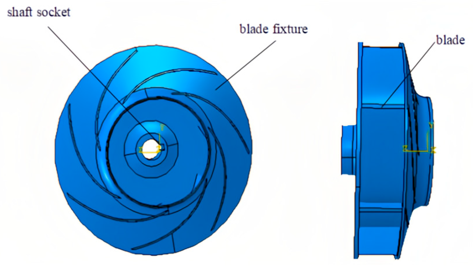
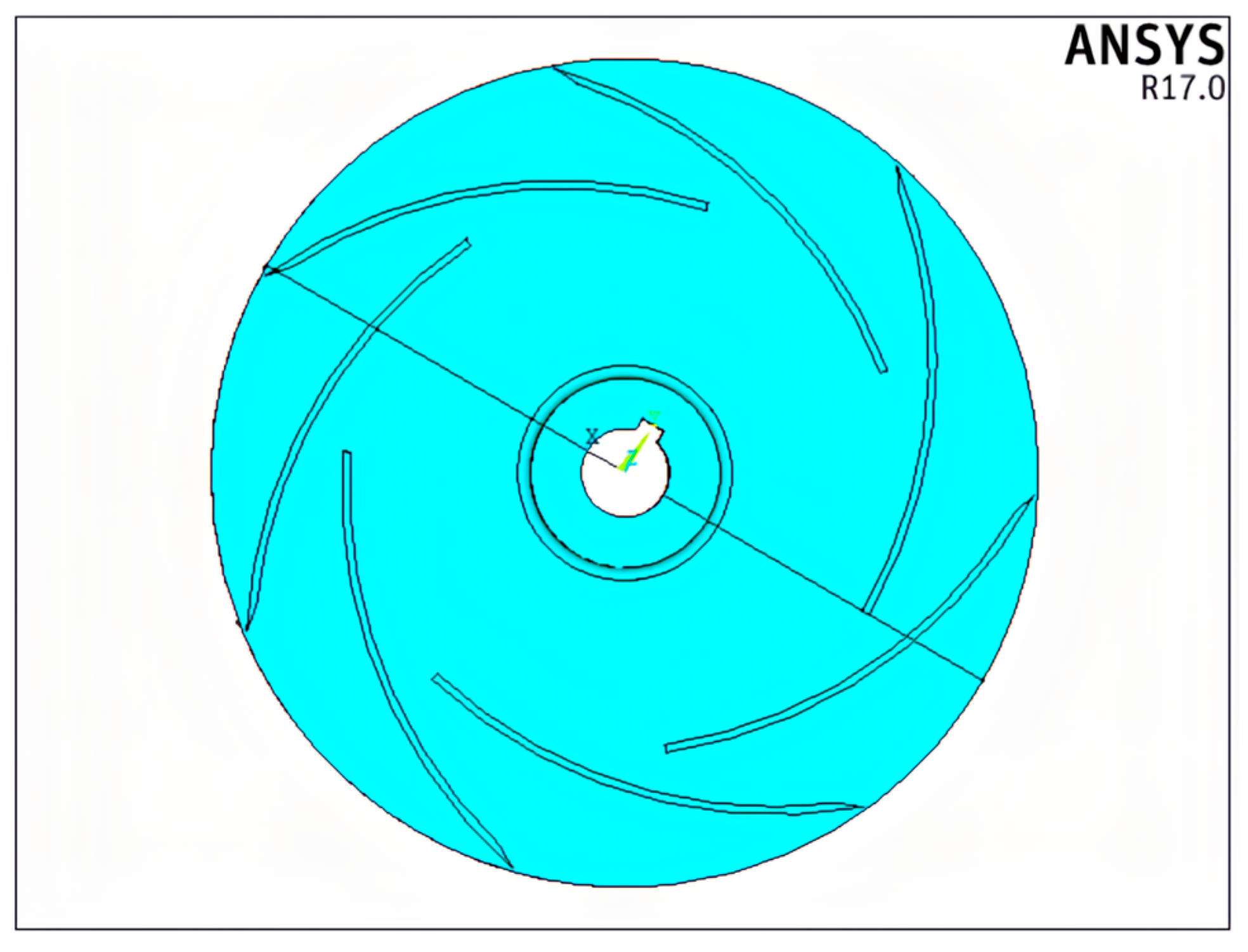
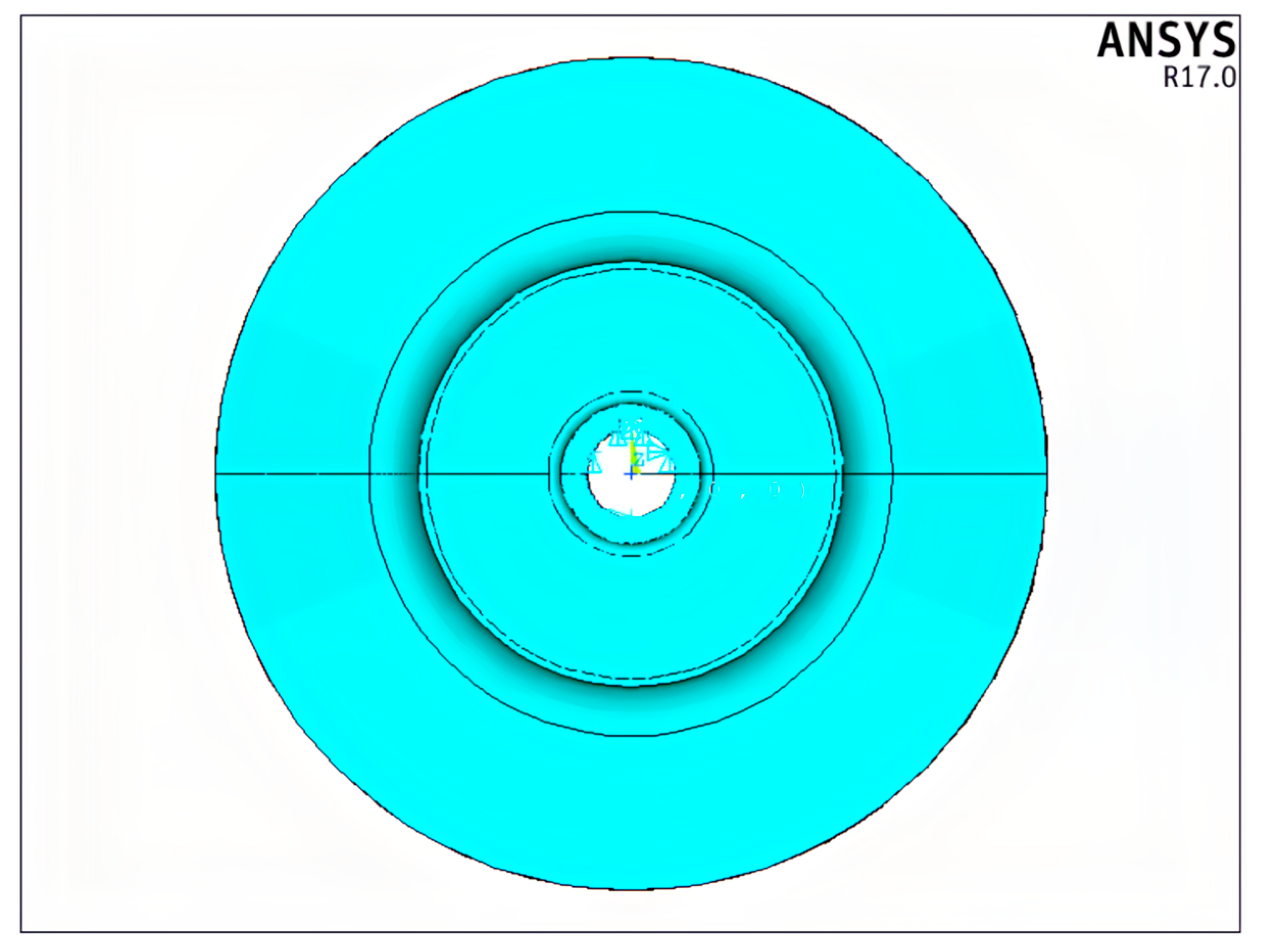
2.1.1. Geometric Model

A dust extraction fan is a type of impeller that comprises multiple components, including a fan casing, impeller fixture, impeller blades, motor casing, and blade fasteners. The fan unit is shown in Figure 1. The fan casing, which is made of rolled steel plates, primarily serves as the structural support, whereas the impeller shown in Figure 2 is a critical component that rotates at approximately 12,500 rpm. Notably, the typical working environment of a dust extraction fan includes extremely high-dust concentrations that can cause significant blade wear that in turn reduces reliability. In addition, considering the statistical uniformity of particle erosion wear when the blades rotate at high speeds in a high-dust environment, this study assumes that the blade thickness decreases uniformly along the circumferential and radial directions [23,24]. Therefore, this study focused on the reliability of the impeller blades.

The impeller parameters are defined in

Table 1. Impeller parameters.

Parameter	Value
Elastic modulus	210 GPa
Poisson’s ratio	0.3
Density	7.85 t/m3
Yield strength	235 MPa
Impeller outer diameter	130 mm
Lower impeller fixture inner hole diameter	14 mm
Upper impeller fixture hole diameter	64 mm
Blade thickness	1 mm
Upper impeller fixture thickness	2 mm
Lower impeller fixture thickness	2 mm
Blade spline width	4 mm
Blade spline depth	2 mm
Blade spline length	12 mm

. The fan casing and impeller components were made of steel with an elastic modulus of E = 210 GPa, Poisson’s ratio of 0.3, density of 7.85 t/m³, and yield strength of 235 MPa. The assembled impeller fixture had an outer diameter of 130 mm and an inner diameter of 14 mm.

A bottom-up approach using the ANSYS Parametric Design Language (APDL) was employed to model the impeller, which consisted of upper and lower fixtures with blades between. The profiles of the two fixtures were first established by setting key points to define the corner positions and connecting these points into closed curves. These curves were subsequently rotated by 360° to form solid fixtures, as shown in Figure 3. The blades were constructed by extruding side profile curves from a blade curve library to form solid bodies. Finally, the blades were arrayed around the center of the bottom fixture at intervals of 53°, as shown in Figure 4. Since the upper fixture had a curved surface, Boolean operations were used to remove any excess portions of the blades protruding through it.

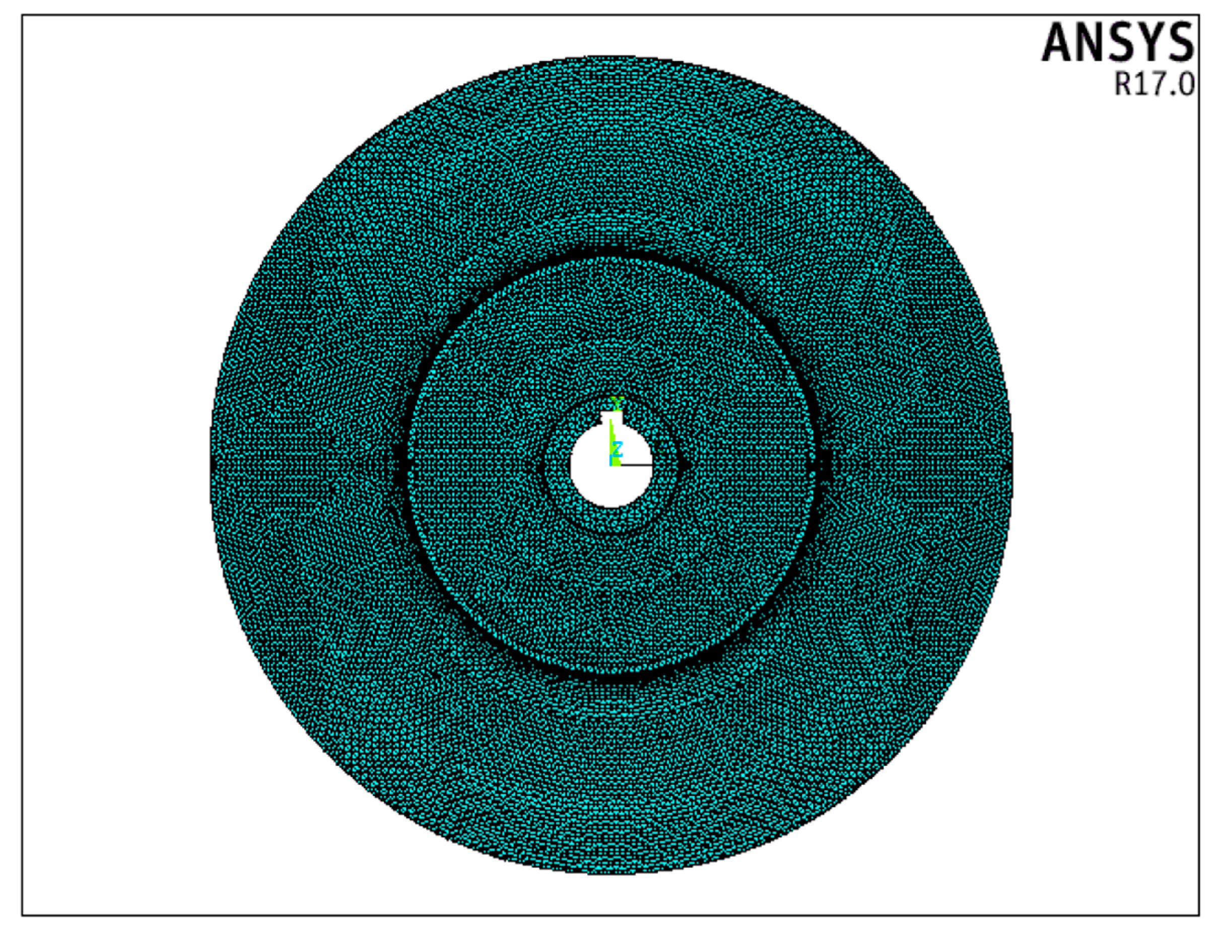
2.1.2. Mesh Generation

The model mesh was divided into tetrahedral and hexahedral SOLID187 elements through mesh generation. Although smaller mesh sizes and higher mesh densities generally lead to higher computational accuracy, an excessive mesh density can significantly increase the computational costs in practical engineering applications. Therefore, the mesh density is considered optimal when further increases in density no longer significantly affect the accuracy of the results. In this study, the impeller model was meshed using 400,953 elements and 708,943 nodes, as shown in Figure 5. In Figure 5, the z-axis is the rotation axis. In the boundary conditions, the translational displacements in the x, y, and z directions are restricted, while rotation around the z-axis is allowed.

2.1.3. Boundary Conditions

The boundary conditions were set reasonably to ensure accurate and reliable simulations. As this study focused on the impeller stress and deformation caused by centrifugal forces at high rotational speeds, the translational displacements in the x, y, and z directions were fixed at the center axis hole of the impeller and the rotations in the x and y directions were restricted, allowing the impeller blades to rotate around the z axis at a speed of 12,500 rpm, as shown in Figure 6.

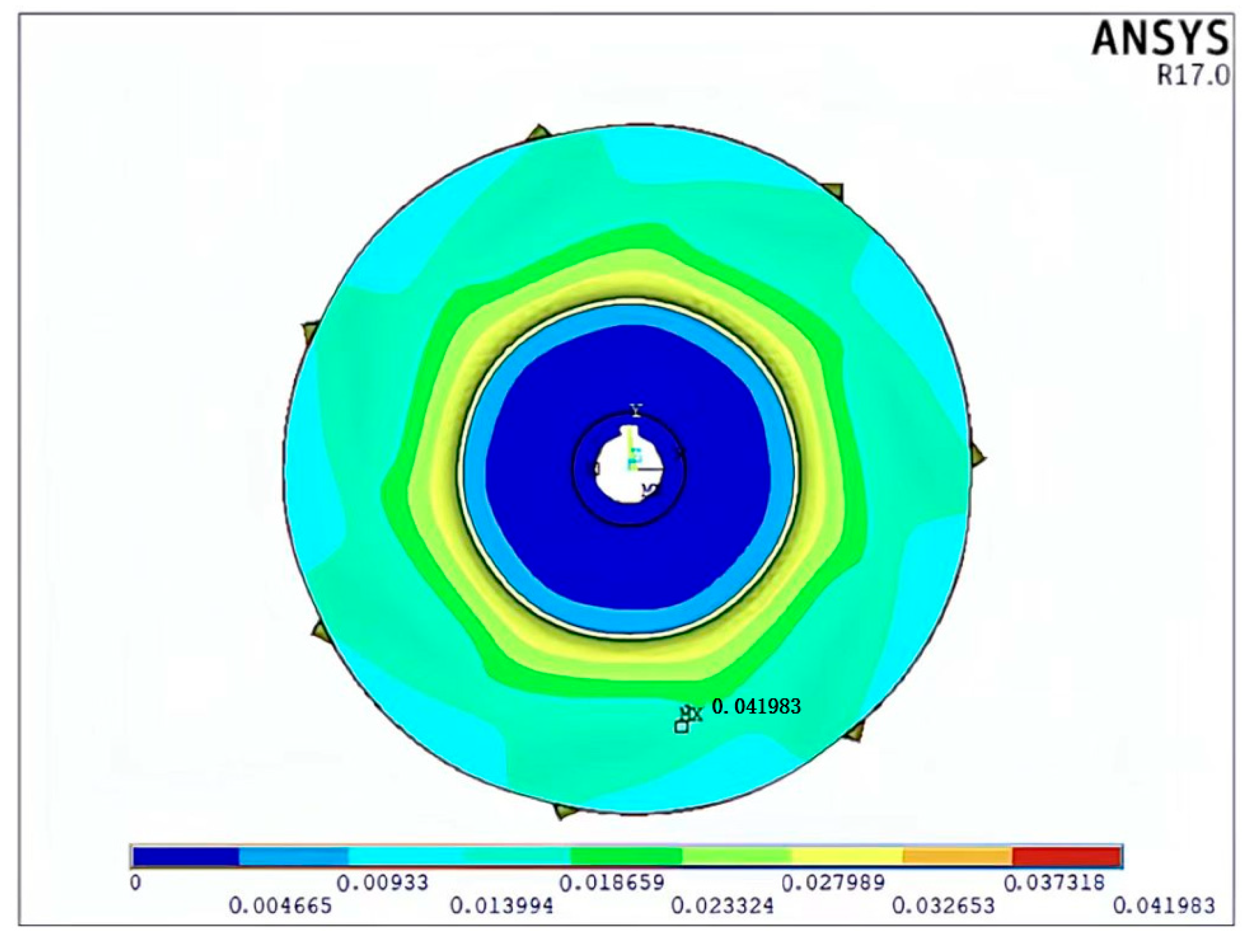
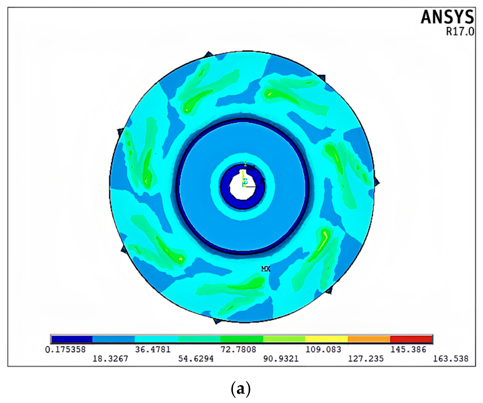
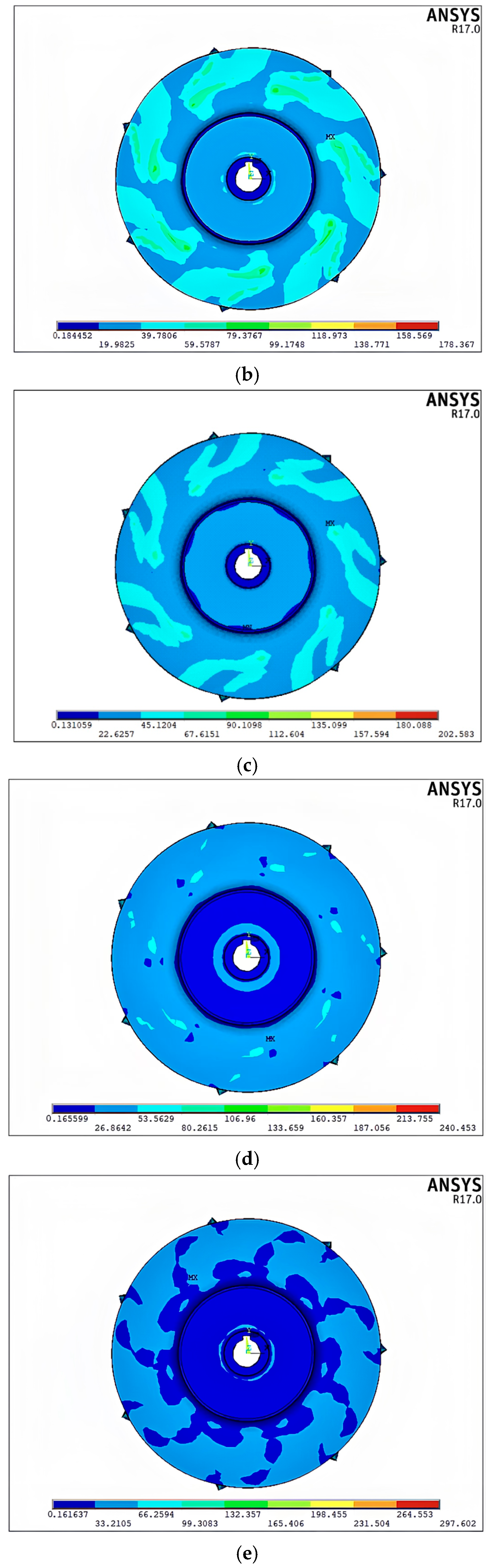
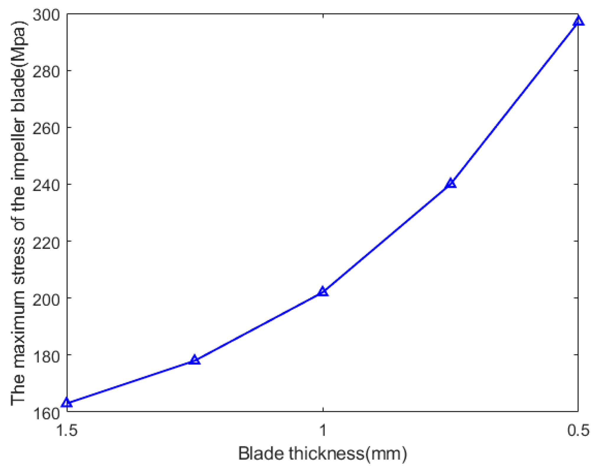
2.1.4. Finite Element Simulation Results

The constructed finite element model was used to determine the stress and displacement contours of the rotating impeller, as shown in Figure 7 and Figure 8, respectively. When the mesh size is selected as 1mm, the entire calculation process takes approximately 120 s.

As shown in Figure 7, the largest impeller deformations typically occurred near the center hole of the upper fixture and midpoints of the blade tips, with a maximum displacement of 0.419 mm. Figure 8 indicates that the high-stress regions were primarily located along the blade roots, where a maximum stress of 178 MPa was observed.

Because impeller failure is primarily caused by significant blade deformation owing to thinning from wear, the finite element simulations were repeated as the blade thickness was gradually reduced from 1.5 mm to 0.5 mm in 0.25 mm increments, yielding the stress contours shown in Figure 9.

The maximum stress in Figure 9a occurred at the root of the impeller blade where it contacts the fixture; the stress in the blade region increased significantly over that in the fixture as the blade thickness decreased in Figure 9b–e, with that at the blade tip increasing constantly once the blade thickness dropped below 1 mm to become the highest-stress region in the entire impeller. These results confirm that the stress in the impeller blades under high-speed rotation increases as the blade thickness decreases.

The relationship between the blade stress and thickness is plotted in Figure 10, which suggests an exponential increase in stress with decreasing thickness; this increase became particularly pronounced once the blade thickness decreased below 1 mm. Indeed, the slope of the stress–thickness curve was approximately 80 when the blade thickness was greater than 1 mm, but it increased to approximately 180 when the thickness was less than 1 mm. This notable change in slope indicates that the rate of increase in blade stress accelerates with blade thinning owing to ongoing wear. Therefore, the blade thickness was set within 0.5–1 mm during the subsequent uncertainty analysis to capture the most vulnerable impeller condition [25].

2.2. Parametric Modeling of Impeller Blades

2.2.1. Selection of Design Parameters

The parameters used to model the deformation and stress in the dust extraction fan blades can be categorized into geometric parameters comprising the fixture and blade thicknesses, material parameters comprising the Poisson’s ratio, elastic modulus, and material density, and loading parameters comprising solely the rotational speed.

Fixture thickness: Because of the limited space within the casing, the sum of the impeller fixture thickness and blade width was held at a constant in this study. Thus, a thicker fixture required a narrower blade width, affecting the blade deformation during rotation. Additionally, the connection between the blade and fixture was set as a tenon joint, which induces stress concentrations at the connection points during rotation.

Blade thickness: The blade thickness inevitably decreases over time with usage. Therefore, the thickness of the impeller blade can vary significantly owing to the conditions in which the dust fan is used. The blade thickness affects the centrifugal force experienced by the blade tip during high-speed rotation, thereby influencing the stress within. Moreover, changes in the blade thickness also affect its stiffness.

Poisson’s ratio: Poisson’s ratio is the ratio of transverse to axial strain in a material under uniaxial tension or compression; it primarily affects the impeller blade deformation.

Elastic modulus: The elastic modulus is a measure of material resistance to elastic deformation. Critically, flaws inherent to the manufacturing process can introduce inhomogeneities into the impeller blade material, and the corresponding variations in the elastic modulus can affect blade deformation.

Material density: Variations in material density owing to the manufacturing process can lead to significant fluctuations in the impeller mass. As this mass affects the centrifugal force experienced by the blades, the material density also influences the stress within.

Rotational speed: The rotational speed is the source of the load applied to the impeller blades. The complex working conditions of vehicles and the high load on their auxiliary systems can cause this rotational speed to vary significantly and rapidly. This uncertainty affects the centrifugal force experienced by the impeller blades, thereby influencing the stress within.

In summary, these material and geometric parameters are subject to uncertainties inherent to the fan manufacturing process and application that can adversely affect the structural reliability of the impeller, and the loading parameters are uncertain owing to the complex working conditions in the vehicle. Therefore, the effects of these six parameters on the blade stress and deformation performance indicators were evaluated using a parametric model.

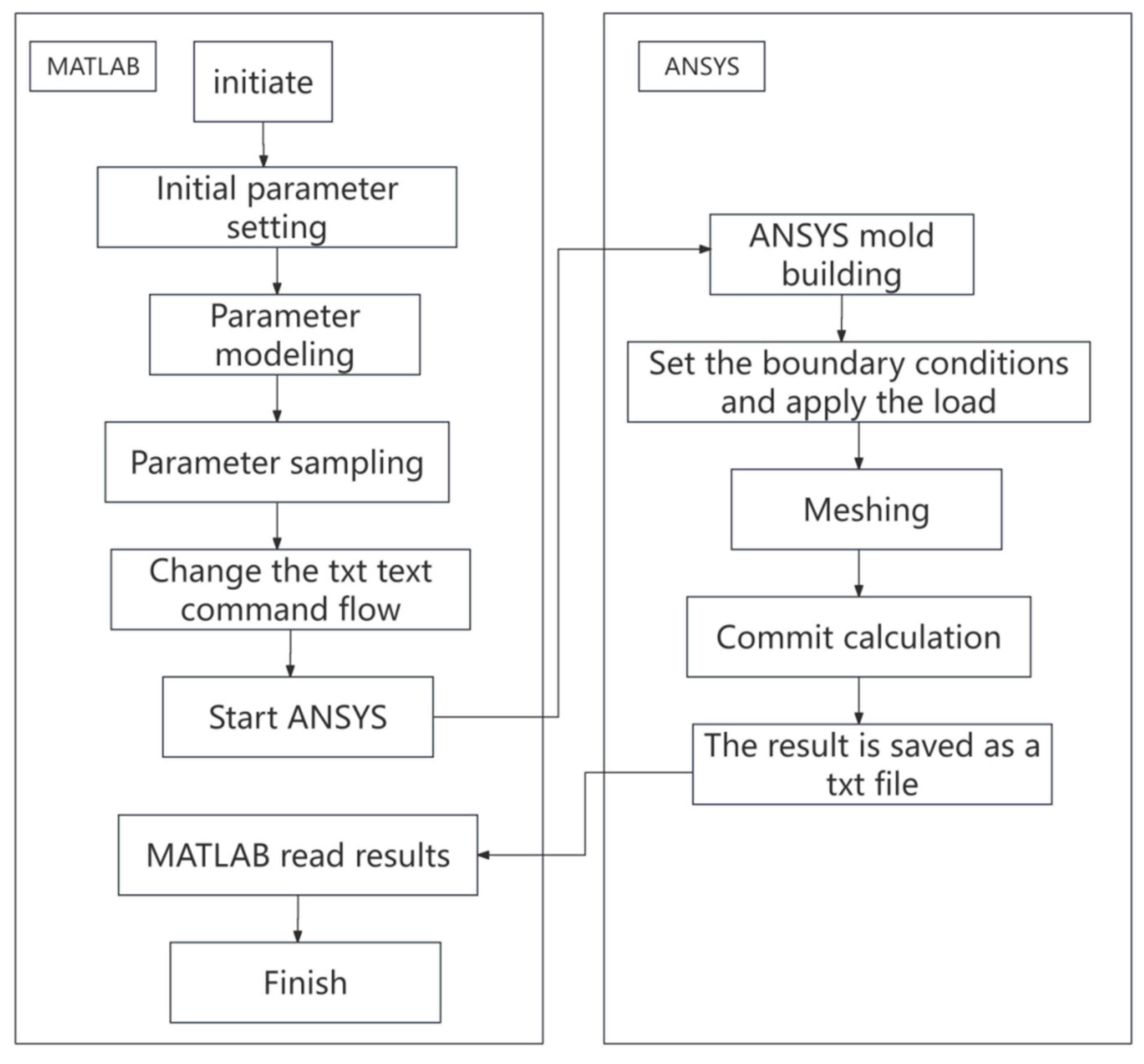
2.2.2. Parametric Modeling

Each command executed in APDL generates a corresponding *.log file that can be directly invoked in subsequent APDL runs. Alternatively, ANSYS R17.0 command streams can be used directly for modeling. This study constructed a deterministic model of the dust extraction fan impeller using the latter approach.

Using APDL alone for the parametric modeling of the dust extraction fan impeller requires significant time for parameterization. During the construction of the deterministic model, the parameters are replaced with letters, which are assigned values at the top of the command stream. Therefore, the MATLAB R2023a software package, which can read text file formats such as .doc, .txt, .k, and .xls, was used to manipulate the parameter information using the “fopen” function to read the established *.txt file, assign the content of this file to the variable “tline”, and then determine the positions of the values to be modified based on their row and column numbers, inserting new data into the positions of the old data. Once this was completed, the *.txt file was saved and closed.

MATLAB R2023a provides convenient means for calling external programs while ANSYS R17.0 provides an interface for external software calls. Therefore, MATLAB R2023a was used to input the modified *.txt file into ANSYS R17.0 for computation. The entire parametric computation process is illustrated in Figure 11. In the ANSYS command stream, the *CFOPEN function was used to create and name a new *.txt file, and the *VWRITE,SMAX (f18.8) function was used to write the simulation results to this file, where “SMAX” denotes the variable name for the output value and (f18.8) specifies the format of the output result. The following MATLAB command was used to invoke ANSYS: %!”ANSYS150.exe”-b-pane3fl -i “ansysinput.txt”-o”result.txt”. In this command, ansysinput.txt is the file containing the command stream and result.txt is the output file that will contain the computation results. After each simulation, the “fopen” function was used again to open the “result.txt” file and read the ANSYS results, completing a single parametric computation.

Geometric and material uncertainties introduced during the impeller manufacturing process and inherent material defects will affect the mechanical performance of the impeller blades. Therefore, the impact of parameter uncertainties on the performance of the impeller blades must be investigated. The parameters varied during the modeling process comprised the fixture thickness, Poisson’s ratio, elastic modulus, blade thickness, density, and rotational speed. Empirical evidence from manufacturing practice suggests that the normal distribution curve is the most widely used theoretical distribution for workpiece errors, and that most natural parameters follow a normal distribution as well. Therefore, the parameters applied in this study were assumed to follow normal distributions [26]. The means and coefficients of variation for these parameter distributions are listed in

Table 2. Impeller blade parameters and their distributions.

Parameter	Distribution	Mean	Coefficient of Variation
Fixture thickness N	Normal	7	0.1
Poisson’s ratio P	Normal	0.3	0.1
Elastic modulus E	Normal	210,000,000,000	0.1
Blade thickness T	Normal	1	0.1
Density D	Normal	7.85 × 10−9	0.1
Rotational speed R	Normal	12,500	0.1

. These values were applied to perform subsequent uncertainty calculations using the distribution functions in MATLAB; the partial sampling and computational results are presented in

Table 3. Partial sampling and computation results.

Sequence	N (mm)	P	E (GPa)	T (mm)	D (t/mm3)	R (r/min)
1	6.838	0.3140	187	0.894	7.025 × 10−9	1290
2	6.647	0.2593	185	1.098	7.330 × 10−9	1364
3	7.735	0.3484	178	0.899	7.143 × 10−9	1600
4	7.601	0.2933	196	0.928	7.596 × 10−9	1248
5	7.610	0.2952	237	1.006	8.024 × 10−9	1319
6	5.928	0.3379	212	0.918	8.719 × 10−9	1647
7	7.610	0.2908	223	1.044	7.676 × 10−9	1173
8	6.462	0.3177	223	1.080	7.493 × 10−9	1340
9	5.885	0.2819	189	1.156	8.053 × 10−9	1273
10	6.908	0.3229	242	0.930	8.148	1364
11	6.462	0.2366	196	0.916	8.976	1600
12	8.673	0.2973	189	0.934	8.477	1248

.

After sampling was completed, the parameter values in the source file (.txt format) were modified using MATLAB R2023a, and then the command stream in the text file was input into ANSYS R17.0 for computation using a batch-processing program. The ANSYS R17.0 software sequentially executed the command stream to complete the four steps of geometric model construction, mesh generation, boundary condition setting, and solution. The results were subsequently output to a *.txt file that was read in MATLAB R2023a, thereby completing a single computation cycle. A total of 500 computation cycles were performed, and the distribution of the results is shown in Figure 12.

Figure 12 shows that when the parameters were sampled according to Table 2, the maximum stress in the impeller blades was distributed in the range [75, 350], with the majority of the data falling within the interval [125, 200].

3. Parameter Response Prediction for Impeller Blades Using Surrogate Models

This study used the feedback neural network, backpropagation neural network, and quadratic response surface methods to establish surrogate models for predicting impeller blade stress based on the input fixture thickness, Poisson’s ratio, elastic modulus, blade thickness, density, and rotational speed parameter values.

3.1. Impeller Blade Stress Prediction Based on Feedback Neural Network

3.1.1. Principle of Feedback Neural Network

Feedback neural networks (FNNs) have strong computational capabilities and can perform efficient calculations without requiring large numbers of network layers or parameters. This characteristic makes FNNs particularly conducive to lightweight modeling applications [27,28]. Similarly to feed-forward propagation, two values are first defined in an FNN:

$${\delta }_h^{H1}={\displaystyle \frac{\partial L}{\partial a_h^{H1}}}$$

(1)

$${\delta }_h^{H1}={\displaystyle \frac{\partial L}{\partial a_h^{H1}}}$$

(2)

where ${\delta }_h^{H1}$ is the error of the output layer, L is the loss function, $a_h^{H1}$ is the activation value of the first-hidden layer, ${\delta }_k$ is the error term of the output layer, calculated as the difference between the true output value T and the model-computed value Y, and a_k is the activation value of the output layer.

The FNN feedback algorithm decomposes the error layer by layer, with each layer connected only to the following layer. Therefore, each layer can be assumed to represent the previous output layer; the error between these layers is used to update the model weights, and the gradient of the current layer’s output with respect to the error can be obtained as a product of the error of the next layer, the weights, and the gradient of the output value as follows:

$${\delta }_h^{H1}={\delta }_k\times {\displaystyle \sum W_{hk}\times f\left(a_h^{H1}\right)}={\displaystyle \sum W_{hk}\times {\delta }_k\times f\left(a_h^{H1}\right)}$$

(3)

where W_hk is the weight matrix connecting the current layer to the next layer and f($a_h^{H1}$) is the derivative of the activation function applied to the activation value $a_h^{H1}$ of the first hidden layer.

Note that if ${\delta }_k$ on the right side of Equation (2) is for the output layer, the gradient can be directly calculated using Equation (2); if ${\delta }_k$ is for a non-output layer, the gradient must be obtained through a feedback approach. A more generalized expression for Equation (2) can be written as follows:

$${\delta }^l={\displaystyle \sum W_{ij}^l\times {\delta }_j^{l+1}\times f^{\prime }\left(a_i^j\right)}$$

(4)

where $W_{ij}^l$ is the weight matrix connecting layer l to layer l + 1, ${\delta }_j^{l+1}$ is the error term of layer l + 1, and $f^{\prime }\left(a_i^j\right)$ is the derivative of the activation function.

This generalized equation can be manipulated to transform the gradient calculation of the current layer’s output with respect to its input into a gradient calculation for the next layer.

The purpose of FNN computation is similar to that of gradient descent, which is to update the model weights. Weight updating in an FNN can be performed in a manner similar to gradient descent weight updating as follows:

$$W_{ji}=W_{ji}+\alpha \times {\delta }_j^l\times x_{ji}$$

(5)

$$b_{ji}=b_{ji}+\alpha \times {\delta }_j^l$$

(6)

where a denotes the learning rate, x denotes the input value to the neuron in the current layer, b denotes the bias term of the neuron, ji represents the node coefficients during backpropagation, and the weights are updated through the calculation of ${\delta }_j^l$.

The FNN receives information from the hidden layer through the connection layer and then sends the output of the hidden layer from the previous time step and the input from the current time step to the hidden layer.

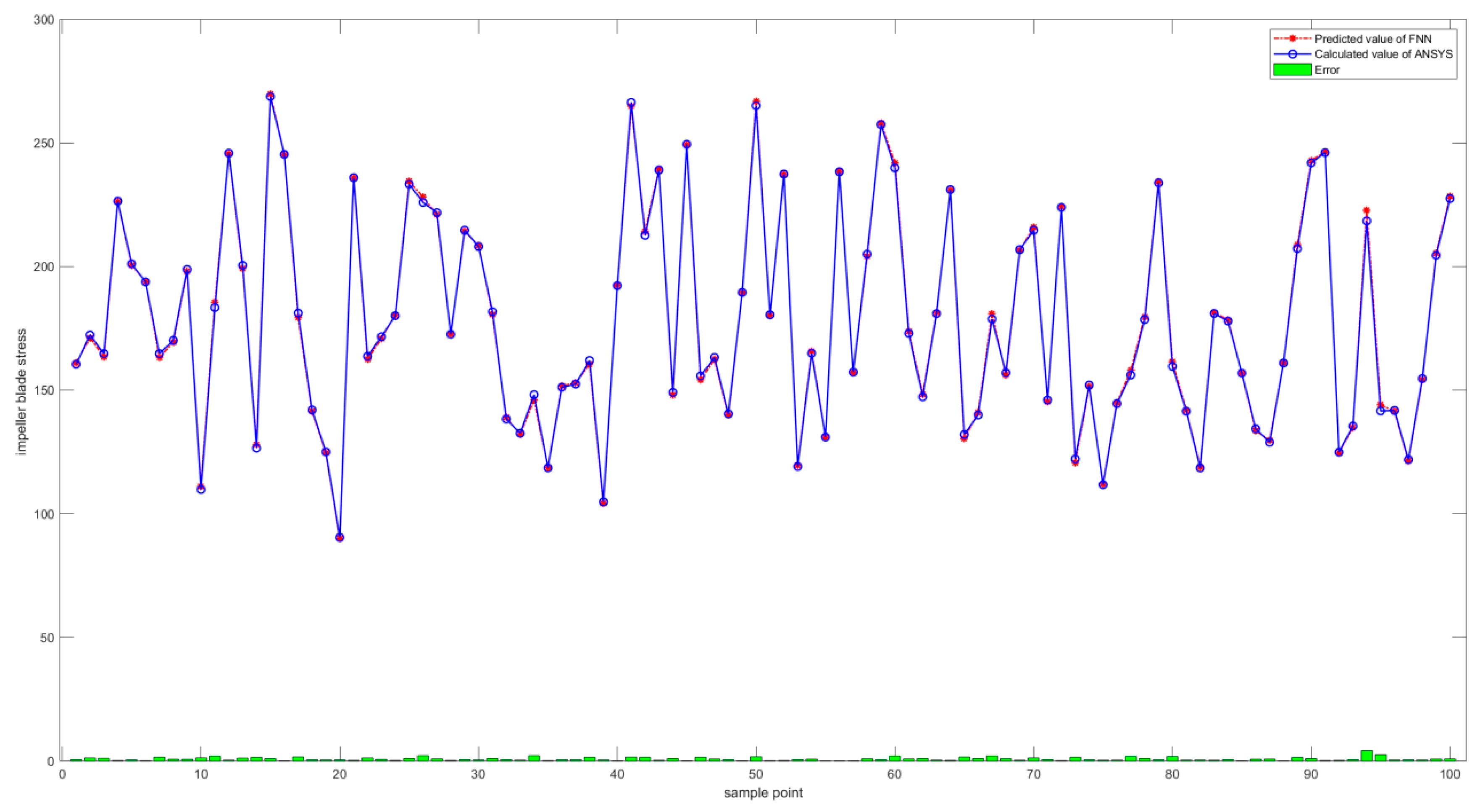
3.1.2. FNN Stress Predictions

The FNN was trained to predict stresses in the impeller blades based on different parameter values using the following process.

Step 1: Based on the mean values and coefficients of variation for the six considered parameters, 500 sets of samples (N) were generated to serve as the FNN input. The input set T was defined as

$$T=\left\{N_{HK},P_{HK},E_{HK},T_{HK},D_{HK},R_{HK}\right\},H=1,2,\dots ,450,K=1,2,\dots ,6$$

(7)

where the subscript H represents the number of rows in the dataset and the subscript K represents the number of columns in the dataset, reflecting the number of parameters considered. The set T was divided into a training set T₁ containing N₁ samples and a testing set T₂ containing N₂ samples, where N₁ + N₂ = 500.

Step 2: ANSYS was applied to calculate the maximum stress in the impeller blades for each set of data and then it was recorded in response to set I. Similarly to Step 1, this response set was divided into training set I₁ and testing set I₂, where I₁ + I₂ = 500.

Step 3: The “Elment” function in MATLAB was used to create an FNN and train it using training set T₁ from Step 1 as the input and response set I₁ from Step 2 as the output. The FNN was designed with three hidden layers, each containing 45 neurons. The maximum number of iterations for the FNN was set to 5000, and the initial learning rate was set to 0.2. The training process began by learning the nonlinear mapping relationships between the input parameters and corresponding impeller blade stress output.

Step 4: Finally, the testing set T₂ from Step 1 was input into the trained FNN to calculate the output $I_2^{\prime }$ and determine the predictive accuracy Pr of the FNN relative to I₂ as follows:

$$\mathrm{Pr}={\displaystyle \frac{\left|I_2-I_2^{\prime }\right|}{I_2}}$$

(8)

The resulting stress prediction errors obtained by the FNN are shown for 100 sample points in Figure 13.

The blue line in Figure 13 represents the stress calculated by ANSYS R17.0, the red line represents the stress predicted by the FNN, and the green bars represent the errors between these two results. Clearly, the blue and red lines are nearly coincident, indicating that the FNN exhibited strong learning capabilities. Indeed, the magnitude of the maximum absolute error between the output and actual values was 3.34 MPa, corresponding to a maximum error of 1.25% and an average error of 0.43%. Therefore, the FNN effectively captured the relationship between the impeller blade parameters and stress.

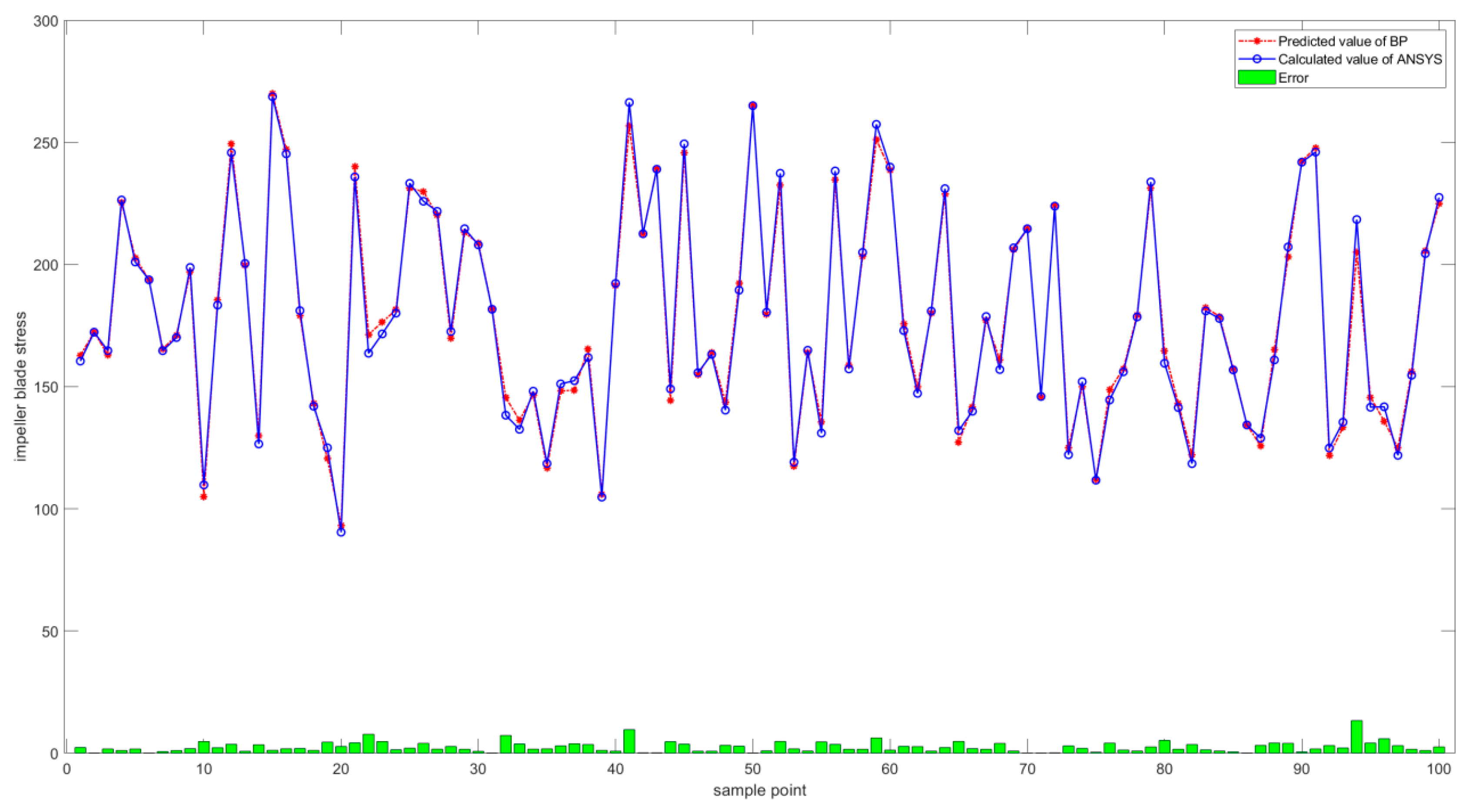
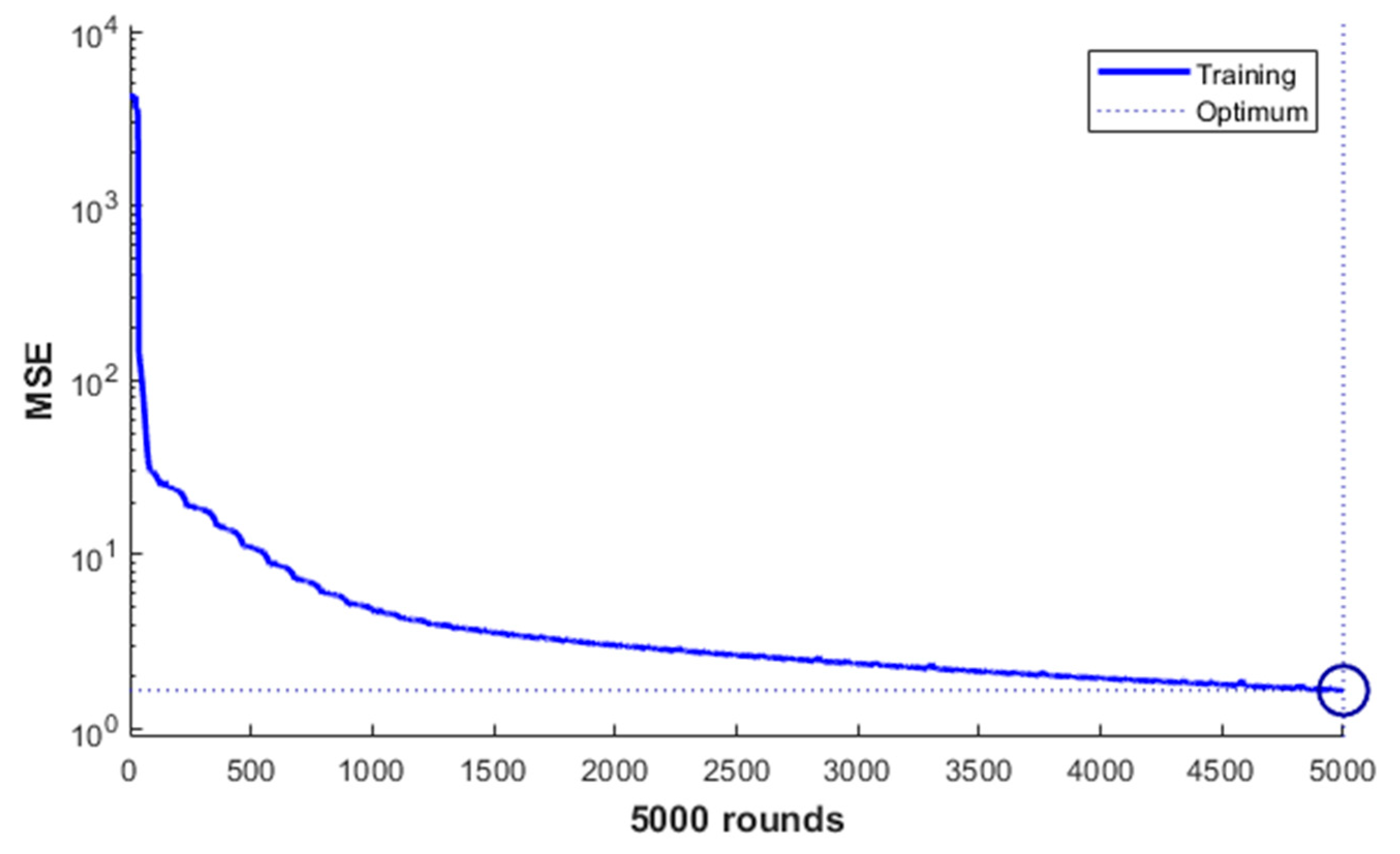
3.2. Impeller Blade Stress Prediction Based on Backpropagation Neural Network

3.2.1. Principle of Backpropagation Neural Network

The backpropagation neural network (BPNN) was proposed by Rumelhart and McClelland in 1986. It comprises a multiple-layer feed-forward neural network that propagates errors backward to realize strong nonlinear fitting capabilities [29].

3.2.2. BPNN Stress Predictions

The following process was used to construct the BPNN evaluated in this study:

Step 1: The 500 sets of parameter data sampled by MATLAB R2023a and stress results calculated by ANSYS R17.0 were combined into a sample set that was divided into a training set containing the first 400 samples and a testing set containing the remaining 100 samples.

Step 2: The number of layers and nodes in each layer of the BPNN were determined, and the weights and thresholds for each layer were initialized. A three-layer BPNN was constructed in this study with the input layer containing 14 nodes representing the fixture thickness, Poisson’s ratio, elastic modulus, blade thickness, density, and rotational speed and the output layer containing one node representing the stress in the impeller blade under load. The number of nodes in the hidden layer was determined as follows:

$$h=\sqrt{m+n}+a$$

(9)

where h is the number of nodes in the hidden layer, m is the number of input layer nodes (5), n is the number of output layer nodes (1), and a is a value between 1 and 10. The “tansig” transfer function was used between the first and second hidden layers, the “purelin” transfer function was used between the second and third hidden layers, and the “TrainLM” function was used for training

Step 3: The number of training iterations, learning rate, and minimum error target for training were determined.

Step 4: Four convergence conditions were set to avoid overfitting: the number of training iterations, training time, generalization ability, and error precision. These convergence conditions were defined as follows: the number of training iterations was limited to 10,000, the error precision was set less than $0.65\times {10}^{-3}$ and training was stopped if the error did not change for six consecutive iterations, and training time was limited to one minute. Training was terminated once any of these conditions was met.

Step 5: The errors between the actual output and correct values were calculated as follows:

$$Err={\displaystyle \frac{\left|T_a-T_n\right|}{T_a}}$$

(10)

The stress prediction errors obtained by the BPNN are presented for 100 sample points in Figure 14.

The blue line in Figure 14 represents the stresses calculated by ANSYS, the red line represents the stresses predicted by the BPNN, and the green bars represent the errors between these two results. The curves of the calculated and BPNN-predicted stresses are nearly coincident, with a maximum error of 14.83% occurring at sample point 94. The remaining errors were less than 10% with an average value of 1.79%. The training performance diagram of the backpropagation (BP) neural network is shown in Figure 15, and it can be seen that its convergence is good. These results indicate that the BPNN effectively predicted the impeller blade stress.

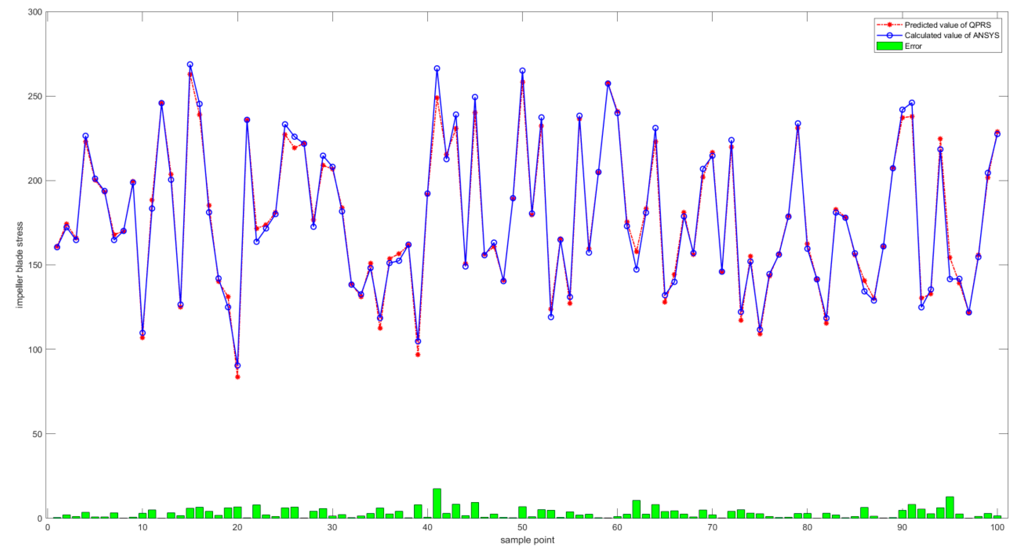
3.3. Impeller Blade Stress Prediction Based on Quadratic Polynomial Response Surface Method

3.3.1. Principle of Quadratic Polynomial Response Surface Method

The convenience of the quadratic polynomial response surface (QPRS) method facilitates its ready application to fit the dust extraction fan impeller blade stress in this study, thereby significantly reducing the computational workload and shortening the reliability analysis cycle. The QPRS method employs a quadratic polynomial function to represent the implicit functional relationship between variables; this is known as the response surface function, and its general form is given by [30].

$$g\left(X\right)={\displaystyle \sum _{i=1}^n{a}_i{x}_i^2+b_i{x}_i+c}$$

(11)

where X represents the experimental data points and a_i, b_i, and c are unknown coefficients, in which i = 1 − n.

Equation (10) indicates that there are 2n + 1 unknown parameters in the response surface function, requiring 2n + 1 sample points to obtain a solution. First, the central data point $X_m$ was determined with its initial value set as the mean of the random vector $X_m={\overline{x}}_i=\left(u_1,u_2,\dots ,u_n\right)$. The surrounding data points were subsequently selected by deviating from this central data point by αs_i (where α is the deviation coefficient and s_i is the standard deviation of the i-th variable; typically, α = 1–3), resulting in expressions for the other experimental points as follows:

$${\overline{x}}_i=\left(u_1,u_2,\dots u_i\pm \alpha s_i,\dots ,u_n\right)$$

(12)

The $g\left(X\right)$ values corresponding to these data points were calculated using ANSYS, and the unknown coefficients in Equation (10) were solved by resolving the determinant to obtain an explicit expression of the implicit function $g\left(X\right)$.

3.3.2. QPRS Stress Predictions

The following process was used to determine the QPRS function:

Step 1: The central point $x^0=\left(x_1^0,x_2^0,\dots ,x_n^0\right)$ was determined and set as the mean value. Six variables were considered in this study, n = 6.

Step 2: Each variable was sequentially deviated from the central point by αs_i using the least squares method, and each resulting vector $x^0$ was placed into the rows of matrix A with dimensions $\left(2n+1\right)\times \left(2n+1\right)$.

Step 3: Finite element calculations of $\widehat{y}\left(x_1^n,x_2^n,\dots ,x_n^n\right)$ were conducted using a total of 2n + 1 computations.

Step 4: The least squares method was employed to solve the unknown coefficients a_i, b_i, and c describing the response surface. The explicit expression obtained by fitting the impeller blade stress using the QPRS method is given by

$$\begin{array}{l}g=-42.42-3.1e^{10}{x}_1-0.000556x_2+0.822x_3-96.16x_4+0.0866x_5-234.88x_6\\ -5.67e^{17}{x}_1^2+1.382e^{-9}{x}_2^2-0.041x_3^2+145.15x_4^2+7.0016e^{-5}{x}_5^2+80.79x_6^2\end{array}$$

(13)

The stress prediction errors obtained by the QPRS method are shown for 100 sample points in Figure 15.

Figure 16 indicates that the fitted polynomial obtained using the QPRS method exhibited a fit accuracy in excess of 90% with a maximum error of 9% and an average error of 1.89%. Figure 17 shows the curve of the mean squared error of the established feedback neural network surrogate model changing with the number of iterations. It can be seen that the training using the feedback neural network has good convergence. Thus, the QPRS method can provide a high-precision surrogate model using a minimal number of sample points.

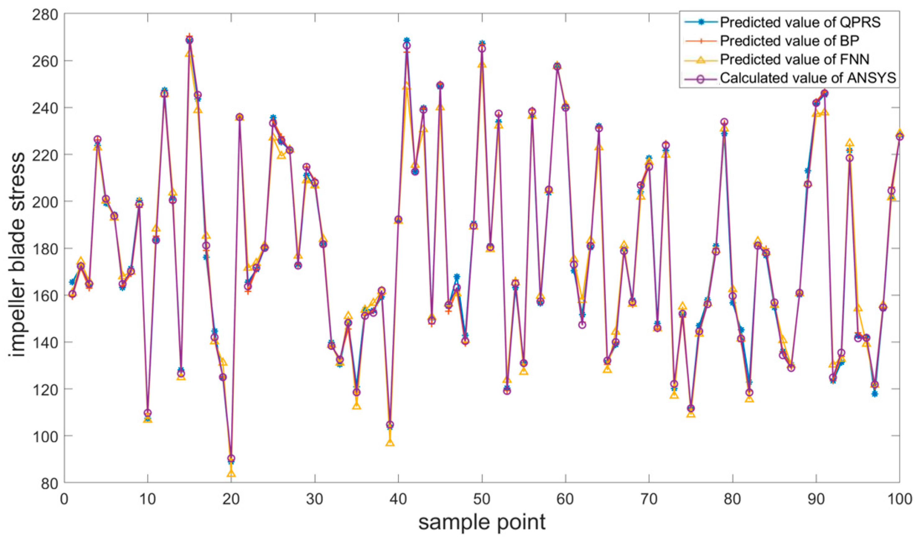
3.4. Comparison of Surrogate Model Performance

The training and validation results obtained using the FNN, BPNN, and QPRS surrogate models to predict the stresses in the impeller blades are compared in

Table 4. Comparison of surrogate model performance.

Model	Training Set Fit	Maximum Stress Error in Test Set	Average Stress Error in Test Set	Training Speed
BPNN	0.99997	0.1483	0.0179	14 s
FNN	0.99973	0.0125	0.0043	9 s
QPRS	0.9378	0.09	0.0189	1 s

and Figure 18, which indicates that the BPNN exhibited the highest training set fit and a low average error of 1.79% but also exhibited the highest maximum error of 14.79%. The FNN exhibited a slightly lower training set fit with a much smaller average error of 0.43% and maximum error of only 1.25%. This indicates that the FNN effectively reflected the relationship between the impeller blade parameters and stress. Finally, the QPRS fit exhibited the poorest overall performance among the three considered indicators with the lowest fit and highest average error. Therefore, the FNN was identified as the best choice for determining the optimal parameters of a dust extraction fan impeller. The above calculations were performed using an AMD Ryzen 9 3950X 16-Core Processor (Advanced Micro Devices, Santa Clara, CA, USA).

4. Conclusions

The dust extraction fan is a core component that determines the performance of the vehicle filtration system. During vehicle operation, the impeller blades of the dust extraction fan rotate at a high speed in extremely dusty environments, subjecting them to continuous wear. As failure of the dust extraction fan can lead to filter clogging, reduced engine thermal efficiency, and engine “scuffing” problems, this study established a parametric model of the fan impeller to perform reliability analyses using different surrogate models. The primary conclusions of this study are as follows:

(1)

The structural characteristics and load conditions of the impeller were analyzed in detail to clarify the constraints and loads it experiences during service. The stress and displacement distributions in impeller blades with different thicknesses were determined through a series of finite element analyses considering the appropriate material property definitions, mesh generation, constraint conditions, and load application. The most critical location on the impeller blade was determined to be the midpoint of the blade tip, where the maximum displacement was observed.

(2)

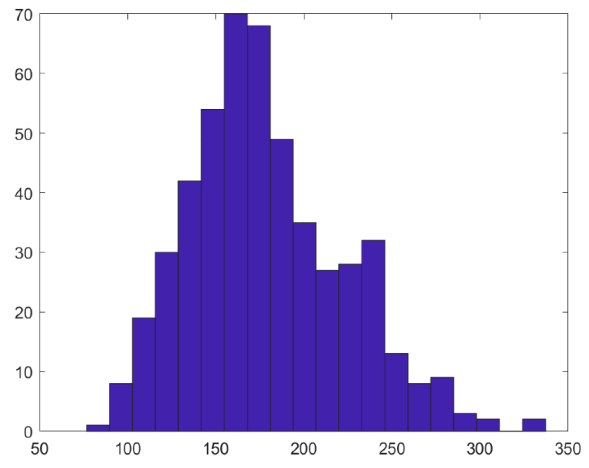
The FNN, BPNN, and QPRS surrogate models were constructed to predict the impeller blade stress based on the input parameters. Six random variables were selected as the inputs to each model, and the maximum stress in the impeller blades was considered the output. MATLAB R2023a software was used to construct training samples based on the distribution of each parameter, and a parametric model was established using APDL to conduct batch calculations. After these calculations were completed, the parameter values and corresponding stresses were combined into a training set to train each surrogate model. Among the three considered surrogate models, the FNN exhibited the smallest prediction error of 0.0043.

The results of this study demonstrate the utility of using an FNN as a surrogate model in place of a detailed finite element analysis when evaluating the reliability of dust extraction fans, thereby reducing computational costs and improving efficiency while ensuring accuracy.

The main contribution of this paper is that a comparative study of multi-agent models is carried out for the dust-absorbing fan impeller, which identifies the advantages of the FNN in predicting the stress response of the impeller and provides an efficient and accurate method for reliability analysis in this field. This not only helps to promote the development of vehicle filtration system reliability research but also provides theoretical support and technical guarantee for the safe and stable operation of vehicles in complex environments.

Despite the results achieved in this study, there are still limitations. From the perspective of numerical methods, although agent models such as the FNN perform well in prediction accuracy, the prediction results may be biased when dealing with certain parameter combinations under extreme working conditions. This is because the complexity of the actual working conditions is far beyond the scope of model training, and some rare parameter combinations may exceed the learning ability of the model. In addition, model training relies on a large amount of sample data, and the quality and quantity of the data directly affect model performance. If the data are biased or insufficient, this will lead to a decrease in the generalization ability of the model.

To address these shortcomings, in the future, we can try to introduce the migration learning technique, which utilizes the model parameters that have been trained in similar fields and combines the small number of data in this study to fine-tune them, so as to improve the adaptability of the model under extreme working conditions. At the same time, the data collection strategy should be optimized to increase the diversity and representativeness of the samples, or data enhancement techniques should be used to expand the training data.

References

1. Chen, Y.; Cai, Y.; Yang, G.; Zhou, H.; Liu, J. Neural adaptive pointing control of a moving tank gun with lumped uncertainties based on dynamic simulation. J. Mech. Sci. Technol. 2022, 36, 2709–2720. [Google Scholar] [CrossRef]
2. Lu, J.; Xie, D.; Wang, J.; Sun, Y.; Qiao, M.; Li, J.; Li, W.; Chen, K. Experimental Study on the Air Filter of a Heavy Vehicle in Desert Areas. Veh. Power Technol. 2016, 3, 16–20. [Google Scholar]
3. Rivera, B.H.; Rodriguez, M.G. Characterization of Airborne Particles Collected from Car Engine Air Filters Using SEM and EDX Techniques. Int. J. Environ. Res. Public Health 2016, 13, 985. [Google Scholar] [CrossRef] [PubMed]
4. Song, X. Performance Analysis and Structural Optimization of the Air Filter of a Heavy Truck Based on Fluid-Structure Interaction. Master’s Thesis, Qilu University of Technology, Jinan, China, 2023. [Google Scholar]
5. Zhang, J.; Guo, Z.; Zhang, H.; Wang, X. Flow Field Analysis and Structural Optimization of the Air Filter of a Vehicle Diesel Engine. Intern. Combust. Engines 2023, 39, 26–32. [Google Scholar]
6. Hu, T. Discussion on the Performance Testing Method of Motorcycle Air Filters. Motorcycle Technol. 2005, 7, 25–26+48. [Google Scholar]
7. Lu, J.; Sun, Y.; Qiao, M.; Wang, J.; Chen, K. Simulation and Experimental Study on the Performance of Air Filter Filter Materials. Veh. Power Technol. 2019, 1, 38–42+49. [Google Scholar]
8. Sun, Y.; Wang, J.; Lu, J.; Qiao, M.; Chen, K.; Li, W.; Li, J. Research on a Simulation Analysis Method of Air Filters. Veh. Power Technol. 2014, 3, 32–34+49. [Google Scholar]
9. Hao, Y. Analysis of the Force-Thermal Coupling Response of Turbine Blades. Master’s Thesis, Beijing University of Chemical Technology, Beijing, China, 2023. [Google Scholar]
10. Tang, Y. Point Cloud Denoising and Surface Reconstruction in the Preparation of Turbine Blades Based on Deep Learning. Master’s Thesis, Southwest University of Science and Technology, Langfang, China, 2023. [Google Scholar]
11. Li, Y.; Qin, Q.; Wang, Y.; Hu, M. Welded Joint Fatigue Reliability Analysis on Bogie Frame of High-Speed Electric Multiple Unit. J. Shanghai Jiaotong Univ. (Sci.) 2017, 22, 365–370. [Google Scholar] [CrossRef]
12. Gao, W.; Mo, X.; Fu, R.; Sun, G. 6σ Robust Optimization Design of the Crashworthiness of Foam-Filled Conical Thin-Walled Structures Based on Kriging. Acta Mech. Solida Sin. 2012, 33, 370–378. [Google Scholar]
13. Gupta, S.; Manohar, C.S. Improved response surface method for time-variant reliability analysis of nonlinear random structures under non-stationary excitations. Nonlinear Dyn. 2004, 36, 267–280. [Google Scholar] [CrossRef]
14. Zhang, C.; Bai, G.; Xiang, J. Reliability Optimization Design of Flexible Mechanisms Based on the Extreme Value Response Surface Method. J. Harbin Eng. Univ. 2010, 31, 1503–1508. [Google Scholar]
15. Kang, Z.; Luo, Y. Reliability-based structural optimization with probability and convex set hybrid models. Struct. Multidiscip. Optim. 2010, 42, 89–102. [Google Scholar] [CrossRef]
16. Ling, J.; Kurzawski, A.; Templeton, J. Reynolds averaged turbulence modelling using deep neural networks with embedded invariance. J. Fluid Mech. 2016, 807, 155–166. [Google Scholar] [CrossRef]
17. Ladický, L.U.; Jeong, S.; Solenthaler, B.; Pollefeys, M.; Gross, M. Data-driven fluid simulations using regression forests. ACM Trans. Graph. 2015, 34, 1–9. [Google Scholar] [CrossRef]
18. Milani, P.M.; Ling, J.; Eaton, J.K. Physical interpretation of machine learning models applied to film cooling flows. J. Turbomach. 2019, 141, 011004. [Google Scholar] [CrossRef]
19. Maral, H.; Şenel, C.B.; Deveci, K.; Alpman, E.; Kavurmacıoğlu, L.; Camci, C. A genetic algorithm based multi-objective optimization of squealer tip geometry in axial flow turbines: A constant tip gap approach. J. Fluids Eng. 2020, 142, 021402. [Google Scholar] [CrossRef]
20. Zhang, L.; Sun, X.; Chen, J.; Sun, Y.; Guo, J.; Zheng, J. Research Progress in Reliability Analysis and Optimal Design of Automobile Structures. China Mech. Eng. 2024, 35, 1948–1962. [Google Scholar]
21. Roccia, B.A.; Ruiz, M.; Gebhardt, C.G. On the use of feed-forward neural networks in the context of surrogate aeroelastic simulations. Acta Mech. 2025, 236, 673–705. [Google Scholar] [CrossRef]
22. Awad, A.N.; Jarad, T.S. Hybrid Particle Swarm Optimization and Feedforward Neural Network Model for Enhanced Prediction of Gas Turbine Emissions. Int. J. Energy Prod. Manag. 2024, 9, 97–105. [Google Scholar] [CrossRef]
23. Ma, C.; Wang, N.; Guo, S.; Wang, R. Numerical Simulation of the Performance Deterioration of a Radial Flow Turbine Caused by Particle Erosion. Trans. CSICE 2024, 42, 358–366. [Google Scholar] [CrossRef]
24. Singh, G. Effect of suspended particles on erosion characteristics of impeller steels utilizing combined CFD and DOE approach. Ind. Lubr. Tribol. 2025, 77, 202–210. [Google Scholar] [CrossRef]
25. Wang, L.-F.; Zhou, X.-P. A field-enriched finite element method for simulating the failure process of rocks with different defects. Comput. Struct. 2021, 250, 106539. [Google Scholar] [CrossRef]
26. Fan, Z. Research on the Distribution Law of NC Machining Precision. Ph.D. Thesis, Northeastern University, Shenyang, China, 2013. [Google Scholar]
27. Liu, L.; Zhong, L. Research on the Thermal Shock Resistance of the Fuselage Coating Based on the Feedback Neural Network. Ordnance Mater. Sci. Eng. 2023, 46, 106–111. [Google Scholar]
28. Yan, H. Coal gangue image classification model based on the improved feedback neural network. Ind. Mine Autom. 2022, 48, 50–55+113. [Google Scholar]
29. Mohamad, E.T.; Faradonbeh, R.S.; Armaghani, D.J.; Monjezi, M.; Majid, M.Z.A. An optimized ANN model based on genetic algorithm for predicting ripping production. Neural Comput. Appl. 2017, 28, 393–406. [Google Scholar] [CrossRef]
30. Shan, D.; Li, Q.; Khan, I.; Zhou, X. A novel finite element model updating method based on substructure and response surface model. Eng. Struct. 2015, 103, 147–156. [Google Scholar] [CrossRef]
Figure 1. Dust extraction fan model.
Machines 13 00496 g001
Figure 2. Dust extraction fan impeller model.
Machines 13 00496 g002
Figure 3. Model constructed using APDL.
Machines 13 00496 g003
Figure 4. Blade model constructed using APDL.
Machines 13 00496 g004
Figure 5. Mesh of impeller model (looking down onto the upper fixture).
Machines 13 00496 g005
Figure 6. Model boundary conditions (looking down onto the upper fixture).
Machines 13 00496 g006
Figure 7. Displacement contour of the rotating impeller (looking down onto the upper fixture).
Machines 13 00496 g007
Figure 8. Stress contour of the rotating impeller (looking down onto the upper fixture).
Machines 13 00496 g008
Figure 9. Stress contours obtained for blade thicknesses of (a) 1.5 mm, (b) 1.25 mm, (c) 1.00 mm, (d) 0.75 mm, and (e) 0.50 mm (looking down onto the upper fixture).
Machines 13 00496 g009aMachines 13 00496 g009b
Figure 10. Blade stress according to blade thickness during wear.
Machines 13 00496 g010
Figure 11. Workflow of joint ANSYS–MATLAB computation.
Machines 13 00496 g011
Figure 12. Distribution of ANSYS computation results.
Machines 13 00496 g012
Figure 13. Stress prediction errors obtained by the trained FNN.
Machines 13 00496 g013
Figure 14. Stress prediction errors obtained by the trained BPNN.
Machines 13 00496 g014
Figure 15. The training performance diagram of the BP neural network.
Machines 13 00496 g015
Figure 16. Stress prediction errors obtained by QPRS fitting.
Machines 13 00496 g016
Figure 17. The training performance diagram of the FNN.
Machines 13 00496 g017
Figure 18. Comparison of the output results of the three models.
Machines 13 00496 g018