Vision-Guided Fuzzy Adaptive Impedance-Based Control for Polishing Robots Under Time-Varying Stiffness

Abstract

Robotic polishing is crucial for achieving superior surface finishes in manufacturing. However, precise force control presents significant challenges, particularly for curved workpieces exhibiting time-varying stiffness. Traditional methods typically struggle to adapt to these dynamic conditions, often leading to inconsistent results and suboptimal surface quality. This study proposes an Adaptive Impedance Control based on Visual Guidance (AICVG) strategy for robotic polishing. This approach integrates real-time visual feedback for geometric perception and adaptive tool path generation with a fuzzy logic system that dynamically adjusts impedance parameters to account for unforeseen surface stiffness variations. Simulations and experimental validations conducted on a robotic platform demonstrate that the AICVG strategy significantly outperforms both traditional impedance control and conventional fuzzy logic-based adaptive impedance control. Specifically, it maintains force control errors within ±1.5 N under dynamic stiffness conditions and achieves a 60% reduction in workpiece surface roughness compared to the aforementioned alternative methods. This study presents a robust and precise control framework that significantly enhances the adaptability and efficacy of robotic polishing for complex geometries, thereby advancing automated solutions in high-precision manufacturing.

1. Introduction

Polishing represents a critical manufacturing process, particularly for curved workpieces [1,2,3]. This process aims to enhance surface quality and appearance by eliminating roughness, burrs, and imperfections, ultimately achieving smooth, uniform, and lustrous surfaces [4,5]. A flawless surface reduces friction, thereby improving product durability and performance. Additionally, aesthetic appeal significantly influences consumer satisfaction, especially in industries demanding both precision and visual excellence, such as automotive manufacturing [6,7], aerospace [8,9], and precision instrumentation [10,11].

Currently, curved component polishing relies predominantly on manual labor performed by skilled workers. This approach, however, suffers from productivity limitations and quality control challenges due to its dependence on worker proficiency. Technological advancements have driven increasing interest in automated surface polishing techniques [12,13], which promise superior surface quality, reduced costs, and shorter processing times for curved components. Robotic automated polishing operations require precise control due to the complex interactions between workpieces and tools [14]. Ensuring process precision necessitates accurate regulation of forces and moments applied by the robot’s end effector [15,16]. While industrial robots have achieved high positional control accuracy, direct control of end effector forces and moments remains challenging [17], highlighting the importance of advancing robot force tracking technology.

Researchers have made significant contributions to robot force control strategies, which can be categorized into three primary approaches:

Traditional control methods, including impedance control and force/position hybrid control, have been widely implemented in active compliance control. Srinivasan et al. [18] developed a controller combining iterative learning and impedance control for precise positioning and force application, surpassing conventional automation techniques in complex contour polishing. Hélio et al. [19] introduced a Cartesian impedance control method that optimized orientation to minimize defects during plastic product surface polishing, with effectiveness verified through collaborative robot experiments. Ding et al. [20] proposed a reinforcement learning algorithm to optimize impedance control parameters for maintaining stable contact forces in robotic polishing, demonstrating a 74% reduction in average surface roughness. Xiao et al. [21] designed an adaptive polishing device based on electromagnetic principles with a force control strategy combining PD controllers and BP neural networks, showing improved error reduction compared to traditional control methods. Luis et al. [22] presented a mixed position-force control method for robotic surface treatment utilizing sliding mode force tasks and adaptive gains, characterized by robustness and low computational requirements. Ciocîrlan et al. [23] introduced a hybrid control architecture incorporating position and force elements to simplify task planning for state-driven motors.

Adaptive control methods effectively address uncertainties in the polishing process, such as variations in workpiece shape, material properties, and cutting forces. Luo et al. [24] proposed an adaptive hybrid impedance control algorithm based on dynamic modeling of polishing robot subsystems, minimizing computational complexity while addressing inaccurate modeling issues. Zhou et al. [25] introduced a mixed control strategy rooted in adaptive impedance control that eliminated contact impact in the robot’s active compliant motion. Koivumäki et al. [26] developed a Cartesian space impedance control method for hydraulic manipulators using virtual decomposition control and explicit control gain design, enabling hydraulic manipulators to handle demanding dynamic tasks while ensuring system stability and compliance. Luo et al. [27] examined dynamic performance of robot polishing in unstructured environments, utilizing S-shaped acceleration and deceleration path planning alongside an intelligent control strategy based on human body simulation to enhance efficiency, smoothness, and accuracy.

Intelligent adaptive control methods have been proposed to address force tracking in unknown environments. Hamedani et al. [28] introduced an intelligent impedance control method called Adaptive Variable Impedance using Wavelet Neural Network (IIC-WNN) that dynamically adjusts impedance parameters without requiring prior knowledge of position or stiffness. Hamedani et al. [29] proposed an intelligent approach to variable impedance control combining dynamic surface with fuzzy gain to enhance robot interaction in variable environments. Cao et al. [30] introduced a fuzzy fractional-order adaptive impedance controller addressing transient force overshoot and static force tracking issues. Li et al. [31] developed a Fuzzy Adaptive Impedance Controller (FAAC) based on fuzzy inference rules, reducing force tracking overshoot through real-time adjustment of impedance parameters. Mazare et al. [32] presented a new method for controlling modular flexible robots focusing on configuration space variable impedance control while accounting for model uncertainty and external forces.

Despite significant advances in polishing technology, current research predominantly focuses on flat workpieces, while complex concave surface polishing presents persistent challenges. These challenges include: (1) trajectory planning complexity for concave surfaces, complicating the implementation of universal trajectory planning systems; (2) system stiffness variations caused by material removal, temperature fluctuations, wear and fatigue, lubrication status changes, and environmental condition variations; (3) precision limitations in force/position control for robotic polishing; and (4) limited adaptability of traditional compliant control algorithms to system stiffness changes.

To address these challenges, this study introduces a novel and fresh approach to robotic polishing through the development of vision-guided fuzzy adaptive impedance control strategies specifically designed for curved workpieces with time-varying stiffness. The innovative aspects of our approach include: (1) integration of vision guidance with fuzzy adaptive impedance control to provide dual-feedback that outperforms force-only schemes in accuracy and adaptability; (2) real-time dynamic stiffness modeling and compensation along the surface normal to ensure stable force regulation under varying contact conditions; (3) a fuzzy logic–based adaptive tuning framework that autonomously adjusts control parameters without extensive pre-calibration; and (4) comprehensive experimental validation demonstrating significant gains in force-control stability and machined surface quality.

This research represents a significant advancement in robotic polishing technology, bridging the gap between theoretical control strategies and practical industrial applications for complex curved surfaces. The proposed methodology offers a promising solution for high-precision manufacturing processes where consistent surface quality is paramount.

The subsequent sections of this paper are structured as follows: Section 2 introduces polishing path planning and force analysis; Section 3 details traditional impedance control, fuzzy adaptive control, and vision-guided fuzzy adaptive control; Section 4 analyzes simulation and experimental results; and Section 5 presents conclusions and future work prospects.

2. Toolpath Generation and Force Analysis

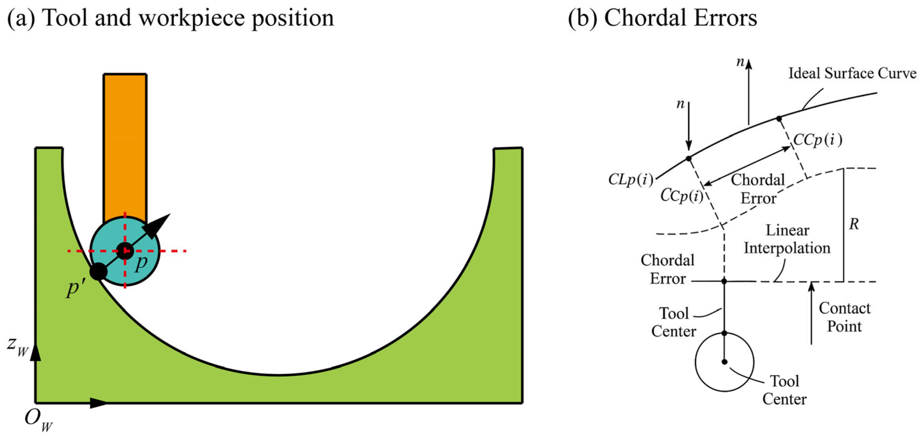
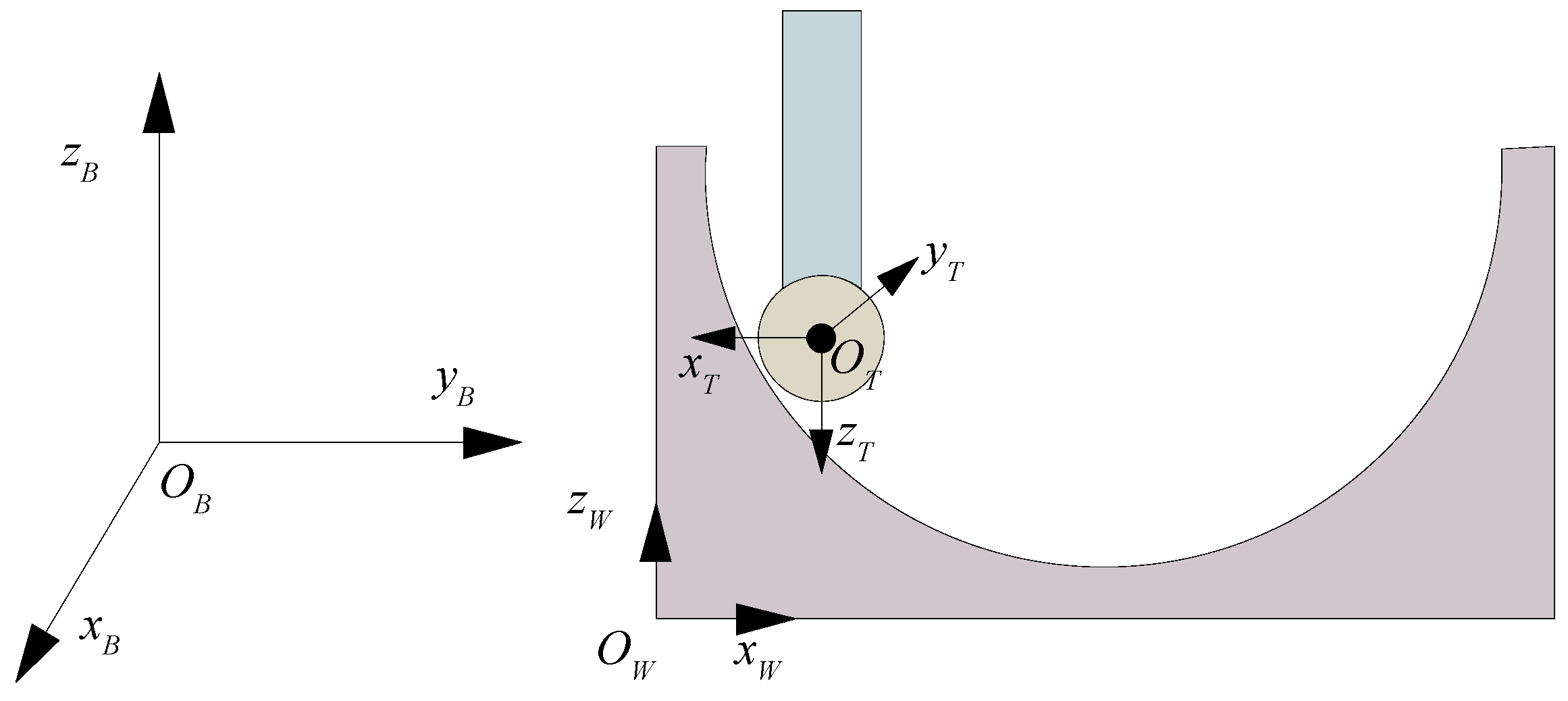
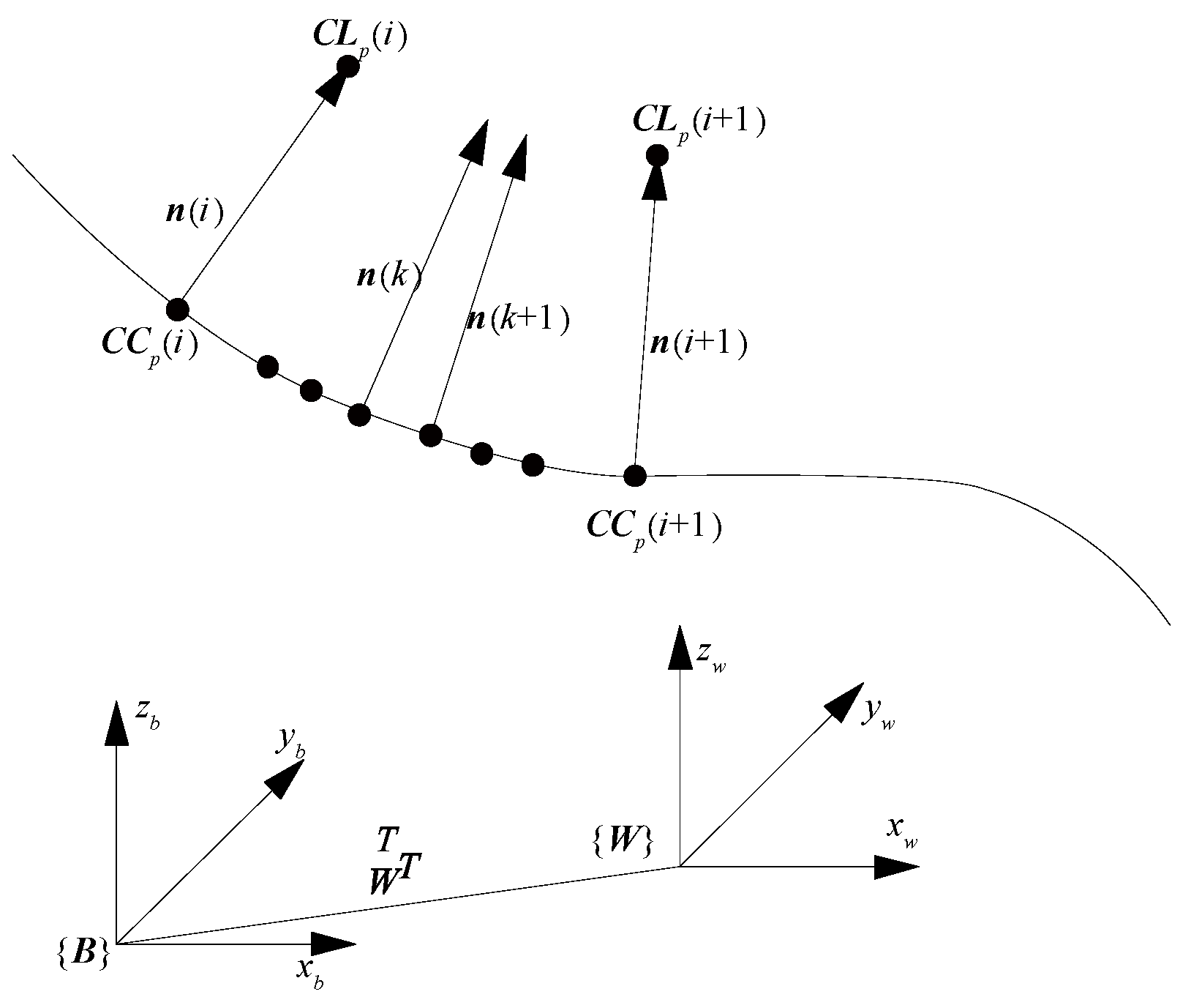
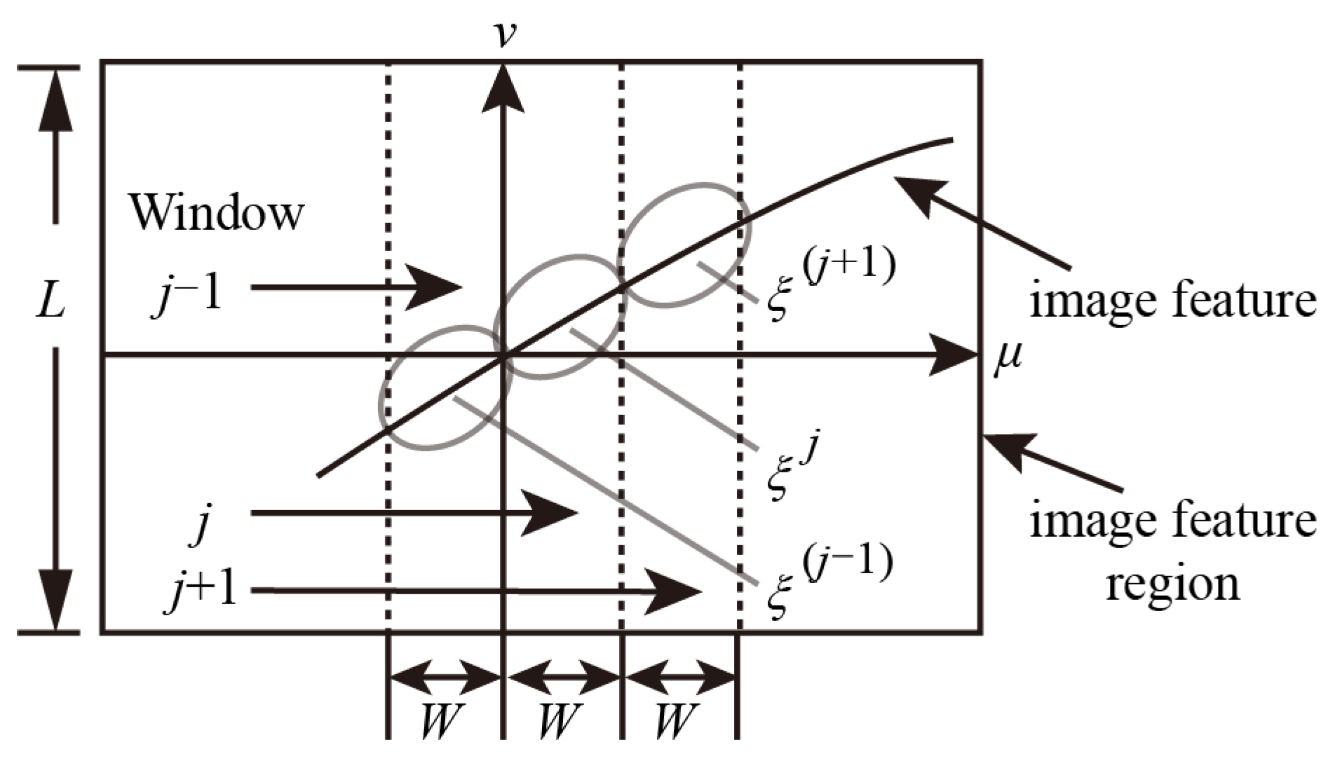
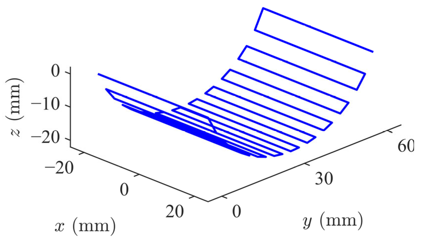
2.1. Generation of the Toolpath

This study investigates a small concave surface product polished using a spherical tool. As illustrated in Figure 1a, point p represents the tool center’s position in the workpiece coordinate system, while vector n denotes the surface normal at the polishing point. The cutter location point coincides with p, yielding the matrix expression C = [P n]. To optimize tool path generation, we first determine the positions and normal vectors (p′) of polishing points using a custom trajectory generator developed in UG software (NX 2019) [33]. Subsequently, the tool center trajectory is calculated by adjusting the polishing point trajectory according to the tool’s geometry.

Figure 1b presents a schematic diagram of tool compensation incorporating critical geometric considerations for precision polishing. The diagram delineates four key factors influencing polishing accuracy: (1) the spatial relationship between cutter location points (CLPs) and contact points (CCPs); (2) the surface normal vectors at contact points; (3) radius-based tool compensation; and (4) chordal errors resulting from linear interpolation between adjacent tool contact points on curved surfaces.

Chordal errors represent the deviation between the actual curved surface and the linear approximation used during tool path planning. These errors are particularly significant when polishing complex curved surfaces, as they directly impact surface finish quality. The magnitude of chordal errors depends on both the curvature of the workpiece surface and the density of interpolation points. Higher curvature regions and wider spacing between interpolation points result in larger chordal errors, necessitating adaptive control strategies to maintain consistent polishing quality.

The curved workpiece is affixed with the workpiece coordinate system, denoted as O_W-x_Wy_Wz_W [34]. Location of the polished point p₀ in the coordinates of the workpiece {W} is assumed to be ^WP_p′, and the normal vector at p₀ is defined as ^Wn_p′ = [cos^Wα_p′ cos^Wβ_p′ cos^Wγ_p′]. To calculate the surface area of a spherical polishing tool (denoted as p), move the point p′ by a distance equal to the radius R of the sphere along the normal vector. The location of p in the work coordinate system {W} is computed using the translation matrix.

$$\begin{array}{c}\left[\begin{array}{c}{}^{Q}P_{p_w}\\ 1\end{array}\right]=\left[\begin{array}{c}{}^{Q}x_{p_w}\\ {}^{Q}y_{p_w}\\ {}^{Q}z_{p_w}\\ 1\end{array}\right]=\\ \left[\begin{array}{cccc}1& 0& 0& R_w\cos {}^Q\alpha _{p_0}\\ 0& 1& 0& R_w\cos {}^Q\beta _{p_0}\\ 0& 0& 1& R_w\cos {}^Q\gamma _{p_0}\\ 0& 0& 0& 1\end{array}\right]\left[\begin{array}{c}{}^{Q}x_{p_0}\\ {}^{Q}y_{p_0}\\ {}^{Q}z_{p_0}\\ 1\end{array}\right]\end{array}$$

(1)

The surface norm vector expression for this point is as follows:

$${}^W\mathit{n}_p={}^W\mathit{n}_{p^{\prime }}$$

(2)

The transformation matrix based on the workpiece coordinate {W} and the basic robot coordinate {B}, a positional expression for the basic coordinates {B} of a polished tool’s multi-axis cutter, denoted as ${}_W{}^B\mathit{T}$, can be derived:

$$\left[\begin{array}{cc}{}^B\mathit{P}_p& {}^B\mathit{n}_p\\ 1& 0\end{array}\right]={}_W{}^B\mathit{T}\left[\begin{array}{cc}{}^W\mathit{P}_p& {}^W\mathit{n}_p\\ 1& 0\end{array}\right]$$

(3)

As shown in Figure 2, interaction of the polishing tool with the concave workpiece during machining is prevented by maintaining a constant orientation of the polishing tool coordinate {OT} with regard to the reference coordinate {OB}. Assume that in the base coordinates {OB}, the Z_B-axis direction vector is [0 0 1]^T. Simultaneously, in the tool coordinate {O_T}, the Z_T-axis direction vector is specified as [0 0 −1]^T throughout the process. This specification implies that the rotation matrix R, which connects these two coordinate systems, remains constant. The constant rotation matrix R corresponds to specific Roll-Pitch-Yaw (RPY) angles that can be computed as ${}^{B}O_T={\left[\begin{array}{ccc}{}^B\varphi _T& {}^B\theta _T& {}^B\phi _T\end{array}\right]}^T$. Similarly, the location of the origin of the tool coordinate system in the base corresponds to the position of the tool’s sphere center, represented by ${}^{B}P_{O_T}$. The trajectory of the tool in Cartesian space throughout the process can be expressed as a 6 × 1 vector, composed of ${}^{B}P_{O_T}$ and ${}^{B}O_T$:

$${}^{B}X_E={\left[\begin{array}{cc}{}^{B}P_{O_E}^T& {}^{B}O_E^T\end{array}\right]}^T$$

(4)

In this study, the offline trajectory planning for the mold surface is achieved through the use of UG software (NX 2019) platform secondary development technology. A series of offline multi-axis tool positions is obtained, and these positions can be expressed as:

$$CL(i)={[C{L}_p^{\mathit{T}}(i),C{L}_o^{\mathit{T}}(i)]}^{\mathit{T}},i=1,2\cdots ,m$$

(5)

The center position of tool is expressed as $C{L}_p^{\mathit{T}}(i)={\left[C{L}_x(i),C{L}_y(i),C{L}_z(i)\right]}^{\mathit{T}}$, The contact normal vector between the tool and the workpiece surface is denoted by $C{L}_o^{\mathit{T}}(i)={[C{L}_o(i),C{L}_o(i),C{L}_o(i)]}^{\mathit{T}}$, m is the number of polishing points.

When utilizing a spherical tool, the determination of the cutter position involves offsetting the cutter contact point along the normal vector by the radius of the tool. Subsequently, the tool position in the workpiece coordinate system is converted to the robot coordinate system:

$$\left\{\begin{array}{l}{}^B\mathit{CL}_p^T(i)={\displaystyle \frac{B}{W}}T{}^W\mathit{CC}_p^T(i)+{}^B\mathit{CL}_o(i)R\hfill \\ {}^B\mathit{CL}_o^T(i)={\displaystyle \frac{B}{W}}T{}^W\mathit{CC}_o^T(i)\hfill \end{array}\right.$$

(6)

The position of the tool contact point in the workpiece coordinate system is represented by ${}^W\mathit{CC}_p^T(i)$, and the normal vector is represented by ${}^W\mathit{CC}_o^T(i)$, where R is the radius of the tool.

In the actual polishing process, even when adjacent polishing points meet the accuracy requirements, linear interpolation is necessary for these points. This requirement arises from the limitations set by the interpolation cycle and the maximum velocity in the control process by the upper computer. This can be expressed as:

$$D(i)=CL(i+1)-CL(i)=[D_p^T(i),D_o^T(i)]$$

(7)

where $D_p^T(i)$ and $D_o^T(i)$ is the increments in position and normal vectors, respectively.

The expression for the actual position of the polishing tool contact point can be formulated when the desired interpolation speed of adjacent polishing points is represented as v(k):

$$x_d(k)=x_d(k-1)+v(k)\Delta t(k=1,2,\dots ,n)$$

(8)

where Δt is the interpolation period, n is the actual number of polishing points after interpolation.

The formula for interpolating the normal vector can be expressed when the normal vectors of adjacent polishing points are represented as n(i) and n(i + 1):

$$n(k)=n(i)+[n(i+1)-n(i)]{\displaystyle \frac{‖x_d(k)-C{L}_p^{\mathit{T}}(i)‖}{‖D_p(i)‖}}$$

(9)

The schematic diagram of normal vector interpolation is shown in Figure 3 [35].

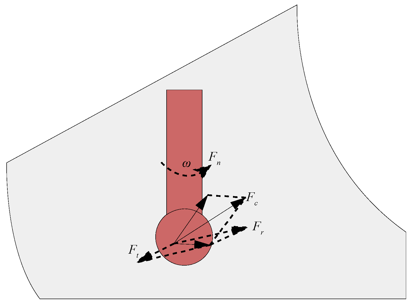
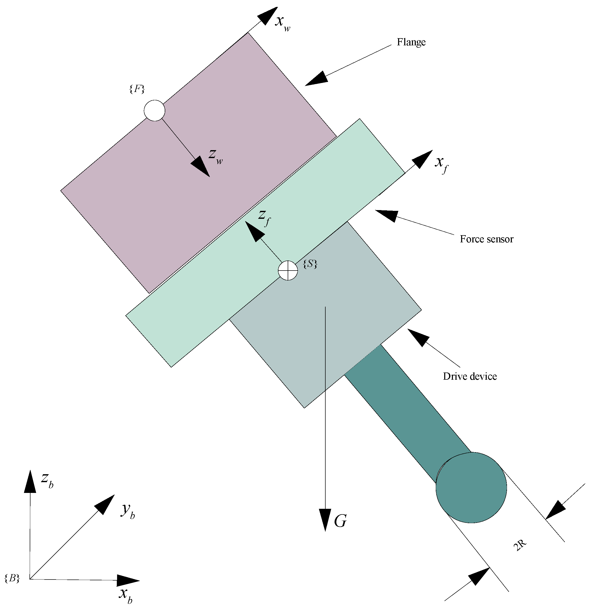
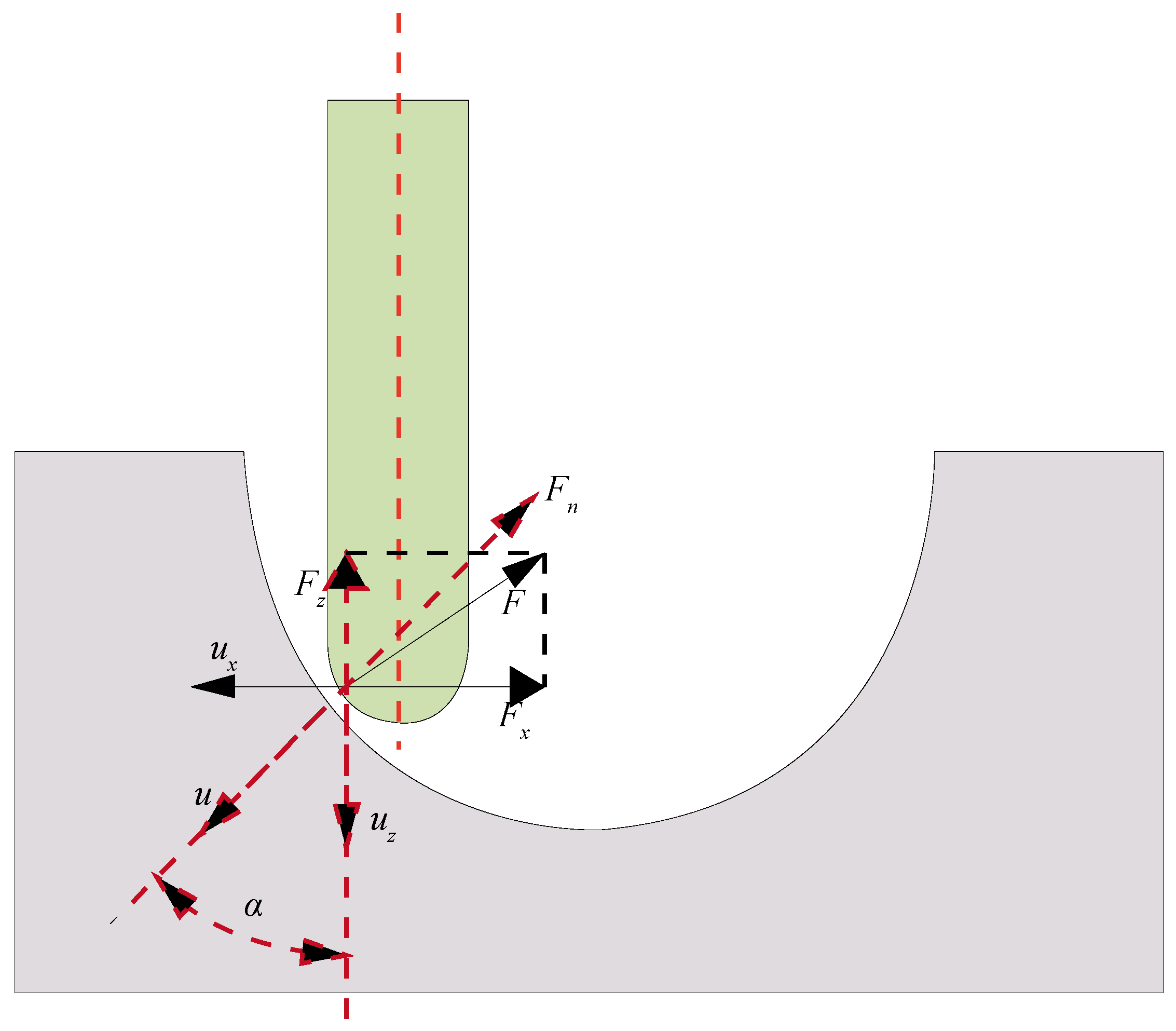
2.2. Force Analysis and Compensation

In this study, a spherical polishing tool is employed and maintained perpendicular to the horizontal plane throughout the polishing process. The contact force between the workpiece and the polishing tool is measured using the ME3DT120 three-axis force sensor. As illustrated in Figure 4, the force is exerted on the polishing tool by the workpiece surface.

The force exerted by the polishing tool on the workpiece is denoted as F_c, which comprises three components: F_t, F_r, and F_n. F_t represents the frictional force acting opposite to the feed direction, F_n corresponds to the normal reaction force exerted by the surface perpendicular to the tool’s orientation, and F signifies the frictional force generated by the tool’s high-speed rotation:

$$F_c=F_t+F_r+F_n$$

(10)

When polishing a surface, the force exerted by the polishing tool (${}^{s}F_c$) can be measured. A force transducer is mounted between the robot end-effector and the polishing tool for this purpose. The measured resultant force (${}^{s}F_m$) during processing mainly comprises three components: the force exerted by the component on the polishing tool (${}^{s}F_c$), the gravitational force of the polishing tool itself (${}^{s}F_G$), and the inertial force (${}^{s}F_I$).

$${}^{s}F_m={}^{s}F_c+{}^{s}F_G+{}^{s}F_I$$

(11)

$${}^{s}F_m=\sqrt{{\left|F_x\right|}^2+{\left|F_y\right|}^2+{\left|F_z\right|}^2}$$

(12)

The force components along three sensor directions are denoted as F_x, F_y, and F_z. The force components along three sensor directions are denoted as F_x, F_y, and F_z. The inertia force of the polishing tool concerning the contact force with the workpiece and gravity acting on the tool can be ignored due to the short step distances between neighboring machining points and the small acceleration. Thus, the inertia force can be ignored. As a result, Equation (11) can be expressed as:

$${}^{s}F_m={}^{s}F_c+{}^{s}F_G$$

(13)

During the polishing procedure, the measurement of the force used for polishing ${}^{s}F_c$ is significantly affected by the gravity acting on the polishing tool and therefore needs to be compensated. In Figure 5, the rotation angles α, β and γ of the wrist coordinate system of the robot with respect to the base coordinate are depicted. Therefore, the transformation of the attitude of the wrist coordinate concerning the base coordinate can be described as follows:

$$\begin{array}{c}{}_F{}^{B}R_{\mathit{zyx}}=Rot(z,\alpha )Rot(y,\beta )Rot(x,\gamma )=\\ \left[\begin{array}{ccc}c\alpha c\beta & c\alpha s\beta s\gamma -s\alpha c\gamma & c\alpha s\beta c\gamma +s\alpha s\gamma \\ s\alpha c\beta & s\alpha s\beta s\gamma +c\alpha c\gamma & s\alpha s\beta c\gamma -c\alpha s\gamma \\ -s\beta & c\beta s\gamma & c\beta c\gamma \end{array}\right]\end{array}$$

(14)

where c = cos, s = sin.

The attitude transformation of the force sensor concerning the wrist coordinate system is:

$${}_S{}^{B}R_{\mathit{zx}}=\left(\begin{array}{ccc}1& 0& 0\\ 0& -1& 0\\ 0& 0& -1\end{array}\right)$$

(15)

The attitude transformation of the force sensor concerning the base coordinate can be derived from Equations (14) and (15):

$${}_S{}^{B}R={}_F{}^{B}R_{\mathit{zx}}^{F}R_{\mathit{zx}}$$

(16)

The actual normal polishing force can be obtained from Equations (13) and (16):

$${}^{B}F_n(k)={}^{B}F_c·{}^{B}n(k)={}_S{}^{B}R({}^{S}F_m-{}^{S}F_G)·{}^{B}n(k)$$

(17)

where ${}^{B}n(k)$ is the normal vector of the fundamental coordinate.

To maintain the accuracy of collected data and avoid interference, it is crucial to keep the cutting tool’s axis consistently in a vertical downward position. This ensures stable sensor data despite changes in the direction of the cutting tool’s axis. In this study, ${}^{S}F_G={[0,0,-G]}^T$, G represents the magnitude of gravity acting on the front-end device.

3. Control Design for Polishing Robotic Systems

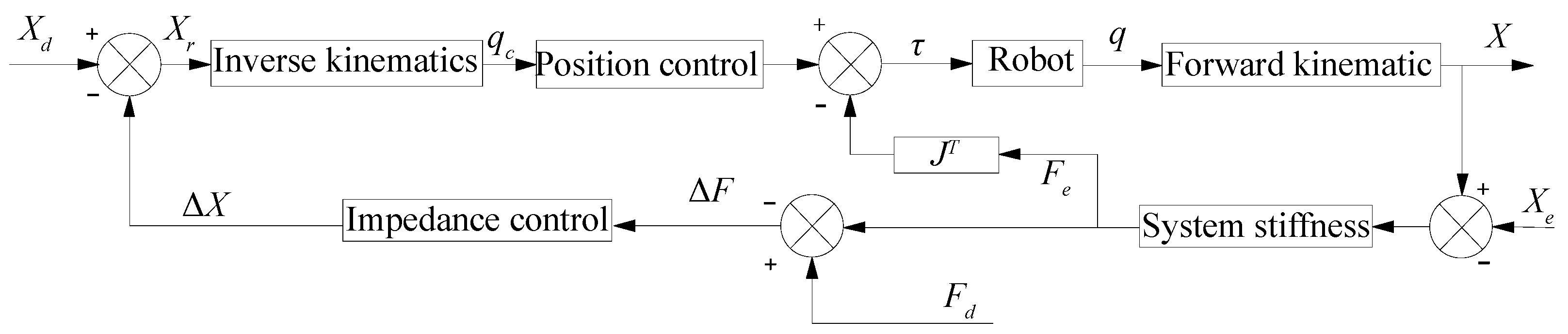
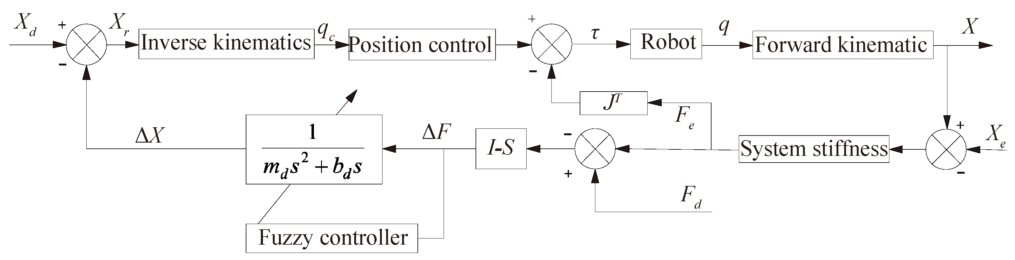
3.1. Impedance Control

Maintaining a consistent relative velocity between the polishing tool and the workpiece surface is crucial. The surface quality of the workpiece depends on the contact force between them. Unstable contact force may lead to uneven material removal from the workpiece surface. Therefore, the robot must achieve precise position tracking and maintain stable force throughout the polishing process to ensure surface uniformity. Position-based impedance control, a widely adopted method for force control in end-effector polishing, converts dynamic force errors into position errors without relying on accurate dynamic models [36].

Position-based impedance control is illustrated in Figure 6. Sensors integrated into the robot system measure the force and displacement between the end-effector tool and the workpiece surface. The collected data is transmitted to the controller, which computes the necessary force and displacement commands. These commands are then sent to the robot’s actuator, guiding the motion of the end-effector tool. By adjusting force and displacement commands, the controller achieves the desired polishing force and position tracking. To ensure stability and precision, force and displacement sensors provide continuous feedback to the control system. Force sensors measure the magnitude and direction of contact forces, while displacement sensors monitor the relative movement of the end-effector tool with respect to the workpiece surface. Position-based impedance control enables precise force regulation during polishing, ensuring surface uniformity. This control method is essential in automated polishing and surface treatment applications, improving product quality and production efficiency.

The desired reference trajectory for the force is denoted as X_d, while the desired force is represented by F_d. The relationship of the force error ΔF and location compensation ΔX can be expressed as [37]:

$$\mathit{M}\Delta \ddot{\mathit{X}}+\mathit{B}\Delta \dot{\mathit{X}}+\mathit{K}\Delta \mathit{X}=\Delta \mathit{F}$$

(18)

where M, B, K is the matrix for mass coefficient, matrix for damping coefficient, and matrix for stiffness coefficient, respectively.

The steady-state error analysis accounts for the interdependence between force and position control. To mitigate interference with trajectory tracking while clearly decoupling position control from force control, impedance control is selectively implemented solely along the surface normal direction. Based on the control block diagram, the following expression can be derived [38]:

$$\left\{\begin{array}{l}\Delta f=f_d-f_s=m_d\ddot{e}+b_d\dot{e}+ke\hfill \\ f_s=k_{s}e=k_s(x_c-x_e)\hfill \\ x_c=x_d-e\hfill \end{array}\right.$$

(19)

where f_d is the desired force in the normal direction, k_e is the stiffness of the end effector in the normal direction, x_e is the position of end actuator, e is the position error of polishing.

Therefore, the following can be obtained:

$$\Delta f=f_d+k_e{x}_e-k_e(x_d-e)$$

(20)

Applying the Laplace transform to Equations (19) and (20), the following can be obtained:

$$\begin{array}{c}\Delta f(s)(m_d{s}^2+b_{d}s+k_d-k_e)=\\ (m_d{s}^2+b_{d}s+k_{d}s)\left[f_d+k_e(x_e-x_d)\right]\end{array}$$

(21)

When the system is stabilized, the force tracking error is:

$$\Delta f_{ss}={\displaystyle \frac{k_d}{k_d-k_e}}(f_d+k_e(x_e-x_d))$$

(22)

If ∆f_ss = 0, then:

$$k_d=0$$

(23)

Or:

$$x_d=x_e+{\displaystyle \frac{f_d}{k_e}}$$

(24)

According to Equation (22), the system’s tracking error vanishes only if either Equation (23) or Equation (24) is satisfied. However, in practical polishing applications, the stiffness of the robotic end-effector varies dynamically, complicating its precise measurement [39]. To address this, the stiffness gain k_d is set to zero in this study, ensuring that any system stiffness k_e satisfies the steady-state requirements. Consequently, the impedance control law in Equation (19) can be reformulated as follows:

$$\Delta f=f_d-f_e=m_d\ddot{e}+b_d\dot{e}$$

(25)

Let $x=v_n=\dot{e}$, the following can be obtained:

$$\dot{x}=-{\displaystyle \frac{b_d}{m_d}}x+{\displaystyle \frac{\Delta f}{m_d}}$$

(26)

By solving Equation (26), the following can be obtained:

$$x(t)=e^{-{\displaystyle \frac{b_d}{m_d}}t}x(0)+{\displaystyle {\int }_0^t{e}^{-\frac{b_d}{m_d}(t-\tau )}}{\displaystyle \frac{\Delta f}{m_d}}d\tau$$

(27)

Assuming that m_d and b_d are constants within the sampling time ∆t, x(k) can be obtained as the discrete value of x(t) at t = k∆t by solving Equation (27):

$$v_n(k)=e^{-{\displaystyle \frac{b_d}{m_d}}\Delta t}{v}_n(k-1)-{\displaystyle \frac{e^{\frac{b_d}{m_d}}-1}{b_d}}(f_d-f_e(k))$$

(28)

The control law of the normal polishing force and the normal velocity can be derived, and the normal displacement compensation can be calculated:

$$\Delta x(k)={\nu }_n(k)\Delta t$$

(29)

3.2. Fuzzy Adaptive Impedance Control

In the field of robotic automatic polishing, control algorithms based on fixed stiffness are widely employed. However, such designs possess inherent limitations, as they often fail to adequately adapt to diverse operational conditions encountered during polishing, including variations in workpiece geometry, dimensions, and material properties. Moreover, since stiffness selection directly influences polishing force and velocity, fixed stiffness designs typically cannot achieve optimal polishing outcomes. In contrast, variable stiffness control systems offer substantial advantages by dynamically adjusting stiffness according to real-time operational conditions, thereby improving process adaptability and polishing quality. These systems also enhance robotic flexibility, enabling the handling of more complex polishing tasks. Nevertheless, implementing variable stiffness control presents significant challenges, requiring high-speed, high-precision control systems capable of processing substantial data volumes and executing complex real-time adjustment algorithms. Additionally, such designs must account for robotic dynamic performance characteristics, including response speed and stability, inevitably increasing system complexity.

The polishing system in this study comprises a robotic arm, a front-end unit, and a cutting tool. During the polishing process, the overall system stiffness is determined by three factors: the robotic arm’s structural rigidity, the front-end device’s compliance, and the cutting tool material’s elasticity. Given that the robotic arm exhibits significantly higher stiffness than other components, the analysis primarily focuses on how the front-end device and cutting tool material influence polishing forces. Consequently, the system stiffness can be effectively modeled as:

$$k={\displaystyle \frac{k_s{k}_g}{k_s+k_g}}$$

(30)

where k_s and k_g is the stiffness of the front-end device and the cutting tool material, respectively.

As shown in Figure 7, the system stiffnesses of the polishing system in both the horizontal and vertical directions are assumed to be k_x and k_z, respectively, the displacement compensation along the normal direction is u, the displacement deformations in the horizontal and vertical directions as well as the forces generated by the displacements are u_x, k_z, F_x, and F_z, respectively. The angle α represents the inclination between the surface normal and the tool axis, and the unit normal to surface vectors is n. The displacement compensation along the normal direction is u, and the forces generated by the displacements in the horizontal and vertical directions are n, respectively:

$$F=[F_x,F_z]=[-k_x{u}_x,-k_z{u}_z]$$

(31)

$$n=[-{\displaystyle \frac{u_x}{\sqrt{{u_x}^2+{u_z}^2}}},-{\displaystyle \frac{u_z}{\sqrt{{u_x}^2+{u_z}^2}}}]$$

(32)

$$F_n=F·n$$

(33)

$$\left\{\begin{array}{l}{k}_e={\displaystyle \frac{F_n}{u}}={\displaystyle \frac{k_x{u_x}^2+k_z{u_z}^2}{u_x^2+{u_z}^2}}\hfill \\ \alpha =\arctan ({\displaystyle \frac{u_x}{u_z}})\hfill \end{array}\right.$$

(34)

When k_x = k_z, it follows that F_n = F and k_e = k_x = k_z. In this case, the normal-system stiffness depends both on the orientations of the surface normal vectors and on the stiffnesses of the horizontal and vertical subsystems, which are conveniently characterized by the directly measurable parameters k_x and k_z.

To accurately characterize the relationship between normal force and displacement, the tool axis was aligned vertically downward and computer-controlled to approach the workpiece along the surface normal at a constant slow rate. During each control cycle, the tool advanced by 0.05 mm; if the measured normal force exceeded 30 N, the tool was retracted. To assess the influence of the angle α on system stiffness, tests were performed at 45° and 60° using a spherical rubber polishing tool. Figure 8 presents the force–displacement curves, where a normal force of zero denotes no contact. Curve fitting yields effective stiffness values of k_e = 37.366 N/mm at α = 45° and 35.149 N/mm at α = 60°, indicating that the system’s normal stiffness varies with α.

In fact, variations in the normal vector, normal polishing force at different polishing points, desired force, and tool material properties collectively influence the normal system stiffness during the polishing process. In practical control applications, when the detected force error is Δf, the desired displacement is adjusted inversely proportional to the system stiffness: a smaller adjustment is made when the stiffness is high, while a larger adjustment compensates for the error when the stiffness is low. Since a single impedance control strategy cannot adequately meet practical control requirements, this study employs a fuzzy adaptive impedance control approach. This strategy dynamically adjusts the impedance model parameters based on real-time force error feedback, thereby indirectly adapting to the system stiffness. The underlying principle of this method is as follows: when the force error and its rate of change are large, the mass coefficient m_d is increased and the damping coefficient b_d is decreased to enhance the control system’s response speed. Conversely, when the force error and its rate are small, m_d is reduced and b_d is increased to minimize system overshoot. To simplify the system dynamics and reduce complexity, this study focuses solely on adjusting the damping coefficient b_d, as the quality factor’s sensitivity to dynamic responses is less critical. Figure 9 illustrates the schematic of fuzzy adaptive impedance control, where S and I-S represent the position control space and force control space, respectively.

The input linguistic variables are force deviation e and force deviation rate ec, while the output linguistic variable is ∆b. The basic domains are [−X_e, X_e] and [−X_ec, X_ec, −Y_b, Y_b], respectively. The fuzzy sets of language variables for input and output are created by triangular affiliation functions with {NB, NM, NS, ZE, PS, PM, PB}, increasing from NB to PB. The input quantization factors are G_e and G_ec. Therefore, the transformation relationship from the basic domain to the fuzzy domain is as follows:

$$\left\{\begin{array}{c}{X_e}^{\ast }={\displaystyle \frac{X_e}{G_e}}\\ {X_{ec}}^{\ast }={\displaystyle \frac{X_{ec}}{G_{ec}}}\end{array}\right.$$

(35)

The fuzzy control rules governing the adjustment of the damping coefficient are presented in

Table 1. The rules of fuzzy adaptive impedance control.

${∆b}^{\mathit{*}}$		ec
		NB	NM	NS	ZE	PS	PM	PB
e	NB	PB	PM	PS	ZE	ZE	ZE	ZE
	NM	PB	PM	PS	ZE	ZE	ZE	NS
	NS	PB	PS	PS	ZE	ZE	NS	NM
	ZE	PB	PS	PS	ZE	NS	NB	NB
	PS	PM	PS	ZE	ZE	NS	NM	NB
	PM	PS	ZE	ZE	ZE	NS	NM	NB
	PB	ZE	ZE	ZE	ZE	NS	NM	NB

[40].

A parallel processing architecture is implemented for fuzzy inference, while the center-of-gravity method is adopted for defuzzification:

$$\Delta b^{\ast }={\displaystyle \frac{{\displaystyle \sum _{i=1}^n}{\mu }_{i}R(e,ec)}{{\displaystyle \sum _{i=1}^n}R(e,ec)}}$$

(36)

where μ_i is the i-th fuzzy output. R(e, ec) is the fuzzy output obtained from the fuzzy rule.

The exact solution can be obtained by setting the output quantization factor to G_b:

$$\Delta b=G_b\Delta b^{\ast }$$

(37)

Therefore, the actual damping parameter is:

$$b_d^{\prime }=b_d+\Delta b$$

(38)

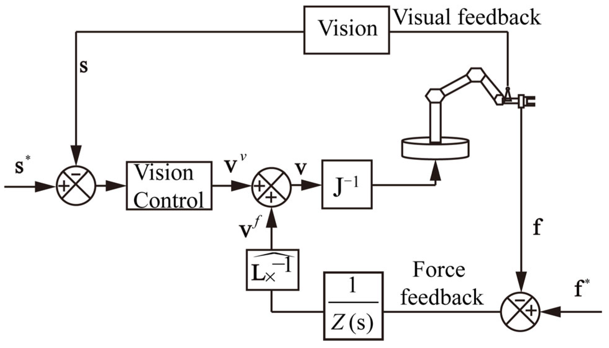
3.3. Vision-Guided Fuzzy Adaptive Impedance Control

When a complete interaction matrix is established via visual feedback, the system can perform high-precision positioning tasks [41]. However, vision-only control is vulnerable to ambient-lighting variations and occlusions, which degrade performance. Conversely, position–force control schemes require accurate geometric models of the environment for path planning. To overcome these limitations, this chapter proposes a hybrid visual–force control method. First, an SVR-Jacobian estimator models the mapping between image-feature tracking paths and the robot’s joint angles. Then, under constrained conditions, an adaptive impedance controller regulates the normal force. By fusing vision and force feedback in this way, the approach enhances control-loop stability and reduces dependence on exact environmental models.

3.3.1. Description of the Impedance Vision-Force Control Approach

As depicted in Figure 10, the resultant control vector within the vision-force impedance control system is formulated as $v=v^v+v^f$, where the kinematic screw $v^v$ is derived from the vision control law, and the force control loop determines $v^f$. By focusing solely on the stiffness matrix within the impedance control law and employing a standard visual servo methodology, the formulation for the impedance vision-force control can be articulated as follows [42,43]:

$$v=-\lambda \widehat{L^{+}}(s-s^{\ast })+{\widehat{L_{\times }}}^{-1}{K}^{-1}(f-f^{\ast })$$

(39)

where $\widehat{L_{\times }}$ relates $v$ and $\dot{\mathit{x}}$ according to $\dot{x}=\widehat{L_{\times }}·v$.

In a serial control architecture, the actual kinematic screw s may deviate from the desired screw s* and the measured force f may differ from the target force f*, even when the end-effector velocity v is zero. Such discrepancies can trap the controller in a local minimum, provoking oscillatory responses. Consequently, conventional vision–force control schemes often fall short of the precision demanded by polishing processes with time-varying stiffness.

3.3.2. SVR-Based Jacobi Mapping Method

The performance of a visual-servo system depends critically on the choice of image features used within its control loop. In image-based visual servoing, careful selection and extraction of these features is essential, as they directly affect control-law stability, algorithmic robustness, and, ultimately, overall system accuracy.

To achieve precise six-degree-of-freedom positioning in three-dimensional space, the visual-servo control system employs six unique sets of visual markers, with each set dedicated to monitoring the motion of a specific robot joint. As depicted in Figure 11, the image features ${\xi }^{(j)}={[{\xi }_1^{(j)},{\xi }_2^{(j)},\cdots {\xi }_6^{(j)}]}^T$ selected for utilization are delineated by a window indexed as j, wherein the dimensions of the window are characterized by its length L and width W.

The centroid coordinates of each independent visual feature ${\xi }^{(j)}$ can then be computed as follows:

$$\begin{array}{l}{\xi }_1^{(j)}={\displaystyle \frac{{\displaystyle \sum _{q=1}^L}{\displaystyle \sum _{r=1}^W}{g}_{qr}^{(j)}·q}{{\displaystyle \sum _{q=1}^L}{\displaystyle \sum _{r=1}^W}{g}_{qr}^{(j)}}}\hfill \\ {\xi }_2^{(j)}={\displaystyle \frac{{\displaystyle \sum _{q=1}^L}{\displaystyle \sum _{r=1}^W}{g}_{qr}^{(j)}·r}{{\displaystyle \sum _{q=1}^L}{\displaystyle \sum _{r=1}^W}{g}_{qr}^{(j)}}}\hfill \\ {\xi }_3^{(j)}={\displaystyle \sum _{q=1}^L}{\displaystyle \sum _{r=1}^W}{g}_{qr}^{(j)}\hfill \end{array}$$

(40)

where $g_{qr}^{(j)}=\left\{\begin{array}{c}0\left(\mathrm{white}\mathrm{pixels}\right)\\ 1\left(\mathrm{black}\mathrm{pixels}\right)\end{array}\right.$

The principal and secondary axes of the corresponding ellipse are:

$$\begin{array}{l}{\xi }_4^{(j)}={\displaystyle \frac{{\lambda }_{20}^{(j)}+{\lambda }_{02}^{(j)}+\sqrt{{\left({\lambda }_{20}^{(j)}-{\lambda }_{02}^{(j)}\right)}^2+4{\left({\lambda }_{11}^{(j)}\right)}^2}}{2{\xi }_3^{(j)}}}\hfill \\ {\xi }_5^{(j)}={\displaystyle \frac{{\lambda }_{20}^{(j)}+{\lambda }_{02}^{(j)}-\sqrt{{({\lambda }_{20}^{(j)}-{\lambda }_{02}^{(j)})}^2+4{({\lambda }_{11}^{(j)})}^2}}{2{\xi }_3^{(j)}}}\hfill \end{array}$$

(41)

The direction is:

$${\xi }_6^{(j)}={\displaystyle \frac{1}{2}}{\tan }^{-1}{\displaystyle \frac{{\lambda }_{11}^{(j)}}{{\lambda }_{20}^{(j)}-{\lambda }_{02}^{(j)}}}$$

(42)

where ${\lambda }_{11}^{(j)}={\displaystyle \sum _{q=1}^L}{\displaystyle \sum _{r=1}^W}{g}_{qr}^{(j)}·[q-{\xi }_1^{(j)}][r-{\xi }_2^{(j)}]$, ${\lambda }_{02}^{(j)}={\displaystyle \sum _{q=1}^L}{\displaystyle \sum _{r=1}^W}{g}_{qr}^{(j)}·{[q-{\xi }_1^{(j)}]}^2$, ${\lambda }_{02}^{(j)}={\displaystyle \sum _{q=1}^L}{\displaystyle \sum _{r=1}^W}{g}_{qr}^{(j)}·{[r-{\xi }_2^{(j)}]}^2$

In numerous contexts, the relationship between a robot’s six-degree-of-freedom joint position parameters $\theta ={[{\theta }_1,{\theta }_2,\cdots {\theta }_6]}^T$ and visual feature data exhibits complex nonlinear dynamics. To model this relationship, this study employs a mathematical formulation based on support vector regression (SVR). Typically, SVR modeling involves a nonlinear transformation that maps multiple input variables to a single output. However, for the relationship between robotic joint angles and image feature vectors, separate SVR models must be constructed for each independent element of the feature vector due to the system’s inherent multi-input, multi-output nature. When developing a least squares support vector regression (LS-SVR) model, the first step is to map and transform the original dataset into a higher-dimensional feature space $\psi (x)=[\phi (x_1),\phi (x_2),\cdots ,\phi (x_n)]$. Within this space, an optimized linear regression model is constructed to achieve accurate predictions of the input data.

$$f(x)={\displaystyle \sum _{i=1}^n}{\omega }_i{\phi }_i(x)+b$$

(43)

The framework of the model integrates a nonlinear transformation function, denoted as φ(·), in conjunction with a weight matrix ω and a bias term B. The objective function is derived by addressing the below optimization challenge:

$$\begin{array}{l}\min J(\omega ,\xi )={\displaystyle \frac{1}{2}}{\omega }^T\omega +{\displaystyle \frac{1}{2}}\gamma {\displaystyle \sum _{i=1}^n}{\xi }_i^2\hfill \\ \mathrm{s}.t\mathrm{.}{y}_i={\omega }^T\phi (x_i)+b+{\xi }_i,i=1,2,\cdots ,n\hfill \end{array}$$

(44)

The variable ${\xi }_i$ is used to represent the error term, while the regularization penalty factor is symbolized by γ. In addressing the optimization problem, the method of Lagrange multipliers is invoked, which involves formulating a Lagrange function.

$$L(\omega ,b,\xi ,\alpha )=J(\omega ,\xi )-{\displaystyle \sum _{i=1}^n}{\alpha }_i{\omega }^T\phi (x_i)+b+{\xi }_i-y_i$$

(45)

where α_i is the Lagrange multiplier.

The optimality conditions can be derived using the KKT (Karush-Kuhn-Tucker) theorem:

$${\displaystyle \frac{\partial L}{\partial \omega }}=0,{\displaystyle \frac{\partial L}{\partial b}}=0,{\displaystyle \frac{\partial L}{\partial {\xi }_i}}=0,{\displaystyle \frac{\partial L}{\partial {\alpha }_i}}=0$$

(46)

Hence, the following derivation can be established:

$$\omega ={\displaystyle \sum _{i=1}^n}{\alpha }_i\phi (x_i),{\displaystyle \sum _{i=1}^n}{\alpha }_i=0,{\alpha }_i=\gamma {\xi }_i,{\omega }^T\phi (x_i)+b+{\xi }_i-y_i=0$$

(47)

When a sequence of iterations is performed on variable i from 1 to n, the following conclusions can be derived:

$$\left[\begin{array}{cc}0& I^T\\ I& \Omega +{\displaystyle \frac{1}{\gamma }}\end{array}\right]\left[\begin{array}{c}b\\ \alpha \end{array}\right]=\left[\begin{array}{c}0\\ y\end{array}\right]$$

(48)

where $y=[y_1,y_2,\cdots y_n]$, $I={[1,1,\cdots 1]}^{\mathit{T}}$, $\alpha ={[{\alpha }_1,{\alpha }_2,\cdots {\alpha }_n]}^{\mathit{T}}$, ${\mathsf{\Omega }}_{ij}=\phi (x_i)\phi (x_j)$

The parameters α and b are estimated via a least-squares procedure as specified in Equation (48). Thereafter, the resulting predictive function can be expressed explicitly as follows:

$$f(x)={\displaystyle \sum _{i=1}^n}{\alpha }_{i}K(x,x_i)+b$$

(49)

where the kernel function is denoted by K(x, x_i),

After accurately identifying image features, an LS-SVR network model was constructed for a specific visual servo task. The model learns the direct mapping between the tracked image feature trajectories and robot joint positions through supervised training. Specifically, the relationship between the robot joint angles and the feature dimension ${\xi }_k^{(j)}(k=1,2,\cdots 6)$ can be explained by the following expression:

$${\xi }_k^{(j)}(\theta )={\displaystyle \sum _{i=1}^n}{\alpha }_{ki}K(\theta ,{\theta }_i)+b_k$$

(50)

In this study, the Gaussian kernel is selected as the kernel function:

$${\xi }_k^{(j)}(\theta )={\displaystyle \sum _{i=1}^n}{\alpha }_{ki}\exp (-\theta -{{\theta }_i}^2/2{\sigma }^2)+b_k$$

(51)

Each element of the Jacobian matrix is obtained by differentiating an individual joint angle, thereby directly quantifying how variations in each joint’s angle affect the corresponding kinematic feature:

$$\left\{\begin{array}{c}{\displaystyle \frac{\partial {\xi }_i^{(j)}}{\partial {\theta }_1}}={\displaystyle \frac{1}{{\sigma }^2}}{\displaystyle \sum _{i=1}^n}{\alpha }_{ki}({\theta }_{1i}-{\theta }_1)\exp {\displaystyle \frac{-{({\theta }_1-{\theta }_{1i})}^2}{2{\sigma }^2}}\\ {\displaystyle \frac{\partial {\xi }_i^{(j)}}{\partial {\theta }_2}}={\displaystyle \frac{1}{{\sigma }^2}}{\displaystyle \sum _{i=1}^n}{\alpha }_{ki}({\theta }_{2i}-{\theta }_2)\exp {\displaystyle \frac{-{({\theta }_2-{\theta }_{2i})}^2}{2{\sigma }^2}}\\ ⋮\\ {\displaystyle \frac{\partial {\xi }_i^{(j)}}{\partial {\theta }_6}}={\displaystyle \frac{1}{{\sigma }^2}}{\displaystyle \sum _{i=1}^n}{\alpha }_{ki}({\theta }_{6i}-{\theta }_6)\exp {\displaystyle \frac{-{({\theta }_6-{\theta }_{6i})}^2}{2{\sigma }^2}}\end{array}\right.$$

(52)

The components related to each robot joint angle in the Jacobian matrix can be clarified by the following mathematical expressions:

$$J(\theta )=\left[\begin{array}{cccc}{\displaystyle \frac{\partial {\xi }_1^{(j)}}{\partial {\theta }_1}}& {\displaystyle \frac{\partial {\xi }_1^{(j)}}{\partial {\theta }_2}}& \cdots & {\displaystyle \frac{\partial {\xi }_1^{(j)}}{\partial {\theta }_6}}\\ {\displaystyle \frac{\partial {\xi }_2^{(j)}}{\partial {\theta }_1}}& {\displaystyle \frac{\partial {\xi }_2^{(j)}}{\partial {\theta }_2}}& \cdots & {\displaystyle \frac{\partial {\xi }_2^{(j)}}{\partial {\theta }_6}}\\ ⋮& ⋮& & ⋮\\ {\displaystyle \frac{\partial {\xi }_6^{(j)}}{\partial {\theta }_1}}& {\displaystyle \frac{\partial {\xi }_6^{(j)}}{\partial {\theta }_2}}& \cdots & {\displaystyle \frac{\partial {\xi }_6^{(j)}}{\partial {\theta }_6}}\end{array}\right]$$

(53)

Following certain mathematical rules, the relationship between the image feature tracking curve vector ${\dot{\xi }}^{(j)}$ and the robot joint angle vector θ can be defined by the following formula:

$${\dot{\xi }}^{(j)}(\theta )=J(\theta )\dot{\theta }$$

(54)

The incremental form of the image features can be defined by the following mathematical expression:

$$\begin{array}{l}\Delta \xi ={\xi }^{(j+1)}(im)-{\xi }^{(j)}(im),\mathrm{then},\hfill \\ \Delta \xi (\theta )=J(\theta )\Delta \theta \hfill \end{array}$$

(55)

In image-based visual servoing systems, Equations (54) and (55) play crucial roles. The key distinction lies in the methodology employed for constructing the Jacobian Matrix J(θ). In this study, we adopted the SVR approach to estimate the Jacobian matrix. Within robotic visual servoing applications, Equation (54) is typically employed to solve inverse kinematics problems, which involves calculating the robot’s joint displacement angles based on changes in the image feature set.

3.3.3. Fuzzy Adaptive Impedance Control with Vision Guidance

Impedance control strategies enable a robot’s end effector to execute compliant motion by regulating a predefined target impedance model. The standard formulation of such target impedance models is presented in Equation (56):

$$M[{\ddot{x}}_d(k)-\ddot{x}(k))]+D[{\dot{x}}_d(k)-\dot{x}(k)]+K[x_d(k)-x(k)]=f_d(k)-f(k)$$

(56)

In the study of robot dynamics, the inertia matrix M, damping matrix D, and stiffness matrix K are considered as the key parameters for describing the dynamic behavior of robots. The desired position trajectory of the end-effector is defined by the function x_d(k), while its actual trajectory is tracked by x(k). The measured contact force is given by f(k), and the desired contact force is expressed by f_d(k). In the robot control system, the relationship between the position x(k) in the workspace and the robot joint angle θ(k) can be established through the following mapping function:

$$\dot{x}(k)=J(\theta (k))\dot{\theta }(k)$$

(57)

The Jacobian matrix is represented by J. Focusing on the vertical position component x_d3(k) of the end-effector, the remaining components of x_d(k) can be further expressed in detail as follows:

$${\ddot{x}}_{di}(k)={\ddot{x}}_i(k),{\dot{x}}_{di}(k)={\dot{x}}_i(k),x_{di}(k)=x_i(k)i=1,2,4,5,6$$

(58)

After defining f_d3(k) as the component of the contact force in the vertical direction, the remaining components of f_d(k) can be derived. Simultaneously, considering that x_c3(k) represents the position of the end-effector in the workspace at the contact point, x_d3(k) can be reformulated as follows:

$$\begin{array}{l}{m}_{d3}{\ddot{x}}_{d3}(k)+d_{d3}{\dot{x}}_{d3}(k)+k_{d3}[x_{d3}(k)-x_{c3}(k)]=f_{d3}(k)\\ {\dot{x}}_{d3}(k)=[x_{d3}(k+1)-x_{d3}(k)]/T\\ {\ddot{x}}_{d3}(k)=[{\dot{x}}_{d3}(k+1)-{\dot{x}}_{d3}(k)]/T\end{array}$$

(59)

The closed-loop impedance control with respect to the environment normal can be expressed as:

$$f_{d3}(k)-f_3(k)=m_{d3}{\ddot{e}}_3(k)+d_{d3}{\dot{e}}_3(k)+k_{d3}{e}_3(k)$$

(60)

According to Equation (60), the weight coefficients m_d3, d_d3, and k_d3 can be independently adjusted to modulate their respective influences on the contact force e(·). The adjustment strategy for these coefficients should be determined based on errors in acceleration, velocity, position, and force. When other coefficients remain constant, increasing the inertia coefficient m_d3 enhances contact force stability, whereas decreasing it diminishes stability. Adjusting the damping coefficient d_d3 has a negligible effect on the steady-state contact force but modifies the dynamic characteristics of the interaction between the robotic arm and the environment. Specifically, increasing d_d3 reduces overshoot, vibration, and force peaks, albeit at the cost of prolonging the settling time. The stiffness coefficient k_d3 reflects the contact elasticity between the robotic arm and the environment. Reducing k_d3 decreases the contact force in force control, while increasing it improves positional accuracy in position control. To ensure system stability, k_d3 should be adjusted to achieve critical or near-critical damping. However, in practical applications, adjusting m_d3 may be infeasible due to challenges in measuring acceleration. In such cases, m_d3 should be set to a sufficiently small value to minimize its adverse effects on controller performance.

In this study, fuzzy logic systems are employed to design two controllers: one for dynamic stiffness adjustment and another for dynamic damping adjustment. Both controllers optimize the parameters d_d3 and k_d3 in real time. Through fuzzy logic rules, these parameters are adjusted instantaneously according to the system’s specific impedance requirements at different operational stages. This approach effectively mitigates impact loads and maintains stability during transitional periods. The fuzzy stiffness controller takes the position error e₃(k) and the contact force error e_f3(k) as inputs, with the output being the adjusted desired stiffness coefficient Δk_d3. Similarly, the fuzzy damping controller receives the velocity change Δe₃(k) = e₃(k) − e₃(k − 1) and the contact force error ef₃(k) as inputs, producing the adjusted desired damping coefficient Δd_d3. The Mamdani inference model is adopted for fuzzy reasoning, with all input and output variables normalized and partitioned into seven fuzzy sets. Gaussian membership functions are used to construct these fuzzy sets, while the max-min composition rule is applied for inference. The centroid method is employed for defuzzification. The detailed fuzzy control rules are presented in

Table 2. The fuzzy rules of adaptive impedance control based on visual guidance.

Δkd3, Δdd3		ef3(k)
		NB	NM	NS	ZO	PS	PM	PB
e3(k)Δe3(k)	NB	NB	NB	NB	NB	NM	NS	ZO
	NM	NB	NB	NB	NM	NS	ZO	PS
	NS	NB	NB	NM	NS	ZO	PS	PM
	ZO	NB	NM	NS	ZO	PS	PM	PB
	PS	NM	NS	ZO	PS	PM	PB	PB
	PM	NS	ZO	PS	PM	PB	PB	PB
	PB	ZO	PS	PM	PB	PB	PB	PB

.

4. Simulation and Experiment Results and Discussion of Polishing Robotic Systems

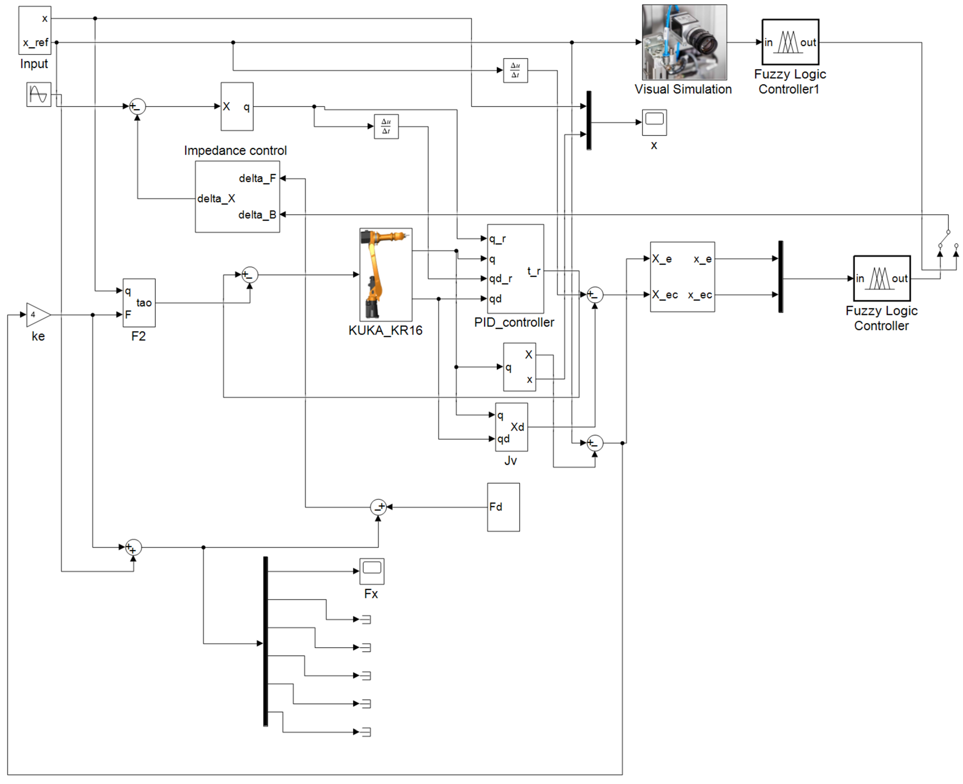
4.1. Simulation Design

In Solidworks 2020, a KUKA_KR16 robot model with six degrees of freedom was assembled and imported into Matlab/Simulink as shown in Figure 12. The initial position is [X, Y, Z] = [0, −930, 942] mm and the initial direction angle is [α, β, γ] = [0, 0, π/2]. The reference trajectory is a sinusoidal signal with a unit step size or amplitude of 1 mm and a frequency of 1 rad/s input along the X- direction of the fundamental robot coordinates at the tool center point of the robotic end effector. The position controller is PID controlled with k_p = 350, k_i = 80, and k_d = 150, and the impedance controller is parameterized with m_d = 1 and b_d = 600. The same control parameters are used for all joints. In the 2 s of the simulation, a disturbance force of 1 N is applied in the X direction. The basic ranges of the force error and force error rate in the fuzzy controller are [−0.5, 0.5] and [−1, 1], respectively. The damping parameter varies within [−400, 400]. The basic stiffness of the system in the X-direction is set to k_e = 4000 N/m. For the purpose of the investigation of the adaptation of the model to the system stiffness, the time-varying stiffness of the system is set to k_e = 4000 + 200sin(t). To simulate the potential errors that may occur in actual manufacturing and assembly processes, a 10% variation range was introduced to the inertial properties of the KUKA robot’s moving platform. Additionally, a 50 μm deviation value was added to its geometric properties to more realistically reflect the uncertainties in operation. The contact surface of the sliding platform was modeled as an elastic spring system with a stiffness coefficient set to 104 N/m. In the simulation experiments, a high-precision force sensor was installed on top of the robot’s end effector, with a measurement accuracy of ±1160 N in all three axes. To evaluate the stability of the control algorithm, a random disturbance of ±160 N was introduced into the force measurement output.

In this paper, a comparison is made among the traditional impedance control (TIC), fuzzy adaptive impedance control (FAIC), and adaptive impedance control based on visual guidance (AICVG). Figure 13 and Figure 14 present comprehensive comparisons of these three control methods under fixed and time-varying stiffness conditions, respectively.

In Figure 13, the reference line xd represents the desired displacement trajectory (system input command), while fd represents the desired contact force (force control target). The eight subfigures systematically compare displacement and force tracking performance: (Figure 13a,b) x-direction displacement tracking, (Figure 13c,d) corresponding tracking errors, (Figure 14a,b) z-direction force tracking, and (Figure 14c,d) associated force errors, with both step inputs (Figure 13a,c and Figure 14a,c) and sinusoidal inputs (Figure 13b,d and Figure 14b,d).

Under fixed stiffness conditions (Figure 13), the AICVG method (red curve) demonstrates superior performance in both displacement and force tracking. For displacement tracking, AICVG stabilizes to target positions within approximately 1 s with minimal overshoot, while TIC (green curve) requires about 2 s and exhibits significant overshoot. Quantitatively, AICVG maintains displacement steady-state errors within ±0.5 mm, compared to FAIC’s ±0.8 mm and TIC’s ±2 mm. For sinusoidal inputs, AICVG almost perfectly matches reference trajectories, while TIC displays obvious phase lag and amplitude attenuation.

In force tracking applications, the AICVG demonstrates rapid response to force variations, achieving stabilization within 0.5 s with minimal overshoot. In contrast, the TIC requires 2 s to stabilize and exhibits a 30% force overshoot. The steady-state force error for AICVG remains within ±1 N, whereas TIC errors reach ±4 N. When tracking sinusoidal force inputs, AICVG maintains precise force tracking with errors consistently within ±1.5 N, while TIC displays errors fluctuating within ±4 N accompanied by noticeable phase lag.

Figure 14 extends this comparison to time-varying stiffness conditions, where the system stiffness changes dynamically. The subfigure arrangement mirrors that of Figure 13, enabling direct comparison between fixed and variable stiffness scenarios. Under these more challenging conditions, AICVG maintains robust performance by rapidly adjusting control parameters to accommodate stiffness variations. For displacement tracking, AICVG stabilizes within 1.2 s despite stiffness fluctuations, with steady-state errors confined to ±0.8 mm. In contrast, TIC exhibits pronounced oscillations, requiring approximately 3 s to stabilize, with errors reaching ±3 mm and displaying distinct peaks at stiffness transition points.

For force tracking under time-varying stiffness conditions, AICVG stabilizes to the target force within approximately 0.8 s, confining errors to ±1.5 N even during stiffness transitions. In contrast, the FAIC method exhibits transient force fluctuations at stiffness change points but recovers within 1.2 s. TIC, however, fails to adapt effectively to stiffness variations, displaying persistent oscillations with errors reaching ±5 N and demonstrating poor stabilization performance.

The results conclusively demonstrate that the AICVG method exhibits superior displacement and force tracking performance under both fixed and time-varying stiffness conditions. This method responds rapidly to system changes while maintaining high-precision control, significantly outperforming the TIC approach. Although the FAIC method shows improvement over conventional methods, it remains inferior to the AICVG method in most scenarios. These findings validate the efficacy and superiority of the proposed vision-guided adaptive impedance control strategy for handling complex polishing tasks under varying environmental conditions.

The force-tracking performance over the 2–10 s interval is summarized in

Table 3. Comparison of force tracking performance.

Cases			Adjustment Time ts (s)	Maximum Overshoot Mp (%)	Error Integration Es (N·s)
Constant stiffness	Unit step	FAIC	0.271	1.1	0.193
		AICVG	0.256	0.5	0.161
		TIC	0.193	10.4	0.223
	Sine wave	FAIC	0.259	8.1	0.315
		AICVG	0.263	6.3	0.351
		TIC	0.185	12.1	0.642
Time-varying stiffness	Unit step	FAIC	0.237	9.7	0.272
		AICVG	0.244	0.8	0.177
		TIC	0.207	11.8	0.330
	Sine wave	FAIC	0.251	18.2	0.612
		AICVG	0.261	6.3	0.349
		TIC	0.258	23.2	0.671

. For systems with fixed stiffness, the results show that the adaptive impedance control method guided by visual feedback outperforms the other two strategies in terms of settling time, maximum overshoot, and integrated error. Similarly, in the case of time-varying stiffness, this method continues to demonstrate superior performance. Although its maximum overshoot is marginally higher than that of the fuzzy adaptive impedance control, the overall tracking error remains significantly lower.

These findings suggest that fuzzy impedance control also exhibits a strong ability to adapt to stiffness variations. However, it tends to produce larger steady-state errors and phase delays, despite achieving faster transient response. In contrast, the visually guided adaptive impedance control method offers enhanced tracking accuracy and stability across both fixed and varying stiffness conditions. Notably, when the system stiffness undergoes abrupt changes, this method proves more effective in suppressing force overshoot and oscillations.

Overall, the proposed visually guided adaptive impedance control approach integrates the advantages of rapid response and low error, making it particularly well-suited for dynamic environments with fluctuating stiffness.

4.2. Experimental Design

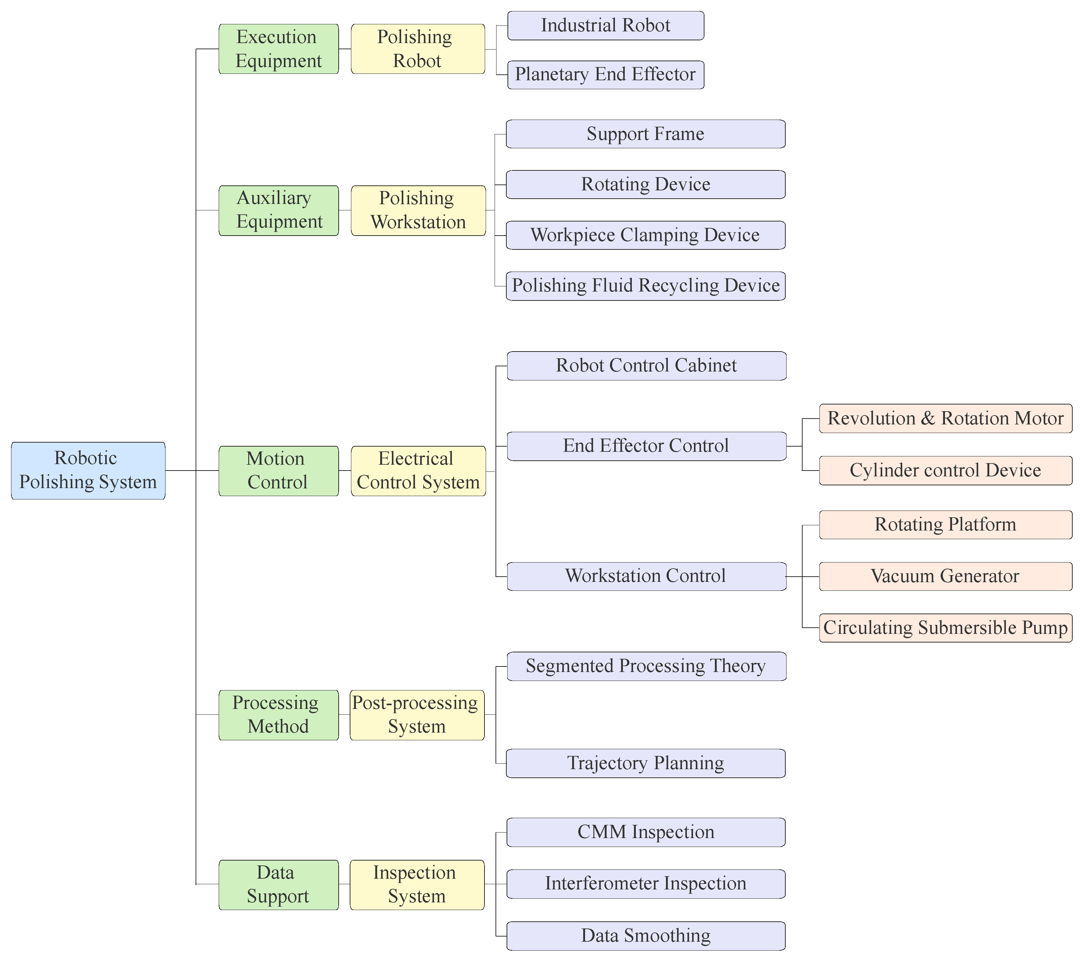
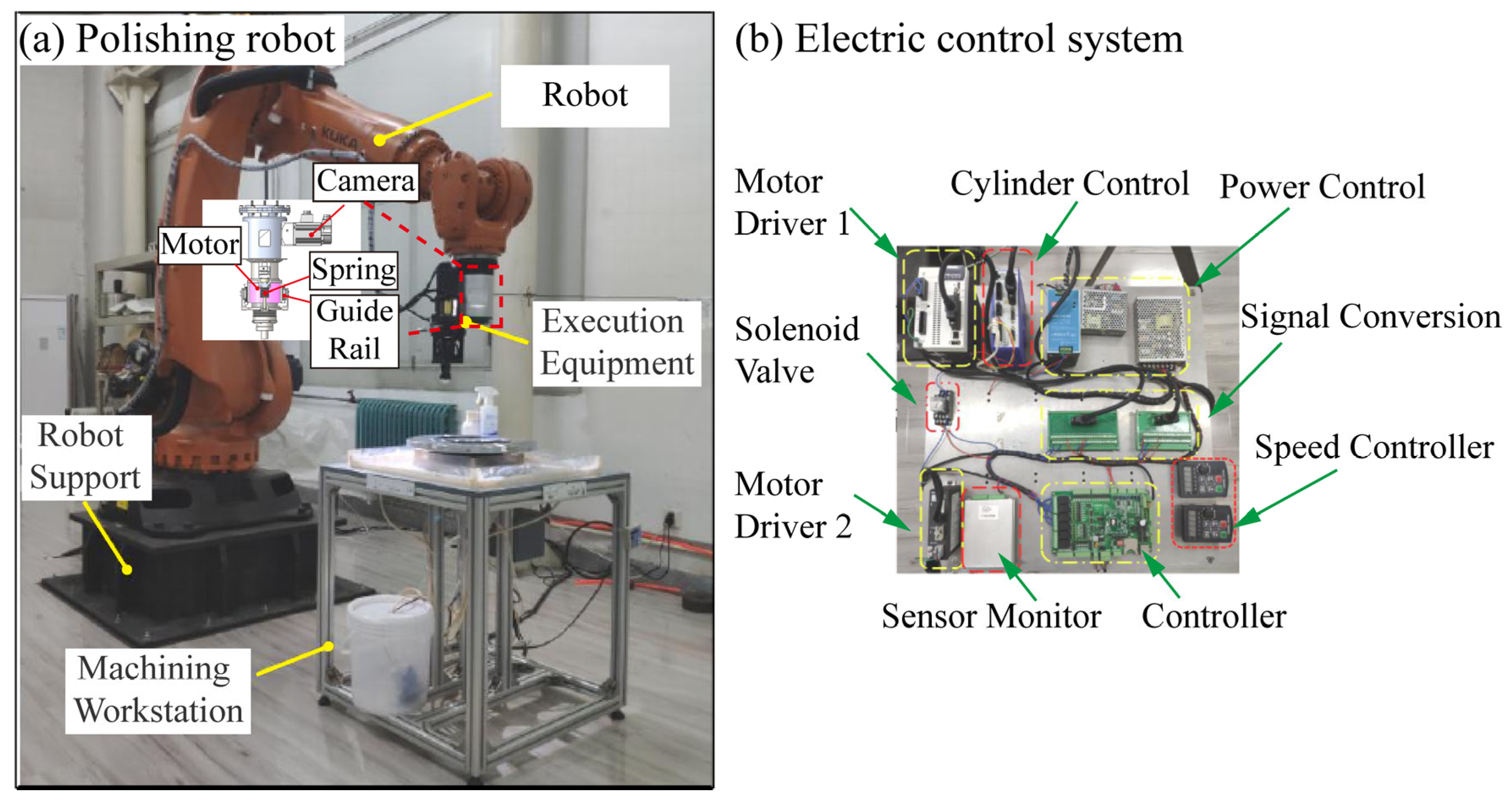
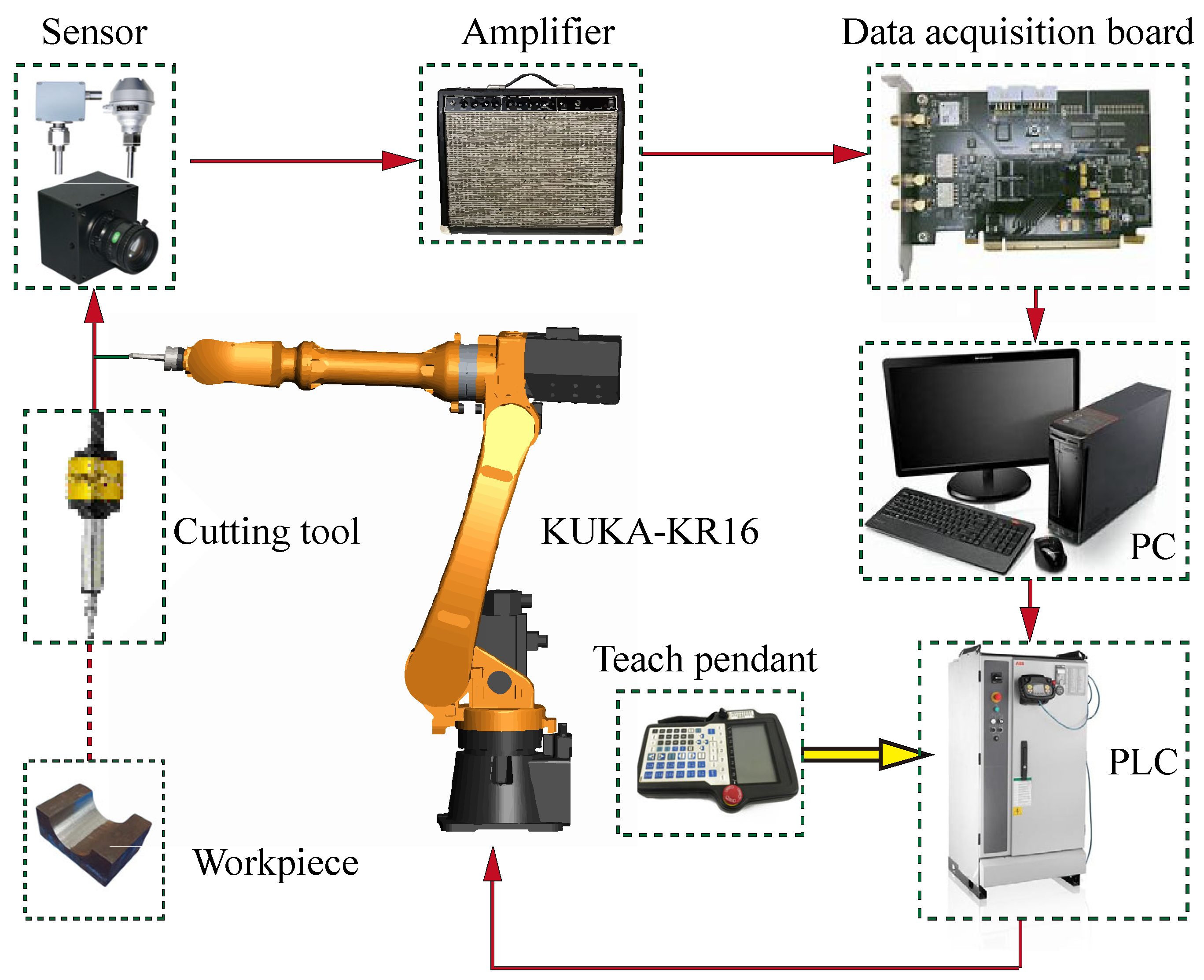
4.2.1. Robotic Polishing Platform

The robotic polishing system was constructed around a KUKA KR16 industrial robot, comprising mechanical, control, and auxiliary systems, and the detail composition of robotic polishing system is shown in Figure 15.

Table 4. Parameters table of the robot polishing experimental platform.

Parameter Category	Parameter Name	Parameter Value	Unit
Robot Body	Model	KUKA KR16	-
	Maximum Payload	16	kg
	Working Radius	1610	mm
	Repeatability	±0.05	mm
Sensors	Model	ATI Gamma SI-130-10	-
	Force Measurement Range	±130	N
	Torque Measurement Range	±10	Nm
	Sampling Frequency	1000	Hz
Polishing Tool	Type	Pneumatic Polishing Tool	-
	Polishing Head Diameter	50	mm
	Polishing Material	High-density Polyurethane	-
	Maximum Speed	12,000	rpm
Workpiece	Type	Concave Curved Surface Product	-
	Material	304 Stainless Steel	-
	Dimensions	200 × 150 × 50	mm
	Radius of Curvature	150	mm
Vision System	Camera Model	Basler acA2440-35uc	-
	Resolution	2448 × 2048	pixels
	Frame Rate	35	fps
Control Parameters	Polishing Speed	30–60	mm/s
	Polishing Force	20–40	N
	Force Control Accuracy	±1.5	N
	Control Cycle	1	ms
	Communication Period	0.012	s
	Visual Sampling Period	150	ms
	Force Sampling Period	6	ms

lists the key parameters of the KUKA KR16 robot polishing experimental platform in detail.

(1) Mechanical System

The primary mechanical component in this setup was a KUKA KR16 six-axis industrial robot (16 kg payload, 1610 mm reach, ±0.05 mm repeatability), which was mounted on a custom aluminum frame workbench (1500 mm × 800 mm × 750 mm, L × W × H). Workpieces were secured via a combination of vacuum suction and mechanical fixtures to ensure positional stability throughout machining. The polishing tool assembly employed a quick-change end effector and a standardized mounting plate, enabling rapid and reliable tool exchanges.

(2) Control System Architecture

The robotic system’s motion was managed by a KUKA KR C4 controller. Contact forces and torques were measured using an ATI Gamma SI-130-10 force/torque sensor mounted between the robot’s end flange and the polishing tool. Surface-feature recognition and real-time monitoring of the workpiece were achieved with a vision system comprising two Basler acA2440-35uc industrial cameras (2448 × 2048-pixel resolution). A host computer (Intel Core i7-10700, 32 GB RAM) executed the vision-guided fuzzy adaptive impedance control algorithm.

(3) Auxiliary Systems

The pneumatic supply delivered compressed air at 0.6–0.8 MPa to the polishing tool, while a closed-loop water-cooling circuit maintained stable workpiece surface temperatures. Uniform, shadow-free illumination for the vision system was provided by a ring-shaped LED light source. Operator safety was assured through photoelectric barriers, emergency-stop buttons, and protective fencing.

(4) Polishing Tool Configuration

A pneumatic spherical polishing tool with a 25 mm diameter head fabricated from high-density polyurethane was employed. The tool weighed 1.2 kg, reached up to 12,000 rpm, and operated at an air pressure of 0.6–0.7 MPa. It was affixed to a custom mounting plate coupled to the F/T sensor, allowing precise adjustment of polishing-head eccentricity and pitch angle. An integrated spring-damping mechanism provided an adjustable preload force ranging from 50 to 200 N.

(5) Workpiece Specifications and Fixturing

A small concave workpiece made from 304 stainless steel was used for all experiments. Its central region featured a concave curvature with a 150 mm radius, and the as-machined surface roughness measured approximately 1.2 μm. The workpiece coordinate system was defined with its origin at the geometric center. During testing, each workpiece was held in place by a vacuum-suction fixture exerting a clamping force of at least 500 N.

Figure 16a illustrates the spatial layout of the KUKA KR16 robot polishing experimental platform, while Figure 16b depicts the primary components of the electrical control system.

As shown in Figure 17, the polishing trajectories were generated offline in UG software through custom secondary-development modules. The workpiece surface was partitioned into discrete polishing zones, and within each zone the density and sequencing of polishing points were optimized to maintain smooth tool-pose continuity and maximize processing efficiency.

4.2.2. Experimental Parameters and Control Strategy

(1) Polishing Process Parameters

The polishing speed was maintained within a range of 30–60 mm/s, adjusted according to surface conditions. The tool posture was maintained with the Z-axis aligned perpendicular to the workpiece surface. An initial contact depth of 0.5 mm was established, with subsequent adjustments dynamically controlled by the impedance strategy. The spacing between adjacent polishing paths was set at 50% of the polishing head diameter.

(2) Force Control Parameters

The target polishing force was maintained within a range of 20–40 N, determined by material properties and surface specifications. The force control loop operated at a frequency of 1000 Hz. Force overshoot was constrained to a maximum of 15% of the setpoint, while steady-state fluctuations were maintained within ±1.5 N.

(3) Vision System Operational Parameters

The vision system operated at an image-acquisition rate of 30 frames per second (fps). The field of view measured 400 mm × 350 mm, resulting in a spatial resolution of 0.16 mm/pixel. The feature-recognition accuracy was ±0.2 mm.

(4) Fuzzy Adaptive Impedance Control Implementation

The fuzzy adaptive impedance controller was parameterized with the following Cartesian impedance matrices: mass matrix M = [5, 5, 5, 0.5, 0.5, 0.5] kg; damping matrix B = [300, 300, 300, 20, 20, 20] Ns/m; stiffness matrix K = [2000, 2000, 2000, 200, 200, 200] N/m. The fuzzy controller utilized force error (e) and force error change rate (ec) as inputs, producing an impedance parameter adjustment (ΔK) as output, based on 25 fuzzy rules. Adaptive parameters included a learning rate η = 0.05, a forgetting factor λ = 0.95, and an update period T = 0.001 s.

The fuzzy control domains for the vision-guided adaptive impedance control were: force error e₃(k)∈[−0.8, 0.8], change in force error Δe₃(k)∈[−1, 1], filtered force error ef₃(k)∈[−1, 1], change in desired displacement Δdd₃(k)∈[−6, 6], and change in stiffness Δkd₃(k)∈[−6, 6].

4.2.3. Control Strategy Validation

To validate the proposed control method, a robotic polishing system was utilized, as illustrated in Figure 18.

(1) System Configuration

The validation system consisted of a KUKA robotic arm, an electric spindle serving as the power unit, a computer, a teach pendant, and a robot control cabinet. The polishing tools included a spherical grinding wheel, a spherical rubber grinding head, and a wool felt wheel. The workpiece was a cylindrical component with a concave curvature. Predefined multi-axis toolpath data were imported into the host computer, which communicated with the robot controller at an interval of Δt = 0.012 s.

(2) Data Acquisition and Processing

Signal processing and data acquisition were conducted using an ME3DT120 triaxial force sensor, a PCIe-6351 data acquisition (DAQ) board, and a three-channel signal amplifier. The transducer output was amplified, processed by the DAQ board, and transmitted to a computer. The normal polishing force component was determined using Equation (17) after signal filtering. Impedance control parameters were derived from the force error and its rate of change. Subsequently, normal velocity compensation was computed via Equation (23) to adjust displacement along the surface normal direction.

(3) Visual Servoing Parameters for Validation

For the specific visual servoing tests conducted within this validation setup, the image resolution was set to 256 × 256 pixels. The experimental parameters were defined as L = 256 and W = 10. The sampling periods for the visual and force servo control tests were established at 150 ms and 6 ms, respectively.

(4) Visual Mapping Model Construction for Validation

To construct the visual mapping model for this validation, the robot performed pre-defined joint motions. A Charge-Coupled Device (CCD) camera, mounted on the robot’s end-effector, captured image features pertinent to curve tracking, from which the training dataset was compiled. During this data acquisition procedure, the end-effector tracked an unknown path while maintaining a constant contact force of 40 N.

The polishing process consists of three steps: rough polishing, semi-fine polishing and fine polishing, and the process parameters are shown in

Table 5. Parameters of the polishing process.

Processes	Tool Material	Speed (r/min)	Expected Force (N)	Feed Rate (mm/s)
rough polishing	Spherical grinding wheel	6000	6	18
semi-fine polishing	Spherical rubber	8000	4	18
fine polishing	Cylindrical Wool Felt	10,000	2	9

.

The sensors are used to measure the normal expected force of the tool for different processes. The comparison between the measured and the reference under the traditional impedance control, fuzzy adaptive impedance control, and vision-guided fuzzy adaptive impedance control are shown in Figure 19, Figure 20 and Figure 21, respectively. The comparison results indicate significant deviations and fluctuations between the measured and the reference of the traditional impedance control, resulting in unstable control. These force fluctuations typically manifest as chatter during the polishing process, leading to uneven material removal and compromised surface quality.

The unstable fluctuations and resulting chatter in the control process can be effectively reduced through the application of fuzzy adaptive impedance control, resulting in a more stable measured polishing force compared to traditional impedance control. Among the two strategies in which fuzzy adaptive impedance control is employed, the vision-guided-based solution obtains more stable polishing force and further minimizes chatter effects. The experimental results confirm that our proposed vision-guided fuzzy adaptive impedance control strategy successfully suppresses force fluctuations that would otherwise lead to chatter marks on the polished surface.

In conclusion, the vision-guided fuzzy adaptive impedance control offers significant advantages by reducing control force errors, eliminating chatter, and improving polishing quality, which provides valuable support for achieving efficient and stable polishing control. The reduction in the fluctuation of polishing force compared to traditional methods serves as quantitative evidence of the chatter suppression capabilities of our proposed approach.

The efficacy of the three control methods was further verified through surface quality evaluation. As illustrated in Figure 22, a comparative visualization of the workpiece surface before and after polishing reveals substantial improvement in smoothness. The workpiece was divided into polished and unpolished sections along its axis, with six measurement points (different color) selected from the polished region to assess surface roughness. The average value of these measurements was subsequently calculated.

Quantitative analysis conducted using a precision roughness meter revealed substantial performance variations among the three control strategies, as shown in

Table 6. Surface roughness comparison between three methods.

Method	Ra (μm)						Average Ra (μm)	Reduction Compared to TIC (%)
	1	2	3	4	5	6
TIC	0.090	0.100	0.095	0.080	0.110	0.047	0.087	-
FAIC	0.050	0.055	0.060	0.045	0.058	0.044	0.052	40.2%
AICVG	0.030	0.038	0.040	0.032	0.035	0.035	0.035	59.7%
Unpolished	-						3.75	-

.

The advanced control strategies achieved significantly lower surface roughness (Ra) compared to traditional impedance control (0.087 μm). Specifically, FAIC reduced surface roughness by 40.2% (0.052 μm), while AICVG demonstrated superior performance with a 59.7% reduction (0.035 μm). This hierarchical improvement in surface quality correlates directly with the force control capabilities observed in tracking experiments (Figure 13 and Figure 14), where both advanced methods exhibited progressively reduced force fluctuations, with AICVG consistently outperforming FAIC.

Experimental evaluations confirm that the vision-guided approach offers substantial advantages in both dynamic response and surface quality. These benefits are particularly pronounced under time-varying stiffness conditions, where AICVG’s superior adaptive capabilities directly enhance surface finish.

These results demonstrate conclusively that advanced adaptive control strategies significantly enhance surface quality in robotic polishing applications, with the vision-guided approach yielding the most substantial improvements. The quantitative relationship between control method sophistication and surface quality enhancement suggests promising applications for high-precision manufacturing across various industries.

5. Conclusions

This study developed and validated a novel adaptive impedance control based on visual guidance (AICVG) strategy to address the challenges of robotic polishing on curved workpieces with time-varying stiffness. This approach integrates visual servoing, which provides real-time geometric information and compensates for tool path deviations, with a fuzzy adaptive impedance controller that dynamically adjusts control parameters in response to varying contact conditions.

Comparative simulations and experiments demonstrated that AICVG outperforms both traditional impedance control (TIC) and fuzzy adaptive impedance control (FAIC) in maintaining stable contact forces, particularly during abrupt stiffness variations. The method effectively suppressed force overshoot and minimized steady-state fluctuations, limiting the maximum force control error to ±1.5 N. This improvement in force regulation directly enhanced surface quality, with AICVG achieving a 60% reduction in surface roughness compared to TIC and a significant improvement over FAIC.

The results demonstrate the system’s ability to adapt to uncertain and dynamic polishing environments, addressing a key limitation of existing robotic polishing technologies. By effectively managing the interaction between the robot, tool, and workpiece, AICVG provides a robust and precise solution for automated polishing of complex curved surfaces. Future research could explore machine learning for stiffness prediction and further optimization of adaptive control parameters.

References

1. Perez Dewey, M.; Ulutan, D. Development of Laser Polishing as an Auxiliary Post-Process to Improve Surface Quality in Fused Deposition Modeling Parts. In Proceedings of the International Manufacturing Science and Engineering Conference, American Society of Mechanical Engineers, Los Angeles, CA, USA, 4–8 June 2017; Volume 50732, p. V002T01A006. [Google Scholar]
2. Tian, F.; Li, Z.; Lv, C.; Liu, G. Polishing Pressure Investigations of Robot Automatic Polishing on Curved Surfaces. Int. J. Adv. Manuf. Technol. 2016, 87, 639–646. [Google Scholar] [CrossRef]
3. Ermergen, T.; Taylan, F. Review on Surface Quality Improvement of Additively Manufactured Metals by Laser Polishing. Arab. J. Sci. Eng. 2021, 46, 7125–7141. [Google Scholar] [CrossRef]
4. Ferraguti, F.; Pini, F.; Gale, T.; Messmer, F.; Storchi, C.; Leali, F.; Fantuzzi, C. Augmented Reality Based Approach for On-Line Quality Assessment of Polished Surfaces. Robot. Comput.-Integr. Manuf. 2019, 59, 158–167. [Google Scholar] [CrossRef]
5. Khalick Mohammad, A.E.; Hong, J.; Wang, D. Polishing of Uneven Surfaces Using Industrial Robots Based on Neural Network and Genetic Algorithm. Int. J. Adv. Manuf. Technol. 2017, 93, 1463–1471. [Google Scholar] [CrossRef]
6. Caggiano, A.; Teti, R.; Alfieri, V.; Caiazzo, F. Automated Laser Polishing for Surface Finish Enhancement of Additive Manufactured Components for the Automotive Industry. Prod. Eng. 2021, 15, 109–117. [Google Scholar] [CrossRef]
7. Oba, Y.; Kakinuma, Y. Simultaneous Tool Posture and Polishing Force Control of Unknown Curved Surface Using Serial-Parallel Mechanism Polishing Machine. Precis. Eng. 2017, 49, 24–32. [Google Scholar] [CrossRef]
8. Xiao, G.; Huang, Y.; Yin, J. An Integrated Polishing Method for Compressor Blade Surfaces. Int. J. Adv. Manuf. Technol. 2017, 88, 1723–1733. [Google Scholar] [CrossRef]
9. Lim, M.S.H. Digitalization of Mass Vibratory Polishing Process for Aerospace Application; Nanyang Technological University: Singapore, 2022. [Google Scholar]
10. Krishnan, A.; Fang, F. Review on Mechanism and Process of Surface Polishing Using Lasers. Front. Mech. Eng. 2019, 14, 299–319. [Google Scholar] [CrossRef]
11. Zhu, P.; Han, J.; Xie, H.; Li, X. Study of Ultrafast Laser Polishing Technology. In Proceedings of the International Conference on Photonics and Optical Engineering (icPOE 2014), Xi’an, China, 13–15 October 2014; SPIE: Bellingham, WA, USA, 2015; Volume 9449, pp. 821–825. [Google Scholar]
12. Tian, F.; Lv, C.; Li, Z.; Liu, G. Modeling and Control of Robotic Automatic Polishing for Curved Surfaces. CIRP J. Manuf. Sci. Technol. 2016, 14, 55–64. [Google Scholar] [CrossRef]
13. Walker, D.; Yu, G.Y.; Gray, C.; Rees, P.; Bibby, M.; Wu, H.Y.; Zheng, X. Process Automation in Computer Controlled Polishing. Adv. Mater. Res. 2016, 1136, 684–689. [Google Scholar] [CrossRef]
14. Su, Z.; Ying, Z. Polishing Path Planning of Complex Curved Surfaces and the Realization of Automatic Control. Int. J. Smart Home 2016, 10, 233–240. [Google Scholar] [CrossRef]
15. Wei, Y.; Xu, Q. Design of a New Passive End-Effector Based on Constant-Force Mechanism for Robotic Polishing. Robot. Comput.-Integr. Manuf. 2022, 74, 102278. [Google Scholar] [CrossRef]
16. Zhang, X.; Sun, Y. Development of Pneumatic Force-Controlled Actuator for Automatic Robot Polishing Complex Curved Plexiglass Parts. Machines 2023, 11, 446. [Google Scholar] [CrossRef]
17. Li, J.; Guan, Y.; Chen, H.; Wang, B.; Zhang, T.; Liu, X.; Hong, J.; Wang, D.; Zhang, H. A High-Bandwidth End-Effector with Active Force Control for Robotic Polishing. IEEE Access 2020, 8, 169122–169135. [Google Scholar] [CrossRef]
18. Lakshminarayanan, S.; Kana, S.; Mohan, D.M.; Manyar, O.M.; Then, D.; Campolo, D. An Adaptive Framework for Robotic Polishing Based on Impedance Control. Int. J. Adv. Manuf. Technol. 2021, 112, 401–417. [Google Scholar] [CrossRef]
19. Ochoa, H.; Cortesão, R. Impedance Control Architecture for Robotic-Assisted Mold Polishing Based on Human Demonstration. IEEE Trans. Ind. Electron. 2021, 69, 3822–3830. [Google Scholar] [CrossRef]
20. Ding, Y.; Zhao, J.; Min, X. Impedance Control and Parameter Optimization of Surface Polishing Robot Based on Reinforcement Learning. Proc. Inst. Mech. Eng. Part B J. Eng. Manuf. 2023, 237, 216–228. [Google Scholar] [CrossRef]
21. Xiao, C.; Wang, Q.; Zhou, X.; Xu, Z.; Lao, X.; Chen, Y. Hybrid Force/Position Control Strategy for Electromagnetic Based Robotic Polishing Systems. In Proceedings of the 2019 Chinese Control Conference (CCC), Guangzhou, China, 27–30 July 2019; pp. 7010–7015. [Google Scholar]
22. Gracia, L.; Solanes, J.E.; Muñoz-Benavent, P.; Valls Miro, J.; Perez-Vidal, C.; Tornero, J. Adaptive Sliding Mode Control for Robotic Surface Treatment Using Force Feedback. Mechatronics 2018, 52, 102–118. [Google Scholar] [CrossRef]
23. Gal, I.-A.; Ciocîrlan, A.-C.; Mărgăritescu, M. State Machine-Based Hybrid Position/Force Control Architecture for a Waste Management Mobile Robot with 5DOF Manipulator. Appl. Sci. 2021, 11, 4222. [Google Scholar] [CrossRef]
24. Luo, Z.; Li, J.; Bai, J.; Wang, Y.; Liu, L. Adaptive Hybrid Impedance Control Algorithm Based on Subsystem Dynamics Model for Robot Polishing. In Proceedings of the Intelligent Robotics and Applications: 12th International Conference, ICIRA 2019, Shenyang, China, 8–11 August 2019; Proceedings, Part VI 12. Springer: Berlin/Heidelberg, Germany, 2019; pp. 163–176. [Google Scholar]
25. Zhou, H.; Ma, S.; Wang, G.; Deng, Y.; Liu, Z. A Hybrid Control Strategy for Grinding and Polishing Robot Based on Adaptive Impedance Control. Adv. Mech. Eng. 2021, 13, 16878140211004034. [Google Scholar] [CrossRef]
26. Koivumäki, J.; Mattila, J. Stability-Guaranteed Impedance Control of Hydraulic Robotic Manipulators. IEEE/ASME Trans. Mechatron. 2016, 22, 601–612. [Google Scholar] [CrossRef]
27. Luo, Z.; Yang, S.; Sun, Y.; Liu, H. Optimized Control for Dynamical Performance of the Polishing Robot in Unstructured Environment. Shock Vib. 2011, 18, 355–364. [Google Scholar] [CrossRef]
28. Hamedani, M.H.; Sadeghian, H.; Zekri, M.; Sheikholeslam, F.; Keshmiri, M. Intelligent Impedance Control Using Wavelet Neural Network for Dynamic Contact Force Tracking in Unknown Varying Environments. Control Eng. Pract. 2021, 113, 104840. [Google Scholar] [CrossRef]
29. Hamedani, M.H.; Zekri, M.; Sheikholeslam, F.; Selvaggio, M.; Ficuciello, F.; Siciliano, B. Recurrent Fuzzy Wavelet Neural Network Variable Impedance Control of Robotic Manipulators with Fuzzy Gain Dynamic Surface in an Unknown Varied Environment. Fuzzy Sets Syst. 2021, 416, 1–26. [Google Scholar] [CrossRef]
30. Cao, H. Design of a Fuzzy Fractional Order Adaptive Impedance Controller with Integer Order Approximation for Stable Robotic Contact Force Tracking in Uncertain Environment. Acta Mech. Autom. 2022, 16, 16–26. [Google Scholar] [CrossRef]
31. Li, Z.; Huang, H.; Song, X.; Xu, W.; Li, B. A Fuzzy Adaptive Admittance Controller for Force Tracking in an Uncertain Contact Environment. IET Control Theory Appl. 2021, 15, 2158–2170. [Google Scholar] [CrossRef]
32. Mazare, M.; Tolu, S.; Taghizadeh, M. Adaptive Variable Impedance Control for a Modular Soft Robot Manipulator in Configuration Space. Meccanica 2022, 57, 1–15. [Google Scholar] [CrossRef]
33. Cao, H.; Zhou, J.; Jiang, P.; Hon, K.K.B.; Yi, H.; Dong, C. An Integrated Processing Energy Modeling and Optimization of Automated Robotic Polishing System. Robot. Comput.-Integr. Manuf. 2020, 65, 101973. [Google Scholar] [CrossRef]
34. Ding, Y.; Min, X.; Fu, W.; Liang, Z. Research and Application on Force Control of Industrial Robot Polishing Concave Curved Surfaces. Proc. Inst. Mech. Eng. Part B J. Eng. Manuf. 2019, 233, 1674–1686. [Google Scholar] [CrossRef]
35. Nagata, F.; Hase, T.; Haga, Z.; Omoto, M.; Watanabe, K. CAD/CAM-Based Position/Force Controller for a Mold Polishing Robot. Mechatronics 2007, 17, 207–216. [Google Scholar] [CrossRef]
36. Yang, L.; Zhang, Y.; Han, Y.; Zhang, B.; Wang, Z. Robot Automatic Polishing Technology of Curved Parts Based on Adaptive Impedance Control. In Proceedings of the International Conference on Mechanism and Machine Science, Yantai, China, 30 July–1 August 2022; Springer: Berlin/Heidelberg, Germany, 2022; pp. 2073–2086. [Google Scholar]
37. Huang, Y.; Chen, H.; Cui, Z.; Zhang, X. An Adaptive Impedance Control Method for Human-Robot Interaction. In Proceedings of the International Conference on Intelligent Robotics and Applications, Hangzhou, China, 5–7 July 2023; Springer: Berlin/Heidelberg, Germany, 2023; pp. 529–539. [Google Scholar]
38. Sheng, X.; Zhang, X. Fuzzy Adaptive Hybrid Impedance Control for Mirror Milling System. Mechatronics 2018, 53, 20–27. [Google Scholar] [CrossRef]
39. Duan, J.; Gan, Y.; Chen, M.; Dai, X. Adaptive Variable Impedance Control for Dynamic Contact Force Tracking in Uncertain Environment. Robot. Auton. Syst. 2018, 102, 54–65. [Google Scholar] [CrossRef]
40. Shen, Y.; Lu, Y.; Zhuang, C. A Fuzzy-Based Impedance Control for Force Tracking in Unknown Environment. J. Mech. Sci. Technol. 2022, 36, 5231–5242. [Google Scholar] [CrossRef]
41. Ahmadi, B.; Xie, W.; Zakeri, E. Robust cascade vision/force control of industrial robots utilizing continuous integral sliding-mode control method. IEEE/ASME Trans. Mechatron. 2021, 27, 524–536. [Google Scholar] [CrossRef]
42. Zhou, F.; Liu, H.; Zhang, P.; Ouyang, X.; Xu, L.; Ge, Y.; Yao, Y.; Yang, H. High-Precision Control Solution for Asymmetrical Electro-Hydrostatic Actuators Based on the Three-Port Pump and Disturbance Observers. IEEE/ASME Trans. Mechatron. 2023, 28, 396–406. [Google Scholar] [CrossRef]
43. Thuilot, B.; Martinet, P.; Cordesses, L.; Gallice, J. Position Based Visual Servoing: Keeping the Object in the Field of Vision. In Proceedings of the 2002 IEEE International Conference on Robotics and Automation (Cat. No. 02CH37292), Washington, DC, USA, 11–15 May 2002; IEEE: New York, NY, USA, 2002; Volume 2, pp. 1624–1629. [Google Scholar]
Figure 1. Schematic diagram of tool compensation.
Machines 13 00493 g001
Figure 2. Schematic diagram of the tool position during the polishing procedure.
Machines 13 00493 g002
Figure 3. Schematic diagram of normal vector interpolation.
Machines 13 00493 g003
Figure 4. Force analysis of during the polishing.
Machines 13 00493 g004
Figure 5. Schematic diagram of gravity compensation.
Machines 13 00493 g005
Figure 6. The block diagram of position-based impedance control.
Machines 13 00493 g006
Figure 7. Schematic diagram of displacement compensation and force.
Machines 13 00493 g007
Figure 8. The relationship of normal polishing force and displacement.
Machines 13 00493 g008
Figure 9. The block diagram of fuzzy adaptive impedance control.
Machines 13 00493 g009
Figure 10. Schematic diagram of impedance vision force control.
Machines 13 00493 g010
Figure 11. Definition of image feature parameter vector.
Machines 13 00493 g011
Figure 12. The simulation model of polishing robotic systems.
Machines 13 00493 g012
Figure 13. Comparison of the control results under fixed stiffness.
Machines 13 00493 g013
Figure 14. Comparison of the control results under time-varying stiffness.
Machines 13 00493 g014
Figure 15. Composition of robotic polishing system.
Machines 13 00493 g015
Figure 16. Overall schematic of the KUKA KR16 robotic polishing experimental platform: (a) Spatial layout of the polishing robot; (b) Key components of the electrical control system.
Machines 13 00493 g016
Figure 17. Surface polishing trajectory.
Machines 13 00493 g017
Figure 18. Schematic diagram of the experimental setup.
Machines 13 00493 g018
Figure 19. The polishing force of traditional impedance control.
Machines 13 00493 g019
Figure 20. The polishing force of fuzzy adaptive impedance control.
Machines 13 00493 g020
Figure 21. The polishing force of vision-guided fuzzy adaptive impedance control.
Machines 13 00493 g021
Figure 22. The comparison of workpiece surface before and after polishing.
Machines 13 00493 g022