Robust Self-Calibration of Subreflector Actuators Under Noise and Limited Workspace Conditions

Abstract

Accurate kinematic calibration of subreflector actuators is essential for pointing precision of large radio telescopes, particularly at high frequencies. Conventional least-squares methods are vulnerable to noise and outliers, and their accuracy may degrade when limited pose diversity leads to poor parameter excitation. To address these challenges, this paper proposes a novel robust self-calibration framework that integrates Huber loss and $L_2$ regularization into the Levenberg–Marquardt (LM) algorithm—yielding a hybrid optimization approach that combines residual robustness, numerical stability, and convergence reliability. A comprehensive simulation study was conducted under varying workspace sizes and sensor noise levels. The proposed method maintained stable performance even under reduced excitation and high-noise conditions, where traditional LM methods typically degrade, confirming its robustness and applicability to realistic calibration scenarios. The framework was further validated using a structured-light 6-DOF pose measurement system, the proposed method achieved over 90% improvement in both position and orientation accuracy compared to the traditional LM approach. These findings confirm the method’s effectiveness for high-precision 6-DOF calibration in parallel mechanisms, and its suitability for real-world applications in radio telescope subreflector alignment.

1. Introduction

Radio telescopes are essential instruments in modern astronomy, enabling the detection and analysis of radio waves emitted by celestial objects. To optimize their sensitivity and resolution, many radio telescopes employ a dual-reflector design, consisting of a large primary mirror that collects incoming radio waves and a smaller secondary mirror, known as the subreflector, which focuses these waves onto a receiver system [1]. The precise positioning of the subreflector is crucial, as even slight misalignments can significantly degrade the telescope’s performance [2]. However, due to the impact of environmental factors such as gravity and temperature, the structural deformation of a telescope can lead to misalignment between the subreflector and primary reflector.

To achieve the necessary precision, modern radio telescopes often utilize 6-Degree Of Freedom (6-DOF) parallel platforms as subreflector actuators to adjust the subreflector’s position and orientation [3]. The QiTai Radio Telescope (QTT), currently under construction, features a Gregorian parabolic antenna designed to cover the frequency range of 150 MHz to 115 GHz, a subreflector that is an aluminum honeycomb sandwich structure, an aperture of 12 m, and a weight of about 4000 kg, and its geometric surface is a hyperboloid of revolution [4,5]. The subreflector of QTT employs an asymmetric Stewart platform to achieve the desired position and orientation through precise control of each actuator’s length [6]. The Green Bank Radio Telescope (GBT) also uses an orthogonal Stewart platform as a subreflector actuator [7]. Additionally, in 2006, the 100 m Effelsberg telescope was upgraded with an active subreflector system that implemented an asymmetric Stewart platform to ensure the accurate positioning and orientation of the subreflector [8]. Several well-known radio telescopes have successfully applied traditional Stewart platforms, including the Large Millimeter Telescope (LMT) [9], the Atacama Large Millimeter Array (ALMA) [10], the Five-hundred-meter Aperture Spherical Telescope (FAST) [11], the TianMa Radio Telescope [12], and the NanShan Radio Telescope (NSRT) [13], among others.

Radio telescopes, often located in remote areas, face environmental challenges like gravity, solar radiation, and wind loads, which, along with internal wear and temperature fluctuations, cause distortions in subreflector actuators. These factors lead to increased joint clearances, thermal deformation, and pose errors, impacting the platform’s accuracy and operational stability [14,15,16]. This paper attempts to solve this problem via the proposed kinematic calibration method for the subreflector actuator. Kinematic calibration is widely used for various robots, which can effectively and economically improve the kinematic accuracy of robots without changing hardware [17,18]. The least-squares method (LSM) is widely used in robotic calibration for linear and nonlinear error modeling. It estimates parameters by minimizing the sum of squared residuals between measured and predicted data [19]. The Levenberg–Marquardt (LM) algorithm is a hybrid between the Gauss–Newton method and gradient descent, offering a powerful nonlinear optimization approach for calibration [20]. Beyond traditional optimization methods, evolutionary algorithms have gained traction for their global search capabilities in kinematic parameter identification. Zhang et al. compared GA and PSO to address the complexity of parameter calibration problems [21]. Huang et al. combined geometric and nongeometric errors into a normalized model optimized via GA% [22].

Traditional calibration techniques, while effective in ideal conditions, often struggle with the sensitivity to initial conditions, local minima convergence, and susceptibility to measurement noise. These limitations hinder their performance, especially in dynamic environments with complex nonlinearities. To address these challenges, recent studies have introduced hybrid approaches that combine the strengths of multiple optimization techniques. Nguyen et al. improved robot precision positioning using a neural network based on the LM-APSO algorithm [23]. Yu developed an improved particle swarm optimization (PSO) algorithm to enhance positioning and orientation accuracy of the parallel robot for spacecraft docking simulation system [24]. Similarly, Wang et al. explored the use of iterative Extended Kalman Filtering (EKF) in real-time kinematic calibration for a Stewart platform, making it highly suitable for systems subjected to varying conditions [25]. Feng et al. proposed combining LM and the improved Marine Predators algorithm, which significantly reduced the positioning error [26]. These studies highlight the growing complexity of calibration tasks and emphasize the need for sophisticated, hybrid strategies capable of handling noisy measurements and nonlinear dynamics.

The Huber loss function offers a promising approach for handling outliers and noise, which is particularly relevant for environments with unpredictable disturbances. Sun et al. applied Huber loss to robust calibration of computer models [27]. Liu et al. introduced an $L_2$-regularization-based method for industrial robot calibration in limited measurement spaces, offering insights into addressing workspace constraints [28]. These studies underscore the potential of combining Levenberg–Marquardt optimization, $L_2$ regularization, and Huber loss to develop robust calibration frameworks for subreflector actuators, ensuring precision and stability under challenging conditions.

Building upon these foundational insights, this study proposes a novel robust calibration framework that integrates Huber loss, $L_2$ regularization, and the LM algorithm. Huber loss mitigates the influence of outliers, while $L_2$ regularization enhances stability under limited measurement conditions—such as when the visible region of the tracking system is smaller than the actuator’s full mechanical workspace. The LM algorithm ensures efficient and reliable convergence, even in the presence of noise. Pose measurements are obtained using a structured-light optical system that projects a laser grid and reconstructs 6-DOF poses from observed spot deformations. The proposed method enables accurate and repeatable identification of kinematic parameters in complex parallel mechanisms, such as subreflector actuators in large radio telescopes. Moreover, the proposed robust calibration framework is broadly applicable to other complex systems—such as robotic manipulators and aerospace positioning systems—that demand high-precision kinematic calibration under noisy, limited-data conditions.

The paper is organized as follows: Section 2 introduces the subreflector actuator and its mathematical model; Section 3 presents the robust identification method; Section 4 describes the calibration experiments; Section 5 discusses the results; and Section 6 concludes the study with key findings and future directions.

2. Subreflector Actuator of the Radio Telescopes and Its Mathematical Model

2.1. Structural Configuration

The subreflector of the radio telescopes has six degrees of freedom, five of which are controlled by the 6-DOF parallel platform (the rotation around the z-axis is not considered because of the axisymmetrical shape of the subreflector). The subreflector is supported on the primary reflector by 4 orthogonal supporting legs and the angles between the elevation axis and legs in the elevation axis plane projection are ±45° and ±135°, respectively. The elevation range of the primary reflector during observations is 5° to 88°. Any positional offset of the subreflector induces pointing deviations in the radio telescope, necessitating exceptional positional and orientational accuracy across diverse operating conditions.

The actuator design ensures high stiffness and load capacity, essential for maintaining subreflector stability under varying environmental conditions. However, subreflector actuators are affected by harsh environmental factors. Additionally, prolonged operation accelerates internal wear, increasing joint clearances and reducing transmission accuracy. Temperature fluctuations cause thermal deformation in components like actuators and joints, distorting the relationship between the platform’s pose and motor displacements. Gravity loads fluctuate with the elevation angle, further affecting joint clearances. These distortions introduce pose errors, preventing the subreflector from achieving the required position and orientation. We aim to address this issue through the proposed kinematic calibration method, and through periodic kinematic calibration, compensate for the errors of the subreflector actuator.

The subreflector actuator consists of a fixed base platform and a movable platform connected by six extensible legs, as illustrated in Figure 1. The base platform is rigidly mounted to the telescope’s supporting structure, while the movable platform supports the subreflector. Each leg is equipped with a high-precision linear actuator capable of extending or contracting to adjust the subreflector’s pose. The nominal geometry includes six base joints (${\mathbf{b}}_i$, $i=1,2,\dots ,6$) and six platform joints (${\mathbf{p}}_i$), whose coordinates are defined in their respective coordinate systems—the base coordinate system (BCS) and platform coordinate system (PCS).

2.2. Kinematic Model

The kinematic model of the subreflector actuator relates the pose of the movable platform to the lengths of its six legs, forming the basis for kinematic calibration. The platform pose in BCS is denoted as:

$$\mathbf{q}={[x,y,z,\alpha ,\beta ,\gamma ]}^T=[\mathbf{t},\mathbf{s}]$$

(1)

where $\mathbf{t}={[x,y,z]}^T$ is the translation vector and $\mathbf{s}={[\alpha ,\beta ,\gamma ]}^T$ represents the Euler angles (rotation vector).

Inverse kinematics given the platform pose $(\mathbf{t},\mathbf{s})$ solves the nominal leg vector ${\mathbf{L}}_i$ for the i-th leg ($i=1,2,\dots ,6$) as:

$${\mathbf{L}}_i=\mathbf{t}+\mathbf{R}{\mathbf{p}}_i-{\mathbf{b}}_i$$

(2)

where:

• ${\mathbf{p}}_i={[p_{xi},p_{yi},p_{zi}]}^T$: coordinates of the platform joints in the PCS.
• ${\mathbf{b}}_i={[b_{xi},b_{yi},b_{zi}]}^T$: coordinates of the base joints in BCS.
• $\mathbf{R}$: Rotation matrix derived from ZYX Euler angles:

  $$\mathbf{R}=\left[\begin{array}{ccc}cos\gamma cos\beta & cos\gamma sin\beta sin\alpha -sin\gamma cos\alpha & cos\gamma sin\beta cos\alpha +sin\gamma sin\alpha \\ sin\gamma cos\beta & sin\gamma sin\beta sin\alpha +cos\gamma cos\alpha & sin\gamma sin\beta cos\alpha -cos\gamma sin\alpha \\ -sin\beta & cos\beta sin\alpha & cos\beta cos\alpha \end{array}\right]$$

  (3)

The nominal leg length $l_i$ is:

$$l_i=\parallel {\mathbf{L}}_i\parallel =\sqrt{{\mathbf{L}}_i^T{\mathbf{L}}_i}$$

(4)

Given the leg lengths $\mathbf{l}={[l_1,l_2,l_3,l_4,l_5,l_6]}^T$, the forward kinematics solves $\mathbf{t}$ and $\mathbf{R}$ (or equivalently $\mathbf{q}$). This is a nonlinear problem due to the square root in the length equation, and it is addressed iteratively using the Gauss–Newton method. The process minimizes the difference between the given leg lengths and those computed from the pose.

The forward kinematics is formulated by defining the residual function for each leg:

$$f_i\left(\mathbf{q}\right)=l_i-\sqrt{{(\mathbf{t}+\mathbf{R}{\mathbf{p}}_i-{\mathbf{b}}_i)}^T(\mathbf{t}+\mathbf{R}{\mathbf{p}}_i-{\mathbf{b}}_i)}$$

(5)

The objective is to find $\mathbf{q}$ such that the total squared residual is minimized:

$$F\left(\mathbf{q}\right)=\sum _{i=1}^6{f}_i{\left(\mathbf{q}\right)}^2$$

(6)

Vectorizing the residuals:

$$\mathbf{f}\left(\mathbf{q}\right)={[f_1\left(\mathbf{q}\right),f_2\left(\mathbf{q}\right),f_3\left(\mathbf{q}\right),f_4\left(\mathbf{q}\right),f_5\left(\mathbf{q}\right),f_6\left(\mathbf{q}\right)]}^T$$

(7)

Thus:

$$F\left(\mathbf{q}\right)=\mathbf{f}{\left(\mathbf{q}\right)}^T\mathbf{f}\left(\mathbf{q}\right)$$

(8)

The Gauss–Newton iteration proceeds as follows:

(1)

Initial Guess: Assume an initial pose ${\mathbf{q}}_0={[x_0,y_0,z_0,{\alpha }_0,{\beta }_0,{\gamma }_0]}^T$, and set a convergence threshold $ϵ>0$. Initialize iteration counter $k=0$.

(2)

Residual Calculation: Compute the residual vector ${\mathbf{f}}_k=\mathbf{f}\left({\mathbf{q}}_k\right)$ at iteration k:

$${\mathbf{f}}_k=[l_1-\parallel {\mathbf{L}}_1\left({\mathbf{q}}_k\right)\parallel ,l_2-\parallel {\mathbf{L}}_2\left({\mathbf{q}}_k\right)\parallel ,\dots ,l_6-\parallel {\mathbf{L}}_6\left({\mathbf{q}}_k\right){\parallel ]}^T$$

(9)

where ${\mathbf{L}}_i\left({\mathbf{q}}_k\right)={\mathbf{t}}_k+{\mathbf{R}}_k{\mathbf{p}}_i-{\mathbf{b}}_i$, and ${\mathbf{t}}_k,{\mathbf{R}}_k$ are derived from ${\mathbf{q}}_k$.

(3)

Jacobian Matrix: Construct the $6\times 6$ Jacobian ${\mathbf{J}}_k={\displaystyle \frac{\partial \mathbf{f}}{\partial \mathbf{q}}}{|}_{{\mathbf{q}}_k}$, where each element is:

$${\mathbf{J}}_k=\left[\begin{array}{cccccc}{\displaystyle \frac{\partial f_1}{\partial x}}& {\displaystyle \frac{\partial f_1}{\partial y}}& {\displaystyle \frac{\partial f_1}{\partial z}}& {\displaystyle \frac{\partial f_1}{\partial \alpha }}& {\displaystyle \frac{\partial f_1}{\partial \beta }}& {\displaystyle \frac{\partial f_1}{\partial \gamma }}\\ {\displaystyle \frac{\partial f_2}{\partial x}}& {\displaystyle \frac{\partial f_2}{\partial y}}& {\displaystyle \frac{\partial f_2}{\partial z}}& {\displaystyle \frac{\partial f_2}{\partial \alpha }}& {\displaystyle \frac{\partial f_2}{\partial \beta }}& {\displaystyle \frac{\partial f_2}{\partial \gamma }}\\ ⋮& ⋮& ⋮& ⋮& ⋮& ⋮\\ {\displaystyle \frac{\partial f_6}{\partial x}}& {\displaystyle \frac{\partial f_6}{\partial y}}& {\displaystyle \frac{\partial f_6}{\partial z}}& {\displaystyle \frac{\partial f_6}{\partial \alpha }}& {\displaystyle \frac{\partial f_6}{\partial \beta }}& {\displaystyle \frac{\partial f_6}{\partial \gamma }}\end{array}\right]$$

(10)

For $f_i\left(\mathbf{q}\right)=l_i-\parallel {\mathbf{L}}_i\parallel$, the partial derivatives are:

$${\displaystyle \frac{\partial f_i}{\partial x}}=-{\displaystyle \frac{L_{xi}}{\parallel {\mathbf{L}}_i\parallel }},{\displaystyle \frac{\partial f_i}{\partial y}}=-{\displaystyle \frac{L_{yi}}{\parallel {\mathbf{L}}_i\parallel }},{\displaystyle \frac{\partial f_i}{\partial z}}=-{\displaystyle \frac{L_{zi}}{\parallel {\mathbf{L}}_i\parallel }}$$

(11)

where ${\mathbf{L}}_i={[L_{xi},L_{yi},L_{zi}]}^T$.

(4)

Pose Update: Compute the update step:

$${\mathbf{q}}_{k+1}={\mathbf{q}}_k-{\left[{\left({\mathbf{J}}_k\right)}^T{\mathbf{J}}_k\right]}^{-1}{\left({\mathbf{J}}_k\right)}^T{\mathbf{f}}_k$$

(12)

Iterate until $\parallel {\mathbf{f}}_k\parallel <ϵ$, where $ϵ$ is the convergence threshold. This ensures the computed leg lengths match the given $\mathbf{l}$.

2.3. Error Model

The subreflector actuator requires precise calibration, which depends on an error model that captures deviations between the ideal (nominal) and actual kinematic parameters. These deviations stem from manufacturing tolerances, assembly inaccuracies, and wear over time. The error model establishes the relationship between kinematic parameter errors and pose errors of the movable platform. Let $\Delta \mathbf{q}={[\Delta x,\Delta y,\Delta z,\Delta \alpha ,\Delta \beta ,\Delta \gamma ]}^T$ denote the platform pose error, and $\Delta \mathbf{C}\in {\mathbb{R}}^{42\times 1}$ represent the kinematic parameter error vector:

$$\Delta \mathbf{C}={\left[\Delta {\mathbf{p}}_1^T,\Delta l_1,\Delta {\mathbf{b}}_1^T,\dots ,\Delta {\mathbf{p}}_6^T,\Delta l_6,\Delta {\mathbf{b}}_6^T\right]}^T$$

(13)

where:

• $\Delta {\mathbf{p}}_i={[\Delta p_{xi},\Delta p_{yi},\Delta p_{zi}]}^T$: Errors in platform joint coordinates.
• $\Delta l_i$: Leg length error for the i-th actuator.
• $\Delta {\mathbf{b}}_i={[\Delta b_{xi},\Delta b_{yi},\Delta b_{zi}]}^T$: Errors in base joint coordinates.

For the total of 6 legs, there are $7\times 6=42$ parameters. The inverse kinematics equation with errors is:

$${(l_i+\Delta l_i)}^2={∥\mathbf{t}+\Delta \mathbf{t}+(\mathbf{R}+\Delta \mathbf{R})({\mathbf{p}}_i+\Delta {\mathbf{p}}_i)-({\mathbf{b}}_i+\Delta {\mathbf{b}}_i)∥}^2$$

(14)

Expand and ignore the second-order small quantities:

$$l_i^2+2l_i\Delta l_i\approx {∥{\mathbf{L}}_i+\Delta \mathbf{t}+\mathbf{R}\Delta {\mathbf{p}}_i+\Delta \mathbf{R}{\mathbf{p}}_i-\Delta {\mathbf{b}}_i∥}^2$$

(15)

Expand on the right and subtract the nominal items $l_i^2$, which gets:

$$2l_i\Delta l_i\approx 2{\mathbf{L}}_i·\left(\Delta \mathbf{t}+\Delta \mathbf{R}{\mathbf{p}}_i+\mathbf{R}\Delta {\mathbf{p}}_i-\Delta {\mathbf{b}}_i\right)$$

(16)

Divide by $2l_i$:

$$\Delta l_i={\displaystyle \frac{1}{l_i}}{\mathbf{L}}_i^T\left(\Delta \mathbf{t}+\Delta \mathbf{R}{\mathbf{p}}_i+\mathbf{R}\Delta {\mathbf{p}}_i-\Delta {\mathbf{b}}_i\right)$$

(17)

Linearize the rotational term $\Delta \mathbf{R}{\mathbf{p}}_i$ using small-angle approximations ($\Delta \alpha ,\Delta \beta ,\Delta \gamma \to 0$):

$$\Delta \mathbf{R}{\mathbf{p}}_i\approx \mathbf{S}\left({\mathbf{p}}_i\right)\Delta \mathbf{s},\mathbf{S}\left({\mathbf{p}}_i\right)=\left[\begin{array}{ccc}0& -p_{zi}& p_{yi}\\ p_{zi}& 0& -p_{xi}\\ -p_{yi}& p_{xi}& 0\end{array}\right]$$

(18)

where $\Delta \mathbf{s}={[\Delta \alpha ,\Delta \beta ,\Delta \gamma ]}^T$. Substitute into the error equation:

$$\Delta l_i={\displaystyle \frac{1}{l_i}}{\mathbf{L}}_i^T\left(\Delta \mathbf{t}+\mathbf{S}\left({\mathbf{p}}_i\right)\Delta \mathbf{s}+\mathbf{R}\Delta {\mathbf{p}}_i-\Delta {\mathbf{b}}_i\right)$$

(19)

For all six legs, stack equations into a system:

$${\mathbf{J}}_q\Delta \mathbf{q}={\mathbf{J}}_c\Delta \mathbf{C}$$

(20)

where pose Jacobian ${\mathbf{J}}_q\in {\mathbb{R}}^{6\times 6}$:   

$${\mathbf{J}}_q=\left[\begin{array}{c}{\mathbf{J}}_{11}\\ {\mathbf{J}}_{12}\\ ⋮\\ {\mathbf{J}}_{16}\end{array}\right],{\mathbf{J}}_{1i}={\displaystyle \frac{1}{l_i}}\left[\begin{array}{cc}{\mathbf{L}}_i^T& {\mathbf{L}}_i^T\mathbf{S}\left({\mathbf{p}}_i\right)\end{array}\right]$$

(21)

and parameter Jacobian ${\mathbf{J}}_c\in {\mathbb{R}}^{6\times 42}$:

$${\mathbf{J}}_c=\left[\begin{array}{cccc}{\mathbf{J}}_{21}& \mathbf{0}& \dots & \mathbf{0}\\ \mathbf{0}& {\mathbf{J}}_{22}& \dots & \mathbf{0}\\ ⋮& ⋮& \ddots & ⋮\\ \mathbf{0}& \mathbf{0}& \dots & {\mathbf{J}}_{26}\end{array}\right],{\mathbf{J}}_{2i}={\displaystyle \frac{1}{l_i}}\left[\begin{array}{ccc}-{\mathbf{L}}_i^T\mathbf{R}& l_i& {\mathbf{L}}_i^T\end{array}\right]$$

(22)

For n measurement poses, the error model expands to:

$$\Delta {\mathbf{q}}_B={\mathbf{J}}_B\Delta \mathbf{C}$$

(23)

where $\Delta {\mathbf{q}}_B=\in {\mathbb{R}}^{6n\times 1}$ is a stacked pose error vector across n poses. ${\mathbf{J}}_B\in {\mathbb{R}}^{6n\times 42}$ is an aggregated Jacobian matrix:

$${\mathbf{J}}_B={\left[\begin{array}{cccc}{\mathbf{J}}_B^{\left(1\right)T}& {\mathbf{J}}_B^{\left(2\right)T}& \dots & {\mathbf{J}}_B^{\left(N\right)T}\end{array}\right]}^T$$

(24)

where ${\mathbf{J}}_{Bi}={\mathbf{J}}_{qi}^{-1}{\mathbf{J}}_{ci}$.

The least-squares solution minimizes the residual:

$$\Delta \mathbf{C}=arg\underset{\Delta \mathbf{C}}{min}{∥{\mathbf{J}}_B\Delta \mathbf{C}-\Delta {\mathbf{q}}_B∥}^2$$

(25)

yielding:

$$\Delta \mathbf{C}={\left({\mathbf{J}}_B^T{\mathbf{J}}_B\right)}^{-1}{\mathbf{J}}_B^T\Delta {\mathbf{q}}_B$$

(26)

This error model enables kinematic calibration of the subreflector actuator by measuring n poses of the subreflector, calculating the pose errors $\Delta {\mathbf{q}}_B$, and solving Equation (26) to obtain the kinematic parameter errors.

3. Robust Identification of Kinematic Parameters

In the context of the subreflector actuator calibration, the robust identification of kinematic parameters integrates advanced techniques to improve the accuracy of kinematic parameter estimation, particularly in the presence of measurement noise, outliers, and limited workspace measurement data. This section outlines the details of the robust identification of kinematic parameters, which combines Huber loss, $L_2$ regularization, and the LM algorithm to achieve reliable and stable parameter identification. It offers a balanced optimization process that mitigates the effects of measurement noise and environmental perturbations while preventing overfitting.

The objective function to be minimized is:

$$E(\Delta \mathbf{C})=\sum _{i=1}^n\rho \left(\Delta {\mathbf{q}}_{Bi}-{\mathbf{J}}_{Bi}\Delta \mathbf{C}\right)+\lambda {\parallel \Delta \mathbf{C}\parallel }^2$$

(27)

where $\mathbf{r}=\Delta {\mathbf{q}}_{Bi}-{\mathbf{J}}_{Bi}\Delta \mathbf{C}$ denotes the residual between measured and predicted pose errors. ${\lambda \parallel \Delta \mathbf{C}\parallel }^2$ is the $L_2$ regularization term that prevents overfitting by constraining parameter magnitudes. $\lambda$ is the regularization coefficient tuned via cross-validation. $\rho (·)$ is the Huber loss function that provides adaptive robustness to residuals by reducing the impact of outliers in pose measurements:

$$\rho \left(r\right)=\left\{\begin{array}{cc}{\displaystyle \frac{1}{2}}{r}^2\hfill & \left|r\right|\le \delta \hfill \\ \delta \left|r\right|-{\displaystyle \frac{1}{2}}{\delta }^2\hfill & \left|r\right|>\delta \hfill \end{array}\right.$$

(28)

where $\delta$ is the Huber threshold.

The LM algorithm is a standard choice for solving nonlinear least-squares problems, as it iteratively refines the parameter estimates to minimize the actual residuals. We chose LM in particular because it provides a blend between the Gauss–Newton method and gradient descent. This blend is controlled by a damping parameter, which makes LM more stable than a pure Gauss–Newton approach, especially important given our limited workspace (reduced excitation) and the possibility of ill-conditioning in the calibration Jacobian.

Here the LM algorithm is enhanced with two complementary regularization mechanisms:

(1)

Damping Factor ($\mu$): Controls step size adaptation (inherent to LM).

(2)

$L_2$ Regularization ($\lambda$): Constrains parameter magnitudes (explicit prior).

The parameter update rule becomes:

$$\Delta {\mathbf{C}}^{(k+1)}=\Delta {\mathbf{C}}^{\left(k\right)}-{\left({\mathbf{J}}_B^T\mathbf{W}{\mathbf{J}}_B+\mu \mathbf{I}+\lambda \mathbf{I}\right)}^{-1}\left({\mathbf{J}}_B^T\mathbf{W}\mathbf{r}+\lambda \Delta {\mathbf{C}}^{\left(k\right)}\right)$$

(29)

where $\mu$ is the LM damping factor adapted iteratively based on residual reduction. The term $\mu \mathbf{I}$ (with $\mathbf{I}$ the identity matrix) ensures robust convergence by interpolating between Gauss–Newton and gradient descent steps. $\lambda$ is equivalent to augmenting the Hessian approximation with an $L_2$ regularization term. $\mathbf{W}=\mathrm{diag}(w_1,...,w_n)$ weight matrix from Huber loss derivatives, with:

$$w_i=\left\{\begin{array}{cc}1\hfill & |r_i|\le \delta \hfill \\ \delta /|r_i|\hfill & |r_i|>\delta \hfill \end{array}\right.$$

(30)

Algorithm 1 implements the robust LM procedure with Huber loss and $L_2$ regularization. Key parameters are selected based on standard heuristics: $\mu$ is initialized from the Jacobian and updated adaptively, $\delta$ reflects the expected noise scale set to approximately 1.5 times the noise standard deviation, balancing sensitivity and robustness, and $\lambda$ is fixed at ${10}^{-5}$ to enhance numerical stability. These parameters can be tuned if needed, but empirical results show that the method is robust to moderate variations. Calibration begins from nominal values and converges reliably without requiring prior estimates.

Algorithm 1: Robust calibration via Huber-weighted and $L_2$-regularized Levenberg–Marquardt.

4. Kinematic Calibration Experiments

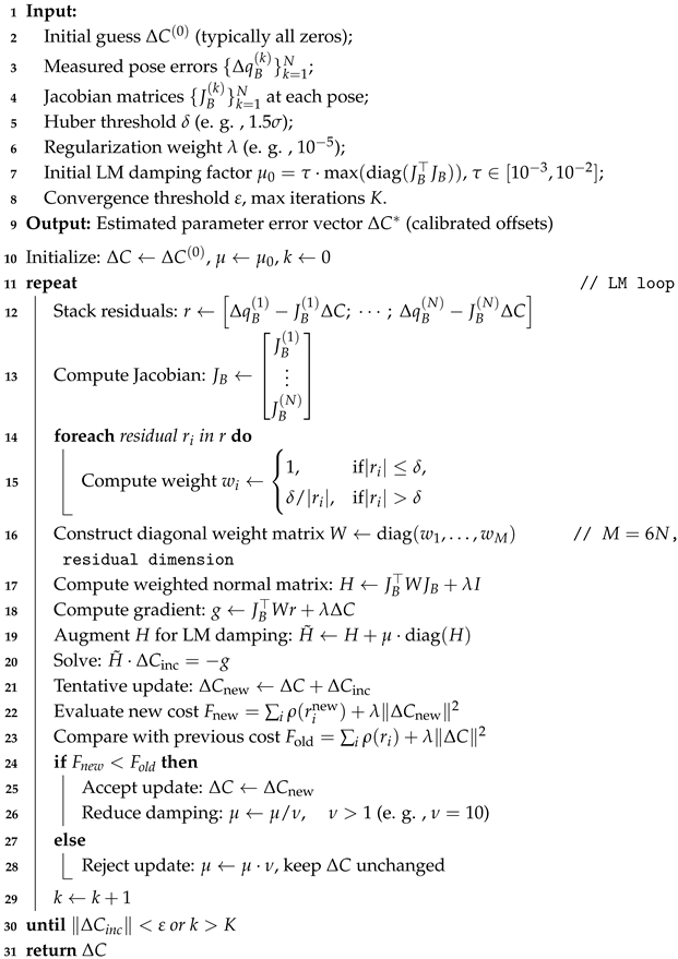
4.1. Simulation Verification

To validate the effectiveness of the proposed algorithm, a comprehensive simulation procedure was conducted, emulating the practical calibration scenario of the subreflector actuator. The simulation setup follows the theoretical framework described in Section 3, with synthetic pose errors generated using the linearized error model, additive Gaussian noise, and occasional outliers. The robust LM algorithm implements the Huber-weighted cost and L₂-regularized update rule exactly as specified, ensuring theory-consistent validation. In all simulation trials, both the traditional LM and the robust LM algorithms converged from the same initial conditions.

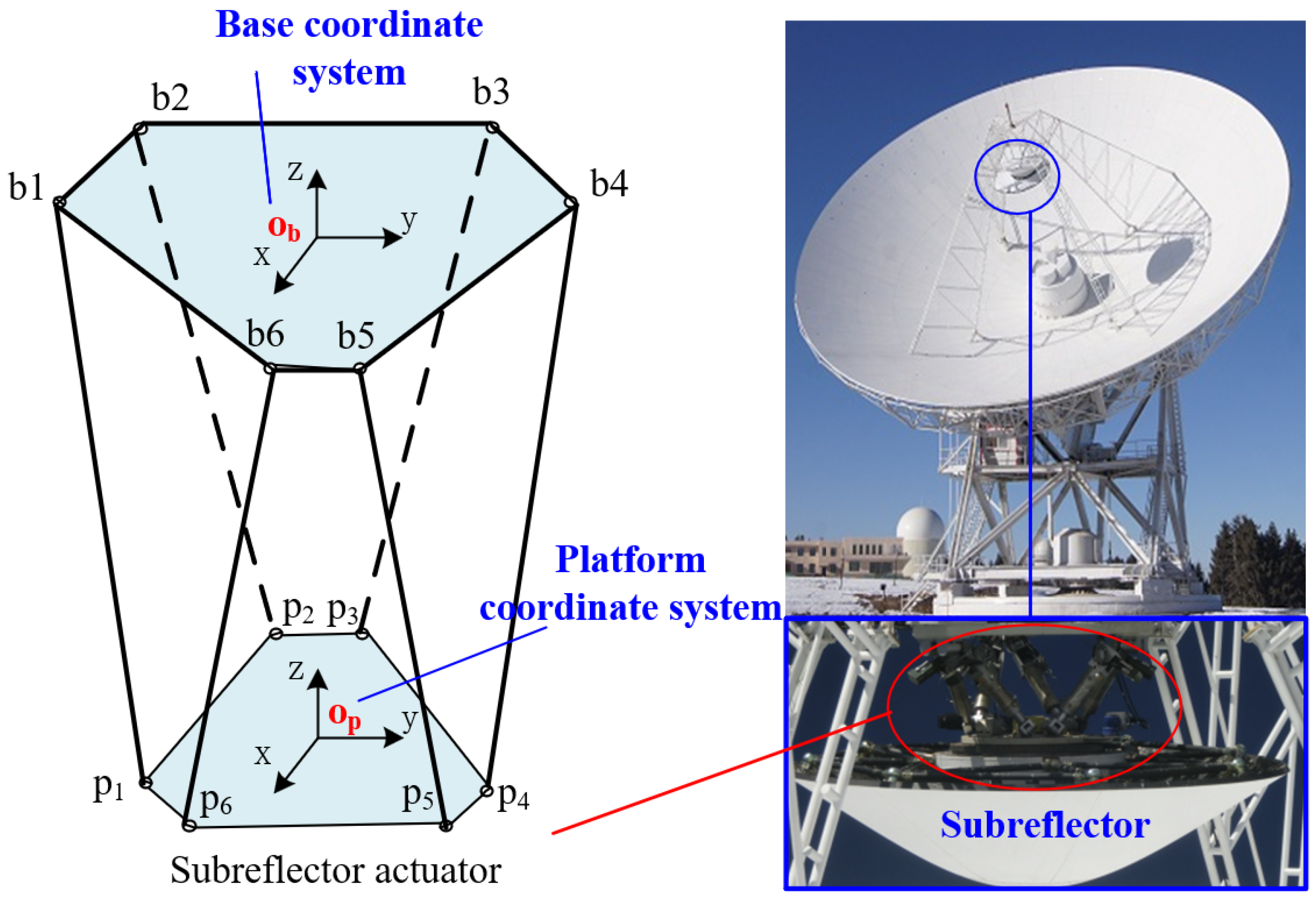
The geometric configuration and nominal kinematic parameters of the actuator are detailed in

Table 1. Kinematic parameters (unit: mm).

i	${\mathit{x}}_{\mathit{pi}}$	${\mathit{y}}_{\mathit{pi}}$	${\mathit{z}}_{\mathit{pi}}$	${\mathit{x}}_{\mathit{bi}}$	${\mathit{y}}_{\mathit{bi}}$	${\mathit{z}}_{\mathit{bi}}$	${\mathit{h}}_{\mathit{i}}$
1	242.6900	−60.0000	0	312.2660	−390.5000	0	564.1240
2	242.6900	60.0000	0	312.2660	390.5000	0	564.1240
3	−69.3850	240.0000	0	182.0500	465.6800	0	564.1240
4	−173.3080	180.1790	0	−494.3160	75.1800	0	564.1240
5	−173.3080	−180.1790	0	−494.3160	−75.1800	0	564.1240
6	−69.3850	−240.0000	0	182.0500	−465.6800	0	564.1240

, while the corresponding motion workspace bounds are defined in

Table 2. Workspace bounds (unit: mm and degree).

Axis	Lower Bound	Upper Bound
x	−50	50
y	−50	50
z	−50	50
Roll (°)	−5	5
Pitch (°)	−5	5
Yaw (°)	−5	5

. To ensure reliable identification of the 42 error components in the kinematic model, 50 poses within the reachable workspace were generated, and 30 additional poses were used for validation. Measurement poses are uniformly distributed within the portion of the subreflector actuator’s workspace that is visible to the external measurement system, using Latin Hypercube Sampling to ensure representative and space-filling coverage. This visibility-constrained region was used to avoid occlusion and maximize measurement quality. For each pose, the actuator’s forward kinematics is computed using the ground-truth parameters, after which controlled noise is injected to simulate sensor uncertainty and structural variability. The noise consists of a combination of white Gaussian noise and impulse noise.

Calibration was performed under four different workspace scales: 1, ${\displaystyle \frac{1}{2}}$, ${\displaystyle \frac{1}{5}}$, and ${\displaystyle \frac{1}{10}}$ of the whole reachable workspace.

Table 3. Comparison of position and orientation errors under different workspace scales.

Workspace Scale	Method	Position Error (mm)		Orientation Error (deg)
		Mean	Std	Mean	Std
$1\times$ Workspace	Traditional LM	0.1062	0.0475	0.0139	0.0061
	Robust LM	0.0329	0.0164	0.0034	0.0017
${\displaystyle \frac{1}{2}}\times$ Workspace	Traditional LM	0.1833	0.0799	0.0234	0.0114
	Robust LM	0.0596	0.0298	0.0059	0.0028
${\displaystyle \frac{1}{5}}\times$ Workspace	Traditional LM	0.3634	0.1635	0.0361	0.0194
	Robust LM	0.1276	0.0596	0.0122	0.0056
${\displaystyle \frac{1}{10}}\times$ Workspace	Traditional LM	0.4627	0.1830	0.0413	0.0217
	Robust LM	0.1905	0.0945	0.0194	0.0099

summarizes the simulation results under various workspace scales. As the workspace scale decreases, both position and orientation errors increase for both methods. However, the robust LM method produces significantly smaller errors compared to the traditional LM method, especially in the smaller workspace scales.

The standard deviation of the position and orientation errors increases substantially for traditional LM when moving to a ${\displaystyle \frac{1}{10}}\times$ workspace (from 0.0475 mm to 0.1830 mm in position, and from 0.0061° to 0.0217° in orientation). For the robust LM, these increases are far smaller (from 0.0164 mm to 0.0945 mm and 0.0017° to 0.0099°). This reflects the greater stability and repeatability of the robust method, suggesting it is less susceptible to “fluctuating fits” due to local minima or data inconsistency.

Smaller workspaces often lead to near-singular Jacobians. While LM handles this partially via damping, the robust LM further improves conditioning by modulating weight matrices dynamically and applying ridge regularization. This results in better-conditioned normal equations and explains why the robust LM converges more reliably. Traditional LM may either stagnate or produce unstable parameter updates in such cases, whereas the robust LM explicitly includes $L_2$ regularization, which acts as a prior to penalize large parameter magnitudes. This reduces overfitting tendencies, and explains why robust LM maintains better generalization across workspace scales.

Although the workspace shrinkage is the main source of accuracy degradation here, it effectively simulates scenarios where measurement noise or sensor bias dominate due to limited excitation. In such regimes, robust LM’s weighting mechanism naturally down-weights the influence of unstable directions in the residual space, behaving similarly to a noise filter. Traditional LM, in contrast, treats all residuals equally and is more prone to be skewed by small errors in low-excitation directions.

The calibration performance was further evaluated under varying levels of synthetic measurement noise to assess the robustness of the proposed algorithm at a $1\times$ workspace. Specifically, three representative noise levels were introduced to simulate real-world uncertainties in sensor readings and structural perturbations. Position noise was applied with a Gaussian distribution within the ranges of ±0.01 mm, ±0.05 mm, and ±0.1 mm, while the corresponding orientation noise was added with a Gaussian distribution within the ranges of ±0.001°, ±0.005°, and ±0.01°, respectively. Additionally, an impulse noise of 0.5 mm for position and 0.05° for orientation was added to each data set with a 5% probability.

Table 4. Comparison of position and orientation errors under different noise levels.

Noise Level	Method	Position Error (mm)		Orientation Error (deg)
		Mean	Std	Mean	Std
$\pm 0.01$ mm, $\pm 0.{001}^{\circ }$	Traditional LM	0.1253	0.0697	0.0126	0.0054
	Robust LM	0.0078	0.0034	0.0008	0.0004
$\pm 0.05$ mm, $\pm 0.{005}^{\circ }$	Traditional LM	0.3835	0.1389	0.0273	0.0079
	Robust LM	0.0973	0.0369	0.0076	0.0028
$\pm 0.1$ mm, $\pm 0.{01}^{\circ }$	Traditional LM	0.3985	0.1708	0.0279	0.0123
	Robust LM	0.1513	0.0722	0.0106	0.0053

presents a comparative evaluation of the calibration performance under varying levels of simulated measurement noise. Both the traditional LM and the proposed robust LM methods were tested across three noise levels, ranging from low to high, to emulate real-world measurement uncertainties in position and orientation.

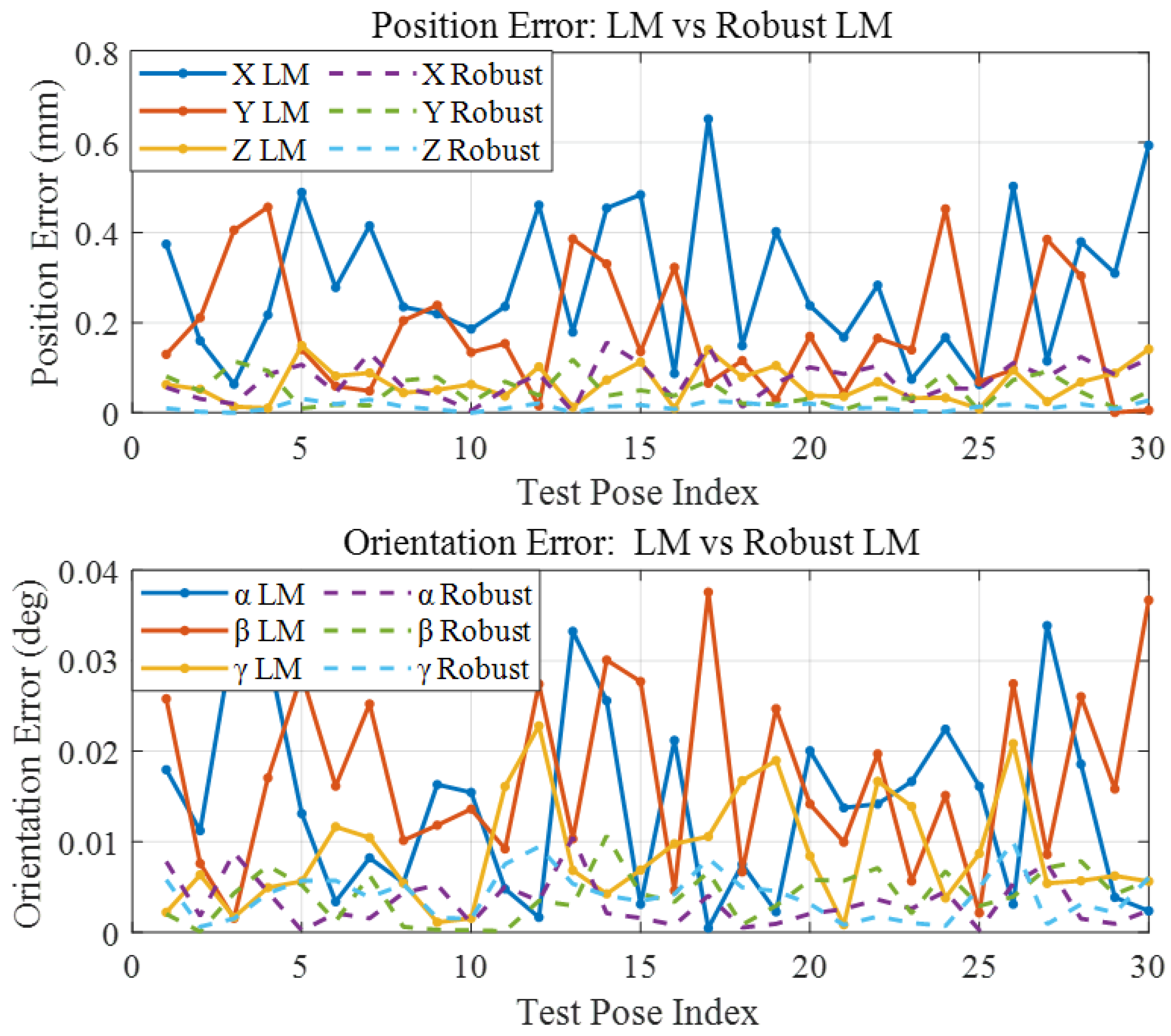
As shown in Figure 2, at the lowest noise level $[-0.01,0.01]\mathrm{mm}, {[-0.001,0.001]}^{\circ }$, the robust LM algorithm achieves exceptionally high accuracy, with a mean position error of only 0.0078 mm and a mean orientation error of 0.0008°. In comparison, the traditional LM records 0.1253 mm and 0.0126°, respectively. This translates to an improvement of approximately 93.8% in position accuracy and 93.7% in orientation accuracy, confirming the superior precision of the robust approach even in well-conditioned noise scenarios. Furthermore, the robust LM algorithm demonstrates a strong capability in effectively managing outliers, further enhancing its reliability in practical applications.

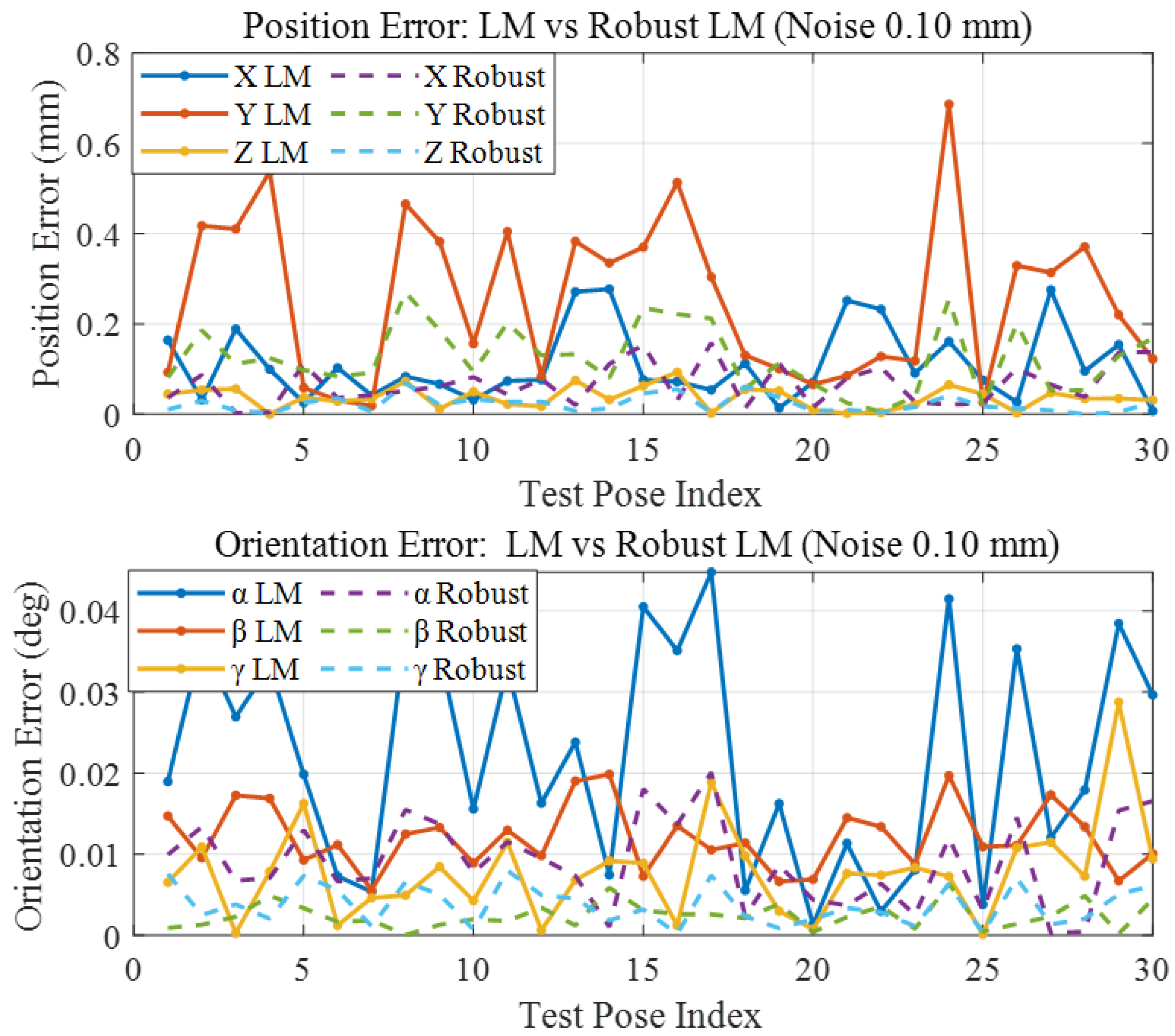
As shown in Figure 3, as noise levels increase to $[-0.05,0.05]\mathrm{mm}, {[-0.005,0.005]}^{\circ }$, the error gap between the two methods becomes even more evident. The position error for the traditional LM grows significantly to 0.3835 mm, while the robust LM maintains a much lower error of 0.0973 mm, reflecting a 74.6% reduction. Similarly, the orientation error is reduced from 0.0273° to 0.0076°, an improvement of 72.2%. These results highlight the noise suppression capability of the robust algorithm, particularly through the influence-limiting behavior of the Huber loss.

As shown in Figure 4, even under the most challenging condition tested (±0.1 mm noise, ±0.01° noise, and 5% outliers), the robust LM still converged and produced a mean residual positioning error of 0.1513 mm, while the traditional LM yielded 0.3985 mm. This corresponds to a deviation from the true parameters on the order of a few percent for the robust LM, compared to tens of percent for the traditional LM.

Traditional LM minimizes squared residuals, giving disproportionate influence to large errors, especially under high noise. In contrast, robust LM employs the Huber loss, which:

(1)

Weights small residuals quadratically for efficiency.

(2)

Weights large residuals linearly to limit their influence.

This allows robust LM to act as a soft outlier detector, down-weighting contaminated samples rather than letting them dominate the parameter update, which explains its better behavior at high noise.

As measurement noise increases, Jacobians derived from noisy data can become ill-conditioned, leading to unstable updates or even divergence in the traditional LM algorithm due to the absence of inherent regularization mechanisms. In contrast, the proposed robust LM approach incorporates $L_2$ regularization, which introduces numerical damping and significantly improves matrix conditioning. When combined with the adaptive weighting of the Huber loss function, this strategy ensures stable and reliable convergence, even in the presence of substantial noise and outlier contamination in the residuals. The additional weight updates and regularization terms introduce negligible computational overhead, and the robust algorithm’s convergence speed was similar to that of conventional LM in our tests, preserving near real-time performance. These findings underscore the robustness, adaptability, and strong generalization capability of the proposed method.

4.2. Experimental Results

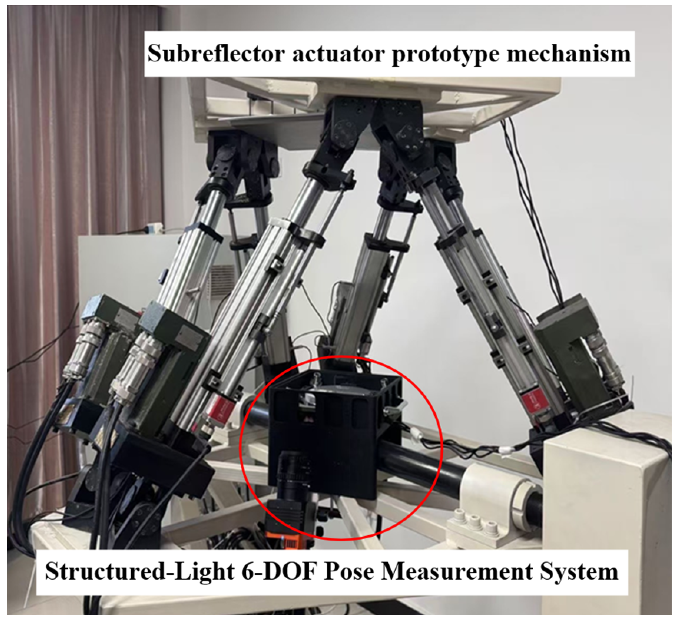
The subreflector actuator prototype mechanism and the structured-light 6-DOF pose a measurement system as shown in Figure 5. The system is composed of four 650 nm laser modules arranged in intersecting pairs, a mirror, a planar retroreflective target, and a camera. The laser projector mirror and camera were mounted on the base platform, while a planar retroreflective target was mounted rigidly on the movable platform. As the movable platform executed controlled translations or rotations, the laser spots moved on the target. The system projects a pre-calibrated pattern of laser spots onto a retro-reflective target attached to the subreflector and uses multiple high-resolution cameras to reconstruct the full 6-DOF pose. The effective measurement range of the system spans ± 30 mm along the x, y, and z axes, and ±4° in rotation about each of the x, y, and z axes. Repeated measurements under static conditions showed translational deviation RMS = 0.05 mm, while the angular error inferred from laser spot displacement remained below 0.001°.

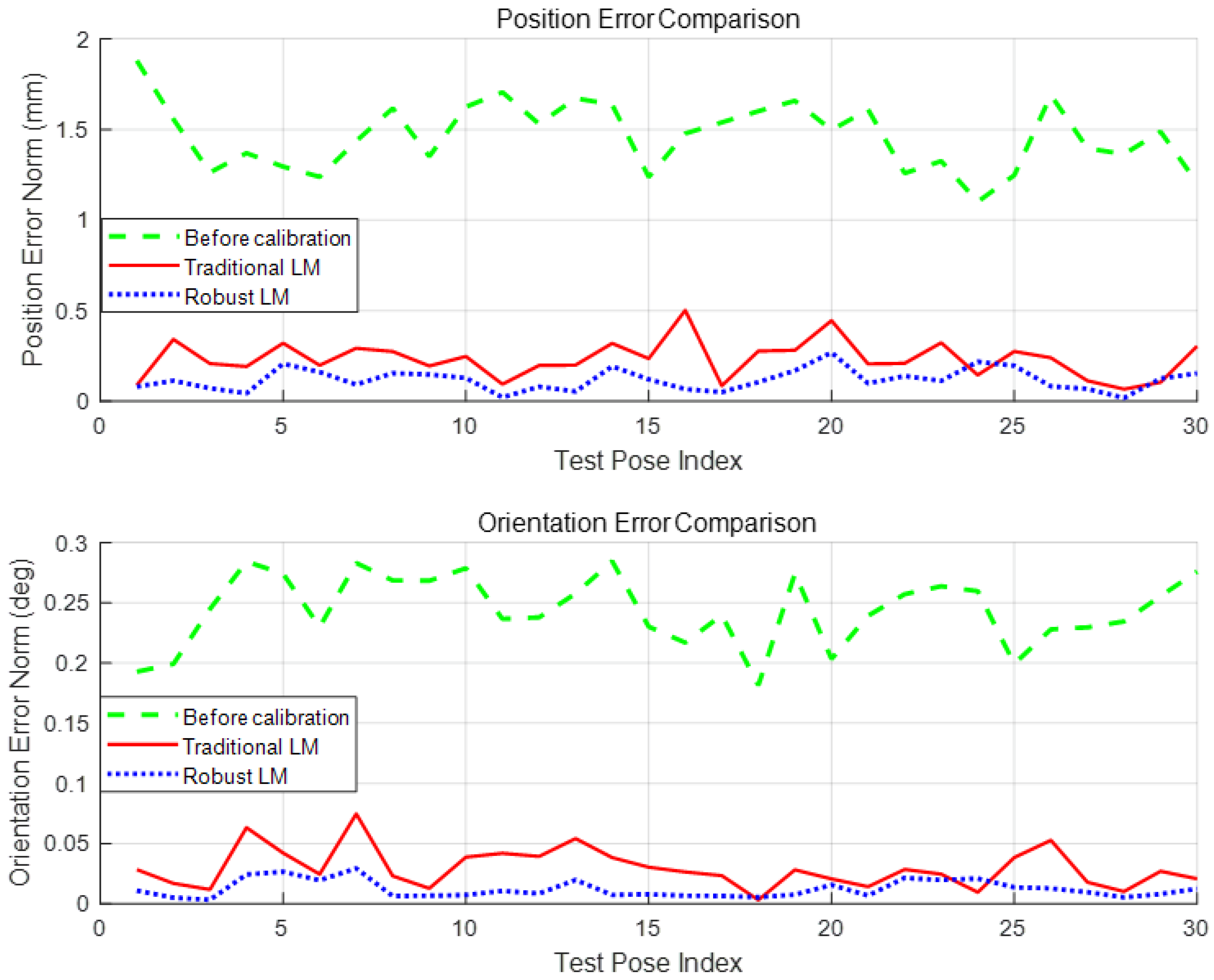
The kinematic calibration experiment was conducted based on a nominal set of measurement poses. The position and orientation errors before and after calibration are summarized in

Table 5. Comparison of position errors for different calibration methods.

Method	Mean (mm)	Std (mm)	Max (mm)
Before calibration	1.4626	0.1875	1.8804
Robust LM	0.1182	0.0608	0.2690
Traditional LM	0.2327	0.1027	0.5024

and

Table 6. Comparison of orientation errors for different calibration methods.

Method	Mean (°)	Std (°)	Max (°)
Before calibration	0.2444	0.0295	0.2847
Robust LM	0.0121	0.0072	0.0293
Traditional LM	0.0295	0.0165	0.0747

, and illustrated in Figure 6.

Prior to calibration, the mean position error was 1.4626 mm. After applying the robust LM algorithm, this was reduced to 0.1182 mm, representing a 91.9% improvement. In comparison, the traditional LM approach achieved a higher mean error of 0.2327 mm, nearly twice that of the robust method. The maximum position error decreased from 1.8804 mm to 0.2690 mm using robust LM, whereas traditional LM reduced it to 0.5024 mm.

For orientation, the mean error before calibration was 0.2444°. Robust LM reduced this to 0.0121°—a 95.0% reduction—while traditional LM converged to 0.0295°. Similarly, the maximum orientation error was reduced from 0.2847° to 0.0293° under the robust approach.

Overall, the robust LM algorithm consistently outperformed the traditional LM across all evaluated metrics. Its ability to suppress both positional and angular deviations, while maintaining low variance, makes it a highly reliable and accurate solution for high-precision 6-DOF calibration tasks under conditions of modeling uncertainty and measurement noise.

5. Discussion

The proposed robust LM algorithm, combining Huber loss and $L_2$ regularization, demonstrated notable improvements in calibration accuracy and stability under varying noise and workspace conditions. Compared to the traditional LM method, the robust version achieved significantly lower mean residual errors and exhibited enhanced resistance to outliers and ill-conditioning. While both methods successfully converged in simulations and experiments, the robust LM consistently delivered more reliable and accurate solutions, particularly in the presence of non-ideal measurements.

Nevertheless, we observed a discrepancy between simulation and experimental outcomes, even when the assumed noise magnitude was similar. This difference can be attributed to the following key factors:

(1)

Noise Distribution and Environmental Factors: In simulations, noise was modeled as ideal white Gaussian noise. In the experimental setup, a structured-light 6-DOF measurement system was used to obtain reference poses. To minimize systematic errors and long-term drift, the system was carefully calibrated before data collection, and all measurements were conducted under stable indoor conditions within a short time window. However, the system can still be affected by non-ideal factors such as low-frequency noise, surface reflection errors, or slight mounting shifts. These effects are difficult to model precisely and may introduce small biases into the data. These unmodeled deviations from ideal noise can result in broader residuals and reduced calibration precision.

(2)

Systematic and Modeling Errors: The simulation framework assumed a perfectly aligned measurement system and a rigid-body kinematic model. In contrast, the experimental setup may include residual biases in sensor calibration or target alignment, as well as structural non-idealities such as compliance, mounting clearance, or localized deformation. These systematic discrepancies are not fully captured by the error model and may lead to consistent deviations in the estimated parameters. While the robust LM can mitigate random errors and outliers, systematic mismatches between the model and hardware can still influence the final solution.

(3)

Limited Measurement Volume and Pose Coverage: The effective measurement region of the structured-light system imposed constraints on the range of feasible calibration poses. As a result, the experimental calibration covered a narrower portion of the actuator’s full workspace compared to simulation. This can lead to weaker excitation of certain parameters and a more ill-conditioned identification problem. Although our robust method remained stable under such reduced excitation, the overall error reduction was not as pronounced as in idealized simulations. The disparity in pose coverage and parameter observability partially explains the observed performance gap between simulation and experiment.

In summary, although the nominal noise levels are comparable, real-world calibration accuracy is inevitably affected by non-ideal noise distributions, correlated measurement errors, model inaccuracies, and limited pose coverage. These factors jointly contribute to larger residuals in experimental results compared to simulations. Nevertheless, the proposed robust LM algorithm consistently outperforms the traditional LM approach, delivering improved accuracy, robustness, and reliability. It is therefore particularly well-suited for the periodic calibration of subreflector actuators in already-deployed radio telescopes.

Despite its advantages, the robust LM method may still encounter challenges under extreme conditions, such as highly nonlinear error surfaces, poor initial parameter estimates, or correlated sensor faults, which may result in slower convergence or convergence to local minima. To address these limitations, future work will explore the integration of advanced data-driven compensation strategies to account for systematic biases and unmodeled dynamics. Such enhancements aim to enable adaptive, real-time correction across the full operational workspace, thereby expanding the method’s applicability to complex and variable real-world engineering systems.

6. Conclusions

This paper presents a robust kinematic calibration framework for subreflector actuators, integrating Huber loss and $L_2$ regularization into the LM optimization algorithm. A comprehensive simulation study was conducted, covering variations in workspace size and sensor noise conditions. The method demonstrated strong robustness under reduced pose excitation and high-noise scenarios, maintaining stable convergence where conventional methods showed degradation. These results confirm its effectiveness for high-precision 6-DOF calibration of parallel mechanisms, particularly in situations where full workspace excitation or ideal measurement conditions are not guaranteed.

Experimental validation using a structured-light 6-DOF measurement system further verified the method’s effectiveness. Compared to the conventional LM approach, the proposed method achieved over 90% reduction in both position and orientation errors, delivering repeatable and accurate parameter estimates. The integration of adaptive loss weighting and regularization effectively mitigates the influence of noise and outliers, enhancing convergence reliability in real-world scenarios. Consequently, the proposed method is particularly well-suited for the periodic calibration of subreflector actuators in operational radio telescopes, where measurement noise, limited pose excitation, and environmental disturbances are inevitable constraints. Moreover, this robust LM framework can be extended to other multi-degree-of-freedom systems in robotics, aerospace, and precision engineering, where calibration robustness and accuracy are equally critical.

References

1. Rohlfs, K.; Wilson, T.L. Tools of Radio Astronomy; Springer Science and Business Media: Berlin/Heidelberg, Germany, 2013; pp. 142–149. [Google Scholar]
2. Thompson, A.R.; Moran, J.M.; Swenson, G.W. Interferometry and Synthesis in Radio Astronomy; Springer: Berlin/Heidelberg, Germany, 2017. [Google Scholar]
3. Jáuregui, J.C.; Hernández, E.E.; Ceccarelli, M.; López-Cajún, C.; García, A. Kinematic Calibration of Precise 6-DOF Stewart Platform-Type Positioning Systems for Radio Telescope Applications. Front. Mech. Eng. 2013, 8, 252–260. [Google Scholar] [CrossRef]
4. Wang, N.; Xu, Q.; Ma, J.; Liu, Z.; Liu, Q.; Zhang, H.; Pei, X.; Chen, M.; Manchester, R.N.; Lee, K.; et al. The Qitai Radio Telescope. Sci. China Phys. Mech. Astron. 2023, 66, 289512. [Google Scholar] [CrossRef]
5. Xu, Q.; Li, L.; Cheng, A.Y. Preliminary Research on Connecting Strategy between Back-Up Structure and Alidade for 110-m Qitai Radio Telescope. Appl. Mech. Mater. 2015, 741, 61–65. [Google Scholar] [CrossRef]
6. Kazezkhan, G.; Xu, Q.; Wang, N.; Xue, F.; Wang, H. Performance Analysis and Optimization of a Modified Stewart Platform for the Qitai Radio Telescope. Res. Astron. Astrophys. 2023, 23, 095022. [Google Scholar] [CrossRef]
7. Prestage, R.M.; Constantikes, K.T.; Balser, D.S.; Condon, J.J. The GBT precision telescope control system. Proc. SPIE Ground-Based Telescopes 2004, 5489, 1029–1040. [Google Scholar] [CrossRef]
8. Pietzner, J.; Nothnagel, A. Deformation Effects of the Effelsberg 100 m Radio Telescope. EGU Gen. Assem. Conf. Abstr. 2010, 12, 11214. [Google Scholar]
9. Gawronski, W.; Souccar, K. Control Systems of the Large Millimeter Telescope. IEEE Antennas Propag. Mag. 2005, 47, 41–49. [Google Scholar] [CrossRef]
10. Wootten, A.; Thompson, A.R. The Atacama Large Millimeter/Submillimeter Array. Proc. IEEE 2009, 97, 1463–1471. [Google Scholar] [CrossRef]
11. Su, Y.X.; Duan, B.Y. The Application of the Stewart Platform in Large Spherical Radio Telescopes. J. Robot. Syst. 2000, 17, 375–383. [Google Scholar] [CrossRef]
12. Shen, Z.Q. Tianma 65-m Radio Telescope. In Proceedings of the 3rd China-US Workshop on Radio Astronomy Science and Technology-Emerging Opportunities, Green Bank, WV, USA, 19–21 May 2014. [Google Scholar]
13. Kazezkhan, G.; Xiang, B.; Wang, N.; Yusup, A. Dynamic Modeling of the Stewart Platform for the NanShan Radio Telescope. Adv. Mech. Eng. 2020, 12, 1687814020940072. [Google Scholar] [CrossRef]
14. Zhu, S.; Cheng, G.; Guo, F.; Pang, Y. Dynamic Modeling and Response Analysis of an Optical Machining Robot with Prismatic Joint Clearance. Appl. Sci. 2025, 15, 3197. [Google Scholar] [CrossRef]
15. Wan, Q.; Song, C.; Zhou, Y.; Tong, R.; Ma, S.; Liu, G. Modeling and analysis of the flap actuation system considering the nonlinear factors of EMA, joint clearance and flexibility. Aerospace 2024, 11, 440. [Google Scholar] [CrossRef]
16. Wang, Y.; Zhang, Y.; Li, X. A comprehensive study of the effect of thermal deformation on the dynamic characteristics of the high-speed spindle unit with various preload conditions. Precis. Eng. 2023, 80, 1. [Google Scholar] [CrossRef]
17. Petrič, T.; Žlajpah, L. Kinematic Model Calibration of a Collaborative Redundant Robot Using a Closed Kinematic Chain. Sci. Rep. 2023, 13, 17804. [Google Scholar] [CrossRef]
18. Karmakar, S.; Turner, C.J. A Literature Review on Stewart-Gough Platform Calibrations. J. Mech. Des. 2024, 146, 083302. [Google Scholar] [CrossRef]
19. Nubiola, A.; Bonev, I.A. Absolute Calibration of an ABB IRB 1600 Robot Using a Laser Tracker. Robot. Comput.-Integr. Manuf. 2013, 29, 236–245. [Google Scholar] [CrossRef]
20. Luo, X.; Li, Z.; Jin, L.; Li, S. A Regularization Ensemble Based on Levenberg-Marquardt Algorithm for Robot Calibration. In Robot Control and Calibration: Innovative Control Schemes and Calibration Algorithms; Springer Nature: Singapore, 2023; pp. 69–89. [Google Scholar]
21. Zhang, X.; Li, Y.; Chu, G. Comparison of Parallel Genetic Algorithm and Particle Swarm Optimization for Parameter Calibration in Hydrological Simulation. Data Intell. 2023, 5, 904–922. [Google Scholar] [CrossRef]
22. Huang, L.; Chen, M.; Zheng, S.; He, C.; Zhu, E.; Zhang, Y. Research on the Kinematic Calibration of the 3-PTT Parallel Mechanism. J. Mech. Sci. Technol. 2023, 37, 4311–4325. [Google Scholar] [CrossRef]
23. Nguyen, H.X.; Cao, H.Q.; Nguyen, T.T.; Tran, T.N.C.; Tran, H.N.; Jeon, J.W. Improving Robot Precision Positioning Using a Neural Network Based on Levenberg Marquardt–APSO Algorithm. IEEE Access 2021, 9, 75415–75425. [Google Scholar] [CrossRef]
24. Yu, D. Kinematic Parameter Identification for a Parallel Robot with an Improved Particle Swarm Optimization Algorithm. Appl. Sci. 2024, 14, 6557. [Google Scholar] [CrossRef]
25. Wang, Z.; Cao, B.; Xie, Z.; Ma, B.; Sun, K.; Liu, Y. Kinematic Calibration of a Space Manipulator Based on Visual Measurement System with Extended Kalman Filter. Machines 2023, 11, 409. [Google Scholar] [CrossRef]
26. Feng, A.; Zhou, Y.; Zhang, R.; Zhao, W.; Li, Z.; Zhu, M. A Novel Kinematic Calibration Method for Robot Based on the Levenberg-Marquardt and Improved Marine Predators Algorithm. Measurement 2025, 243, 116125. [Google Scholar] [CrossRef]
27. Sun, Y.; Fang, X. Robust Calibration of Computer Models Based on Huber Loss. J. Syst. Sci. Complex. 2023, 36, 1456–1475. [Google Scholar] [CrossRef]
28. Liu, F.; Gao, G.; Na, J.; Zhang, F. L2-Regularization-Based Kinematic Parameter Identification for Industrial Robots in Limited Measurement Space. Actuators 2025, 14, 144. [Google Scholar] [CrossRef]
Figure 1. Schematic diagram of the radio subreflector actuator.
Machines 13 00484 g001
Figure 2. Comparison of position and orientation errors under [ 0.01 , 0.01 ] mm ,   [ 0.001 , 0.001 ] noise.
Machines 13 00484 g002
Figure 3. Comparison of position and orientation errors under [ 0.05 , 0.05 ] mm ,   [ 0.005 , 0.005 ] noise.
Machines 13 00484 g003
Figure 4. Comparison of position and orientation errors under [ 0.1 , 0.1 ] mm ,   [ 0.01 , 0.01 ] noise.
Machines 13 00484 g004
Figure 5. The subreflector actuator prototype mechanism and the structured-light 6-DOF pose measurement system.
Machines 13 00484 g005
Figure 6. Comparison of errors before and after calibration.
Machines 13 00484 g006