
Data-Driven Digital Twin Framework for Predictive Maintenance of Smart Manufacturing Systems

 ,
,  and
and
Abstract
1. Introduction
2. Methods
2.1. Framework Development
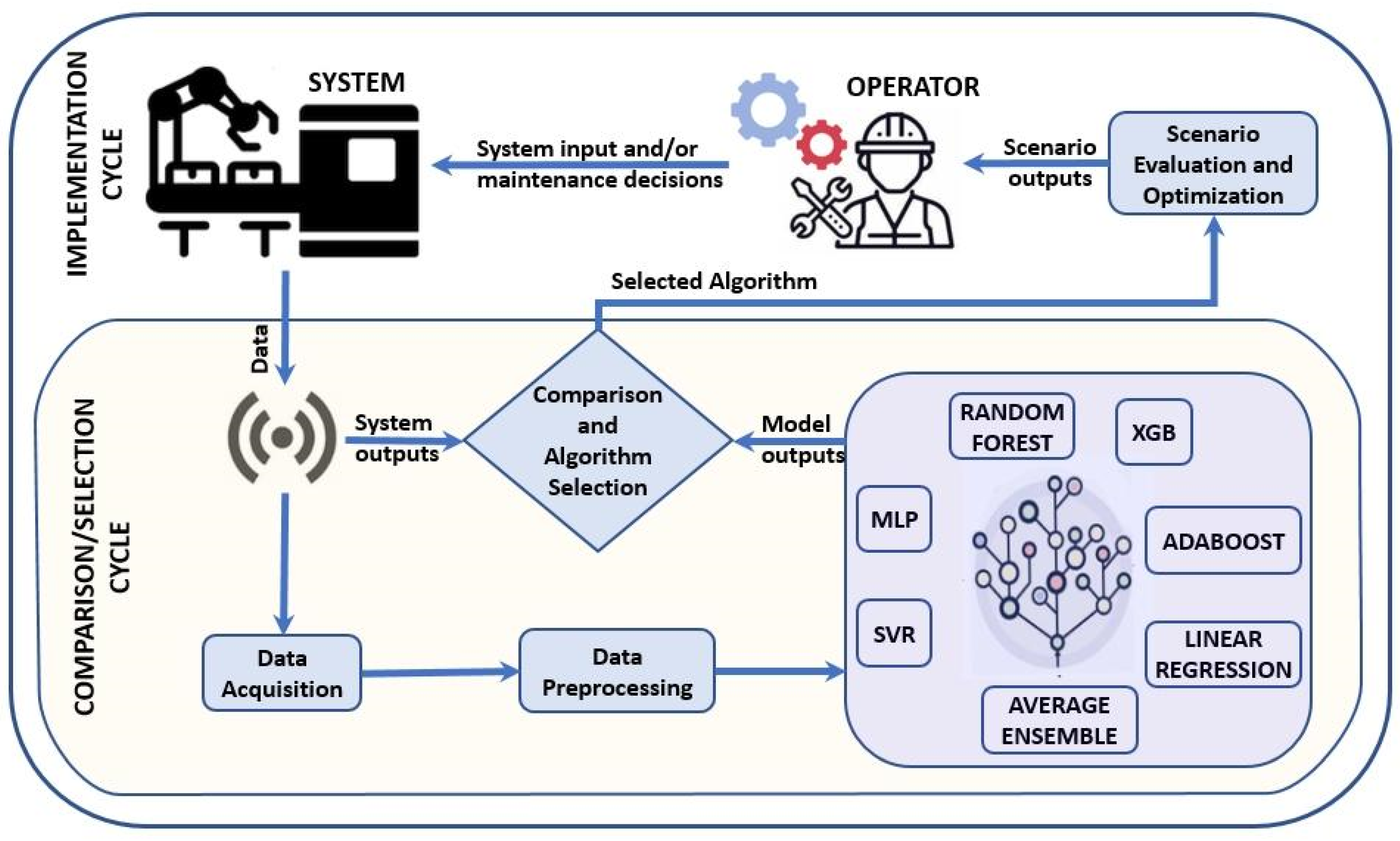
2.1.1. Maintenance System Architecture
2.1.2. Implementation of the Proposed System Architecture
2.1.3. Training and Testing of ML Models
2.2. Data-Driven Predictive Models
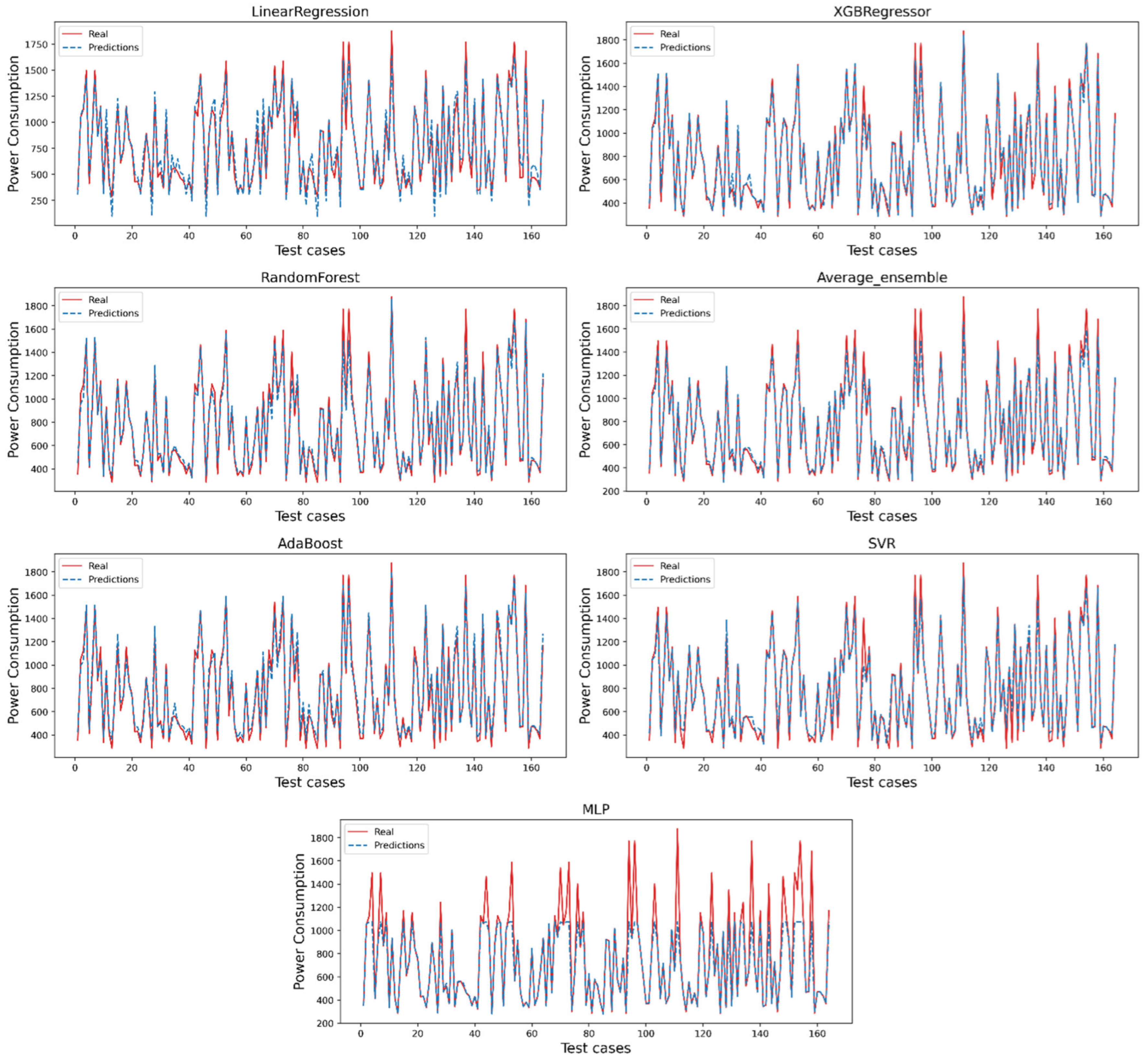
3. Results
4. Discussion
Author Contributions
Funding
Data Availability Statement
Acknowledgments
Conflicts of Interest
References
- Javaid, M.; Haleem, A.; Singh, R.P.; Suman, R.; Gonzalez, E.S. Understanding the adoption of Industry 4.0 technologies in improving environmental sustainability. Sustain. Oper. Comput. 2022, 3, 203–217. [Google Scholar] [CrossRef]
- Hulbert, S.; Mollan, C.; Pandey, V. Fault Diagnosis and Prediction in Automotive Systems with Real-Time Data Using Machine Learning. SAE Tech. Pap. 2022-01-0217 2022. [Google Scholar] [CrossRef]
- Slon, C.; Pandey, V.; Kassoumeh, S. Mixture distributions in autonomous decision-making for industry 4.0. SAE Int. J. Mater. Manuf. 2019, 12, 135–148. [Google Scholar] [CrossRef]
- SCOOP [Internet]. Tessenderlo, Limburg. 2022. Available online: https://www.i-scoop.eu/industry-4-0/ (accessed on 3 July 2024).
- Slon, C.; Pandey, V. Enabling autonomous decision-making in manufacturing systems through preference fusion. SAE Int. J. Mater. Manuf. 2020, 13, 109–124. [Google Scholar] [CrossRef]
- Monostori, L.; Kádár, B.; Bauernhansl, T.; Kondoh, S.; Kumara, S.; Reinhart, G.; Sauer, O.; Schuh, G.; Sihn, W.; Ueda, K. Cyber-physical systems in manufacturing. Cirp Ann. 2016, 65, 621–641. [Google Scholar] [CrossRef]
- Schmitt, R.; Permin, E.; Kerkhoff, J.; Plutz, M.; Böckmann, M.G. Enhancing resiliency in production facilities through cyber physical systems. Ind. Internet Things Cybermanuf. Syst. 2017, 287–313. [Google Scholar] [CrossRef]
- Khan, U.; Haleem, A. Smart organisations: Modelling of enablers using an integrated ISM and fuzzy-MICMAC approach. Int. J. Intell. Enterp. 2012, 1, 248–269. [Google Scholar] [CrossRef]
- Presciuttini, A.; Portioli-Staudacher, A. Applications of IoT and Advanced Analytics for manufacturing operations: A systematic literature review. Procedia Comput. Sci. 2024, 232, 327–336. [Google Scholar] [CrossRef]
- Khan, U.; Haleem, A. Improving to smart organization: An integrated ISM and fuzzy-MICMAC modelling of barriers. J. Manuf. Technol. Manag. 2015, 26, 807–829. [Google Scholar] [CrossRef]
- Canziani, A.; Paszke, A.; Culurciello, E. An analysis of deep neural network models for practical applications. arXiv 2016, arXiv:1605.07678. [Google Scholar] [CrossRef]
- Liu, C.; Jiang, P.; Jiang, W. Web-based digital twin modeling and remote control of cyber-physical production systems. Robot. Comput.-Integr. Manuf. 2020, 64, 101956. [Google Scholar] [CrossRef]
- Qamsane, Y.; Chen, C.Y.; Balta, E.C.; Kao, B.-C.; Mohan, S.; Moyne, J.; Tilbury, D.; Barton, K. A Unified Digital Twin Framework for Real-Time Monitoring and Evaluation of Smart Manufacturing Systems. In Proceedings of the 2019 IEEE 15th International Conference on Automation Science and Engineering (CASE), IEEE, Vancouver, BC, Canada, 22–26 August 2019; pp. 1394–1401. [Google Scholar] [CrossRef]
- Kessels, B.M.; Fey, R.H.; van de Wouw, N. Real-time parameter updating for nonlinear digital twins using inverse mapping models and transient-based features. Nonlinear Dyn. 2023, 111, 10255–10285. [Google Scholar] [CrossRef]
- Rojek, I.; Jasiulewicz-Kaczmarek, M.; Piechowski, M.; Mikołajewski, D. An artificial intelligence approach for improving maintenance to supervise machine failures and support their repair. Appl. Sci. 2023, 13, 4971. [Google Scholar] [CrossRef]
- Blume, C.; Blume, S.; Thiede, S.; Herrmann, C. Data-driven digital twins for technical building services operation in factories: A cooling tower case study. J. Manuf. Mater. Process. 2020, 4, 97. [Google Scholar] [CrossRef]
- Liu, D.; Du, Y.; Chai, W.; Lu, C.; Cong, M. Digital twin and data-driven quality prediction of complex die-casting manufacturing. IEEE Trans. Ind. Inform. 2022, 18, 8119–8128. [Google Scholar] [CrossRef]
- Akinsolu, M.O.; Zribi, K. A generalized framework for adopting regression-based predictive modeling in manufacturing environments. Inventions 2023, 8, 32. [Google Scholar] [CrossRef]
- Xu, Y.; Qamsane, Y.; Puchala, S.; Januszczak, A.; Tilbury, D.M.; Barton, K. A data-driven approach toward a machine-and system-level performance monitoring digital twin for production lines. Comput. Ind. 2024, 157, 104086. [Google Scholar] [CrossRef]
- Rathore, M.M.; Shah, S.A.; Shukla, D.; Bentafat, E.; Bakiras, S. The role of ai, machine learning, and big data in digital twinning: A systematic literature review, challenges, and opportunities. IEEE Access 2021, 9, 32030–32052. [Google Scholar] [CrossRef]
- Wang, P.; Luo, M. A digital twin-based big data virtual and real fusion learning reference framework supported by industrial internet towards smart manufacturing. J. Manuf. Syst. 2021, 58, 16–32. [Google Scholar] [CrossRef]
- Aivaliotis, P.; Georgoulias, K.; Chryssolouris, G. The use of Digital Twin for predictive maintenance in manufacturing. Int. J. Comput. Integr. Manuf. 2019, 32, 1067–1080. [Google Scholar] [CrossRef]
- Ho, S.L.; Xie, M.; Goh, T.N. A comparative study of neural network and Box-Jenkins ARIMA modeling in time series prediction. Comput. Ind. Eng. 2002, 42, 371–375. [Google Scholar] [CrossRef]
- Ran, Y.; Zhou, X.; Lin, P.; Wen, Y.; Deng, R. A Survey of Predictive Maintenance: Systems, Purposes and Approaches. arXiv 2019, arXiv:1912.07383. [Google Scholar] [CrossRef]
- Papacharalampopoulos, A.; Michail, C.K.; Stavropoulos, P. Manufacturing resilience and agility through processes digital twin: Design and testing applied in the LPBF case. Procedia Cirp 2021, 103, 164–169. [Google Scholar] [CrossRef]
- Khazraei, K.; Deuse, J. A strategic standpoint on maintenance taxonomy. J. Facil. Manag. 2011, 9, 96–113. [Google Scholar] [CrossRef]
- Yu, W.; Dillon, T.; Mostafa, F.; Rahayu, W.; Liu, Y. A global manufacturing big data ecosystem for fault detection in predictive maintenance. IEEE Trans. Ind. Inform. 2019, 16, 183–192. [Google Scholar] [CrossRef]
- Sakib, N.; Wuest, T. Challenges and opportunities of condition-based predictive maintenance: A review. Procedia Cirp 2018, 78, 267–272. [Google Scholar] [CrossRef]
- He, Y.; Gu, C.; Chen, Z.; Han, X. Integrated predictive maintenance strategy for manufacturing systems by combining quality control and mission reliability analysis. Int. J. Prod. Res. 2017, 55, 5841–5862. [Google Scholar] [CrossRef]
- Hosseinzadeh, A.; Chen, F.F.; Shahin, M.; Bouzary, H. A predictive maintenance approach in manufacturing systems via AI-based early failure detection. Manuf. Lett. 2023, 35, 1179–1186. [Google Scholar] [CrossRef]
- Garcia, M.C.; Sanz-Bobi, M.A.; Del Pico, J. SIMAP: Intelligent System for Predictive Maintenance: Application to the health condition monitoring of a windturbine gearbox. Comput. Ind. 2006, 57, 552–568. [Google Scholar] [CrossRef]
- Akhavei Bleicher, F. Predictive Modeling to Increase the Reliability of Production Planning in Single-Item Production. In Proceedings of the World Congress on Engineering and Computer Science 2016, San Francisco, CA, USA, 19–21 October 2016; Volume II, pp. 806–811. [Google Scholar]
- Lee, J.; Davari, H.; Singh, J.; Pandhare, V. Industrial Artificial Intelligence for industry 4.0-based manufacturing systems. Manuf. Lett. 2018, 18, 20–23. [Google Scholar] [CrossRef]
- Rahman, M.S.; Ghosh, T.; Aurna, N.F.; Kaiser, M.S.; Anannya, M.; Hosen, A.S. Machine learning and internet of things in industry 4.0: A review. Meas. Sens. 2023, 28, 100822. [Google Scholar] [CrossRef]
- De Simone, V.; Di Pasquale, V.; Miranda, S. An overview on the use of AI/ML in manufacturing MSMEs: Solved issues, limits, and challenges. Procedia Comput. Sci. 2023, 217, 1820–1829. [Google Scholar] [CrossRef]
- Canal, A.D.; Borille, A.V. CNC Turning: Roughness, Forces and Tool Wear [Dataset]. 2021 [Cited 2022]. In Kaggle [Internet]. [CrossRef]
- Plevris, V.; Solorzano, G.; Bakas, N.P.; Ben Seghier, M.E. Investigation of Performance Metrics in Regression Analysis and Machine Learning-Based Prediction Models. In Proceedings of the 8th European Congress on Computational Methods in Applied Sciences and Engineering (ECCOMAS Congress 2022), Oslo, Norway, 5–9 June 2022. [Google Scholar] [CrossRef]
- Mienye, I.D.; Sun, Y. A survey of ensemble learning: Concepts, algorithms, applications, and prospects. IEEE Access 2022, 10, 99129–99149. [Google Scholar] [CrossRef]
- Chicco, D.; Warrens, M.J.; Jurman, G. The coefficient of determination R-squared is more informative than SMAPE, MAE, MAPE, MSE and RMSE in regression analysis evaluation. Peerj Comput. Sci. 2021, 7, e623. [Google Scholar] [CrossRef]
- Willmott, C.J.; Matsuura, K. Advantages of the mean absolute error (MAE) over the root mean square error (RMSE) in assessing average model performance. Clim. Res. 2005, 30, 79–82. [Google Scholar] [CrossRef]
- Chai, T.; Draxler, R.R. Root mean square error (RMSE) or mean absolute error (MAE)?—Arguments against avoiding RMSE in the literature. Geosci. Model Dev. 2014, 7, 1247–1250. [Google Scholar] [CrossRef]
- Kim, S.; Kim, H. A new metric of absolute percentage error for intermittent demand forecasts. Int. J. Forecast. 2016, 32, 669–679. [Google Scholar] [CrossRef]
- Das, B.R.; Resnick, S.I. QQ plots, random sets and data from a heavy tailed distribution. Stoch. Models 2008, 24, 103–132. [Google Scholar] [CrossRef]


| Model | Tuning Method | Best Parameters |
|---|---|---|
| Linear Regression | Ridge Regression | {‘alpha’: 1, ‘fit_intercept’: True, ‘solver’: ‘auto’} |
| XGB Regressor | Randomized Search | {‘colsample_bytree’: 0.78, ‘gamma’: 0.007, ‘learning_rate’: 0.29, ‘max_depth’: 8, ‘n_estimators’: 341, ‘subsample’: 0.75} |
| Random Forest Regressor | Grid Search | {‘max_depth’: None, ‘max_features’: ‘log2’, ‘min_samples_leaf’: 1, ‘min_samples_split’: 5, ‘n_estimators’: 100} |
| AdaBoost Regressor | Grid Search | {‘estimator__max_depth’: 3, ‘learning_rate’: 1.0, ‘loss’: ‘square’, ’n_estimators’: 50 |
| SVR | Randomized Search | {‘C’: 1.03, ‘epsilon’: 0.105, ‘gamma’: ‘scale’, ‘kernel’: ‘rbf’ |
| MLP | Randomized Search | {‘activation’: ‘tanh’, ‘alpha’: 0.00208, ‘batch_size’: 128, ‘hidden_layer_sizes’: (50, 50), ‘learning_rate_init’: 0.0619} |
| Model | Tuning Method | Best Parameters |
|---|---|---|
| Linear Regression | Ridge Regression | {‘alpha’: 0.01, ‘fit_intercept’: True, ‘solver’: ‘svd’} |
| XGB Regressor | Randomized Search | {learning_rate = 0.29, max_depth = 8, n_estimators = 341, subsample = 0.75, colsample_bytree = 0.78, gamma = 0.007} |
| Random Forest Regressor | Grid Search | {‘estimator__max_depth’: 3, ‘learning_rate’: 1.0, ‘loss’: ‘square’, ‘n_estimators’: 200} |
| AdaBoost Regressor | Grid Search | {‘estimator__max_depth’: 3, ‘learning_rate’: 1.0, ‘loss’: ‘square’, ‘n_estimators’: 50} |
| SVR | Randomized Search | {‘C’: 98.96484985318548, ‘epsilon’: 0.03416347415306914, ‘gamma’: ‘auto’, ‘kernel’: ‘rbf’} |
| MLP | Randomized Search | {‘activation’: ‘logistic’, ‘alpha’: 0.010151348978007608, ‘batch_size’: 32, ‘hidden_layer_sizes’: (50, 50), ‘learning_rate_init’: 0.015226341829186325} |
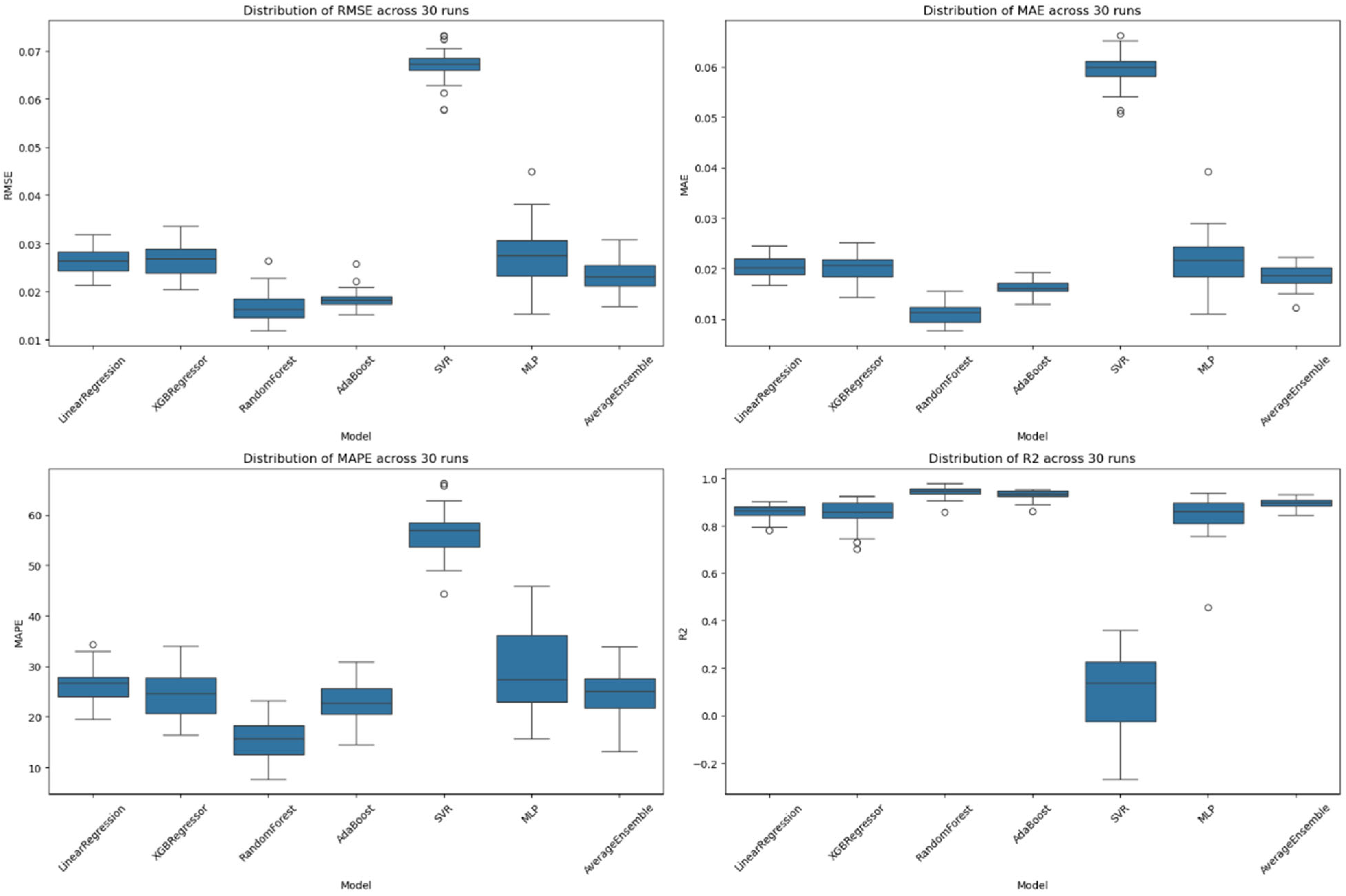
| ML Algorithm | MAPE | RMSE | ||
|---|---|---|---|---|
| Linear Regression | 0.020 ± 0.002 | 26.5% ± 3.4% | 0.027 ± 0.003 | 86.0% ± 2.8% |
| XGB Regressor | 0.020 ± 0.003 | 24.6% ± 4.8% | 0.027 ± 0.004 | 85.0% ± 5.3% |
| Random Forest Regressor | 0.011 ± 0.002 | 15.6% ± 4.0% | 0.017 ± 0.003 | 94.2% ± 2.4% |
| Average Ensemble | 0.016 ± 0.001 | 23.0% ± 3.8% | 0.018 ± 0.002 | 93.1% ± 2.1% |
| AdaBoost Regressor | 0.059 ± 0.003 | 56.2% ± 4.6% | 0.067 ± 0.004 | 9.7% ± 18.9% |
| SVR | 0.022 ± 0.005 | 29.4% ± 8.0% | 0.027 ± 0.006 | 84.5% ± 8.5% |
| MLP | 0.018 ± 0.002 | 24.7% ± 4.1% | 0.023 ± 0.003 | 89.4% ± 2.0% |
| Comparison | Z-Score | p-Value | Significant (p < 0.05) |
|---|---|---|---|
| Random Forest vs. Linear Regression | 12.0094 | 2.28606 × 10⁻¹⁷ | True |
| Random Forest vs. XGB Regressor | 8.25095 | 2.32836 × 10⁻¹¹ | True |
| Random Forest vs. Average Ensemble | 8.20355 | 2.7945 × 10⁻¹¹ | True |
| Random Forest vs. AdaBoost | 1.95375 | 0.055559 | False |
| Random Forest vs. SVR | 23.9245 | 9.76039 × 10⁻³² | True |
| Random Forest vs. MLP | 5.9513 | 1.63957 × 10⁻⁷ | True |
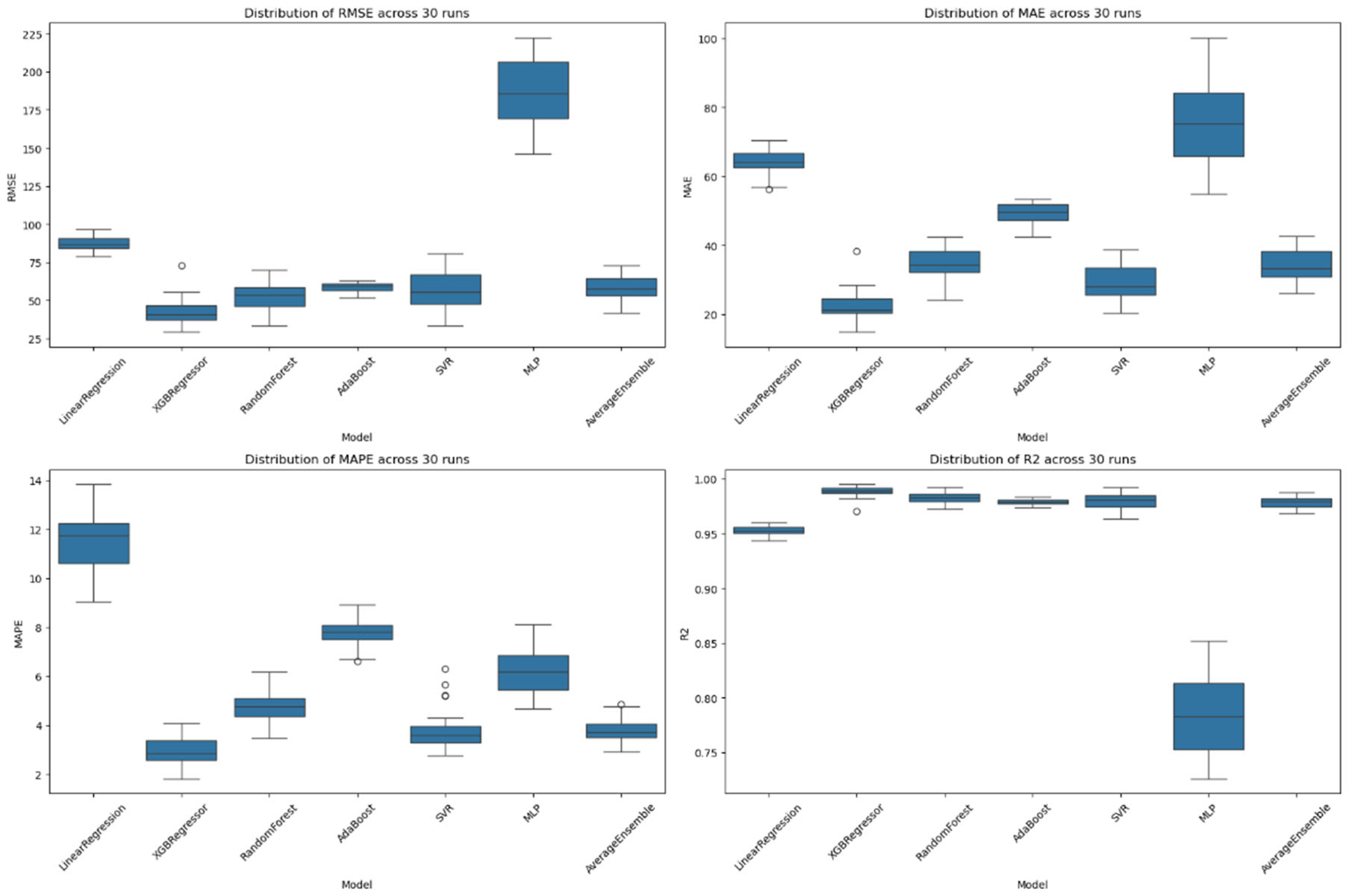
| ML Algorithm | MAPE | RMSE | |||
|---|---|---|---|---|---|
| Linear Regression | 64.076 ± 3.503 | 11.5% ± 1.2% | 87.650 ± 4.477 | 95.2% ± 0.4% | |
| XGB Regressor | 22.513 ± 4.424 | 3.0% ± 0.5% | 42.650 ± 8.933 | 98.9% ± 0.5% | |
| Random Forest Regressor | 34.959 ± 4.336 | 4.7% ± 0.6% | 52.650 ± 7.886 | 98.3% ± 0.5% | |
| Average Ensemble | 49.369 ± 3.001 | 7.8% ± 0.5% | 58.650 ± 3.119 | 97.9% ± 0.3% | |
| AdaBoost Regressor | 29.339 ± 4.861 | 3.8% ± 0.8% | 57.650 ± 11.564 | 97.9% ± 0.7% | |
| SVR | 75.970 ± 12.434 | 6.3% ± 1.0% | 186.650 ± 21.157 | 78.5% ± 3.5% | |
| MLP | 34.231 ± 4.613 | 3.8% ± 0.5% | 58.650 ± 8.667 | 97.8% ± 0.5% | |
| Comparison | Z-Score | p-Value | Significant (p < 0.05) |
|---|---|---|---|
| XGB Regressor vs. Linear Regression | 29.9667 | 5.46433 × 10−37 | True |
| XGB Regressor vs. Random Forest | 4.6573 | 1.914 × 10⁻⁵ | True |
| XGB Regressor vs. Average Ensemble | 8.20355 | 2.7945 × 10⁻¹¹ | True |
| XGB Regressor vs. AdaBoost | 7.78024 | 1.09453 × 10⁻¹³ | True |
| XGB Regressor vs. SVR | 5.63292 | 5.44446 × 10⁻⁷ | True |
| XGB Regressor vs. MLP | 31.2461 | 5.55743 × 10−38 | True |
Disclaimer/Publisher’s Note: The statements, opinions and data contained in all publications are solely those of the individual author(s) and contributor(s) and not of MDPI and/or the editor(s). MDPI and/or the editor(s) disclaim responsibility for any injury to people or property resulting from any ideas, methods, instructions or products referred to in the content. |
© 2025 by the authors. Licensee MDPI, Basel, Switzerland. This article is an open access article distributed under the terms and conditions of the Creative Commons Attribution (CC BY) license (https://creativecommons.org/licenses/by/4.0/).
Share and Cite
Khan, T.; Khan, U.; Khan, A.; Mollan, C.; Morkvenaite-Vilkonciene, I.; Pandey, V. Data-Driven Digital Twin Framework for Predictive Maintenance of Smart Manufacturing Systems. Machines 2025, 13, 481. https://doi.org/10.3390/machines13060481
Khan T, Khan U, Khan A, Mollan C, Morkvenaite-Vilkonciene I, Pandey V. Data-Driven Digital Twin Framework for Predictive Maintenance of Smart Manufacturing Systems. Machines. 2025; 13(6):481. https://doi.org/10.3390/machines13060481
Chicago/Turabian StyleKhan, Tarana, Urfi Khan, Adnan Khan, Calahan Mollan, Inga Morkvenaite-Vilkonciene, and Vijitashwa Pandey. 2025. "Data-Driven Digital Twin Framework for Predictive Maintenance of Smart Manufacturing Systems" Machines 13, no. 6: 481. https://doi.org/10.3390/machines13060481
APA StyleKhan, T., Khan, U., Khan, A., Mollan, C., Morkvenaite-Vilkonciene, I., & Pandey, V. (2025). Data-Driven Digital Twin Framework for Predictive Maintenance of Smart Manufacturing Systems. Machines, 13(6), 481. https://doi.org/10.3390/machines13060481