Abstract
Fault detection is a critical research area, especially in the automotive sector, aiming to quickly assess component conditions. Machine Learning techniques, powered by Artificial Intelligence, now represent state-of-the-art methods for this purpose. This study focuses on durability testing of Permanent Magnet Synchronous Motors for automotive applications, using Autoencoders (AEs) to predict and prevent failures. This AI-based fault detection strategy employs acceleration signals coming from electric motors tested under challenging conditions with significant variations in torque and speed. This approach goes beyond typical fault detection in steady-state conditions. Based on a review of Neural Networks, including Variational Autoencoders (VAEs), Convolutional Neural Networks (CNNs) and Long Short-Term Memory (LSTM) networks, the performance of six AI architectures is compared: AE, VAE, 1D CNN AE, 1D CNN VAE, LSTM AE and LSTM VAE. The 1D CNN AE outperformed the other networks in fault detection, showing high accuracy, stability and computational efficiency. The model is integrated into an algorithm for semi-real-time fault monitoring. The algorithm effectively detects potential motor failures in real-world scenarios, including bearing faults, mechanical misalignments, and progressive wear of components, thereby proactively preventing damage and halving test bench downtime.
1. Introduction
In recent years, electric vehicles (EVs) have emerged as a sustainable mobility solution, driven by technological advancements and the need to reduce emissions. Electric motors play a crucial role in this framework, impacting the performance, energy efficiency, and reliability of EVs. Ensuring their proper functioning is essential, making fault detection a key factor in maintaining consistent and efficient operation. Fault detection is the process of identifying malfunctions in a system to ensure performance and reliability. It involves monitoring, detecting anomalies and taking corrective actions to prevent damage. Effective fault detection reduces downtime, lowers maintenance costs and improves efficiency. Over the years, fault detection in industrial systems has significantly evolved, driven by advancements in technology. Initially, fault detection systems relied on basic condition monitoring techniques, which often failed to provide accurate and reliable diagnoses of mechanical failures. However, as industrial systems became more complex, the need for more sophisticated methods led to the adoption of “predictive maintenance” (PdM), which focuses on using data to optimise maintenance schedules [1], and “prognostics and health management” (PHM) [2], which aims to assess machine health and predict failures in advance. The integration of Big Data, the Internet of Things (IoT) and Artificial Intelligence (AI) [3] has revolutionised fault detection, enabling more comprehensive analysis through vast datasets gathered from connected devices across entire industrial systems [4]. Machine Learning (ML) and Deep Learning (DL) have further enhanced these methods by automatically extracting features and patterns from historical data, leading to more accurate and intelligent fault predictions. As a result, industries can now monitor systems in real time, significantly improving operational efficiency [4,5].
A crucial aspect of fault detection is that condition monitoring is an expert-driven task, with human intervention often being ineffective, particularly when dealing with large volumes of data. Therefore, intelligent condition monitoring techniques are essential to reduce human dependency. Among various AI-based methods, the Autoencoder (AE) has emerged as one of the most prominent ML approaches [6]. This is due to its unsupervised nature, which allows us to process large volumes of unlabelled data, without prior knowledge of what constitutes a faulty system. Autoencoders have gained significant attraction in the industry also thanks to their capability to analyse minimally preprocessed multi-variable datasets, enhancing fault detection in comparison to traditional methods, which typically rely on single-metric monitoring. Additionally, the architecture of the AE can be strengthened by incorporating other types of Neural Networks (such as CNNs or LSTMs), further improving its adaptability and making it a versatile tool for a wide range of applications.
Several studies have explored DL models, particularly Autoencoders, to analyse time signals in industrial systems and detect anomalies. Chen et al. [7] proposed a 1D CNN AE for fault detection and diagnosis in multivariate systems, incorporating a softmax layer for classification. Their supervised approach achieves high accuracy, even with noise, but relies on labelled fault data. Lee et al. [8] introduced a deep 1D CNN AE with a fully connected latent space for unsupervised fault detection in industrial gas turbines, using IQR (interquartile range)-based preprocessing to filter anomalies and evaluating performance via Mean Square Error (MSE). Ahmad et al. [9] developed an LSTM AE for early fault detection in rotating machinery, demonstrating superior feature extraction capabilities and generalisation across multiple machines, though requiring a large dataset for effective training. Wu et al. [10] introduced a DL framework that uses raw vibration inputs to construct health indicators via a convolutional Autoencoder. It effectively captures bearing wear and degradation trends, enabling early fault detection in rolling bearings. Eren et al. [11] demonstrated that 1D CNNs excel in bearing health monitoring by directly processing raw time-domain vibration data with minimal preprocessing, achieving high accuracy in fault detection compared to traditional frequency-based methods.
Regarding fault detection in electric motors, traditional approaches rely on monitoring individual indicators (e.g., vibration, voltage, current) and defining specific metrics, often involving complex processes. These techniques, generally classified into signal-based and model-based methods [12], are effective but require an in-depth understanding of the system, which makes their implementation challenging. Thanks to advances in AI, fault detection no longer relies on extensive domain knowledge, enabling a faster process. AI has been shown to significantly enhance fault detection and classification, ultimately leading to optimised performance and efficiency in electric motors [13]. Among all electric motor studies, Bae et al. [14] highlight the importance of fault prediction in electric motors to prevent production disruptions and additional costs. A multi-input Convolutional Neural Network (CNN) combined with image transformation techniques is proposed, achieving excellent classification performance and demonstrating its superiority over traditional methods. Principi et al. [15] compared different NN architectures for anomaly detection in DC motors using acceleration signals. Their results show that MLP (Multilayer Perceptron)-based AEs were the most effective, followed by LSTM AEs, while CNN AEs and OC-SVM (One-Class Support Vector Machine) perform worse. This study inspired the present research, extending the comparison by including VAE variants to all the AE proposed. Huang et al. [16] focused on optimising dimensionality reduction and fault detection accuracy, introducing a Recurrent Neural Network (RNN) VAE for acceleration signal analysis. Their study showed that GRU (Gated Recurrent Unit)-based models achieve up to 99% accuracy but require extensive training data, making real-time applications challenging.
Other research efforts have instead concentrated on real-time monitoring of electric motors, with the goal of ensuring reliable operation both during testing and under actual working conditions. Givnan et al. [17] proposed a Reduced Stacked Autoencoder (RSAE) for real-time fault detection in industrial motors, which offers lower computational effort and improved anomaly recognition. Their study introduce a “traffic light” threshold system to classify motor conditions dynamically. Ince et al. [18] focused on efficient feature extraction for real-time applications using a 1D CNN, relying exclusively on current signals from induction motors. Their method outperformed traditional classifiers and achieved a response time of under 1 ms. Similarly, Afrasiabi et al. [19] also focused on induction motors, evaluating an accelerated-CNN approach specifically for bearing fault detection. Their CNN-based method shows promising results compared to traditional techniques such as SVM and standard ANN models. An et al. [20] addressed the limitations of traditional approaches to real-time motor fault diagnosis by proposing an improved CNN model combined with an edge computing solution. The proposed CNN was optimised to reduce both model size and the number of parameters, achieving higher accuracy than classical Backpropagation Neural Networks. However, the fault diagnosis was conducted on a motor operating under stationary conditions with low power output, which reduced the complexity of the faults being analysed.
Contributions
The aim of this research is to identify the most effective AI-based method to perform fault detection in automotive Permanent Magnet Synchronous Motors (PMSMs) during endurance tests. The choice to focus solely on deep unsupervised learning techniques is supported by multiple recent works [15,21,22,23], which report that these approaches outperform traditional supervised models such as SVMs, Random Forests, supervised MLP networks and k-Nearest Neighbors (kNN) in comparable scenarios. In particular, AEs have been widely exploited for fault detection applications, showing strong potential alongside other DL techniques. This work addresses a gap in the literature by focusing on the application of AEs to electric motors under heavy load cycling conditions, characterised by highly variable speed and torque. In contrast, most existing studies focus on steady-state operating conditions [15,16]. These scenarios present a major challenge for AI-based methods due to the high variability of the dataset and the need to train with minimal amount of data. This constraint arises from the long testing cycles, making data collection costly and time-consuming.
In this paper, six different AE architectures are defined, inspired by the work of Principi et al. [15]: the standard Autoencoder (AE), the Variational Autoencoder (VAE), the 1-Dimensional Convolutional Neural Network Autoencoder (1D CNN AE), the 1-Dimensional Convolutional Neural Network Variational Autoencoder (1D CNN VAE), the Long Short-Term Memory Autoencoder (LSTM AE) and the Long Short-Term Memory Variational Autoencoder (LSTM VAE). These AEs exploit PMSMs vibration signals associated to mechanical orders, bearing orders and the vibration amplitude in the 10–1500 Hz frequency band as input data. Then, these networks are compared to identify the most robust, reliable and efficient model in predicting damages and ensuring that the motor is stopped before failure occurs, thereby improving monitoring efficiency and time/cost saving. Since the proposed algorithm is based on Machine Learning techniques, it is capable of identifying subtle patterns in operational data, thereby enabling the detection of various mechanical faults and control-related anomalies. In particular, the fault detection strategy has been validated on multiple fault types, including bearing faults and mechanical misalignments resulting from improper shaft connection. The outcome of this research will be a comprehensive fault detection algorithm utilising the selected AE architecture to monitor the condition of PMSMs under heavy-duty durability testing.
This paper is structured as follows: Section 2 presents the theoretical background on Neural Networks and Autoencoders, including VAE, CNN and LSTM. Section 3 describes the case study and the proposed fault detection method, while Section 4 reports the results obtained for fault detection using the AEs and discusses them. Finally, Section 5 provides the concluding remarks.
2. Artificial Intelligence Methods
Deep Learning is a subset of Machine Learning that uses Artificial Neural Networks (ANNs) to learn data representations hierarchically, enabling it to directly understand and extract features. Unlike traditional ML methods, DL automates feature extraction, making it particularly effective in handling raw data [3].
ANNs mimic the signal processing mechanisms of the human brain. The fundamental unit of ANNs is the neuron, which performs a weighted sum of inputs and passes it through an activation function. Neurons are organised into layers, with each layer learning hidden features from the previous one. The deepest layers extract more complex features [24]. Training plays a fundamental role in NNs, enabling the model to learn meaningful patterns and relationships within the data by iteratively adjusting its parameters. The objective is to develop a model that generalises effectively to unseen data. To do so, the training process utilises two datasets: the training set, which is used to update the model’s weights via the backpropagation algorithm, minimising the loss function; and the validation set, which is used to monitor performance and detect overfitting [25]. However, the training data varies depending on whether the ANN model follows a supervised or unsupervised learning approach. In supervised learning, the model is trained on labelled data to predict specific outputs, such as in classification or regression tasks. In contrast, unsupervised learning models work with unlabelled data to identify hidden patterns or structures, such as clustering or dimensionality reduction. Autoencoders (AEs) are a key example of unsupervised learning techniques used for anomaly detection [24].
2.1. Autoencoder Structure
This section presents the standard architectures of AEs and VAEs. In their basic form, both the encoder and decoder layers consist of standard neurons. In the following sections, the alternative architectures based on CNN and LSTM cells will be introduced.
2.1.1. Autoencoder
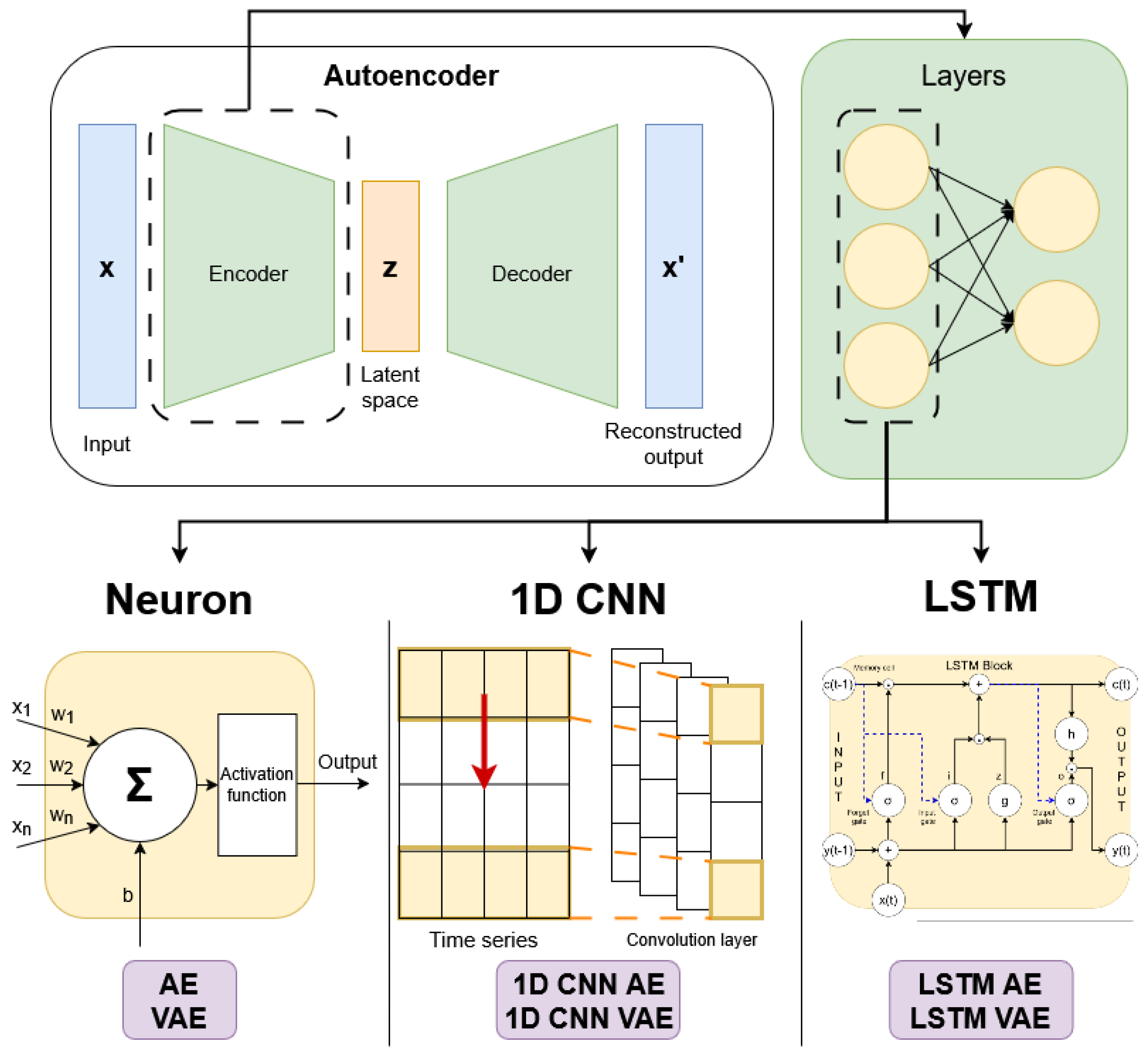
The key idea of Autoencoders is to reconstruct input data by extracting its most relevant features. To do so, AEs are divided into two parts: the encoder, which maps input data to a lower-dimensional feature space, and the decoder, which reconstructs the input from this latent representation [24]. This makes them effective for fault detection, as they can accurately reconstruct normal signals while struggling with anomalous ones, producing a high reconstruction error [6,24,26]. AEs reduce the number of neurons in each encoder layer, creating a bottleneck, represented by the latent space, that forces the network to learn essential features and accomplishing dimensionality reduction. Then, the decoder mirrors the encoder, as shown in the architecture presented in Figure 1.

Figure 1.
Autoencoder structure: The encoder and decoder consist of layers, defined in three ways: AE/VAE (dense networks), 1D CNN AE/VAE (convolutional layers for sequential data) and LSTM AE/VAE (recurrent networks for temporal data).
Mathematically, the encoding and decoding processes involve weight matrices, biases and activation functions such as ReLU, Tanh or sigmoid, which allow AEs to capture non-linear patterns, an advantage over methods like PCA (Principal Component Analysis) that only extract linear relationships [27]. Assuming both a single-layer encoder and decoder, the operations carried out by the Autoencoder can be described as follows [24]:
where z indicates the output of the encoder; and denote the weight and bias of the encoder function, respectively; and and , instead, are the weight and bias related to the decoder function. and represent the activation function of the encoder and decoder, respectively. The reconstruction function combines these operations, and training minimises the reconstruction error, usually measured by MSE.
2.1.2. Variational Autoencoder
Unlike standard AEs, the features extracted by VAEs are represented by a specific form of probability distribution, and the optimisation computation is based on the principles of variational Bayes inference [24]. This process enables the encoder to efficiently approximate the posterior distribution of the latent variables for all data points, improving computational performance during training [28]. In VAEs, the encoder learns the posterior distribution , which represents the probability of the latent variable z given the observed data x. The decoder models the likelihood , which describes how likely the data x is given a latent variable z. The encoder produces the mean and the standard deviation of the posterior distribution, which are used to sample z via the following reparametrisation trick:
This trick allows gradients to flow through the sampling process, enabling backpropagation during training. Instead, the prior distribution is usually assumed to be a standard Gaussian (), reflecting the assumption that the latent variables z are drawn from a simple, isotropic distribution before any data is observed.
The VAE is trained by maximising the Evidence Lower Bound (ELBO) [24,26]:
This formula consists of two terms: the first measures the decoder reconstruction error, which ensures that the VAE is able to reconstruct the output starting from the latent representation z, while the second (Kullback–Leibler divergence) regularises the latent space by minimising the difference between the posterior and the prior . This helps prevent the latent space from becoming too complex.
This whole formulation allows VAEs to generate new samples while maintaining structured latent representations, making them highly effective for unsupervised learning tasks.
2.2. Encoder–Decoder Cells
In the AE architecture, the encoder and the decoder are typically composed of standard neuron-based layers. However, in this case, they have also been designed using CNNs and LSTM networks, as depicted in Figure 1.
2.2.1. Convolutional Neural Network
Initially designed for 2D image processing, standard CNNs require reshaping 1D signals into 2D formats when applied to time-series data, as suggested by Janssens et al. [29]. However, this approach has significant drawbacks: deep CNNs demand substantial computational power and large datasets, making them unsuitable for real-time applications on low-end devices or in scenarios with limited labelled data. To overcome these limitations, 1D Convolutional Neural Networks (1D CNNs) were developed. Unlike traditional CNNs, 1D CNNs process time-series data directly, eliminating the need for reshaping and significantly reducing computational costs while preserving the core benefits of convolutional architectures and utilising the backpropagation algorithm for training [30]. A typical 1D CNN consists of the following:
- A 1D convolution operation, where filters extract patterns directly from sequential data.
- An activation function, usually ReLU, to improve stability and training efficiency [25].
- A sub-sampling operation (stride), which reduces dimensionality and prepares the data for the following layer.
Thanks to their efficiency and adaptability, 1D CNNs have become a widely used approach for time-series analysis, especially in applications with limited labelled data and highly variable signals from diverse sources. Their ability to perform parallel computations makes them ideal for real-time processing and resource-constrained environments [18].
2.2.2. Long Short-Term Memory
LSTMs are a special type of Recurrent Neural Network (RNN) designed to handle sequential data by maintaining long-term dependencies [31]. RNNs process sequences by transmitting information cyclically, enabling them to consider both current and past inputs. Their training relies on the Backpropagation Through Time (BPTT) algorithm [32], an extension of standard backpropagation that unfolds the network over time. However, RNNs face significant challenges due to the vanishing and exploding gradient problem, which can severely degrade training performance [32]. To address this limitation, LSTMs incorporate a set of gates to regulate information flow, enabling more stable and efficient learning [33]. These mechanisms make LSTMs particularly effective for sequential data processing, including time-series prediction, speech recognition and natural language processing [3].
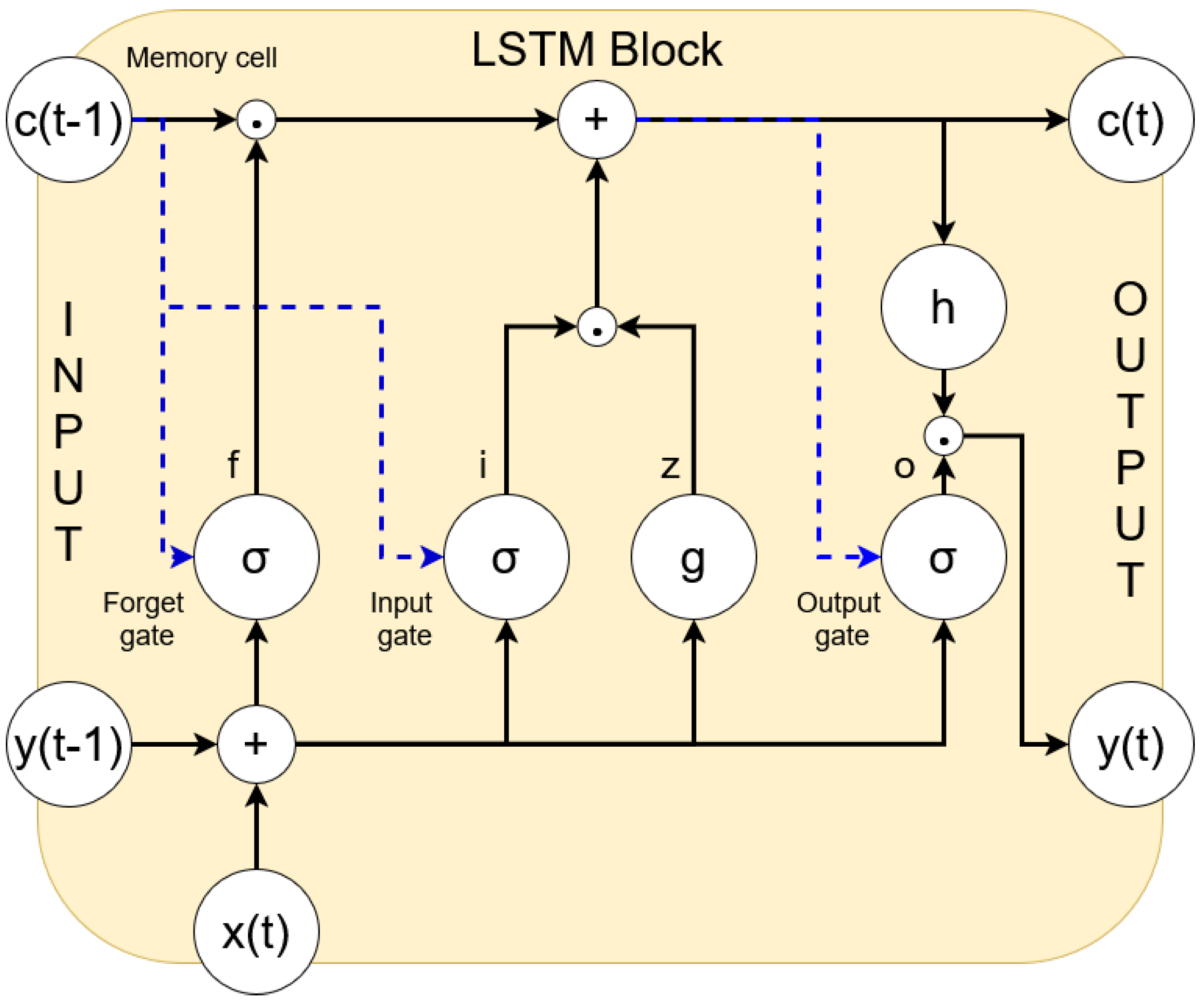
Each LSTM memory block, as depicted in Figure 2, consists of the following:
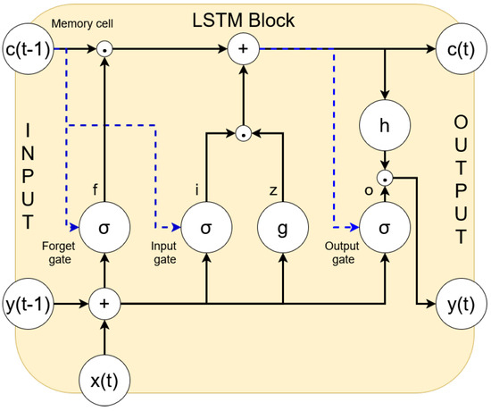
Figure 2.
Typical architecture of an LSTM block.
- A memory cell, which maintains its state over time.
- An input gate, which controls what new information should be added.
- A forget gate, which resets the memory when necessary.
- An output gate, which determines what part of the memory should be output.
Referring to Figure 2, the LSTM forward pass follows these steps:
- Block input update: It combines the current input x(t) and the previous output y(t − 1) to compute z(t).
- Input gate update: It uses x(t), y(t − 1), and the previous cell state c(t − 1) to compute i(t).
- Forget gate update: It determines which past information should be discarded.
- Cell state update: It combines the block input, input gate and forget gate to compute c(t).
- Output gate update: It computes o(t) based on current and past inputs.
- Final block output: The output y(t) is determined by the current cell state and the output gate.
The activation functions used are the sigmoid function , which controls the gate activations, and the hyperbolic tangent , which is used for input and output transformations [31].
3. Fault Detection Method
This section presents the proposed AI-based method for fault detection in electric motors. It is based on Autoencoders that exploit accelerometer signals measured at PMSMs subjected to duration cycles. In order to identify the best-performing AE for this problem, 6 different architectures are tested and compared: AE, VAE, 1D CNN AE, 1D CNN VAE, LSTM AE and LSTM VAE.
3.1. Testing Configuration
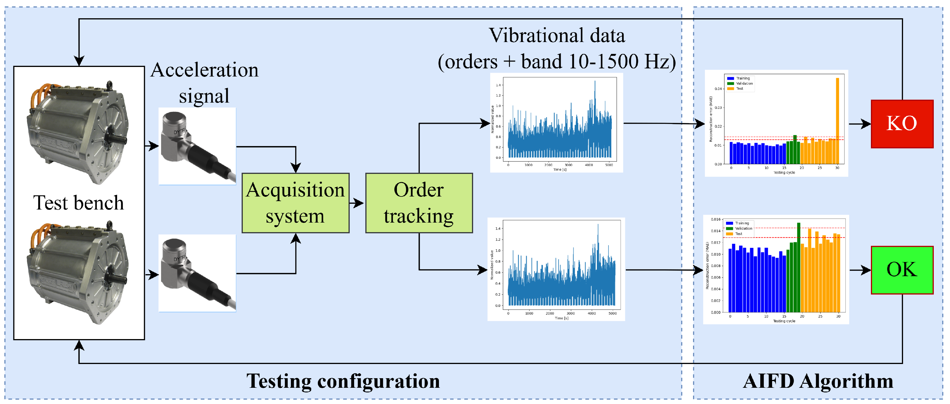
A schematic overview of the electric motor testing configuration is shown in Figure 3.
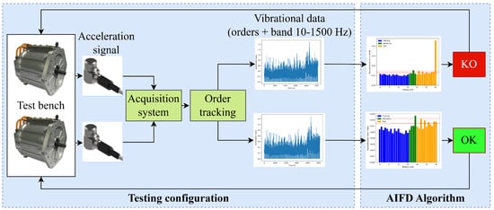
Figure 3.
Electric motor testing process with AIFD.
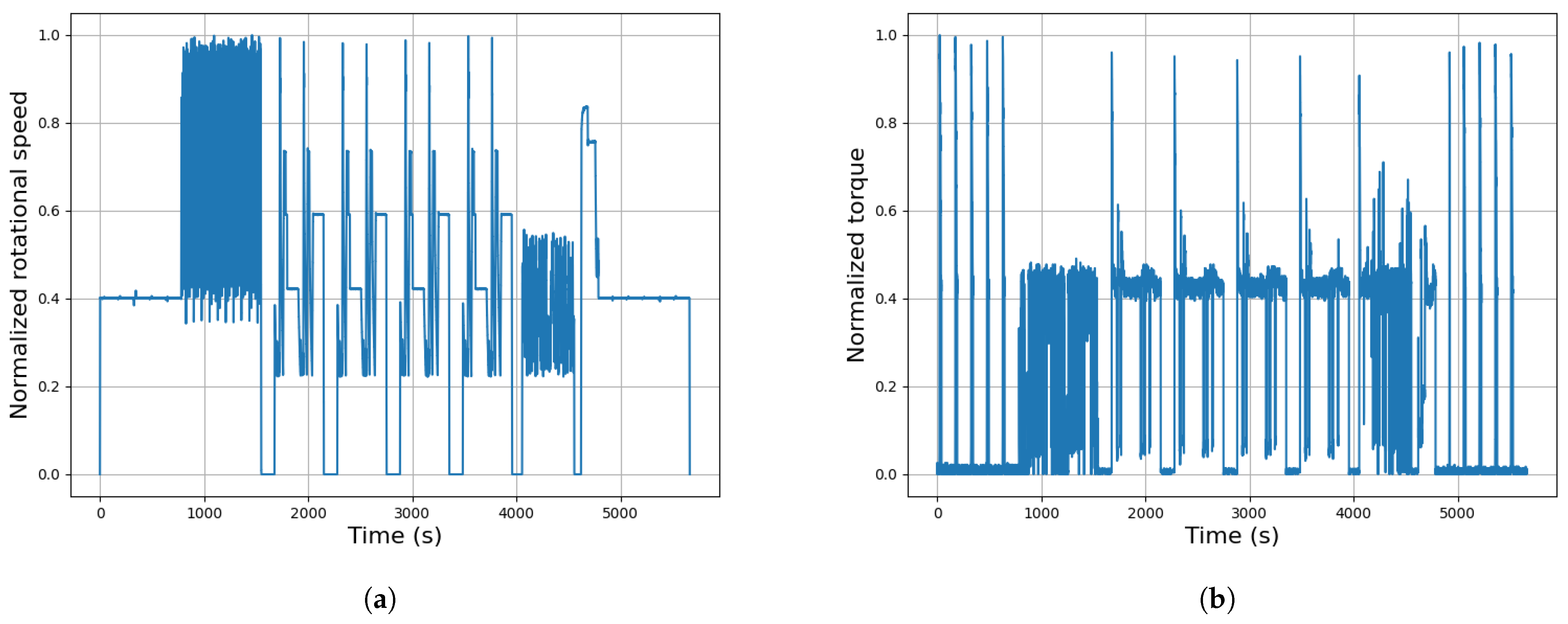
The test bench setup consists of two Permanent Magnet Synchronous Motors arranged in a back-to-back configuration. One motor provides the necessary torque as the traction motor, while the other absorbs the energy as a dynamic brake. Each motor is equipped with a mono-axial accelerometer to measure vibrations during the test, which lasts 1.5 h, which is followed by a same-length period where the motors remain stationary. This cycle is repeated for hundreds of tests to evaluate the lifespan of PMSMs under various combinations of low and high torque and speed (shown in Figure 4), with the added challenge of extreme environmental conditions like high and low temperatures and humidity. This makes fault detection critical, as harsh conditions can lead to premature anomalies in the motor operation.

Figure 4.
Generic testing cycle normalised speed and torque profiles. (a) Speed profile, (b) torque profile.
An Artificial Intelligence Fault Detection (AIFD) algorithm, exploiting AEs, is introduced to monitor the motor’s condition during testing. The AIFD algorithm analyses the extracted accelerometer data to determine whether the motor is in an “OK” or “KO” state. If the motor is in a “KO” state, the algorithm immediately stops the test.
3.2. Analysed Data
Three different typologies of PMSMs (namely Alpha, Beta and Gamma) have been analysed in order to evaluate the performances of the six AEs. Each typology includes different samples of the same electric motor, as detailed in Table 1, where the final status of each tested PMSM is shown. The accelerometer data is acquired at a sampling frequency of 50 kHz and processed by the order tracking technique [34] to extract key vibration orders such as mechanical, electromagnetic and bearing ones, providing a detailed analysis of the motor’s dynamic behaviour. The system records processed vibration data every 0.25 s (4 Hz).

Table 1.
Status of the electric motors used for the definition of the Autoencoder. Alpha, Beta and Gamma represent three different PMSM topologies being tested. NF: no fault detected. DE: drive end.
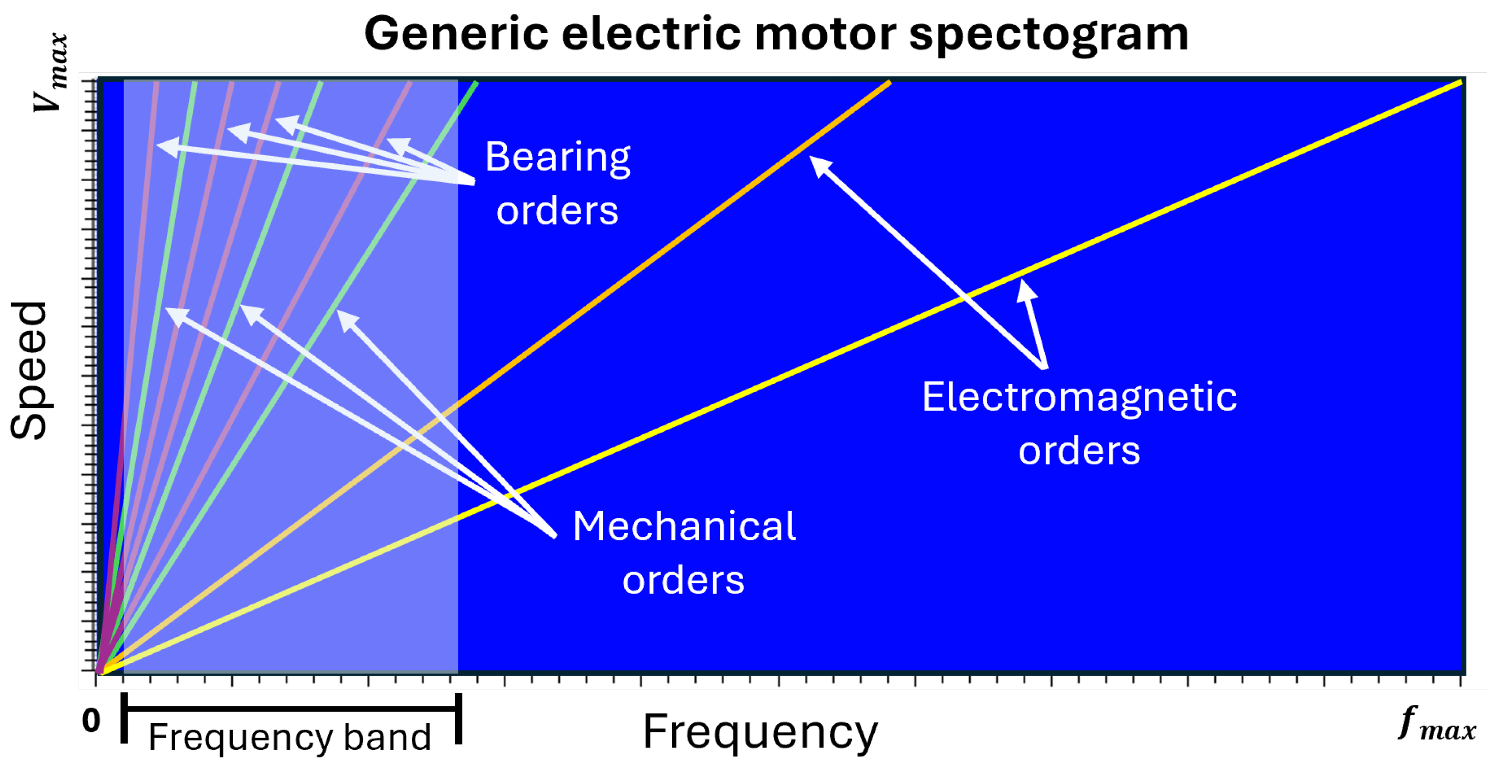
The input variables considered for the evaluation of the proposed AE architectures are shown in the spectrogram of Figure 5. They are the following:

Figure 5.
Generic PMSM spectrogram showing mechanical orders, bearing and electromagnetic orders as a function of speed and frequency. The considered frequency band ranges from 10 Hz to 1500 Hz, covering key spectral components related to faults.
- Mechanical orders: The first two orders (1.00 and 2.00) are retained as they have a higher energy level and can provide details regarding rotor failures [35].
- Bearing orders: Even though BPFO (Ball Passing Frequency on the outer race) and BPFI (Ball Passing Frequency on the inner race) have been demonstrated to be the preferred frequencies for fault detection [35], all the following bearing orders have been extracted, including FTF (Fundamental Train Frequency) and BSF (Ball Spin Frequency):where n is the number of rolling elements present in the bearing, is the rotational frequency of the rotor and is the contact angle. and represent, respectively, the ball diameter and the pitch diameter of the bearing [36].
- Electromagnetic orders: Due to their high energy content, their amplitude is only marginally modified by the presence of a failure. Therefore, they were excluded from the analysis in this study.
- Vibration amplitude at 10–1500 Hz: This range is selected as it may contain critical fault detection details that broader bands could miss due to interference from high-energy electromagnetic orders, which can obscure finer signals. This input is valuable to the network because, in the presence of failures, certain bearing vibration orders may exhibit a modulation effect [37]. To obtain a single representative value, the 10–1500 Hz frequency band is expressed as the sum of all its components at each sampling time.
This multi-variable dataset undergoes several preprocessing stages to create the correct input for the AEs. The first step is to isolate the test cycles and reduce their dimensions through time averaging. This process minimises the impact of “distracting” data, such as noise and outliers, and improves the computational efficiency of the NNs. The number of windows to apply is calculated using the following formula:
This formula guarantees a data reduction by at least a factor of 40 while ensuring that the resulting length is a power of 2. This condition may be useful during the AE hyperparameter setting [38]. Next, as the datasets have to be used to compare and identify the best AE architecture, the data is normalised and reshaped into smaller 2D blocks, with each block representing one test cycle. This reshaping makes it easier for the AE to learn and identify hidden data patterns during training. The initial dataset with dimensions (total length, number of features) is reshaped into (number of cycles, cycle length, number of features), as shown in Figure 6.
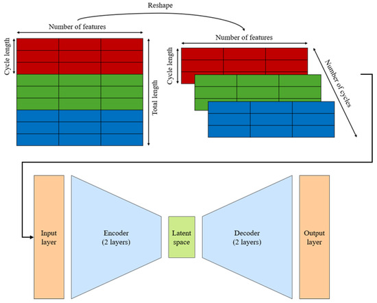
Figure 6.
Reshaping technique and input into the AE.
3.3. Autoencoders
The main architecture of the tested AEs is reported in Figure 1; other key design hyperparameters include the following:
- Activation function: ReLU.
- Normalisation: Min–Max, to scale acceleration data before input into the network.
- Batch size: 4, due to the limited number of training samples.
- Optimiser and loss function: The Adam optimiser is employed for its efficiency and fast convergence [25]. The MSE is computed for each variable and then averaged. For VAEs, the loss function additionally incorporates the KL divergence term, introduced in Section 2.
- Epochs and early stopping: Training proceeds for up to 250 epochs, with early stopping triggered if validation loss stagnates or increases within a tolerance of .
- Regularisation: An L2 regularisation term is incorporated into the loss function to encourage meaningful feature representations.
- Dropout: Applied only to neuron-based AEs to mitigate overfitting in fully connected layers.
Training data selection assumes that the electric motor starts in a healthy state, with the first testing cycles representing normal operation, free from wear-related faults. This assumption allows the model to train on healthy data, improving the reliability of defect detection in later cycles. A sensitivity analysis determined that 20 cycles provide the best balance between speed and accuracy, with an 80%–20% split into train and validation sets.
3.4. Grid Search Operation
To optimise the AE architectures, a multi-step grid search was implemented to refine parameter selection. The process started with the 1D CNN AE, as it has fewer trainable weights and shorter training times, allowing for a faster search. The ranges of parameters explored during the grid search are shown in Table 2.
Table 2.
Ranges of the parameters varied during the grid search (1D CNN AE).
The grid search followed these steps:
- Select model parameters and their initial values.
- Generate all possible parameter combinations.
- Train and evaluate validation errors.
- Select the top 5 networks (with respect to the validation error) and refine their parameters through an infill process, creating new variables in between the ones used in the previous step, and adjusting them based on the best-performing configurations.
- Repeat until validation error stabilises.
A total of 6 grid search infill steps were required to obtain stable results for the 1D CNN AE. For other AE types, extensive grid search was avoided due to the expensive computational effort. Instead, their architectures were initialised based on similarity to the 1D CNN AE and parameters were adjusted one at a time (OAT) to match validation performance (validation error and reconstruction quality) while considering computational efficiency. Then, fine-tuning was performed OAT to further reduce error rates, achieving a validation error in the range.
The final optimised parameters for all architectures are reported in Table 3, grouping networks by shared base units while differing in latent space configurations.
Table 3.
Optimised parameters of each proposed architecture.
4. Results and Discussion
In order to compare the six AE architectures, different metrics have been taken into account: training behaviour, reconstruction accuracy, reconstruction error history, model accuracy and network speed.
4.1. Training Process
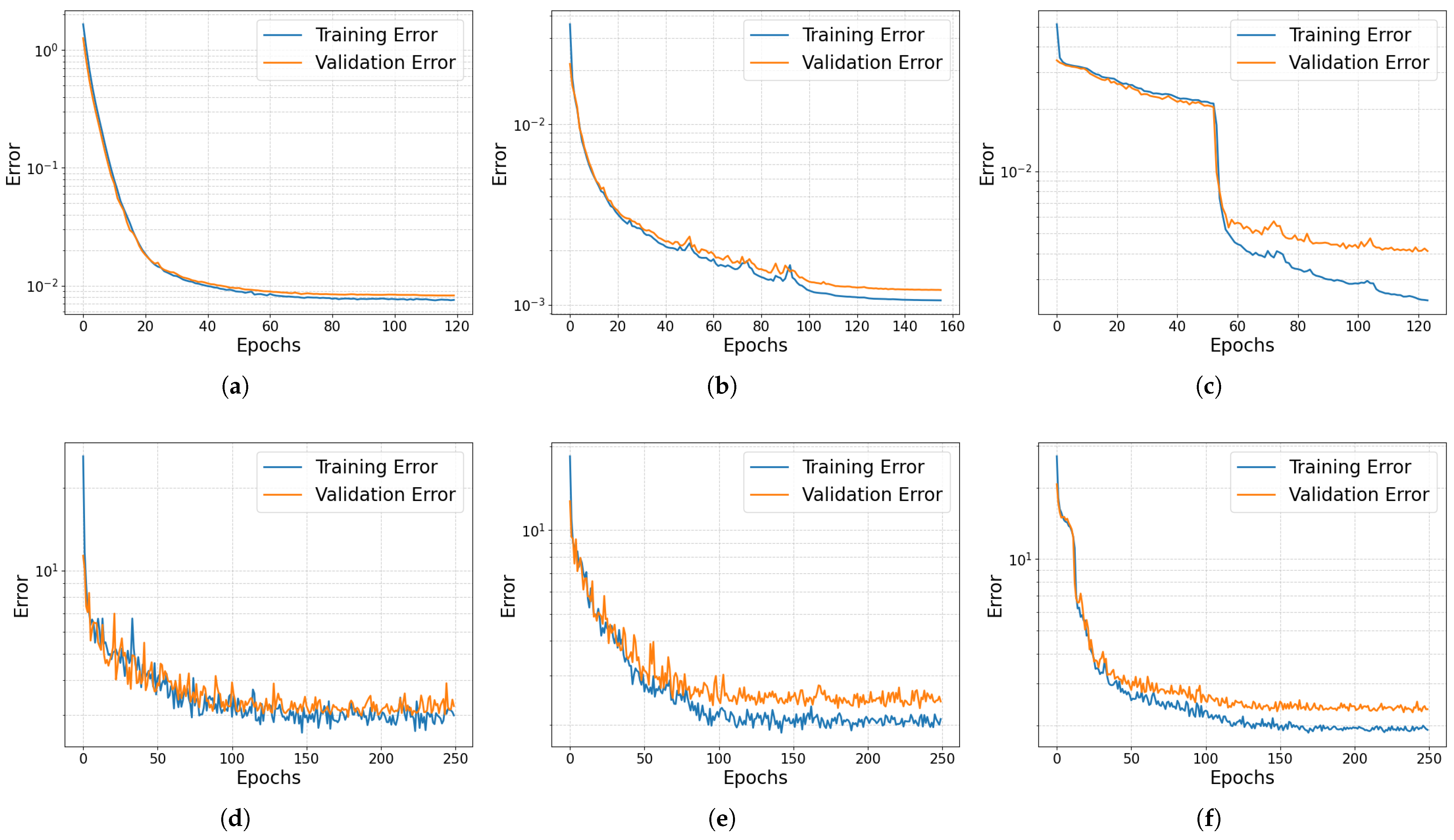
The initial evaluation assesses training performance by examining the stability of training and validation errors, which are illustrated in Figure 7. CNN AEs (Figure 7b,e) outperform both neuron-based AEs (Figure 7a,d) and LSTM AEs (Figure 7c,f) by achieving a lower training error, ensuring better reconstruction accuracy, while maintaining a good stability. Compared to the 1D CNN VAE (Figure 7e), the 1D CNN AE (Figure 7b) shows higher training stability, steady errors and faster convergence, implying better generalisation [39]. The direct comparison between the training and validation error of VAEs and AEs is not possible due to the presence of the KL-loss term in the VAE loss function, as stated in Equation (4).
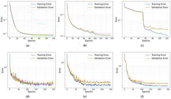
Figure 7.
Training and validation errors (Alpha 1001). (a) AE, (b) 1D CNN AE, (c) LSTM AE, (d) VAE, (e) 1D CNN VAE, (f) LSTM VAE.
Table 4 summarises the training performance achieved by each architecture during the training process for the analysis of a specific motor. Networks with fewer weights (1D CNN AE and LSTM AE) require less data for training. However, the LSTM AE’s lower weight count is due to constraints on training time and resources. Therefore, the LSTM AE struggles with stable training, as shown in Figure 7c, suggesting lower accuracy. Increasing the number of LSTM units could improve accuracy but would also significantly increase computational costs.
Table 4.
Training performance of each architecture for a specific PMSM. denotes the number of evaluated weights during the training process, is the final training error, is the final validation error, represents the standard deviation over the last 50 training epochs and represents the standard deviation over the last 50 validation epochs.
4.2. Value
The value [40] is used to assess the reconstruction capabilities of the analysed AEs, indicating the discrepancy between the original and the reconstructed data. It is calculated only on the training set, as including faulty data would invalidate the calculation. A value close to 1 indicates high reconstruction accuracy. The results, as shown in Table 5, indicate that the 1D CNN AE achieves the highest reconstruction accuracy, with an average value closer to 1. In contrast, standard AE and VAE models perform poorly, failing to accurately capture the input signal. The LSTM AE shows some improvements but with inconsistent precision, heavily influenced by the considered dataset.
Table 5.
comparison.
4.3. Reconstruction Comparison
To assess the accuracy of each AE architecture, the reconstruction error is analysed. The reconstruction error evaluates the difference between the input orders () and those reconstructed by the AEs (). This metric helps to distinguish between faulty and non-faulty motors, as AEs struggle to accurately reconstruct anomalous data: higher errors indicate potential faults, while normal data yields lower errors. To quantify the reconstruction error, the Mean Absolute Error (MAE) is used. The choice of MAE, for example over MSE, was motivated by the excessive variability observed in reconstruction errors on the test set when using MSE. MAE provides a more stable and robust evaluation metric, being less sensitive to outliers and more consistent for defining fault detection thresholds [21]. The MAE is calculated on each dataset variable and then averaged to obtain a single value, as shown in the following equations:
where m represents the number of features and n denotes the number of data points.
To classify each testing cycle, a threshold is required to separate normal and faulty conditions. The threshold must be defined based on the training and validation datasets, as they contain only healthy data. This ensures a reliable reference for normal operating conditions, allowing any value exceeding the threshold to be classified as faulty. In this work, two thresholds are adopted, as proposed by Givnan et al. [17]: the lower threshold aims to detect the onset of a potential anomaly (warning), while the higher threshold is used to flag more severe faults. Both thresholds are computed statistically by considering the interquartile range (IQR) as a measure of data dispersion, following the approach of Lee et al. [8]. In our case, the higher threshold is defined as two times the IQR above the warning level:
where Q3, the third quartile, represents the value below which 75% of the training and validation data fall, while the IQR is calculated as follows:
where Q1, the first quartile is the value below which only 25% of the training and validation data fall.
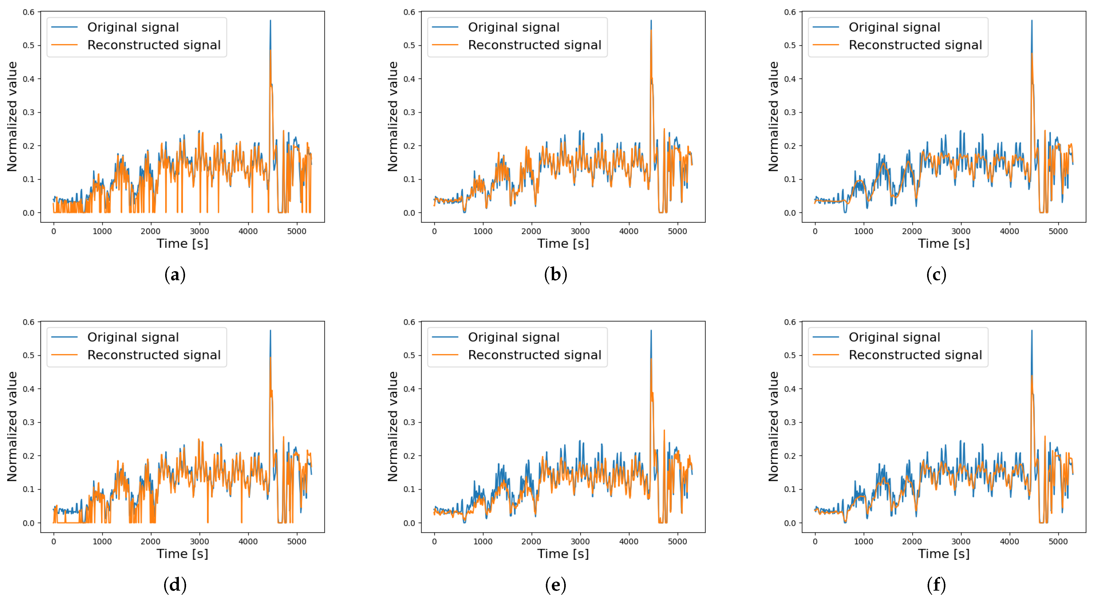
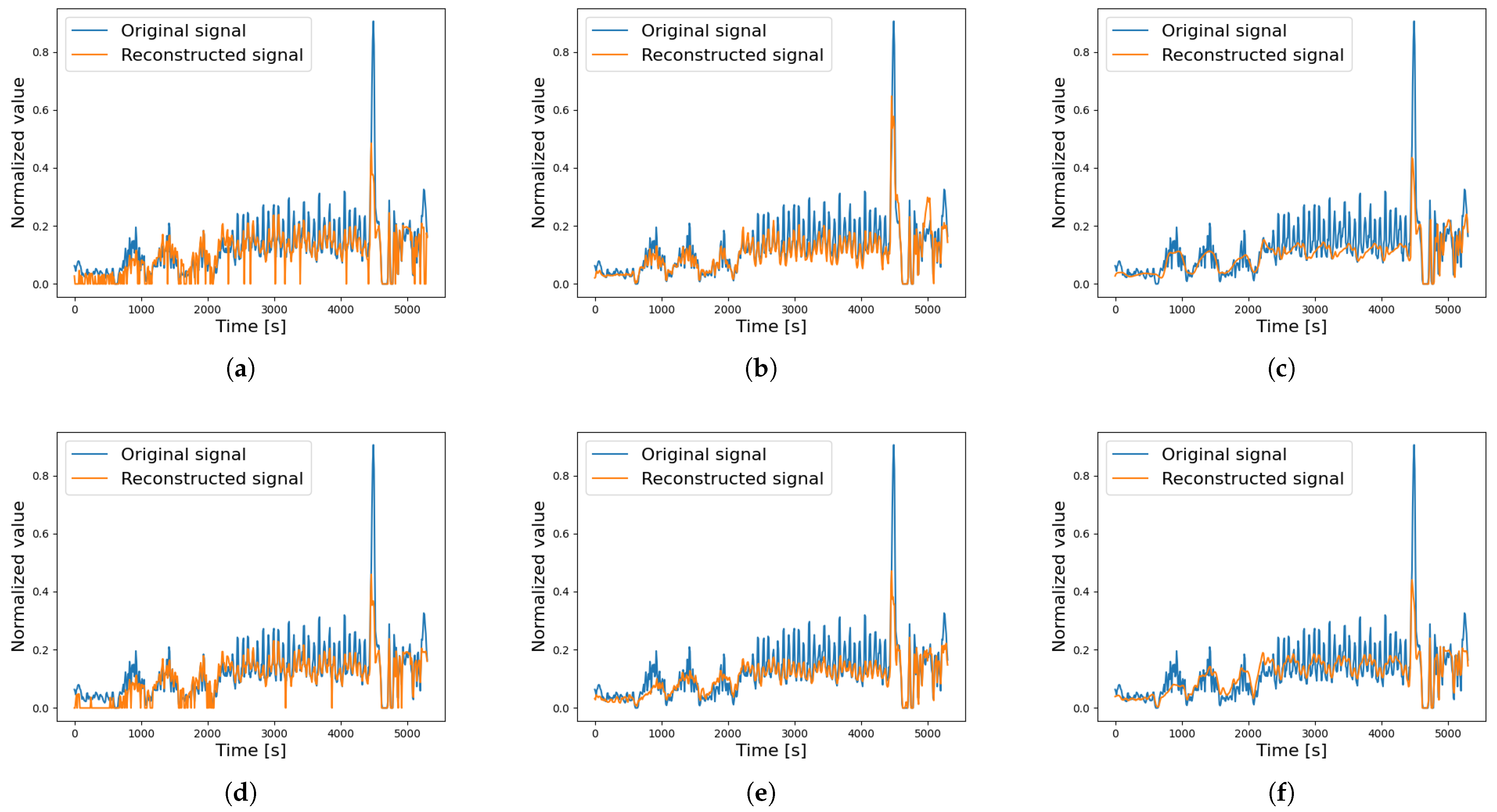
A comparison of the reconstructed signals is presented to better understand the behaviour of the different AEs under both non-faulty and faulty motor conditions. Specifically, the analysis focuses on motor Beta 1001, which was later found to have a broken DE bearing. The motor started to show signs of wear during the 80th cycle, as the average acceleration value calculated for order 6.95 (associated with the broken DE bearing) increased by 87% after this cycle. Figure 8 compares the reconstructed signal (BPFI ORD 6.95) across the different AEs during a non-faulty cycle. The standard AE and VAE exhibit low accuracy, often producing null values for low-amplitude signals. The LSTM AEs approximate the signal as an average, reducing noise but also smoothing out critical peaks. The 1D CNN AE demonstrates the best reconstruction accuracy, better capturing the full time history of the original signal. Instead, Figure 9 shows the reconstruction signals for a faulty cycle, where each AE struggles to accurately reconstruct the original signal, highlighting the presence of a fault. As seen in Figure 8 and Figure 9, the input signals differ significantly, but since the Autoencoders are trained on identical training cycles, faults are clearly evident in the second case.
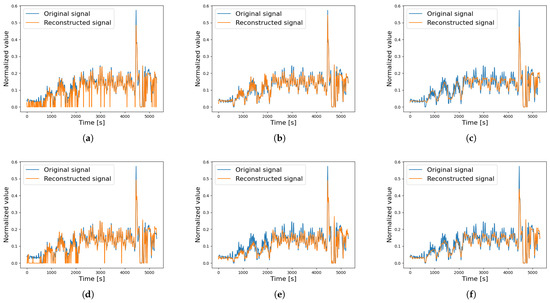
Figure 8.
Reconstructed signal of a single testing cycle—non-faulty data, BPFI ORD 6.95 (Beta 1001). (a) AE, (b) 1D CNN AE, (c) LSTM AE, (d) VAE, (e) 1D CNN VAE, (f) LSTM VAE.
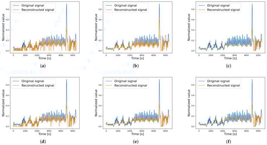
Figure 9.
Reconstructed signal of a single testing cycle—faulty data, BPFI ORF 6.95 (Beta 1001). (a) AE, (b) 1D CNN AE, (c) LSTM AE, (d) VAE, (e) 1D CNN VAE, (f) LSTM VAE.
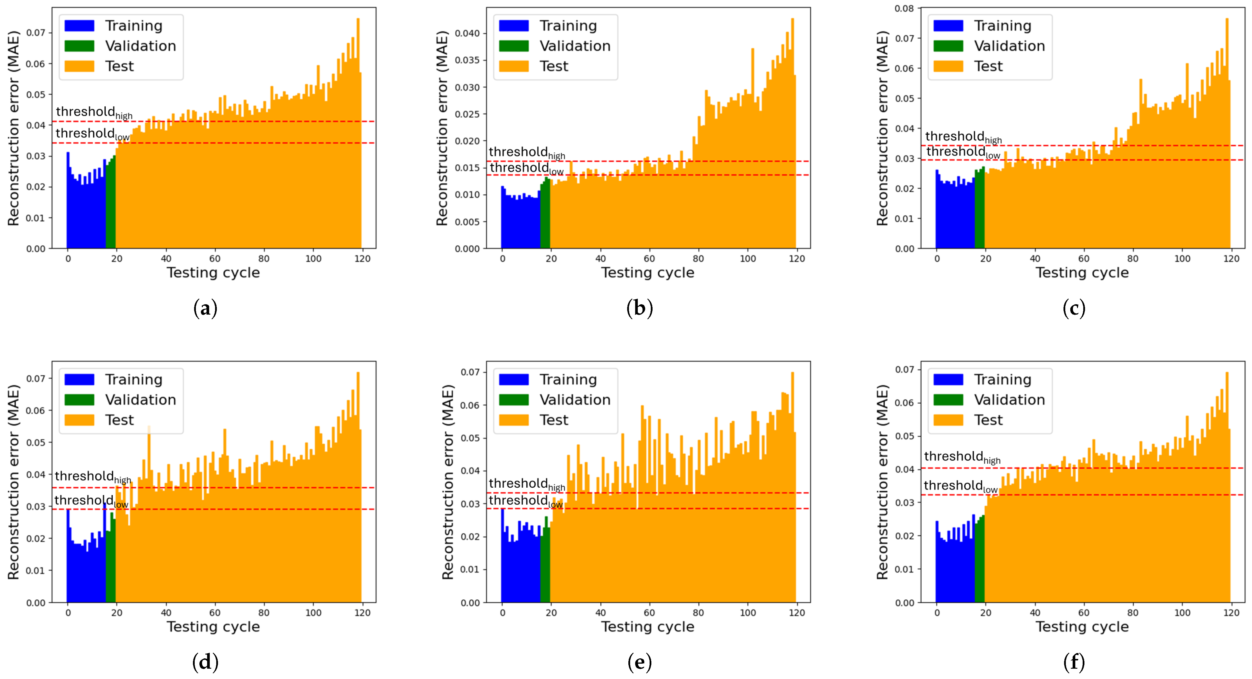
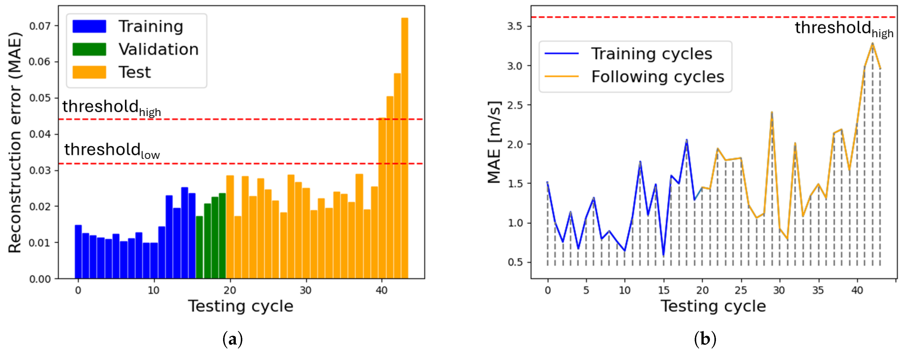
Finally, Figure 10 illustrates the reconstruction error trends over the entire duration cycle for the motor across the six different networks. While all AEs ultimately classify the motor as faulty, their behaviours vary. The 1D CNN AE performs best, with a steady error increase until the 80th cycle, where a sharp increase suggests an internal change. The AE, VAE and 1D CNN VAE show high variability, causing false alarms before the 80th cycle. The LSTM VAE struggles with generalisation, showing an early error spike. The LSTM AE also performs well but lacks the distinct error shift of the 1D CNN AE, making its fault detection less reliable. In addition, Figure 10b shows that once the higher threshold is exceeded, the MAE progressively increases. This behaviour can be interpreted as the result of cumulative component wear.
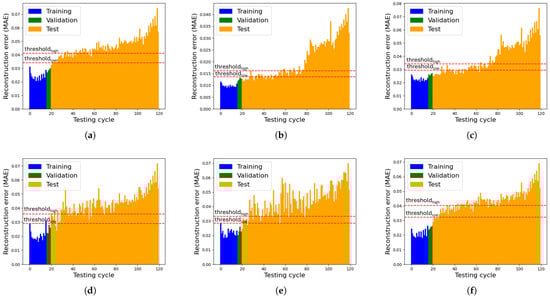
Figure 10.
Reconstruction errors (Beta 1001, 2nd dataset). (a) AE, (b) 1D CNN AE, (c) LSTM AE, (d) VAE, (e) 1D CNN VAE, (f) LSTM VAE.
4.4. Model Accuracy
Different classification metrics have been evaluated to assess model performance: accuracy, precision, recall and F1-score [21]. The metric accuracy indicates the proportion of correct predictions over the total dataset. Precision refers to the percentage of positive predictions that are actually correct, while recall measures the ability of the model to identify all true positive instances. The F1-score, calculated as the harmonic mean of precision and recall, balances the two metrics [21]. It is especially useful in imbalanced datasets, where high accuracy alone may be misleading. In general, performance closer to 100% is considered more desirable. All these metrics are derived from four fundamental quantities: true positive (TP), false positive (FP), true negative (TN) and false negative (FN). These values were computed by comparing the reconstruction error of each testing cycle with respect to the highest threshold. For cycles preceding the failure point, FP was assigned when the threshold was exceeded and TN when it was not. For cycles following the failure point, TP was assigned when the threshold was exceeded, and FN when it was not. Each classification metric was computed individually for each motor listed in Table 1. The final values reported in Table 6 represent the average over all motors and were evaluated for the six proposed network architectures, providing a comprehensive indication of the overall model performance.
Table 6.
Model accuracy comparison.
The 1D CNN AE model delivers the best overall performance, with the highest accuracy, perfect recall and the best F1-score, indicating excellent reliability and balance between detection and precision. Compared to other models, it not only captures all true positives but also maintains a high precision, minimising false alarms. In contrast, the standard VAE exhibits the lowest F1-score, reflecting weaker performance in distinguishing faults. While incorporating CNN and LSTM layers into the VAE leads to slight improvements, these variants still underperform compared to the AE-based counterparts.
4.5. Network Speed
This comparison focuses on training and evaluation speeds, particularly important for real-time implementation. The tests were conducted on a system with an Intel Core i5-12500H CPU (12 cores, 16 threads, 2.5 GHz) and 16 GB DDR4 RAM, running Windows 11.
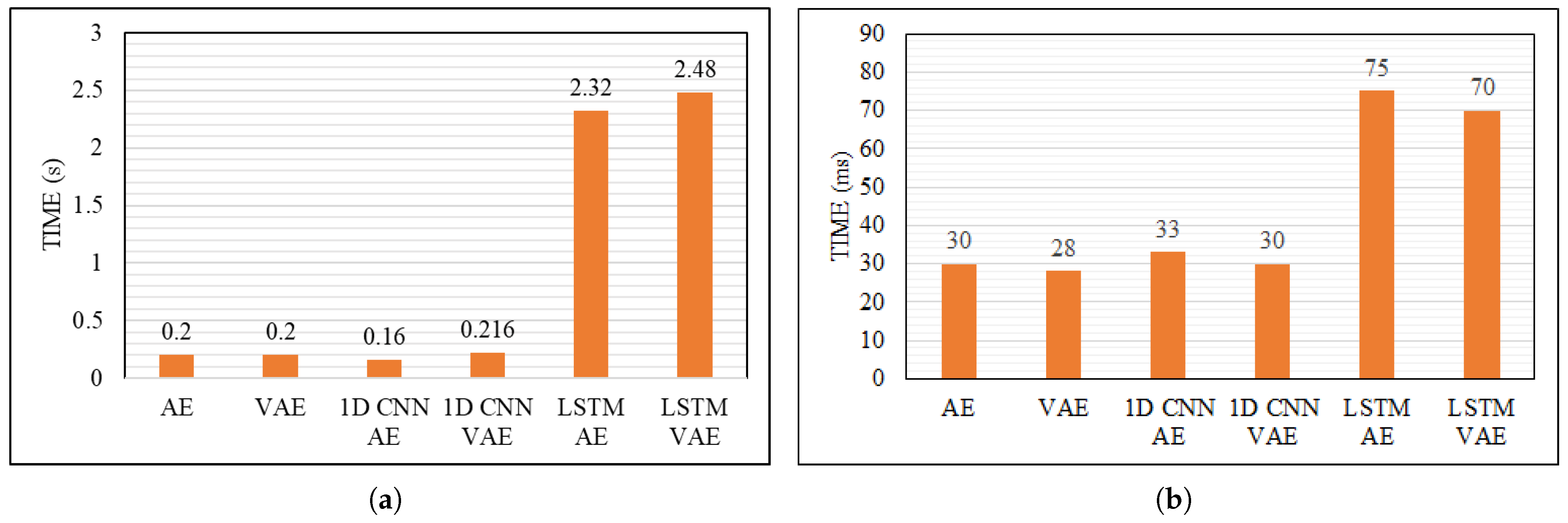
Considering the duration of the training (Figure 11a), the 1D CNN AE is the fastest, requiring an average of 160 ms per epoch, whereas LSTM-based AEs take over 2 s. This higher training time, combined with the need for more data to improve accuracy, makes LSTM-based models less efficient for real-time applications. Regarding the evaluation step (Figure 11b), LSTM AEs remain the slowest, while the other models exhibit similar yet superior performance.
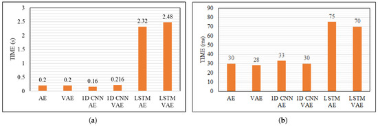
Figure 11.
Training and evaluation times. (a) Training time per epoch, (b) evaluation time per epoch.
4.6. Final AEs Comparison
Table 7 compares the performance of all the tested networks. The 1D CNN AE results to be the best choice for unsupervised fault detection in PMSMs, offering superior accuracy and efficiency. Its ability to work with limited information makes it particularly suitable for scenarios with restricted data availability. Overall, the 1D CNN AE provides the best balance of accuracy, efficiency and practicality.
Table 7.
Network performance comparison on PMSM fault detection. + stands for positive behaviour, while - stands for negative behaviour in the respective feature. Multiple signs (e.g., +++, - -) indicate increasing intensity of the corresponding behaviour.
4.7. Comparison with Traditional Metrics
This section introduces two traditional techniques for analysing accelerometer signals to detect early fault indications. These methods are then compared to the 1D CNN AE, as it has been demonstrated to be the best-performing NN, in order to display the advantages of the AI-based approach over common metrics.
The first method is the mean acceleration signal analysis [41] which considers the same signals used for AE training (mechanical orders, bearing orders and the vibration amplitude at 10–1500 Hz), applying the same normalisation process to ensure a fair comparison. The average value of each variable over a testing cycle is computed as
where n is the number of time points and m the extracted features. Then, the mean across all variables is calculated as
In Figure 12, the comparison between the 1D CNN AE and the mean acceleration value is presented for motor Beta 1001. The AE shows a clear problem after 80 testing cycles, as the MAE drastically increases. On the other hand, the mean acceleration value shows an unusual pattern: it first decreases at the beginning and then starts to rise until the final cycle, but the error never reaches a critical value to indicate a potential and certain fault. The 1D CNN AE effectively detected anomalies at an earlier stage, demonstrating the robustness of the proposed approach in identifying impending failures before they become noticeable through conventional methods.
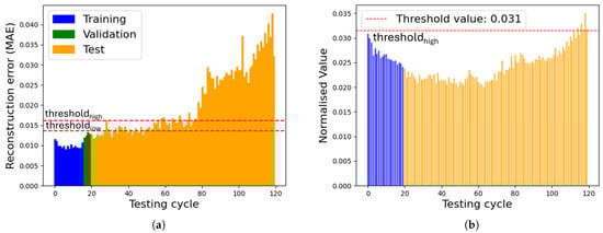
Figure 12.
AE vs. mean acceleration value (Beta 1001). (a) Reconstruction error 1D CNN AE, (b) mean acceleration value.
The second metric calculates the MAE of the vibration amplitude at 10–1500 Hz [42], a key indicator of motor condition. First, the average value over the first 20 cycles used in the training process is computed for each time point:
Then, the point-by-point discrepancy of each testing cycle relative to this average is calculated as
where K is the total number of testing cycles. This metric is also applied to training cycles to better compare results.
Figure 13 compares the 1D CNN AE output with the MAE of the frequency band for motor Alpha 1005. The 1D CNN AE output clearly indicates a problem, as the reconstruction error exceeds the set thresholds starting from cycle 40. After three additional cycles, the motor has been stopped due to the test bench vibration alarm and confirmed to be faulty due to a seized drive end bearing. In contrast, the 10–1500 Hz vibration amplitude does not show a consistent trend. This, combined with the fact that the MAE calculated on this frequency band never reaches the pre-established threshold, highlights the effectiveness of the 1D CNN AE as a more robust fault indicator.
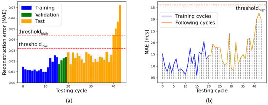
Figure 13.
AE vs. MAE frequency band (Alpha 1005). (a) Reconstruction error 1D CNN AE, (b) MAE 10–1500 Hz.
The findings of the faulty test cases presented in Table 1 are summarised in Table 8, which highlights the importance of a more detailed approach to monitor motor health. In fact, the 1D CNN AE is better at spotting small changes than traditional methods, like the average acceleration or the MAE of a frequency band. To further validate the 1D CNN AE’s robustness, we also processed the motors listed as non-faulty in Table 1. The AE correctly identified these motors as non-faulty, demonstrating its reliability even in the absence of issues.
Table 8.
Detection capabilities: 1D CNN AE vs. traditional metrics.
4.8. AIFD Algorithm
In the proposed monitoring framework, each operating cycle refers to a complete test run of the PMSM under defined conditions. The 1D-CNN Autoencoder has been integrated into a complete algorithm for direct online monitoring of PMSM testing, effectively identifying potential faults as well as anomalies in the measurement system. Since the motor is expected to perform hundreds of such cycles over the course of the durability test, the duration of a single cycle is relatively short compared to the total test time. Hence, the AIFD algorithm operates in a “semi-real-time” manner, as each cycle is evaluated only after its completion, requiring access to the full dataset for proper assessment. The algorithm has been developed using Python 3.11.7, TensorFlow 2.17.0 and Anaconda Suite 24.4.0.
The designed software enables the parallel analysis of multiple motors running the durability test. Test data related to each motor are updated in real time and saved on a dedicated repository, where they are processed for training and for the continuous monitoring of newly available testing cycles. The algorithm allows users to configure network parameters, adjust fault detection thresholds and retrain the model with custom datasets, ensuring optimal performance under varying conditions. A dedicated interface, shown in Figure 14 provides real-time alerts, displays processing status and visualises reconstruction error plots for fault analysis.
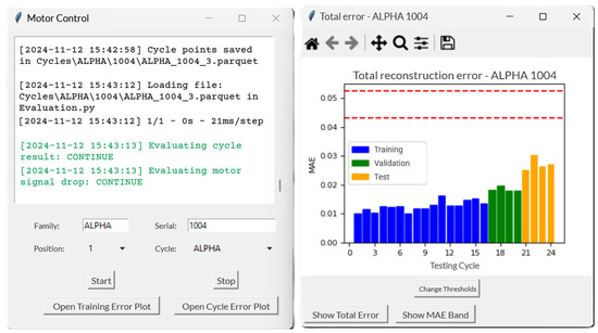
Figure 14.
The fault detection algorithm at work.
Following its installation on the electric motor test bench on 28 October 2024, the AIFD algorithm has evaluated approximately 5000 testing cycles across twenty motors. With the new monitoring system, compared to the previous approach which relied on a fixed acceleration threshold for each order, the downtime of the test bench has been halved. The algorithm successfully identifies failures in PMSMs, revealing issues that were difficult to be detected using the previous standard monitoring method. These results highlight the system’s effectiveness in enhancing fault detection for PMSMs.
5. Conclusions
This research presents an Artificial Intelligence-based strategy for effective fault detection of electric motors for the automotive sector, specifically during the endurance testing of PMSMs. A comprehensive literature review identified Autoencoders as a promising Machine Learning techniques for fault detection. However, unlike most existing studies, which focus on steady-state conditions at constant speed, this approach addresses a gap in the literature by analysing motors under challenging conditions with continuous variations in speed and torque. Moreover, another important innovation is the use of the least amount of training data (only 20 testing cycles) to accelerate network creation, minimising time loss in the industrial context while maintaining a good level of accuracy. The method exploits vibrational data from the order domain, including mechanical and bearing orders, as well as the vibration amplitude in the band 10–1500 Hz.
Six different Autoencoder architectures were compared to determine the most effective one on this specific application: the standard AE, the VAE, the 1D CNN AE, the 1D CNN VAE, the LSTM AE and the LSTM VAE. These networks were trained on vibrational data and assessed based on their reconstruction error. Among them, the 1D CNN AE emerged as the top performer, achieving superior accuracy (91% and 95.3% F1-score), faster processing (on average 32% faster than the other networks), lower computational effort (57% less weights to be initialised) and reduced data requirements (utilising only 20 cycles for training while maintaining a good accuracy). The proposed algorithm is able to detect various mechanical faults and control-related anomalies. The method was validated on five motors, successfully identifying bearing faults, shaft misalignments and wear processes that conventional monitoring techniques were unable to capture. In fact, a comparison with traditional fault detection metrics (mean acceleration value and MAE of the vibration amplitude at 10–1500 Hz) revealed that the 1D CNN AE overcomes their major limitations. While traditional metrics often struggle with fault detection and lack robustness, the 1D CNN AE demonstrated exceptional predictive capabilities, issuing early warnings up to 40 test cycles in advance. This can enable proactive maintenance, minimising costly repairs and optimising system reliability.
The 1D CNN AE was integrated into a Python-based fault detection algorithm (AIFD) for semi-real-time monitoring of PMSM testing at the test bench. The AIFD system can stop the test by raising alarms and offers user-configurable settings for optimal training and monitoring. Additionally, the AIFD system has significantly reduced downtime (up to 50%) on the test bench compared to the previous monitoring system.
This research demonstrates the effectiveness of AI-driven fault detection in challenging testing environments characterised by highly variable speed and torque conditions. The findings highlight the potential for future advancements that could further enhance reliability and operational efficiency in the automotive sector.
Several proposals for future research emerge from the topics covered in this study:
- Reducing the need for multiple models: A new network is required for each motor tested, which may be redundant. Future work should focus on developing an AE that generalises across motors with similar architectures.
- Expanding the dataset: Incorporating additional signals, such as current and temperature, could improve fault detection accuracy.
- Integrating fault classification: Adding a classifier to the 1D CNN AE could help identify specific faults, but this would require a large and labelled dataset.
Author Contributions
Conceptualisation, F.S., D.B. and M.G.; methodology, I.C., F.S. and D.B.; software, I.C.; validation, I.C., F.S. and D.B.; formal analysis, F.S., D.B. and M.G.; investigation, I.C.; resources, M.G. and G.M.; data curation, I.C., F.S. and D.B.; writing—original draft preparation, I.C., F.S. and D.B.; writing—review and editing, M.G., F.M.B. and G.M.; visualisation, I.C., F.S. and D.B.; supervision, M.G., F.M.B. and G.M.; project administration, M.G. All authors have read and agreed to the published version of the manuscript.
Funding
This research received received partial funding from the European Union Next-Generation EU (PIANO NAZIONALE DI RIPRESA E RESILIENZA (PNRR)—MISSIONE 4 COMPONENTE 2, INVESTIMENTO 1.4—D.D. 1033 17 June 2022, CN00000023).
Data Availability Statement
The original contributions presented in the study are included in the article; further inquiries can be directed to the corresponding author.
Conflicts of Interest
The authors declare no conflicts of interest.
Abbreviations
The following abbreviations are used in this manuscript:
| AE | Autoencoder | MAE | Mean Absolute Error |
| AI | Artificial Intelligence | ML | Machine Learning |
| AIFD | Artificial Intelligence Fault Detection | MLP | Multilayer Perceptron |
| ANN | Artificial Neural Network | MSE | Mean Square Error |
| BPFI | Ball Passing Frequency on the inner race | NN | Neural Network |
| BPFO | Ball Passing Frequency on the outer race | OAT | One parameter at a time |
| BPTT | Backpropagation Through Time | OC-SVM | One-Class Support Vector Machine |
| BSF | Ball Spin Frequency | PCA | Principal Component Analysis |
| CNN | Convolutional Neural Network | PdM | Predictive maintenance |
| DC | Direct current | PHM | Prognostics and health management |
| DL | Deep Learning | PMSM | Permanent Magnet Synchronous Motor |
| ELBO | Evidence Lower Bound | ReLU | Rectified Linear Unit |
| FFT | Fast Fourier Transform | RNN | Recurrent Neural Network |
| FTF | Fundamental Train Frequency | RSAE | Reduced Stacked Autoencoder |
| GRU | Gated Recurrent Unit | SSR | Sum of Squared Residuals |
| IoT | Internet of Things | SST | Total Sum of Squares |
| IQR | Interquartile range | SW-DAE | Sliding Window Denoising Autoencoder |
| KL | Kullback–Leibler | TTD | Time to Detect |
| LSTM | Long Short-Term Memory | VAE | Variational Autoencoder |
References
- Zonta, T.; da Costa, C.A.; da Rosa Righi, R.; de Lima, M.J.; da Trindade, E.S.; Li, G.P. Predictive maintenance in the Industry 4.0: A systematic literature review. Comput. Ind. Eng. 2020, 150, 106889. [Google Scholar] [CrossRef]
- Huang, C.; Bu, S.; Lee, H.H.; Chan, K.W.; Yung, W.K. Prognostics and health management for induction machines: A comprehensive review. J. Intell. Manuf. 2024, 35, 937–962. [Google Scholar] [CrossRef]
- Mohammadi, M.; Al-Fuqaha, A.; Sorour, S.; Guizani, M. Deep Learning for IoT Big Data and Streaming Analytics: A Survey. IEEE Commun. Surv. Tutorials 2018, 20, 2923–2960. [Google Scholar] [CrossRef]
- Qiu, S.; Cui, X.; Ping, Z.; Shan, N.; Li, Z.; Bao, X.; Xu, X. Deep Learning Techniques in Intelligent Fault Diagnosis and Prognosis for Industrial Systems: A Review. Sensors 2023, 23, 1305. [Google Scholar] [CrossRef]
- Bono, F.M. Deep Learning for Fault Detection in Complex Mechanical Systems. Master’s Thesis, Politecnico di Milano, Milano, Italy, 2023. Available online: https://hdl.handle.net/10589/213472 (accessed on 27 September 2024).
- Yang, Z.; Xu, B.; Luo, W.; Chen, F. Autoencoder-based representation learning and its application in intelligent fault diagnosis: A review. Meas. J. Int. Meas. Confed. 2022, 189, 110460. [Google Scholar] [CrossRef]
- Chen, S.; Yu, J.; Wang, S. One-Dimensional Convolutional Auto-Encoder-Based Feature Learning for Fault Diagnosis of Multivariate Processes. J. Process Control 2020, 87, 54–67. [Google Scholar] [CrossRef]
- Lee, G.; Jung, M.; Song, M.; Choo, J. Unsupervised Anomaly Detection of the Gas Turbine Operation via Convolutional Auto-Encoder. In Proceedings of the 2020 IEEE International Conference on Prognostics and Health Management (ICPHM), Detroit, MI, USA, 8–10 June 2020; pp. 1–6. [Google Scholar] [CrossRef]
- Ahmad, S.; Styp-Rekowski, K.; Nedelkoski, S.; Kao, O. Autoencoder-Based Condition Monitoring and Anomaly Detection Method for Rotating Machines. In Proceedings of the 2020 IEEE International Conference on Big Data, Atlanta, GA, USA, 10–13 December 2020; Institute of Electrical and Electronics Engineers Inc.: Piscataway, NJ, USA, 2020; pp. 4093–4102. [Google Scholar] [CrossRef]
- Wu, D.; Chen, D.; Yu, G. New Health Indicator Construction and Fault Detection Network for Rolling Bearings via Convolutional Auto-Encoder and Contrast Learning. Machines 2024, 12, 362. [Google Scholar] [CrossRef]
- Eren, L. Bearing Fault Detection by One-Dimensional Convolutional Neural Networks. Math. Probl. Eng. 2017, 2017, 8617315. [Google Scholar] [CrossRef]
- Li, H.; Zhu, Z.Q.; Azar, Z.; Clark, R.; Wu, Z. Fault Detection of Permanent Magnet Synchronous Machines: An Overview. Energies 2025, 18, 534. [Google Scholar] [CrossRef]
- Abood, S.; Annamalai, A.; Chouikha, M.; Nejress, T. Fault Diagnostics of Synchronous Motor Based on Artificial Intelligence. Machines 2025, 13, 73. [Google Scholar] [CrossRef]
- Bae, I.; Lee, S. A Multi-Input Convolutional Neural Network Model for Electric Motor Mechanical Fault Classification Using Multiple Image Transformation and Merging Methods. Machines 2024, 12, 105. [Google Scholar] [CrossRef]
- Principi, E.; Rossetti, D.; Squartini, S.; Piazza, F. Unsupervised Electric Motor Fault Detection by Using Deep Autoencoders. IEEE/CAA J. Autom. Sin. 2019, 6, 441–451. [Google Scholar] [CrossRef]
- Huang, Y.; Chen, C.H.; Huang, C.J. Motor Fault Detection and Feature Extraction Using RNN-Based Variational Autoencoder. IEEE Access 2019, 7, 139086–139096. [Google Scholar] [CrossRef]
- Givnan, S.; Chalmers, C.; Fergus, P.; Ortega-Martorell, S.; Whalley, T. Anomaly Detection Using Autoencoder Reconstruction upon Industrial Motors. Sensors 2022, 22, 3166. [Google Scholar] [CrossRef] [PubMed]
- Ince, T.; Kiranyaz, S.; Eren, L.; Askar, M.; Gabbouj, M. Real-Time Motor Fault Detection by 1-D Convolutional Neural Networks. IEEE Trans. Ind. Electron. 2016, 63, 7067–7075. [Google Scholar] [CrossRef]
- Afrasiabi, S.; Afrasiabi, M.; Parang, B.; Mohammadi, M. Real-Time Bearing Fault Diagnosis of Induction Motors with Accelerated Deep Learning Approach. In Proceedings of the 2019 10th International Power Electronics, Drive Systems and Technologies Conference (PEDSTC), Shiraz, Iran, 12–14 February 2019; pp. 155–159. [Google Scholar] [CrossRef]
- An, K.; Lu, J.; Zhu, Q.; Wang, X.; De Silva, C.W.; Xia, M.; Lu, S. Edge solution for real-time motor fault diagnosis based on efficient convolutional neural network. IEEE Trans. Instrum. Meas. 2023, 72, 3516912. [Google Scholar] [CrossRef]
- Choi, Y.; Joe, I. Motor Fault Diagnosis and Detection with Convolutional Autoencoder (CAE) Based on Analysis of Electrical Energy Data. Electronics 2024, 13, 3946. [Google Scholar] [CrossRef]
- Toma, R.N.; Piltan, F.; Kim, J.M. A deep autoencoder-based convolution neural network framework for bearing fault classification in induction motors. Sensors 2021, 21, 8453. [Google Scholar] [CrossRef]
- Kamat, P.; Marni, P.; Cardoz, L.; Irani, A.; Gajula, A.; Saha, A.; Kumar, S.; Sugandhi, R. Bearing fault detection using comparative analysis of random forest, ANN, and autoencoder methods. In Communication and Intelligent Systems: Proceedings of ICCIS 2020; Springer: Berlin/Heidelberg, Germany, 2021; pp. 157–171. [Google Scholar]
- Qian, J.; Song, Z.; Yao, Y.; Zhu, Z.; Zhang, X. A review on autoencoder based representation learning for fault detection and diagnosis in industrial processes. Chemom. Intell. Lab. Syst. 2022, 231, 104711. [Google Scholar] [CrossRef]
- Li, Z.; Liu, F.; Yang, W.; Peng, S.; Zhou, J. A Survey of Convolutional Neural Networks: Analysis, Applications, and Prospects. IEEE Trans. Neural Netw. Learn. Syst. 2022, 33, 6999–7019. [Google Scholar] [CrossRef]
- Bank, D.; Koenigstein, N.; Giryes, R. Autoencoders. In Machine Learning for Data Science Handbook: Data Mining and Knowledge Discovery Handbook; Rokach, L., Maimon, O., Shmueli, E., Eds.; Springer International Publishing: Cham, Switzerland, 2023; pp. 353–374. [Google Scholar] [CrossRef]
- Jiang, G.; Xie, P.; He, H.; Yan, J. Wind Turbine Fault Detection Using a Denoising Autoencoder with Temporal Information. IEEE/ASME Trans. Mechatron. 2018, 23, 89–100. [Google Scholar] [CrossRef]
- Addo, D.; Zhou, S.; Jackson, J.K.; Nneji, G.U.; Monday, H.N.; Sarpong, K.; Patamia, R.A.; Ekong, F.; Owusu-Agyei, C.A. EVAE-Net: An Ensemble Variational Autoencoder Deep Learning Network for COVID-19 Classification Based on Chest X-ray Images. Diagnostics 2022, 12, 2569. [Google Scholar] [CrossRef] [PubMed]
- Janssens, O.; Slavkovikj, V.; Vervisch, B.; Stockman, K.; Loccufier, M.; Verstockt, S.; de Walle, R.V.; Hoecke, S.V. Convolutional Neural Network Based Fault Detection for Rotating Machinery. J. Sound Vib. 2016, 377, 331–345. [Google Scholar] [CrossRef]
- Kiranyaz, S.; Ince, T.; Hamila, R.; Gabbouj, M. Convolutional Neural Networks for patient-specific ECG classification. In Proceedings of the 2015 37th Annual International Conference of the IEEE Engineering in Medicine and Biology Society (EMBC), Milan, Italy, 25–29 August 2015; pp. 2608–2611. [Google Scholar] [CrossRef]
- Houdt, G.V.; Mosquera, C.; Nápoles, G. A Review on the Long Short-Term Memory Model. Artif. Intell. Rev. 2020, 53, 5929–5955. [Google Scholar] [CrossRef]
- Schmidt, R.M. Recurrent Neural Networks (RNNs): A Gentle Introduction and Overview. arXiv 2019, arXiv:1912.05911. [Google Scholar] [CrossRef]
- Al-Selwi, S.M.; Hassan, M.F.; Abdulkadir, S.J.; Muneer, A.; Sumiea, E.H.; Alqushaibi, A.; Ragab, M.G. RNN-LSTM: From applications to modeling techniques and beyond—Systematic review. J. King Saud-Univ.-Comput. Inf. Sci. 2024, 36, 102068. [Google Scholar] [CrossRef]
- Liu, D.; Cui, L.; Wang, H. Rotating machinery fault diagnosis under time-varying speeds: A review. IEEE Sensors J. 2023, 23, 29969–29990. [Google Scholar] [CrossRef]
- Li, W.; Mechefske, C.K. Detection of Induction Motor Faults: A Comparison of Stator Current, Vibration and Acoustic Methods. J. Vib. Control 2006, 12, 165–188. [Google Scholar] [CrossRef]
- Tahir, M.; Khan, A.; Iqbal, N.; Hussain, A.; Badshah, S. Enhancing fault classification accuracy of ball bearing using central tendency based time domain features. IEEE Access 2017, 5, 72–83. [Google Scholar] [CrossRef]
- Zhou, P.; Chen, S.; He, Q.; Wang, D.; Peng, Z. Rotating machinery fault-induced vibration signal modulation effects: A review with mechanisms, extraction methods and applications for diagnosis. Mech. Syst. Signal Process. 2023, 200, 110489. [Google Scholar] [CrossRef]
- Beale, M.H.; Hagan, M.T.; Demuth, H.B. Deep Learning Toolbox™ User’s Guide. MathWorks, 2023. Available online: https://www.mathworks.com/help/deeplearning/ (accessed on 15 May 2024).
- Goodfellow, I.; Bengio, Y.; Courville, A. Deep Learning; MIT Press: Cambridge, MA, USA, 2016; Available online: http://www.deeplearningbook.org (accessed on 15 October 2024).
- Li, G.; Zhang, A.; Zhang, Q.; Wu, D.; Zhan, C. Pearson correlation coefficient-based performance enhancement of broad learning system for stock price prediction. IEEE Trans. Circuits Syst. II Express Briefs 2022, 69, 2413–2417. [Google Scholar] [CrossRef]
- Yadav, O.P.; Pahuja, G. Bearing health assessment using time domain analysis of vibration signal. Int. J. Image Graph. Signal Process. 2020, 10, 27. [Google Scholar] [CrossRef]
- Moravej, Z.; Pazoki, M.; Khederzadeh, M. New Pattern-Recognition Method for Fault Analysis in Transmission Line with UPFC. IEEE Trans. Power Deliv. 2015, 30, 1231–1242. [Google Scholar] [CrossRef]


Disclaimer/Publisher’s Note: The statements, opinions and data contained in all publications are solely those of the individual author(s) and contributor(s) and not of MDPI and/or the editor(s). MDPI and/or the editor(s) disclaim responsibility for any injury to people or property resulting from any ideas, methods, instructions or products referred to in the content. |
© 2025 by the authors. Licensee MDPI, Basel, Switzerland. This article is an open access article distributed under the terms and conditions of the Creative Commons Attribution (CC BY) license (https://creativecommons.org/licenses/by/4.0/).