Article

A Study on the Establishment of a Variable Stiffness Physical Model of Abdominal Soft Tissue and an Interactive Massage Force Prediction Algorithm

1
Institute of Rehabilitation Engineering and Technology, University of Shanghai for Science and Technology, Shanghai 200093, China
2
Shanghai Engineering Research Center of Assistive Devices, Shanghai 200093, China
3
Key Laboratory of Neural-Functional Information and Rehabilitation Engineering of the Ministry of Civil Affairs, Shanghai 200093, China
*
Author to whom correspondence should be addressed.
Machines 2025, 13(6), 441; https://doi.org/10.3390/machines13060441
Submission received: 15 April 2025 / Revised: 13 May 2025 / Accepted: 20 May 2025 / Published: 22 May 2025
(This article belongs to the Section Robotics, Mechatronics and Intelligent Machines)

Abstract

:
This research focuses on the crucial issue of ascertaining safe and suitable massage forces for abdominal massage robots. It does so by constructing variable stiffness soft tissue physical models and devising a machine learning-based prediction algorithm. Twelve healthy volunteers with diverse body types (underweight, standard, overweight) were enlisted. A self-developed experimental platform was utilized to gather high-precision mechanical data. Two physical models were formulated to depict the nonlinear force-displacement relationship of abdominal soft tissues. Model 1 was based on an exponential function, and Model 2 was based on a power function. Model 1 showed greater accuracy for standard body types (R2 > 0.95 at 72.22% of data points) and underweight body types (R2 > 0.95 at 100% of data points). In contrast, Model 2 was a better fit for overweight individuals (R2 > 0.95 at 47.06% of data points). Furthermore, a transformer-based machine learning algorithm was developed. This algorithm predicts interaction forces using anthropometric and physiological characteristics. It achieved an accuracy of 92.60% within a pressing depth of 0–15 mm. In most situations, especially in full-range predictions (with an accuracy of 58.60%), the algorithm outperformed both physical models. This study presents a dual framework that combines biomechanical modeling and data-driven algorithms. It lays the theoretical and practical groundwork for safe and adaptable force control in abdominal massage robotics.

1. Introduction

Constipation, a common clinical symptom, has a global prevalence rate ranging from 10% to 16% [1,2,3]. In China, the prevalence of chronic constipation is 4–11% [4,5,6]. Its main clinical manifestations include a significant reduction in the frequency of defecation, hard-textured stools, and difficulty during the defecation process. Meanwhile, patients often experience concurrent symptoms such as abdominal distension and pain, loss of appetite, and fatigue, which seriously affect their quality of life.
Massage therapy, as a non-invasive and effective treatment method, has drawn extensive attention due to its advantages, such as being painless, providing a comfortable experience, being easy to cooperate with, and having high safety. As a result, there is a huge social demand for it. Clinically, massage therapy is usually performed manually. However, the number of experienced traditional Chinese medicine therapists is currently limited, failing to meet the social demand. Moreover, the massage therapy process is time-consuming and labor-intensive, and the treatment effect may vary depending on the operator’s skills, experience, and physical strength. Also, it is difficult to standardize and unify the massage methods. To achieve beneficial results, abdominal massage for constipation should be carried out at least once a day, lasting about 15 min each time. This places a heavy burden on therapists and also brings an economic burden to patients and society.
To alleviate the above-mentioned problems, bionic abdominal massage robots have emerged. These robots can not only exert precise force and motion control on the patient’s body but also record detailed operation data and graphics. However, currently, the application areas of most massage robots are mainly concentrated on parts with more bones, such as the waist, back, and limbs [7,8,9,10,11,12,13,14]. For the abdomen, an important part composed entirely of soft tissues, the application of robots is relatively scarce, mostly in the form of massage devices or principal prototypes [15,16,17,18,19,20,21,22]. We have conducted a detailed analysis of these applications [23]. It is worth noting that these studies focus on intelligent trajectory planning algorithms and high-precision and high-stability force control strategies for robots, as well as the innovative development of mechanical design. The force control strategy still relies on individual mechanical test data. There is no systematic answer regarding how to apply the appropriate massage force.
For massage robots, determining a safe and appropriate massage force is a core issue, especially for parts with concentrated soft tissues like the abdomen. Currently, research on the mechanics of abdominal soft tissues mainly focuses on deriving the constitutive equations of soft tissues and constructing biomechanical models. Regarding the derivation of constitutive equations of soft tissues, the main methods include conducting experiments on human cadavers or animal tissues. By performing mechanical experiments such as stretching and indentation on human cadavers or animal tissues to obtain data, and then deriving the constitutive equations [24,25,26,27], conducting experiments with simulated phantoms. By making phantoms that simulate biological soft tissues to carry out experiments and using the experimental data to assist in deriving the constitutive equations [28], we apply a method that combines intelligent algorithms with the finite element method. Using finite-element models and intelligent algorithms to process simulation and experimental data, we achieve the derivation and optimization of constitutive equations [29]. Regarding the construction of biomechanical models, the main approaches are conducting human or animal experimental measurements. By recruiting volunteers using animals for experiments and constructing models based on the measured mechanical data [26,30,31,32,33], we can conduct in situ measurements of cadaver tissues. By conducting in situ measurements on the soft tissues of human cadavers and constructing models based on the measurement data [34], we adopt finite-element simulation technology. We construct geometric models based on medical imaging data, assigning material properties, setting boundary conditions, and constructing models through finite-element simulation [35,36,37,38]. These studies do not only use a single method, but a comprehensive application of multiple methods to verify each other, and jointly promote the in-depth development of soft tissue mechanics research. However, there are still two basic scientific problems that need to be overcome: First, there are systematic limitations in the acquisition of biomechanical data. Due to the dual constraints of ethical norms and experimental costs, the database of dynamic mechanical parameters of living tissues in real physiological states is still lacking. Second, the construction of constitutive models faces theoretical bottlenecks. Classical single-parameter elasticity theory is difficult to accurately characterize the hyperelastic mechanical response of soft tissue.
In response to the above bottlenecks, future research urgently needs to break through the following directions: First, non-invasive measurement technologies based on bioimpedance or medical imaging should be developed to build a multi-scale dynamic database of mechanical parameters of living tissue. Secondly, it is necessary to establish a multi-physics field coupling model that fuses soft tissue–external environment interactions to describe the nonlinear mechanical behavior of invasive/non-invasive soft tissue and improve the characterization accuracy of soft tissue nonlinear mechanical behavior. It is also necessary establish a collaborative innovation mechanism between clinical medicine and computational mechanics, focusing on breaking through the quantitative mapping model of biomechanical parameters and clinical pathological indications. An abdominal biomechanical digital twin system based on individual characteristics of patients can be constructed to systematically improve the anatomical authenticity of the model. Finally, a “biomechanical response-intelligent control” should be established. A closed-loop “Algorithm-robot actuator” relying on high-precision sensor arrays to obtain tissue deformation data in real time, combined with adaptive control algorithms to drive high-stability robots, is necessary to promote the evolution of robot massage technology towards precision, standardization, and intelligence.
However, in the case of abdominal massages, the deformation of the abdomen caused by the applied force is the result of the combined action of multiple layers of soft tissues. In the field of biomechanics, the derivation process of constitutive equations is usually highly complex, especially for those of soft tissues. From the perspective of practical applications, for massage robots, the urgency of deriving the constitutive equations of soft tissues is relatively low. The core requirement of massage robots is to quantify the relationship between the externally applied massage force and the deformation of abdominal soft tissues, that is, to determine the impact of the massage force on the depth change in abdominal soft tissues. Constructing a biomechanical model is of great significance for a deep understanding of the mechanical response of abdominal soft tissues under the action of massage forces. However, in practical applications, not all constipation patients have the conditions to undergo abdominal CT scans or are willing to accept this examination. Due to the lack of two-dimensional abdominal CT image data, the method of reverse-construction of a biomechanical model is difficult to implement; thus, it is impossible to use computer technology to numerically simulate the deformation of the abdomen under the action of massage forces. This technical bottleneck restricts in-depth research on the mechanical behavior of abdominal soft tissues. There is an urgent need to develop new modeling methods or data acquisition approaches to promote the development of massage robots in clinical applications.
Based on a comprehensive investigation of the current research progress and practical application requirements in the relevant fields, this paper innovatively proposes a new research framework and methodology system (see Figure 1). Specifically, through a rigorous and scientific recruitment process, 12 volunteers were selected to participate in the abdominal mechanics experiments. During the experiments, high-precision mechanical measurement equipment was used to systematically and accurately collect data on the mechanical responses of the volunteers’ abdomens under different conditions, and a database of experimental subjects’ personal information and force-position data were constructed. Subsequently, the subjective intentions of new subjects were solicited. If a new subject agrees to receive a tentative massage with a low-output force from the robot (to ensure safety) when their force-position data are unknown, then their complete force-position data are obtained, and a suitable variable-stiffness physical model is selected according to their personal information to derive parameters. If they refuse, a machine-learning-based abdominal massage force prediction algorithm is adopted. This algorithm does not distinguish between different groups of people. It takes the personal information of the new subject as the eigenvalue input and outputs the predicted force. The predicted force is used for safe massage, and the actual force-position data are incorporated into the database to optimize the algorithm. This solution takes into account the subjects’ wishes and massage force prediction and can effectively ensure the safety of the massage effect.
In summary, this section systematically reviews the research progress of abdominal biomechanical properties, leading to the pain point of a lack of a reliable basis for abdominal massage force setting. Therefore, this study designs an experimental platform for abdominal force-displacement data collection and conducts multi-person data collection. The known force-displacement data are derived from the variable stiffness physical model and the prediction algorithm of the unknown massage force. Subsequent chapters will be introduced in detail: Section 2 expounds on the abdominal anatomy and the basis for the localization of the point of action; Section 3 expounds on the experimental paradigm of abdominal human body data collection; Section 4 expounds on the derivation of two different variable stiffness physical models based on known abdominal human body data, and analyzes the applicable population; Section 5 expounds the research on the unknown abdominal massage force prediction algorithm based on machine learning. Finally, the discussion and conclusion statement.

2. Analysis of Abdominal Anatomical Structure

2.1. Anatomical Characteristics of the Abdomen

The human abdomen is made up of different layers of tissue—skin, subcutaneous fat, muscle fascia, and internal organs—each with unique mechanical properties that are critical to the design of robotic massage. Although the colon is the ultimate target for abdominal massage, due to the uncertainty of its position in the abdomen (ascending colon, transverse colon, descending colon, sigmoid colon, and rectum), each region does not match the mechanical response of the robot when acting, so the robot needs to have the ability to adapt to force adjustment. Regarding the key problem of what kind of massage force should be applied by the abdominal massage robot in the abdominal area, it is necessary to collect the abdominal force-displacement data of multiple people for analysis.

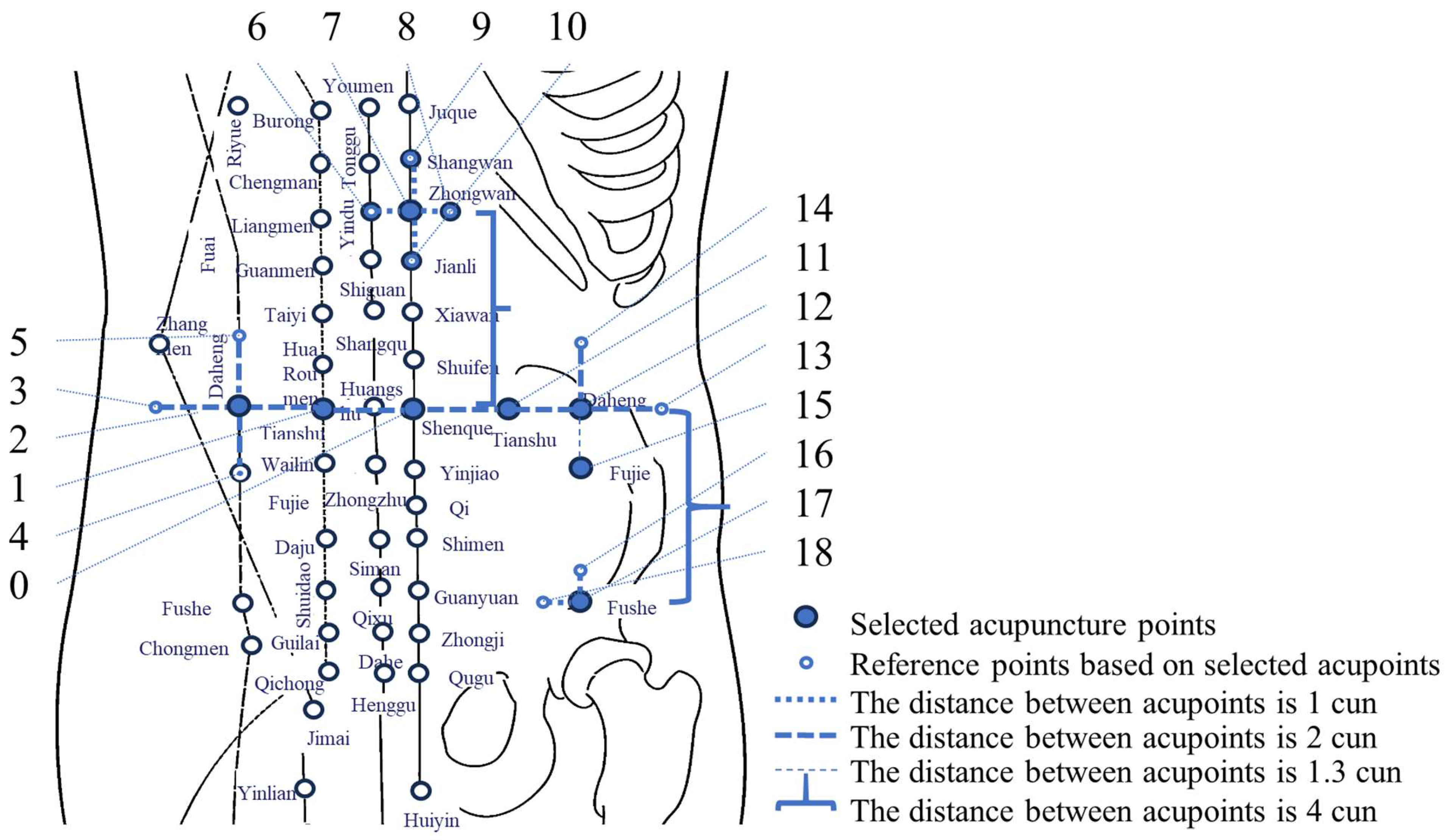
2.2. Key-Point Model for Abdominal Massage Action

The position of the colon in the abdomen cannot be artificially determined unless medical imaging technology is used, so the key-point model for abdominal massage action (see Figure 2) is used as the positioning basis for abdominal massage. The positioning basis is detailed in a paper by this team [23]. Based on the model, the team carried out the subsequent force-displacement data collection and analysis processing.

3. Abdominal Human Data Collection

3.1. Experimental Subjects

From September to December 2024, this study meticulously selected 12 healthy subjects based on strict inclusion and exclusion criteria. According to the classification standards of the World Health Organization (WHO) and China, underweight is defined as a BMI < 18.5, the normal BMI range is between 18.5 and 24, and overweight is defined as a BMI > 24. Based on the key indicator of body fat percentage, these 12 subjects were categorized into three body types: standard, underweight, and overweight. The specific classification details are provided in Table 1. The body fat percentage data used in this study were accurately collected using the Xiaomi Body Fat Scale, a device with high-precision measurement capabilities, ensuring the accuracy and reliability of the experimental data.

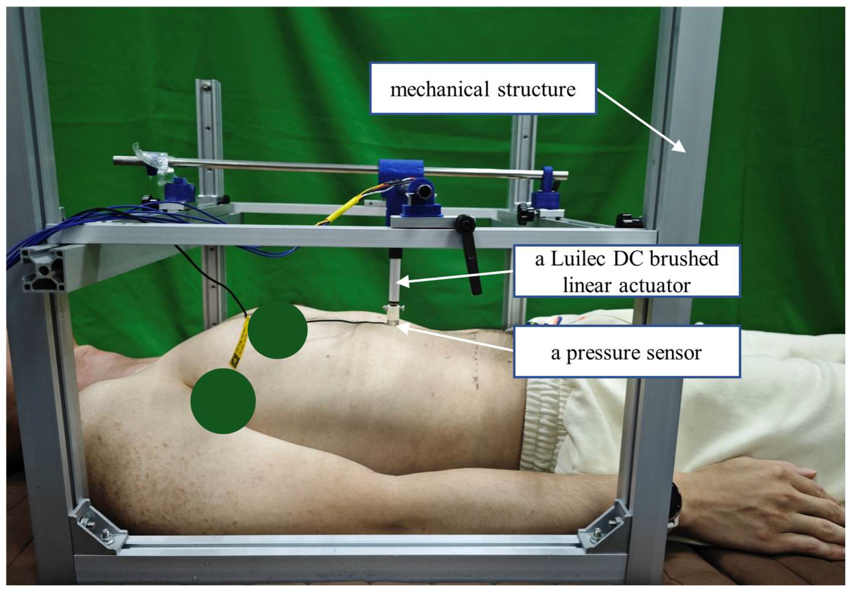
3.2. Experimental Equipment

This study utilized a Muscle Condition Quick Assessment System (OE220, Ito, Japan) and a self-developed mechanical testing platform (as shown in Figure 3). The self-developed mechanical testing platform includes the following components: the US-100 ultrasonic distance measurement module (Touglesy, Zhejiang, China), which enables precise distance measurement; a push-rod motor MNTL (Luilec, Changzhou, China, 50 mm stroke, 60 N load, 5 mm/s speed), providing stable power output for the experiment; a pressure sensor SBT674 (Sibatuo, Guangzhou, China. range: 0–20 N, sensitivity: 1.5 ± 10% mV/V), used to accurately measure pressure changes during the experiment; and the overall mechanical structure of the self-developed experiment platform. For data acquisition and processing, the Zhengdian Atomic Serial Port Debugging Assistant software (XCOM V2.6) was employed. This software features efficient data transmission and processing capabilities, enabling the real-time monitoring and analysis of experimental device data.

3.3. Experimental Protocol

The experimental protocol consists of two main parts, as detailed below:
Experiment 1: Preliminary Assessment of Maximum Displacement and Pressure at Key Action Points
This experiment aims to preliminarily determine the maximum displacement and pressure at key action points through manual operation. The results will establish safe pressing depth and pressure ranges for subsequent experiments, ensuring the experiments are conducted under safe conditions.
(1) Preparation Phase:
  • Conduct a questionnaire survey for each subject, recording details such as the time of their last bowel movement within the past 24 h, as well as basic physical metrics including height, weight, body fat percentage, waist width at the navel, abdominal thickness at the navel, and age.
  • Have the subject lie flat on a bed with their arms naturally resting at their sides.
  • Identify and mark all anatomical landmarks on the subject’s body. Measure the corresponding distances between these landmarks. Note: For female subjects, the distance between the nipples is not recorded.
  • Based on GB/T 23237-2009 “Human Measurement Methods for Acupoint Location,” [39] precisely calculate the positions of the action points and mark all identified points.
(2) Experimental Procedure:
  • The operator uses a muscle tension tester to locate the acupoints on the subject’s body.
  • Press perpendicularly to the body surface at a slow and steady pace.
  • Immediately stop pressing when the subject reports discomfort. Simultaneously, the ultrasonic distance sensor records the initial and final displacement data during the pressing process.
Experiment 2: Precise Recording of Force-Displacement Data at Key Action Points
This experiment builds on the safe pressing depth and pressure reference values determined in Experiment 1. It aims to precisely record force-displacement data at key action points, obtaining the force-displacement relationships at multiple abdominal points for each individual.
(1) Supplementary Survey:
  • Before conducting Experiment 2, administer a supplementary questionnaire to inquire whether the subject has had a bowel movement between Experiments 1 and 2.
(2) Preparation and Procedure:
  • Have the subject lie flat on the bed again, with their arms naturally resting at their sides.
  • Identify and mark all key action points.
  • The operator controls the action head of the self-developed mechanical testing platform, aligning it with the abdominal action points on the subject’s body.
  • The single reciprocating compression method is adopted. During a single reciprocating compression cycle, the actuator (a Luilec DC brushed linear actuator) of the mechanical experiment platform moves from a position where it does not touch the subject’s abdomen, presses into the abdomen to a target depth, and then retracts to a position where it no longer makes contact. The maximum pressing speed of the push rod motor is set to 5 mm/s, perpendicular to the surface of the abdomen. After each single reciprocating compression, data are recorded, and the target pressing depth of the push rod motor is increased by 5 mm for the next compression. This process continues until the pain threshold determined in Experiment 1 is reached. During the experiment, the pressing frequency of the push rod motor is up to 0.25 Hz, slowly acting on the human abdomen.
  • Throughout the experiment, monitor and record displacement and force sensor data in real-time. Output the data uniformly after the experiment concludes.
  • If the subject experiences discomfort during the experiment, stop immediately and record the data at that point. These data will provide critical support for subsequent safe force-displacement control.

4. Derivation Method and Results of the Variable Stiffness Physical Model for the Abdomen

Human soft tissues exhibit properties such as linearity, nonlinearity, viscoelasticity, and incompressibility. Traditional physical quantities in elasticity theory, such as Lamé constants, Young’s modulus, damping coefficients, and stress density, are insufficient to fully characterize these properties of soft tissues [40,41]. The research literature [42] indicates that the force-displacement relationship of soft tissues is nonlinear, which aligns with experimental results. Given that the experimental subjects can be categorized into three body types—underweight, standard, and overweight—based on BMI, this study selects one subject from each category through random sampling to derive the model.

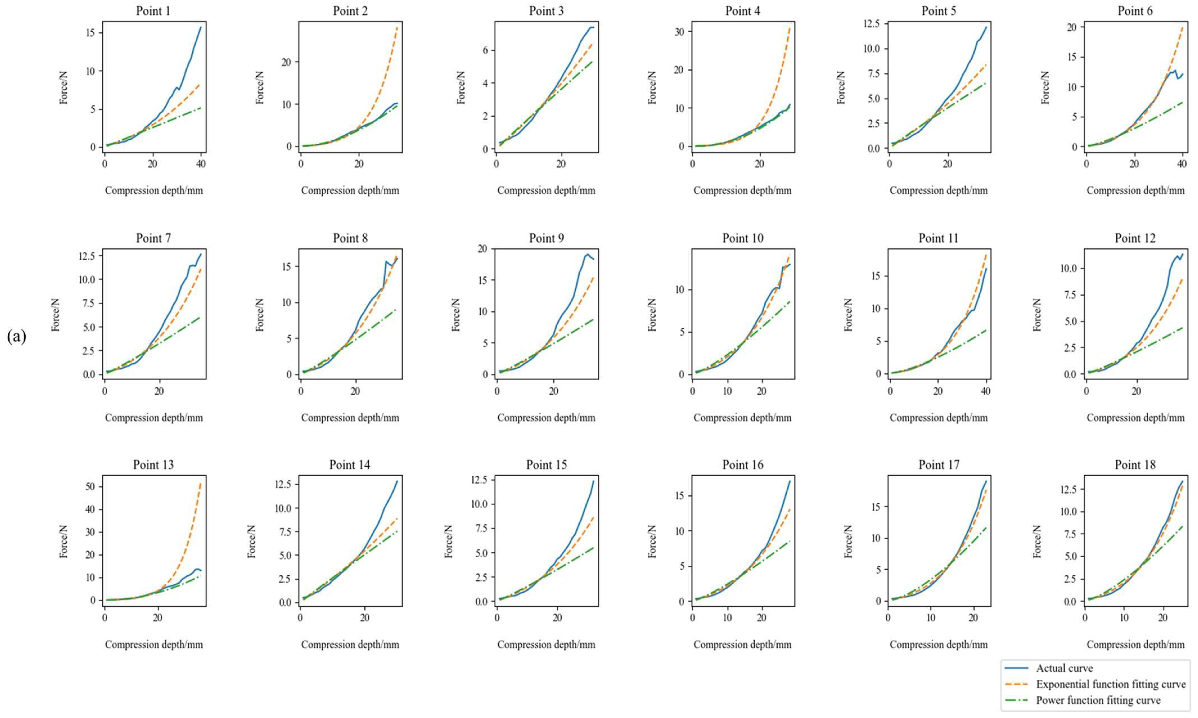
4.1. Variable Stiffness Physical Model Based on Exponential Function

Experimental results show that the force-displacement curve of human soft tissues approximates an exponential function. Additionally, due to the viscoelastic nature of soft tissues, the response during loading and unloading is not immediate but exhibits an exponential delay ( e t τ ) [43]. Therefore, this study defines the elastic coefficient k as an exponential function of the deformation x . The stiffness k in the deformation model can be expressed as follows:
k = a × e b x
Given that a and b are undetermined parameters and x represents the deformation at the pressed location. Since the pressing speed during abdominal massage is very low, the influence of pressing speed on the force can be neglected. By simplifying the soft tissue deformation model, the variable stiffness deformation model for soft tissues is established as follows:
F = k × x = a × e b x × x
Sum both sides logarithmically to obtain
ln F = ln a + ln x + b x
Let y = ln F ln x , A = ln a , B = b , then the formula is
y = A + B x
Define the loss function as mean squared error (MSE):
M S E = 1 N i = 1 N ( y i A + B x i ) 2
A physical model of soft tissue with variable stiffness was established based on the least squares method. The force level data of three subjects were randomly selected, and the values of parameters uppercase A and uppercase B were determined to minimize MSE. The partial derivative equation of the mean square error was established.
Find the partial derivative of uppercase A and uppercase B , and make it zero, and the solution parameters are obtained:
B = N i = 1 N x i y i i = 1 N x i i = 1 N y i N i = 1 N x i 2 i = 1 N x i 2 A = 1 N i = 1 N y i B 1 N i = 1 N x i
The simulation results of the variable stiffness physical model based on the exponential function representation (referred to as Model 1) are shown in Table 2 below. Figure 4 analyzes the fitting results of three typical body types based on Model 1 through five evaluation indicators.
The table data fitted by Model 1 presents the fitting results of all three types of points: the coefficients of the physical model and five fitting evaluation indicators: R_square (determination coefficient), MAPE (mean absolute percentage error), MSE (mean square error), RMSE (mean square error) and MAE (mean absolute error). R-square is mainly used to quantify the goodness of fit of a linear regression model to explain the proportion of variation in the response variable explained by variation in the independent variable. R-square values range from 0 to 1, with higher values indicating that the model can better explain the variation in the data. The two variable stiffness physical models involved in this article are both nonlinear models, which have been processed to become linear models, so R-square is suitable for use. MAE, MSE, RMSE, and MAPE are the key indexes in regression analysis. MAE ∈ [0, +∞]. The smaller the value of MAE, the better the precision of the prediction model. MSE ∈ [0, +∞]. MSE is a loss function, the smaller the value, the smaller the error. RMSE is the fitted standard deviation of the regression coefficients and is the square root of MSE, which is more intuitive in order of magnitude. MAPE ∈ [0, +∞], the smaller the value, the better the model fits.
Based on these five indicators, three types of fitting (standard, underweight, overweight) are analyzed:
R_square > 0.90 accounted for 80.77% (Standard type 88.89%, Underweight type 100%, Overweight type 52.94%), R_square > 0.95 accounted for 71.15% (Standard type 72.22%, Underweight type 100%, Overweight type 41.18%).
MAPE < 10% accounted for 25.00% (Standard type 5.56%, Underweight type 52.94%, Overweight type 17.65%), MAPE < 20% accounted for 75.00% (Standard type 77.78%, Underweight type 100%, Overweight type 47.06%), MAPE < 30% accounted for 90.38% (of which Standard type 94.44%, Overweight type 76.47%).
MSE: The Standard type is between 0.0081 and 1.2439, and the MSE is lower at most points, indicating a smaller fitting error. The Underweight type is between 0.0098 and 0.3865, and the MSE is lower at most points, indicating a smaller fitting error. The Overweight type is between 0.0005 and 2.3355, and the MSE is higher at some points, indicating a larger fitting error.
RMSE: Standard types range between 0.0902 and 1.1153, with a lower RMSE for most points, indicating a smaller difference between predicted value and actual value. Underweight types range between 0.0991 and 0.6217, with a lower RMSE for most points, indicating a smaller difference between predicted value and actual value. Overweight types range between 0.0005 and 2.3355, with a higher MSE for some points, indicating a larger fitting error.
MAE: Standard types range between 0.0570 and 0.6087, with a lower MAE for most points, indicating a smaller prediction error. Underweight types range between 0.0756 and 0.4201, with a lower MAE for most points, indicating a smaller prediction error. Overweight types range between 0.0181 and 0.8559, with a higher MAE for some points, indicating a larger prediction error.
Comprehensive comparison: The fitting effect is ranked as Underweight > Standard > Overweight; Error: The error of the Overweight type is significantly greater than that of Standard. Model explanatory power: Underweight and Standard type models have stronger explanatory power, while Overweight type models have weaker explanatory power.

4.2. Variable Stiffness Physical Model Based on Power Function Representation

Model 1 has a weak explanatory power for the Overweight type, so to take the Overweight type into account, this paper adds a discussion of the performance of other models. Since the pressing speed in abdominal massage is very low, the effect of massage speed on massage force is also ignored here.
Judging that the trend of the actual curve is similar to the exponential growth trend, the team found that the trend of the power function is similar, so a mathematical model of variable stiffness deformation of soft tissue is established in the form of a power model (Model 2):
F = c × x d
where c and d are both undetermined parameters, and x is the deformation when it is pressed.
Sum both sides logarithmically to obtain:
ln F = ln c + d ln x
Let Y = ln F , C = ln c , D = d , X = ln x , then, the formula is
Y = C + D X
Using the same least squares linear regression method, the results are shown in Table 3 below. Figure 5 analyzes the fitting results of three typical body types based on Model 2 through five evaluation indicators.
The Model 2 fitting results show the fitting of all three types of points:
R_square > 0.90 accounted for 63.46% (Standard type 33.33%, Underweight type 82.35%, Overweight type 76.47%), R_square > 0.95 accounted for 23.08% (Standard type 11.11%, Underweight type 11.76%, Overweight type 47.06%).
MAPE < 10% accounted for 7.69% (Standard type 0%, Underweight type 0%, Overweight type 23.53%), MAPE < 20% accounted for 59.62% (Standard type 29.41%, Underweight type 82.35%, Overweight type 70.59%), MAPE < 30% accounted for 90.38% (of which Standard type 83.33%, Underweight type 100%, Overweight type 88.24%).
MSE: The Standard type ranges between 0.0518 and 6.6155, with a higher MSE for some points (e.g., 6.6155 for Point 17), indicating a larger fitting error. The underweight type ranges between 0.0838 and 1.9354, with a lower MSE for most points, indicating a smaller fitting error. The overweight type ranges between 0.0032 and 0.6245, with a lower MSE for most points, indicating a smaller fitting error.
RMSE: Standard types range from 0.2275 to 2.5721, with a higher RMSE for some points (e.g., 2.5721 for Point 17), indicating a larger difference between the predicted value and actual value. Underweight types range from 0.2896 to 1.3912, with a lower RMSE for most points, indicating a smaller difference between predicted value and actual value. Overweight types range from 0.0564 to 0.7903, with a lower RMSE for most points, indicating a smaller difference between predicted value and actual value.
MAE: Standard types range between 0.1834 and 1.5820, with a higher MAE for some points (e.g., 1.5820 for Point 17), indicating a larger prediction error. Underweight types range between 0.1697 and 0.8928, with a lower MAE for most points, indicating a smaller prediction error. Overweight types range between 0.0467 and 0.5376, with a lower MAE for most points, indicating a smaller prediction error.
Comprehensive comparison: The fitting effect is ranked as Overweight > Underweight > Standard; Error: The error of the Standard type is significantly greater than that of the Underweight and Overweight types. Model explanatory power: Overweight and Underweight type models have stronger explanatory power, while Standard type models have weaker explanatory power.

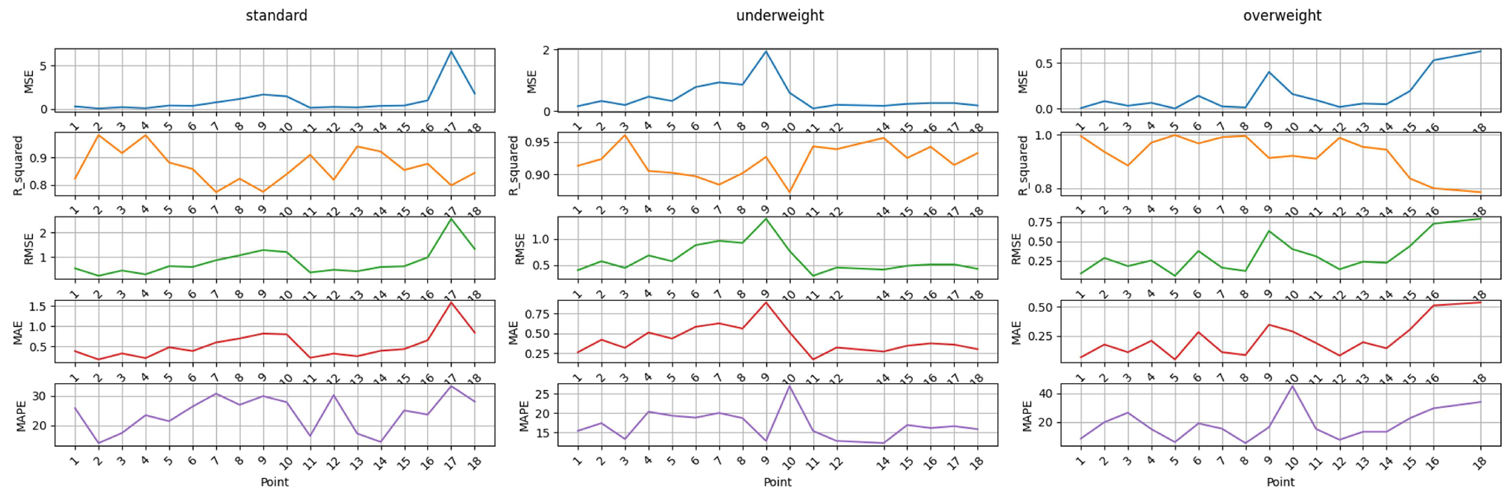
4.3. Comparison of Two Fitting Models

The two models are visually compared, as shown in Figure 6. Based on the comparison of the above five evaluation indicators, it can be concluded that Standard is suitable for selecting Model 1. The Overweight type is suitable for selecting Model 2. The Underweight type seems to perform well in both models, but Model 1 performs better. Therefore, for the three body types in the future, this paper chooses Standard and Underweight types to use Model 1, and Overweight types to use Model 2 to fit.
Use Python 3.11.0 to calculate the accuracy of the two models. Set the tolerance threshold to 0.6 N, and the result exceeding the tolerance threshold will be judged as an error, resulting in the results shown in Table 4.
It can be seen that in most cases, the overall performance of Model 1 is better than that of Model 2. But in the overweight type, the accuracy of Model 2 is higher. The accuracy rate is also related to the prediction range, and the accuracy rate decreases as the prediction range expands. Especially for the prediction of the whole data, the accuracy rate of only one reaches 50%. Focusing on the results of the 0–20 mm pressing depth stage, the accuracy rate of both standard and underweight types can reach more than 90%, and the overweight type needs to focus on 0–15 mm to achieve more than 90% accuracy.
The above results prove that the derivation of these two variable stiffness physical models has excellent application value for the prediction of massage force within a certain range. However, for the application of the full data range, the model needs to be further optimized to improve performance on a large range of data.

5. Abdominal Massage Force Prediction Algorithm Based on Machine Learning

The variable stiffness physical model derivation is based on the known force level data of the subject. For a new subject, receiving a tentative massage with a low output force of the robot is not an acceptable solution for everyone. To respect the subject’s autonomous wishes, this section proposes a pressure value prediction model based on Transformer architecture, which aims to accurately predict the pressure value. The model combines feature engineering, deep learning, and performance evaluation methods, and realizes efficient pressure value prediction through data preprocessing, model training, result visualization, and error analysis. The eigenvalues as input are shown in Table 5. The algorithm flow chart is shown in Figure 7, and the predicted abdominal massage interaction force result is the output. This is used as the robot’s massage force, thereby improving the safety of the robot massage.

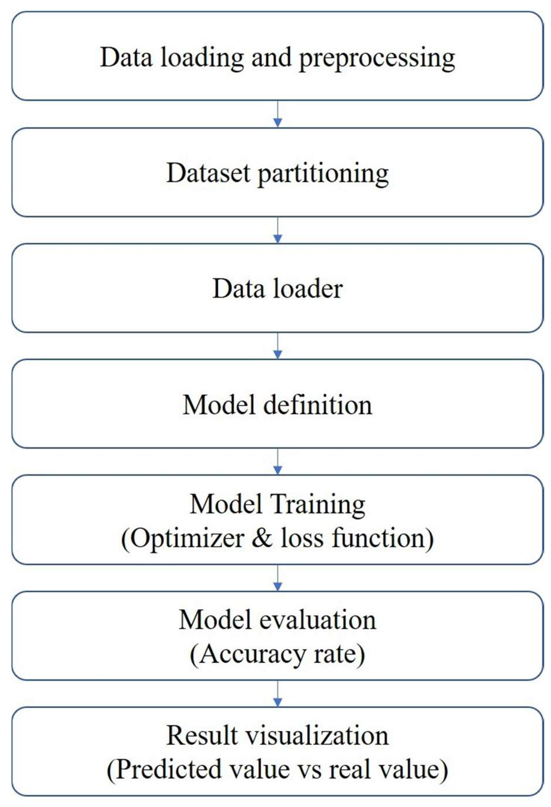
5.1. Algorithm Execution Process

  • Data loading and preprocessing
Read data from an Excel file, including continuous features (such as “press depth”) and discrete features (such as “points”), as well as target values (“pressure values”). Standardize continuous features and generate polynomial features (such as squares and cubes) to capture nonlinear relationships. Embed discrete features, mapping them to low-dimensional dense vectors. Stitch the processed features into feature matrices as input to the model.
2.
Dataset partitioning
Divide the data into a training dataset and a test set based on the ID column to ensure that data with different IDs do not appear in either the training dataset and the test set to avoid data leakage.
3.
Data loader
Use the PressureDataset class to encapsulate feature matrices and target values as PyTorch 2.6.0 Dataset objects. The dataset is divided into batches by the DataLoader, enabling efficient batch training and evaluation.
4.
Model definition
Model Architecture: Embedding Layer: Embedding id features, mapping them to 8-dimensional vectors; Encoder: Mapping input features to 128-dimensional space and nonlinear transformation using GELU activation function and layer normalization (LayerNorm); Transformer Encoder: Capturing complex relationships between features using a four-layer Transformer Encoder. Output Layer: Mapping the output of the Transformer to the final pressure value prediction.
5.
Model training
Model training using the AdamW optimizer and Huber loss function. In each training cycle (epoch): Forward propagation of the training dataset, calculation of predicted value, and loss. Update model parameters through backpropagation. Evaluate model performance on the test set, calculate test accuracy, and mean absolute error (MAE).
6.
Visualization of results
Use the plot_predictions function to plot the predicted value against the true value, distinguishing between samples with tolerable errors and those outside the tolerable range. Visualizations include statistics such as the perfect prediction line (diagonal), MAE, and accuracy.

5.2. Algorithm Complexity Analysis

  • Time complexity
Data preprocessing: The time complexity of normalization and polynomial feature generation is O n d , where n is the number of samples and d is the feature dimension. The time complexity of embedding operations is O n k , where k is the embedding dimension.
Model training: The time complexity of each training cycle is O b d + e · l , where b is the batch size, d is the input feature dimension, e is the embedding dimension. l is the number of layers of the Transformer encoder. The total training time complexity is O T · b d + e · l , where T is the number of training cycles. Model inference: The time complexity of a single inference is O d + e · l .
2.
Space complexity
Data Storage: The space complexity of the feature matrix is O n d . The space complexity of the embedding matrix is O m k , where m is the number of classes of discrete features. Model Parameters: The space complexity of the embedding layer is O m k . The space complexity of the encoder and transformer layers is O d + e · h + h 2 · l , where h is the hidden layer dimension. Training Process: The space complexity of each batch is O b · d + e · h .

5.3. Experiments and Results

It can be seen from the results that the algorithm can achieve 58.60% accuracy in the full data, 73.20% accuracy in the range of 0–20 mm, and 92.60% accuracy in the range of 0–15 mm under the condition of unknown subject force level data. The algorithm outperforms the prediction results of the variable stiffness physical model almost comprehensively. Table 6 shows a comparison of the accuracy rates of the algorithm applied under different ranges of pressing depths. Figure 8 shows the accuracy results for the pressing depths of full data, 0–20 mm, and 0–15 mm.

6. Discussion

This study focused on the key issue of abdominal massage interaction force prediction and carefully designed and strictly implemented the abdominal force position data collection experiment. Through a scientific and rigorous experimental process, two kinds of abdominal variable stiffness soft tissue physical models were successfully deduced, namely the model based on exponential function and power function, and their applicability differences in different body types were deeply analyzed. At the same time, a machine learning-based abdominal massage force prediction algorithm was developed. The algorithm does not distinguish between groups of people, but only uses the personal information of new subjects as the eigenvalue input to output the predictive force. These two research results, namely the variable stiffness physical model and the machine learning prediction algorithm, provide key theoretical and data support for the development of abdominal massage robots.
The variable stiffness physical model proposed in this study focuses on solving the core control parameter mapping problem in the dynamic interaction between the abdominal massage robot and the human abdomen—that is, the implementation decoupling relationship between the pressing depth and the target pressure. By simplifying the physical model to express the nonlinear relationship between the pressing depth and the pressing force, an analytical dynamic equation can be provided for robot massage control without the need for a complex abdominal biomechanics model simulation.
From the perspective of model construction and practical application effects, the variable stiffness physical model based on the exponential function and power function shows unique advantages in fitting the force-position relationship of abdominal soft tissue. Specifically, Model 1, based on the exponential function, is more suitable for standard and underweight body types, while Model 2, based on the power function, is more suitable for overweight body types. This phenomenon fully shows that there are significant differences in the mechanical properties of abdominal soft tissue in different body types, and targeted strategies must be adopted in the modeling process. In terms of experimental design and data collection, this study selected 12 volunteers with different body types to participate in the experiment. These volunteers covered a variety of physical characteristics, and the experimental protocol was carefully designed with high rigor, providing a reliable data basis for subsequent model derivation and algorithm construction.
Although there were only 12 subjects, approximately 18 action points were selected on the abdomen of each subject for mechanical data collection and analysis. According to the research conducted by our team during the same period, it was found that the thicknesses of various soft tissues in the body at each action point in the CT images corresponding to the subjects were inconsistent, so they could all be regarded as independent data. Therefore, the current sample size is equivalent to the mechanical data of 216 points. However, at present, the accuracy of these two kinds of abdominal variable stiffness soft tissue physical models in the full data prediction scenario is at a low level, which reveals that the model has a significant lack of generalization ability when dealing with complex and diverse actual data. Similarly, there are similar problems in the prediction algorithm based on machine learning. After analysis, the mechanical properties of human abdominal soft tissue are affected by many factors, including individual physiological differences, respiratory movement, etc., and current models and algorithms fail to fully consider these factors in the construction process. The sample size in the database is relatively limited. Currently, although the sample size consists of 12 people, each group of people is only represented by around 4 individuals. It is difficult to comprehensively and accurately represent the abdominal mechanical properties of all populations. To further improve the generality of the research results, follow-up studies can consider expanding the sample size to include more people of different ages, genders, and regions, as well as patients with different degrees of constipation or other abdominal diseases.
Future research can be carried out in the following two directions.
Longitudinal Deepening:
(A)
Enriching the Database: On the one hand, the impacts of factors such as different ages, regions, genders, and constipation durations on the abdominal interaction force and pressing depth should be considered. On the other hand, the impacts of massage tips of different sizes and shapes on the abdominal force and the subjective feelings of the subjects should be taken into account. We could expand the sample set to optimize the variable-stiffness physical model. We could introduce the quantitative modeling of subjective feelings, incorporate the subjective evaluations of subjects into the data, establish a database of the mapping relationship between “mechanical parameters–subjective feelings”, and extract personalized force control grading standards for light, medium, and heavy massage, to achieve the dynamic matching between voice instructions such as “increase the force” and “decrease the force” and force control parameters for the subsequent robots.
(B)
Enhancing the Generalization Ability of the Model: In view of the fitting limitations of the existing exponential/power functions, we could introduce polynomial functions, fractional-order differential equations, or neural network models (such as Long Short-term Memory (LSTM) time-series networks) to construct a hybrid model framework and improve the generalization ability of the physical model.
(C)
Complementing Dynamic Interaction Scenarios: We could develop a respiratory motion compensation algorithm and utilize visual technology to reduce the interference problem of abdominal displacement caused by breathing, thereby improving the accuracy of the prediction model.
Horizontal Expansion
(A)
Integration with the Intelligent Adaptive Control System. a. Model-driven control strategy: Embed the established variable-stiffness physical models (exponential/power functions) into the robot control system. Through the dynamic comparison between real-time force-displacement data and model prediction values, develop an adaptive algorithm based on model predictive control or impedance control to achieve the autonomous adjustment of massage force according to the change in tissue stiffness; b. Real-time force-feedback closed-loop: Establish a real-time communication interface between the robot’s end-effector and the database. Continuously update the prediction model parameters using the massage force prediction algorithm. Combine the feedback from the force sensor to achieve a “perception–decision–execution” closed-loop control, thereby enhancing the dynamic response ability to complex abdominal deformations.
(B)
Integration with the Digital Twin Model: Combine finite-element simulation (such as the Abaqus soft-tissue model) with medical imaging data to construct a “mechanics-tissue state” coupling model, use the finite element model simulation of the abdomen to construct a strain rate-dependent viscoelastic constitutive equation, to better describe the stress–strain effect generated when the abdomen is subjected to external force, and to enhance the prediction ability of abdominal mechanical response characteristics during the massage process.

7. Conclusions

This research has made important breakthroughs in the field of abdominal soft tissue and robot interaction. Based on the mechanical experimental platform developed by our team, an abdominal force-displacement database was established, two physical models of variable stiffness soft tissue were constructed, and personalized applicable population classification standards were established. For the scene of unknown force parameters, a prediction algorithm framework based on machine learning was proposed, which effectively solved the problem that the massage output force of unknown subjects at the beginning of abdominal massage could not be clarified. Future research will expand the dataset, enhance the generalization ability of the model through multi-model coupling optimization, and complement dynamic interaction scenarios. Horizontally, it will also expand applications, such as integrating with intelligent control systems or finite-element simulation models, to expand application scenarios. The research in this paper is expected to provide a reliable basis for interaction forces in non-invasive therapeutic interventions.

Author Contributions

Conceptualization, P.S.; methodology, S.L. and H.Y.; software, Z.L.; formal analysis, X.T. and Z.L.; investigation, X.T.; resources, H.Y.; writing—original draft preparation, X.T. and Z.L.; writing—review and editing, X.T.; visualization, X.T.; project administration, P.S.; funding acquisition, H.Y., P.S. and S.L. All authors have read and agreed to the published version of the manuscript.

Funding

This research was funded by the National Key R&D Program of China, grant number (2022YFB4703300).

Institutional Review Board Statement

Ethic Committee Name: Ethics Committee of Yixing Jiuru City Rehabilitation Hospital; Approval Code: 20221104A08; Approval Date: 4 November 2022.

Data Availability Statement

The data are available from the corresponding author upon reasonable request.

Acknowledgments

Thanks to the volunteers of the mechanical experiments for their participation and dedication.

Conflicts of Interest

The authors declare no conflicts of interest.

References

  1. Brenner, D.M.; Corsetti, M.; Drossman, D.; Tack, J.; Wald, A. Perceptions, Definitions, and Therapeutic Interventions for Occasional Constipation: A Rome Working Group Consensus Document. Clin. Gastroenterol. Hepatol. 2024, 22, 397–412. [Google Scholar] [CrossRef] [PubMed]
  2. Sharma, A.; Rao, S. Constipation: Pathophysiology and Current Therapeutic Approaches. In Gastrointestinal Pharmacology. Handbook of Experimental Pharmacology; Greenwood-Van Meerveld, B., Ed.; Springer: Cham, Switzerland, 2016; Volume 239. [Google Scholar] [CrossRef]
  3. Imran, A.; Whitehead, W.E.; Palsson, O.S.; Trnblom, H.; Magnus Simrén. An approach to the diagnosis and management of rome iv functional disorders of chronic constipation. Expert Rev. Gastroenterol. Hepatol. 2020, 14, 39–46. [Google Scholar]
  4. Zhang, X.; Li, Y.; Jiang, X.; Liu, J.; Fang, Y.; He, Z.; Cui, Q. The 99mTc-DTPA labeled solid meal was used to measure the gastric and small intestinal transit in constipation patients and evaluate its value in evaluating colonic transit in constipation patients. Chin. J. Gastroenterol. Hepatol. 2025, 34, 224–227. [Google Scholar]
  5. Yang, Z.; Wu, C.; Gao, J.; Bai, D.; Zhu, L.; Liu, R.; Liang, Y.; Wu, Q. Prevalence of Chronic Constipation in Chinese Adults:a Meta-analysis. Chin. Gen. Pract. 2021, 24, 2092–2097. [Google Scholar]
  6. Leng, Y.; Wei, W.; Tang, X. Expert Consensus on Diagnosis and Treatment of Constipation by Traditional Chinese Medicine (2024). J. Tradit. Chin. Med. 2025, 66, 321–328. [Google Scholar] [CrossRef]
  7. Jones, K.C.; Du, W. Development of a massage robot for medical therapy. In Proceedings of the 2003 IEEE/ASME International Conference on Advanced Intelligent Mechatronics (AIM), Kobe, Japan, 20–24 July 2003. [Google Scholar]
  8. Aitreat-About Emma. Available online: https://www.aitreat.com/about-emma (accessed on 6 March 2025).
  9. Kuka-Solutions Database. Available online: https://www.kuka.cn/zh-cn (accessed on 6 March 2025).
  10. Hou, P.; Han, L. Development of a home—Use back—Scrubbing and massage robot. Mach. Des. Res. 2009, 25, 101–105. [Google Scholar] [CrossRef]
  11. Jiao, C.B. Structural Analysis and Optimization of the LLR—1 Traditional Chinese Medicine Massage and Physical Therapy Robot. Master’s Thesis, Shandong Jianzhu University, Jinan, China, 2012. [Google Scholar]
  12. Kong, Y.X. Design and Research of a Hybrid Robot Based on Traditional Chinese Massage Techniques. Master’s Thesis, North University of China, Taiyuan, China, 2021. [Google Scholar] [CrossRef]
  13. Aubo-Robotic. Available online: https://www.aubo-robotics.cn/cases_m (accessed on 6 March 2025).
  14. Universal Robots. Available online: http://www.universal-robots.com/ (accessed on 6 March 2025).
  15. Mimidis, K.; Galinsky, D.; Rimon, E.; Papadopoulos, V.; Zicherman, Y.; Oreopoulos, D. Use of a device that applies external kneading—Like force on the abdomen for treatment of constipation. World J. Gastroenterol. 2005, 11, 5. [Google Scholar] [CrossRef]
  16. Mowoot. Available online: https://www.mowoot.com/en/product/mowoot-2/#moreinfo (accessed on 6 March 2025).
  17. Mcclurg, D.; Booth, L.; Herrero—Fresneda, I. Safety and efficacy of intermittent colonic exoperistalsis device to treat chronic constipation: A prospective multicentric clinical trial. Clin. Transl. Gastroenterol. 2020, 11, e00267. [Google Scholar] [CrossRef]
  18. Choi, Y.I.; Kim, K.O.; Chung, J.W.; Kim, Y.J.; Park, D.K. Effects of automatic abdominal massage device in treatment of chronic constipation patients: A prospective study. Dig. Dis. Sci. 2020, 66, 3105–3112. [Google Scholar] [CrossRef]
  19. Li, H.Y.; Zhao, H.; Gong, Z.K. Application of a novel intestinal massage device in stroke patients with constipation. Nurs. Res. 2018, 32, 636–638. [Google Scholar]
  20. Ning, P.F. A Nursing Massage Robot for Promoting Digestion. CN109498397A, 22 March 2019. [Google Scholar]
  21. Zhu, H.L. A Novel Abdominal Massage Device. CN202020731814, 7 May 2020. [Google Scholar]
  22. Gou, Y.Q.; Yang, L.X. An Abdominal Massage Device for Gastroenterology. CN211750916U, 27 October 2020. [Google Scholar]
  23. Tang, X.; Ping, S.; Luo, Z.; Yu, H. A Novel 6-DOF Multi-Technique Abdominal Massage Robot System: A New Solution for Relieving Constipation and an Exploration of Standardization. Electronics 2025, 14, 1123. [Google Scholar] [CrossRef]
  24. Cardoso, M.H.S. Experimental Study of the Human Anterolateral Abdominal Wall: Biomechanical Properties of Fascia and Muscles. Ph.D. Thesis, Universidade do Porto, Porto, Portugal, 2012. [Google Scholar]
  25. Assoul, N.; Flaud, P.; Chaouat, M.; Letourneur, D.; Bataille, I. Mechanical properties of rat thoracic and abdominal aortas. J. Biomech. 2008, 41, 2227–2236. [Google Scholar] [CrossRef] [PubMed]
  26. Wang, H. Research on the Mechanical Properties of Adipose Tissue and Its Influence on the Simulation of Thoraco—Abdominal Impact Injury. Master’s Thesis, Tianjin University of Science and Technology, Tianjin, China, 2021. [Google Scholar] [CrossRef]
  27. Tayebi, S.; Gutierrez, A.; Mohout, I.; Smets, E.; Wise, R.; Stiens, J.; Malbrain, M.L. A concise overview of non-invasive intra-abdominal pressure measurement techniques: From bench to bedside. J. Clin. Monit. Comput. 2021, 35, 51–70. [Google Scholar] [CrossRef]
  28. Leclerc, G.E.; Debernard, L.; Foucart, F.; Robert, L.; Pelletier, K.M.; Charleux, F.; Ehman, R.; Tho, M.-C.H.B.; Bensamoun, S.F. Characterization of a hyper—Viscoelastic phantom mimicking biological soft tissue using an abdominal pneumatic driver with magnetic resonance elastography (MRE). J. Biomech. 2012, 45, 952–957. [Google Scholar] [CrossRef] [PubMed]
  29. Li, F.T.; Sun, L.F.; Tao, Y.P.; Yang, P.; Ji, M.Q.; Sang, J.B. Inversion of constitutive parameters of plantar soft tissue using random forest and neural networks algorithms. Med. Biomech. 2024, 39, 476–481. [Google Scholar]
  30. Remus, R.; Sure, C.; Selkmann, S.; Uttich, E.; Bender, B. Soft tissue material properties based on human abdominal in vivo macroindenter measurements. Front. Bioeng. Biotechnol. 2024, 12, 1384062. [Google Scholar] [CrossRef]
  31. Zheng, Y.; Ning, H.; Rangarajan, E.; Merali, A.; Geale, A.; Lindenroth, L.; Xu, Z.; Wang, W.; Kruse, P.; Morris, S.; et al. Design of a Cost-Effective Ultrasound Force Sensor and Force Control System for Robotic Extra-Body Ultrasound Imaging. Sensors 2025, 25, 468. [Google Scholar] [CrossRef]
  32. Kim, J.; Ahn, B.; De, S.; Srinivasan, M.A. An efficient soft tissue characterization algorithm from in vivo indentation experiments for medical simulation. Int. J. Med. Robot. Comput. Assist. Surg. 2010, 4, 277–285. [Google Scholar] [CrossRef]
  33. Robinson, D.G. The Dynamic Response of the Seated Human to Mechanical Shock. Ph.D. Thesis, Simon Fraser University, Burnaby, BC, Canada, 1999. [Google Scholar]
  34. Lim, Y.J.; Deo, D.; Singh, T.P.; Jones, D.B.; De, S. In situ measurement and modeling of biomechanical response of human cadaveric soft tissues for physics—Based surgical simulation. Surg. Endosc. 2009, 23, 1298–1307. [Google Scholar] [CrossRef]
  35. Shao, Y.; Zou, D.; Li, Z.; Wan, L.; Qin, Z.; Liu, N.; Zhang, J.; Zhong, L.; Chen, Y. Blunt liver injury with intact ribs under impacts on the abdomen: A biomechanical investigation. PLoS ONE 2013, 8, e52366. [Google Scholar] [CrossRef]
  36. Lan, F.C.; Cai, Z.H.; Chen, J.Q.; Ma, Z.W. Biomechanical Responses and Injury Evaluation of Human Thorax and Abdomen During Vehicle Collision. J. South China Univ. Technol. (Nat. Sci. Ed.) 2012, 40, 70–78. [Google Scholar]
  37. Du, T. Research on the Impact Biomechanics Response and Injury Evaluation of the Thorax of Automobile Occupants Covering the Liver. South China University of Technology. Ph.D. Thesis, Guangzhou, China, 2018. [Google Scholar]
  38. Hu, H.; Li, X.; Ding, L.; Zhao, C. Establishment of a Finite Element Model of the Thorax and Abdomen and Analysis of Collision Biomechanics. Stand. Sci. 2015, 7, 15–18+44. [Google Scholar] [CrossRef]
  39. GB/T 23237-2009; Methods of Anthropometry for Locating Acupuncture Points. China Standards Press: Beijing, China, 2009.
  40. Maurel, W.; Wu, Y.; Thalmann, N.M.; Thalmann, D. Biomechanical Models for Soft Tissue Simulation; Springer: Berlin/Heidelberg, Germany, 1998; pp. 23–25. [Google Scholar]
  41. Xu, S.P.; Liu, X.P.; Zhang, H.; Luo, J. Research progress on real—Time deformation models of soft tissues in virtual surgery. J. Biomed. Eng. 2010, 27, 435–439. [Google Scholar]
  42. Zhang, Q.K.; Luo, L.M.; Yang, W. Nonlinear model for real—Time simulation of soft tissue deformation. J. Appl. Sci. 2007, 25, 276–282. [Google Scholar]
  43. Jiang, C.T. Research on the Elastic Model of Human Soft Tissues. Master’s Thesis, Southeast University, Dhaka, Bangladesh, 2004. [Google Scholar]
Figure 1. Flowchart of the research scheme.
Machines 13 00441 g001
Figure 2. Model of key action points [23].
Machines 13 00441 g002
Figure 3. Self-developed mechanical experiment platform.
Machines 13 00441 g003
Figure 4. Analysis of five evaluation indicators of the fitting results of three types of typical body types based on Model 1.
Machines 13 00441 g004
Figure 5. Analysis of five evaluation indicators of the fitting results of three types of typical body types based on Model 2.
Machines 13 00441 g005
Figure 6. Comparison of the fitting effect of the two models of (a) standard, (b) underweight, and (c) overweight with the actual curve.
Machines 13 00441 g006aMachines 13 00441 g006b
Figure 7. Algorithm flow chart.
Machines 13 00441 g007
Figure 8. Accuracy results of (a) full data, (b) 0–20 mm, (c) 0–15 mm.
Machines 13 00441 g008
Table 1. Basic information of subjects.
Subject IDBody TypeBMIAge GroupGender
1Underweight17.630–40Female
2Underweight16.720–30Female
3Underweight17.520–30Female
4Underweight18.420–30Male
5Overweight25.520–30Male
6Overweight24.4<20Male
7Overweight24.930–40Male
8Standard21.230–40Female
9Standard2120–30Female
10Standard23.620–30Female
11Standard23.930–40Male
12Standard22.6<20Male
Table 2. Fitting results of Model 1.
PointabMSER_SquareRMSEMAEMAPE
standard1 0.1004 0.0183 0.1054 0.9347 0.3246 0.2604 20.9452
2 0.0302 0.1011 0.2988 0.8963 0.5466 0.3162 14.7593
3 0.1659 0.0087 0.0660 0.9721 0.2569 0.2097 13.5855
4 0.0175 0.1418 1.2439 0.7224 1.1153 0.6087 30.1429
5 0.1864 0.0093 0.1430 0.9565 0.3781 0.3215 16.9908
6 0.0650 0.0508 0.0346 0.9860 0.1860 0.1411 13.7449
7 0.0997 0.0330 0.2318 0.9298 0.4815 0.3619 21.8757
8 0.1433 0.0343 0.2687 0.9582 0.5184 0.3492 17.4046
9 0.1539 0.0318 0.5055 0.9308 0.7110 0.4662 20.6267
10 0.1209 0.0509 0.1835 0.9795 0.4284 0.3207 15.5394
11 0.0452 0.0579 0.0081 0.9944 0.0902 0.0570 4.8663
12 0.0611 0.0358 0.0474 0.9618 0.2176 0.1648 19.4340
13 0.0179 0.1220 0.1209 0.9579 0.3477 0.1915 14.9959
14 0.2327 0.0080 0.1368 0.9693 0.3698 0.2576 11.0203
15 0.1039 0.0297 0.0864 0.9671 0.2940 0.2309 16.5623
16 0.1410 0.0427 0.1090 0.9862 0.3302 0.2413 12.7977
17 0.1282 0.0778 0.4326 0.9868 0.6577 0.4582 14.7612
18 0.1082 0.0624 0.1181 0.9895 0.3437 0.2525 13.2991
underweight1 0.0589 0.0341 0.0164 0.9910 0.1280 0.0939 6.7222
2 0.1732 0.0097 0.0834 0.9803 0.2888 0.2231 12.2858
3 0.1579 0.0177 0.0163 0.9967 0.1278 0.1078 7.4928
4 0.1618 0.0144 0.1159 0.9764 0.3404 0.2771 13.6856
5 0.1634 0.0064 0.1098 0.9670 0.3313 0.2697 14.8614
6 0.1018 0.0398 0.0733 0.9903 0.2708 0.2104 8.8662
7 0.0959 0.0431 0.0716 0.9910 0.2676 0.2005 8.5638
8 0.1154 0.0382 0.0789 0.9909 0.2808 0.1882 9.5939
9 0.3083 0.0225 0.3865 0.9853 0.6217 0.4201 7.0918
10 0.0627 0.0492 0.0435 0.9906 0.2086 0.1786 15.6618
11 0.0233 0.0693 0.0168 0.9885 0.1295 0.0802 10.9623
12 0.2055 −0.0012 0.1001 0.9694 0.3164 0.2447 11.4228
14 0.0839 0.0370 0.0098 0.9974 0.0991 0.0756 6.1102
15 0.1442 0.0107 0.0561 0.9819 0.2368 0.1808 11.7923
16 0.1570 0.0154 0.0355 0.9921 0.1883 0.1546 9.8284
17 0.1272 0.0142 0.0669 0.9778 0.2586 0.1989 11.6283
18 0.1043 0.0205 0.0231 0.9913 0.1521 0.1196 8.7519
overweight1 0.0219 0.1113 0.2893 0.8053 0.5378 0.3175 22.2520
2 0.0143 0.1216 0.0603 0.9532 0.2455 0.1378 11.0655
3 0.0197 0.0633 0.0013 0.9953 0.0364 0.0304 15.3565
4 0.0752 0.0524 0.0462 0.9789 0.2150 0.1423 8.6169
5 0.0320 0.1010 0.2505 0.8911 0.5005 0.2917 21.2097
6 0.0345 0.1111 0.5196 0.8808 0.7209 0.4042 13.9233
7 0.0125 0.1561 0.8696 0.6874 0.9325 0.4799 30.5411
8 0.0294 0.1147 0.6115 0.8014 0.7820 0.4543 24.0232
9 0.0309 0.1290 2.3355 0.4953 1.5283 0.8559 49.3368
10 0.0058 0.1846 0.7322 0.6379 0.8557 0.4323 32.1401
11 0.0316 0.0723 0.0032 0.9970 0.0566 0.0465 6.8349
12 0.0203 0.1200 0.4308 0.7512 0.6564 0.3661 31.9549
13 0.1418 0.0056 0.0218 0.9825 0.1476 0.1269 10.9313
14 0.0387 0.0601 0.0005 0.9995 0.0219 0.0181 4.2279
15 0.0771 0.0268 0.0652 0.9450 0.2554 0.1932 16.9639
16 0.0994 0.0329 0.1472 0.9444 0.3836 0.2931 20.0819
18 0.0702 0.0521 0.1122 0.9616 0.3350 0.2569 20.3195
Table 3. Fitting results of Model 2.
PointcdMSER_SquaredRMSEMAEMAPE
standard10.12101.01470.28650.82230.53530.387025.8445
20.01561.83410.05180.98200.22750.183413.8429
30.19560.97330.19870.91610.44570.332417.3393
40.00722.15640.08160.98180.28560.217623.4146
50.22870.95840.38910.88150.62380.481921.3691
60.06151.29680.35060.85790.59210.391026.3764
70.11431.11550.75080.77270.86650.600930.7987
80.15761.14061.14290.82201.06910.697526.9581
90.17971.10061.65110.77411.28500.819329.9418
100.11651.28901.44660.83851.20270.800327.8771
110.03541.41850.13190.90940.36320.225616.3205
120.06821.14210.22590.81810.47520.328430.2806
130.00822.00310.17160.94020.41430.263517.1454
140.26780.98010.34890.92170.59070.396514.2547
150.11421.11650.38370.85380.61940.438425.0321
160.13831.23670.97360.87680.98670.656123.6336
170.10771.49376.61550.79772.57211.582033.3749
180.09651.38481.76580.84351.32880.842228.0752
underweight10.05041.26840.15910.91300.39890.262115.4010
20.20110.99600.32530.92330.57030.419617.3723
30.15781.10620.19510.96010.44170.317113.2735
40.18301.03530.46670.90490.68320.512220.3224
50.20170.95120.32560.90220.57060.434219.3071
60.08481.31390.77680.89680.88140.583518.8015
70.08001.33240.92840.88390.96350.627620.0087
80.09781.29680.85620.90150.92530.561718.6840
90.29331.15501.93540.92661.39120.892812.7703
100.05121.37770.59320.87240.77020.515326.9514
110.01341.64250.08380.94270.28960.169715.3725
120.25400.90570.20130.93840.44870.321212.7762
140.06401.33270.16860.95580.41060.270312.2073
150.16491.00880.23270.92490.48240.343716.8887
160.16781.06460.25930.94220.50920.374316.1239
170.13851.04960.25860.91410.50850.358216.5999
180.10521.11870.17990.93250.42420.299915.8232
overweight10.01031.92130.00750.99500.08640.06578.4288
20.00771.91730.08230.93620.28680.175219.8938
30.01741.38650.03260.88530.18060.109226.5079
40.06121.36690.06430.97060.25360.208115.0075
50.01581.84780.00320.99860.05640.04675.9198
60.01891.85380.14100.96770.37540.282519.0025
70.00472.26080.02600.99070.16120.109715.3694
80.01311.96680.01410.99540.11850.08515.2082
90.01032.17060.40040.91350.63270.345516.3824
100.00232.38900.15940.92120.39920.288245.1130
110.02231.53660.09460.91050.30760.188515.1905
120.00812.04050.01970.98860.14040.08087.5740
130.16000.97420.05670.95440.23810.195413.1718
140.02901.44430.04960.94460.22260.143313.1665
150.08451.09880.19340.83690.43980.304922.7294
160.11381.11010.52780.80070.72650.511029.6168
180.07381.24950.62450.78630.79030.537633.9833
Table 4. Comparison of the accuracy rates of the two models.
TypeCalculation RangeModel 1Model 2
standard0–1594.44%82.96%
0–2090.56%72.22%
full data46.03%35.85%
underweight0–1592.59%82.22%
0–2092.22%84.17%
full data55.43%40.25%
overweight0–1588.52%92.96%
0–2083.33%84.44%
full data42.99%45.90%
Table 5. Input and output of algorithms.
Feature
InputGender
Subjective Perception: Fear of Pain or Not
Subjective Perception: Sensitivity to Tickling or Not
Action Point
Body Fat Percentage.
Average Distance of “one cun”
Abdominal Thickness (over the navel)
Waist Width (over the navel)
Weight
BMI
Pressing Depth
OutputThe predicted value of the massage force
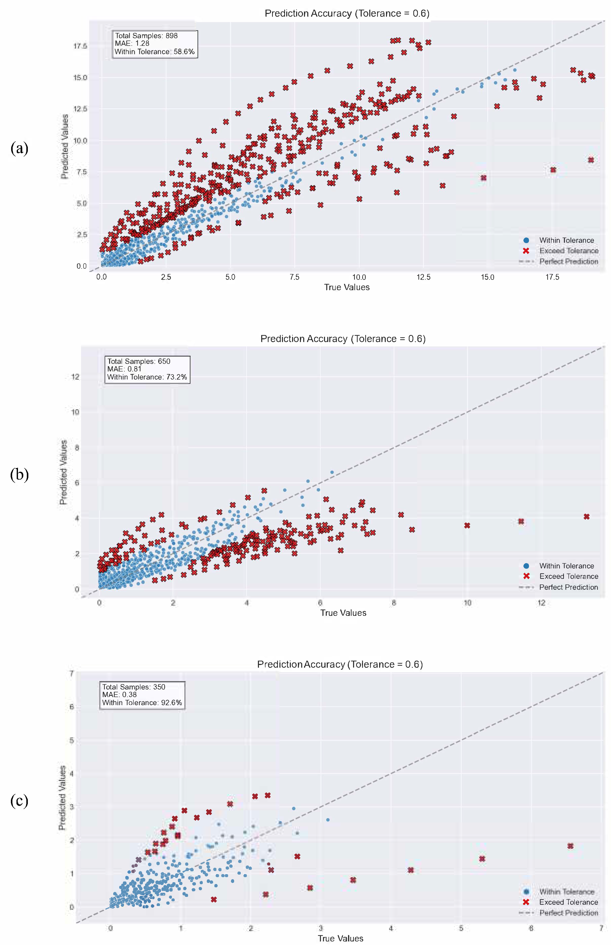
Table 6. Comparison of the accuracy of algorithms in different calculation ranges.
Calculation RangeAccuracy
0–1592.60%
0–2073.20%
full data58.60%
Disclaimer/Publisher’s Note: The statements, opinions and data contained in all publications are solely those of the individual author(s) and contributor(s) and not of MDPI and/or the editor(s). MDPI and/or the editor(s) disclaim responsibility for any injury to people or property resulting from any ideas, methods, instructions or products referred to in the content.

