
UAV Real-Time Target Detection and Tracking Algorithm Based on Improved KCF and YOLOv5s_MSES


Abstract
1. Introduction
- Based on some existent search strategies, this work initially proposes a new spatio-temporal search strategy (STS), which can comprehensively integrate the information of time and space to dynamically capture the target changes by incorporating historical data while retaining spatial information. Then, different from the traditional ones, the proposed STS can more effectively preserve the valuable feature information of the target, mitigate the target drift issues induced by the boundary effect, and efficiently enhance the search accuracy.
- This work innovatively puts forward an anti-loss strategy for target retracking (TR) based on the YOLOv5s_MSES algorithm. Such a strategy firstly utilizes the APCE to decide whether the tracking target will be obscured or out of the view field, and if so, the YOLOv5s_MSES is exploited to redetect all similar targets. Then, the APCE is further used to determine the real tracking target and track it again by resorting to the KCF algorithm. Thus, our TR strategy not only solves the problem that the current CF algorithm cannot retrack the lost target, but also facilitates the enhancement of tracking accuracy.
- In order to solve the issue of the fixed scale induced by the KCF algorithm, this work introduces an adaptive scale box method (ASB), enabling the dynamic adjustment of the scale of the target tracking box, which can improve the accuracy and stability for our derived algorithm, particularly in the case of large size variation.
2. Related Work
2.1. Boundary Effects
2.2. Tracking Loss
3. Methods
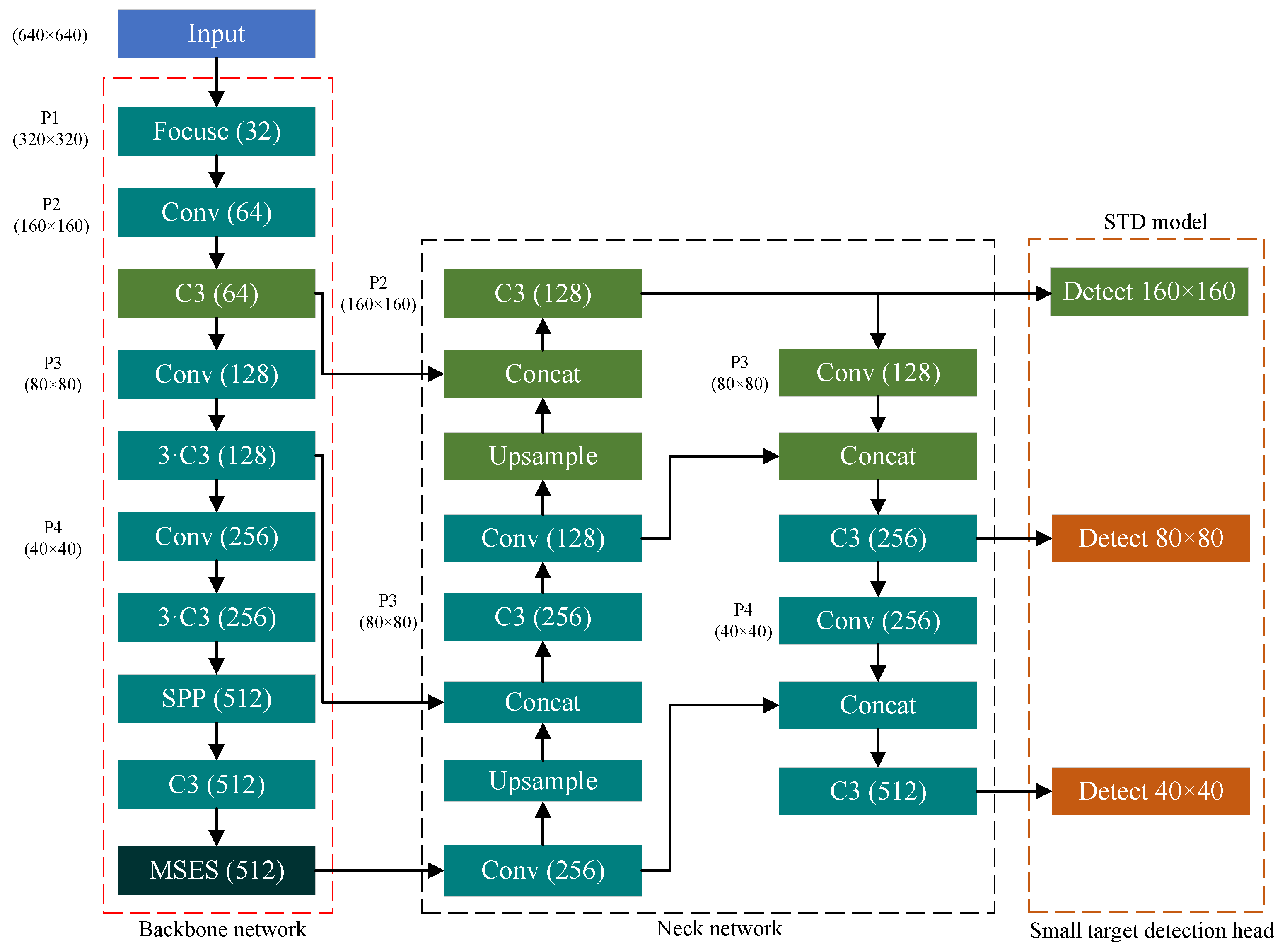
3.1. YOLOv5s_MSES Target Detection Algorithm
3.2. KCF Target Tracking Algorithm
3.3. Spatio-Temporal Search Strategy
3.4. Retracking Strategy for Target Loss
3.5. Adaptive Scale Box
4. Experiment
4.1. Experimental Data and Parameter Setting
4.2. The Ablation Experiments on OTB100 Dataset
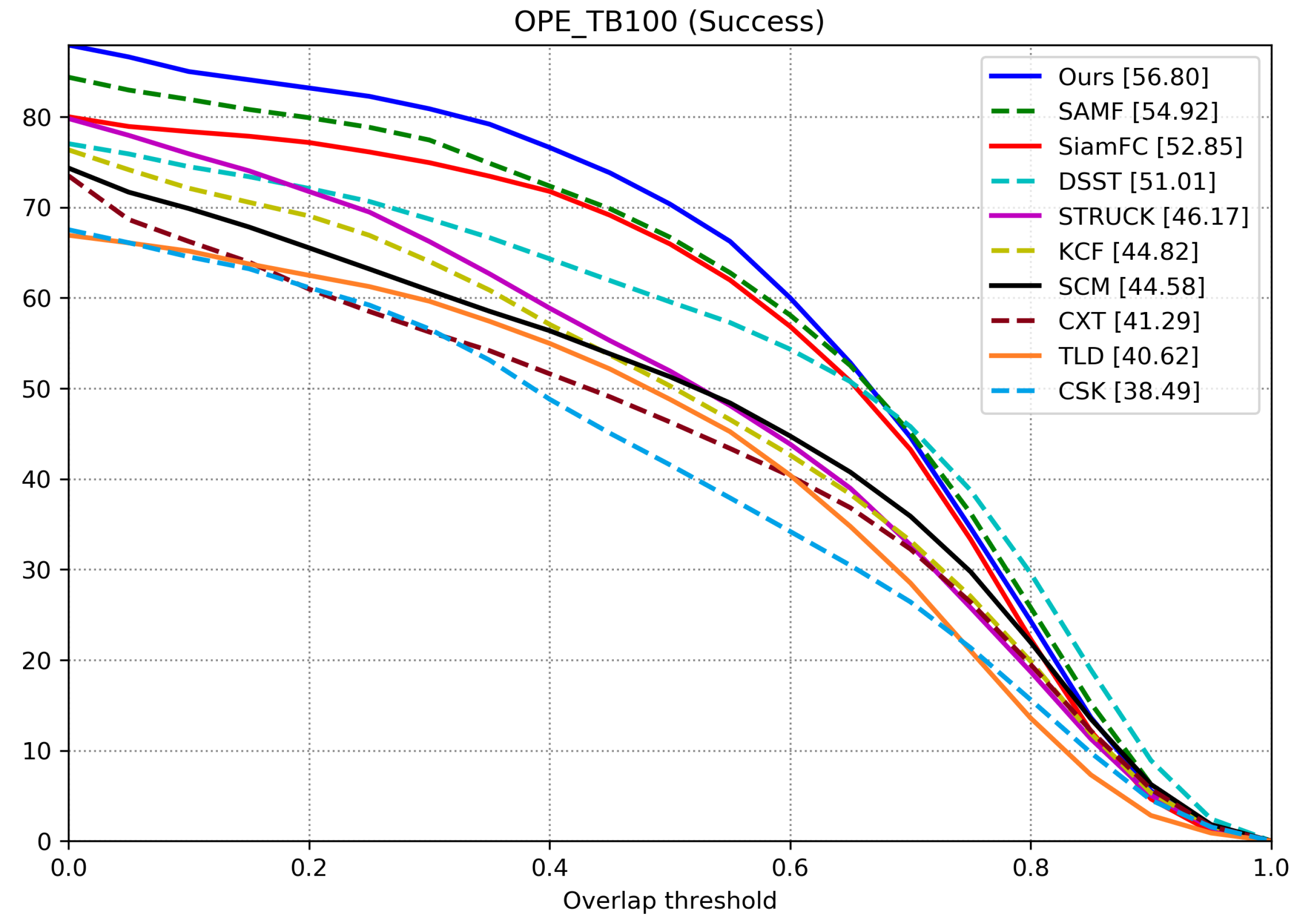
4.3. Contrast Experiments on the OTB100 Dataset
4.4. Contrast Experiments on the and Parameters
4.5. Contrast Experiments on the Parameter
4.6. Experiments on UAV123 Dataset
4.7. Comprehensive Performance Comparison
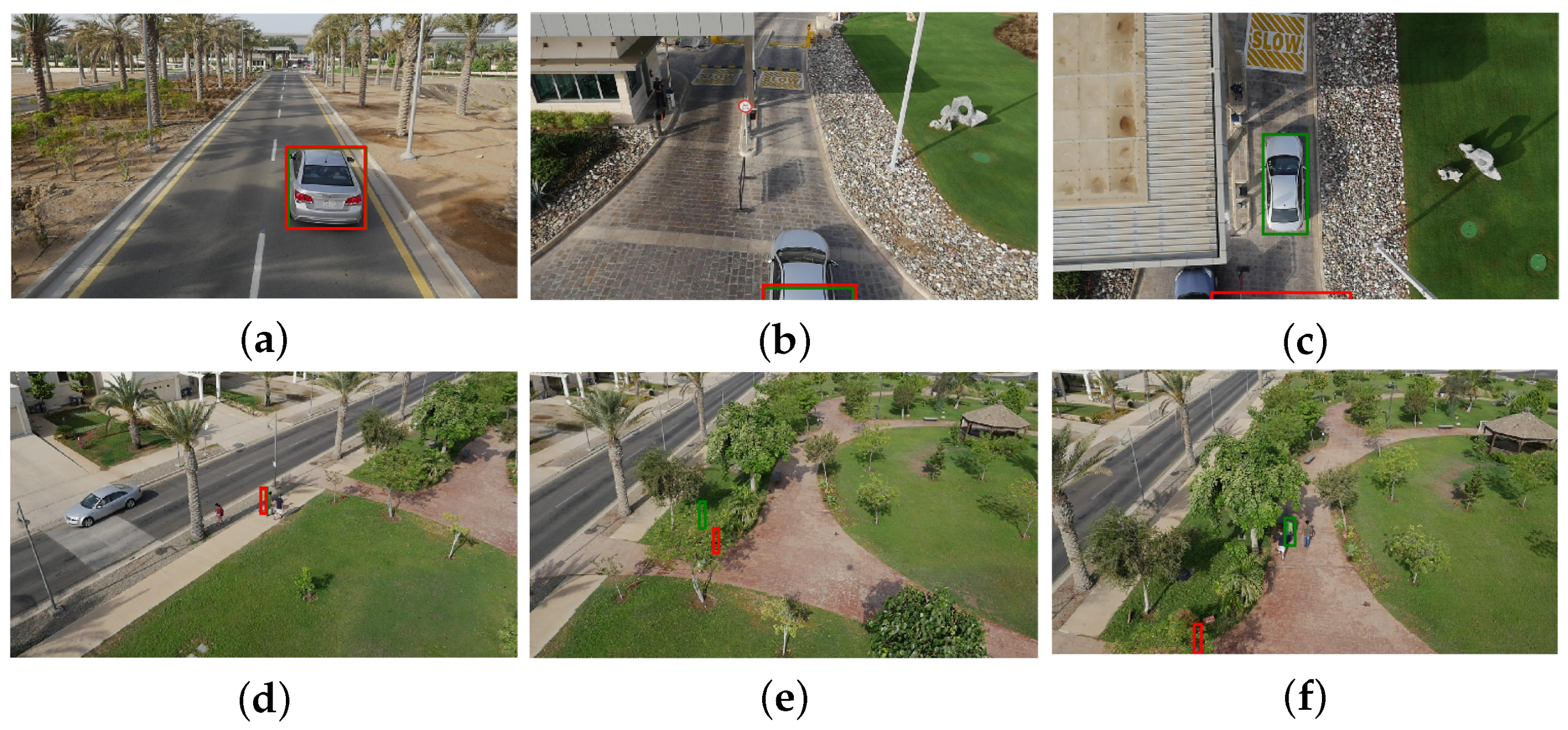
4.8. Experimental Effect and Analysis
5. Conclusions
Author Contributions
Funding
Institutional Review Board Statement
Informed Consent Statement
Data Availability Statement
Conflicts of Interest
References
- Yan, B.; Paolini, E.; Xu, L.; Lu, H. A target detection and tracking method for multiple radar systems. IEEE Trans. Geosci. Remote Sens. 2022, 60, 1–21. [Google Scholar] [CrossRef]
- Fang, H.; Liao, G.; Liu, Y.; Zeng, C. Shadow-assisted moving target tracking based on multi-discriminant correlation filters network in video SAR. IEEE Geosci. Remote Sens. Lett. 2023, 20, 1–5. [Google Scholar]
- Lee, M.; Lin, C. Object tracking for an autonomous unmanned surface vehicle. Machines 2022, 10, 378. [Google Scholar] [CrossRef]
- Hayat, M.; Ali, A.; Khan, B.; Mehmood, K.; Ullah, K.; Amir, M. An improved spatial–temporal regularization method for visual object tracking. Signal Image Video Process. 2024, 18, 2065–2077. [Google Scholar] [CrossRef]
- Song, P.; Li, P.; Dai, L.; Wang, T.; Chen, Z. Boosting R-CNN: Reweighting R-CNN samples by RPN’s error for underwater object detection. Neurocomputing 2023, 530, 150–164. [Google Scholar] [CrossRef]
- Zhang, R.; Shao, Z.; Huang, X.; Wang, J.; Wang, Y.; Li, D. Adaptive dense pyramid network for object detection in UAV imagery. Neurocomputing 2022, 489, 377–389. [Google Scholar] [CrossRef]
- Wang, J.; Meng, C.; Deng, C.; Wang, Y. Learning convolutional self-attention module for unmanned aerial vehicle tracking. Signal Image Video Process. 2023, 17, 2323–2331. [Google Scholar] [CrossRef]
- Wang, H.; Qi, L.; Qu, H.; Ma, W.; Yuan, W.; Hao, W. End-to-end wavelet block feature purification network for efficient and effective UAV object tracking. J. Vis. Commun. Image Represent. 2023, 97, 103950. [Google Scholar] [CrossRef]
- Daramouskas, I.; Meimetis, D.; Patrinopoulou, N.; Lappas, V.; Kostopoulos, V. Camera-based local and global target detection, tracking, and localization techniques for UAVs. Machines 2023, 11, 315. [Google Scholar] [CrossRef]
- Fu, C.; Li, B.; Ding, F.; Lin, F.; Lu, G. Correlation filters for unmanned aerial vehicle-based aerial tracking: A review and experimental evaluation. IEEE Geosci. Remote Sens. Mag. 2021, 10, 125–160. [Google Scholar] [CrossRef]
- Zhang, F.; Ma, S.; Qiu, Z.; Qi, T. Learning target-aware background-suppressed correlation filters with dual regression for real-time UAV tracking. Signal Process. 2022, 191, 108352. [Google Scholar] [CrossRef]
- Li, S.; Liu, Y.; Zhao, Q.; Feng, Z. Learning residue-aware correlation filters and refining scale for real-time UAV tracking. Pattern Recognit. 2022, 127, 108614. [Google Scholar] [CrossRef]
- Bolme, D.; Beveridge, J.; Draper, B.; Lui, Y. Visual object tracking using adaptive correlation filters. In Proceedings of the 2010 IEEE Computer Society Conference on Computer Vision and Pattern Recognition, San Francisco, CA, USA, 13–18 June 2010; pp. 2544–2550. [Google Scholar]
- Henriques, J.; Caseiro, R.; Martins, P.; Batista, J. High-speed tracking with kernelized correlation filters. IEEE Trans. Pattern Anal. Mach. Intell. 2014, 37, 583–596. [Google Scholar] [CrossRef] [PubMed]
- Danelljan, M.; Hager, G.; Shahbaz Khan, F.; Felsberg, M. Learning spatially regularized correlation filters for visual tracking. In Proceedings of the IEEE International Conference on Computer Vision, Santiago, Chile, 7–13 December 2015; pp. 4310–4318. [Google Scholar]
- Danelljan, M.; Hager, G.; Khan, F.; Felsberg, M. Accurate scale estimation for robust visual tracking. In Proceedings of the British Machine Vision Conference, Nottingham, UK, 1–5 September 2014. [Google Scholar]
- Bertinetto, L.; Valmadre, J.; Golodetz, S.; Miksik, O.; Torr, P.H. Staple: Complementary learners for real-time tracking. In Proceedings of the IEEE Conference on Computer Vision and Pattern Recognition, Las Vegas, NV, USA, 27–30 June 2016; pp. 1401–1409. [Google Scholar]
- Danelljan, M.; Shahbaz Khan, F.; Felsberg, M.; Van de Weijer, J. Adaptive color attributes for real-time visual tracking. In Proceedings of the IEEE Conference on Computer Vision and Pattern Recognition, Columbus, OH, USA, 23–28 June 2014; pp. 1090–1097. [Google Scholar]
- Lukezic, A.; Vojir, T.; Cehovin Zajc, L.; Matas, J.; Kristan, M. Discriminative correlation filter with channel and spatial reliability. In Proceedings of the IEEE Conference on Computer Vision and Pattern Recognition, Honolulu, HI, USA, 21–26 July 2017; pp. 6309–6318. [Google Scholar]
- Tai, Y.; Tan, Y.; Xiong, S.; Tian, J. Subspace reconstruction based correlation filter for object tracking. Comput. Vis. Image Underst. 2021, 212, 103272. [Google Scholar] [CrossRef]
- Wen, J.; Chu, H.; Lai, Z.; Xu, T.; Shen, L. Enhanced robust spatial feature selection and correlation filter learning for UAV tracking. Neural Netw. 2023, 161, 39–54. [Google Scholar] [CrossRef]
- Moorthy, S.; Joo, Y. Learning dynamic spatial-temporal regularized correlation filter tracking with response deviation suppression via multi-feature fusion. Neural Netw. 2023, 167, 360–379. [Google Scholar] [CrossRef]
- Ma, H.; Acton, S.; Lin, Z. Situp: Scale invariant tracking using average peak-to-correlation energy. IEEE Trans. Image Process. 2020, 29, 3546–3557. [Google Scholar] [CrossRef]
- Cao, S.; Wang, T.; Li, T.; Mao, Z. UAV small target detection algorithm based on an improved YOLOv5s model. J. Vis. Commun. Image Represent. 2023, 97, 103936. [Google Scholar] [CrossRef]
- Wang, H.; Wang, Z.; Fang, B.; Bu, Y. Temporal–spatial consistency of self-adaptive target response for long-term correlation filter tracking. Signal Image Video Process. 2020, 14, 639–644. [Google Scholar] [CrossRef]
- Liu, P.; Liu, C.; Zhao, W.; Tang, X. Multi-level context-adaptive correlation tracking. Pattern Recognit. 2019, 87, 216–225. [Google Scholar] [CrossRef]
- Elayaperumal, D.; Joo, Y. Robust visual object tracking using context-based spatial variation via multi-feature fusion. Inf. Sci. 2021, 577, 467–482. [Google Scholar] [CrossRef]
- Moorthy, S.; Joo, Y. Adaptive spatial-temporal surrounding-aware correlation filter tracking via ensemble learning. Pattern Recognit. 2023, 139, 109457. [Google Scholar] [CrossRef]
- Li, S.; Wu, O.; Zhu, C.; Chang, H. Visual object tracking using spatial context information and global tracking skills. Comput. Vis. Image Underst. 2014, 125, 1–15. [Google Scholar] [CrossRef]
- Yan, P.; Yao, S.; Zhu, Q.; Zhang, T.; Cui, W. Real-time detection and tracking of infrared small targets based on grid fast density peaks searching and improved KCF. Infrared Phys. Technol. 2022, 123, 104181. [Google Scholar] [CrossRef]
- Yang, X.; Li, S.; Yu, J.; Zhang, K.; Yang, J.; Yan, J. GF-KCF: Aerial infrared target tracking algorithm based on kernel correlation filters under complex interference environment. Infrared Phys. Technol. 2021, 119, 103958. [Google Scholar] [CrossRef]
- Jia, Y.; Zhang, Y.; Zhou, C.; Yang, Y. Helop: Multi-target tracking based on heuristic empirical learning algorithm and occlusion processing. Displays 2023, 79, 102488. [Google Scholar] [CrossRef]
- Cai, D.; Guan, Z.; Bamisile, O.; Zhang, W.; Li, J.; Zhang, Z.; Wu, J.; Chang, Z.; Huang, Q. Multi-objective tracking for smart substation onsite surveillance based on YOLO approach and AKCF. Energy Rep. 2023, 9, 1429–1438. [Google Scholar] [CrossRef]
- Chen, R.; Wu, J.; Peng, Y.; Li, Z.; Shang, H. Detection and tracking of floating objects based on spatial-temporal information fusion. Expert Syst. Appl. 2023, 225, 120185. [Google Scholar] [CrossRef]
- Kinasih, F.; Machbub, C.; Yulianti, L.; Rohman, A. Two-stage multiple object detection using CNN and correlative filter for accuracy improvement. Heliyon 2023, 9, e12716. [Google Scholar] [CrossRef]
- Wang, M.; Yang, W.; Wang, L.; Chen, D.; Wei, F.; KeZiErBieKe, H.; Liao, Y. FE-YOLOv5: Feature enhancement network based on YOLOv5 for small object detection. J. Vis. Commun. Image Represent. 2023, 90, 103752. [Google Scholar] [CrossRef]
- Liu, C.; Yang, D.; Tang, L.; Zhou, X.; Deng, Y. A lightweight object detector based on spatial coordinate self-attention for UAV aerial images. Remote Sens. 2022, 15, 83. [Google Scholar] [CrossRef]
- Zheng, K.; Zhang, Z.; Qiu, C. A fast adaptive multi-scale kernel correlation filter tracker for rigid object. Sensors 2022, 22, 7812. [Google Scholar] [CrossRef] [PubMed]
- Wu, Y.; Lim, J.; Yang, M. Online object tracking: A benchmark. In Proceedings of the IEEE Conference on Computer Vision and Pattern Recognition, Portland, OR, USA, 23–28 June 2013; pp. 2411–2418. [Google Scholar]
- Mueller, M.; Smith, N.; Ghanem, B. A benchmark and simulator for UAV tracking. In Computer Vision–ECCV 2016, Proceedings of the 14th European Conference, Amsterdam, The Netherlands, 11–14 October 2016; Proceedings, Part I 14; Springer: Berlin/Heidelberg, Germany, 2016; pp. 445–461. [Google Scholar]
- Babenko, B.; Yang, M.; Belongie, S. Robust object tracking with online multiple instance learning. IEEE Trans. Pattern Anal. Mach. Intell. 2010, 33, 1619–1632. [Google Scholar] [CrossRef]
- Zhang, Y.; Zheng, Y. Object tracking in UAV videos by multi-feature correlation filters with saliency proposals. IEEE J. Sel. Top. Appl. Earth Obs. Remote Sens. 2023, 16, 5538–5548. [Google Scholar] [CrossRef]
- Nai, K.; Li, Z.; Wang, H. Dynamic feature fusion with spatial-temporal context for robust object tracking. Pattern Recognit. 2022, 130, 108775. [Google Scholar] [CrossRef]
- Cui, Y.; Jiang, C.; Wang, L.; Wu, G. Mixformer: End-to-end tracking with iterative mixed attention. In Proceedings of the IEEE/CVF Conference on Computer Vision and Pattern Recognition, New Orleans, LA, USA, 18–24 June 2022; pp. 13608–13618. [Google Scholar]
- Chen, Y.; Wang, C.; Yang, C.; Chang, H.; Lin, Y.; Chuang, Y.; Liao, H. Neighbortrack: Improving single object tracking by bipartite matching with neighbor tracklets. arXiv 2022, arXiv:2211.06663. [Google Scholar]
- Lin, B.; Bai, Y.; Bai, B.; Li, Y. Robust correlation tracking for UAV with feature integration and response map enhancement. Remote Sens. 2022, 14, 4073. [Google Scholar] [CrossRef]


| Methods | AMP [38] | ASB | SI [28] | STS | TR | DP | AUC |
|---|---|---|---|---|---|---|---|
| 1 | - | - | - | - | - | 64.54 | 44.82 |
| 2 | √ | - | - | - | - | 68.38 | 51.01 |
| 3 | - | √ | - | - | - | 70.27 | 51.41 |
| 4 | - | √ | √ | - | - | 71.18 | 51.51 |
| 5 | - | √ | - | √ | - | 72.91 | 53.15 |
| 6 | - | √ | - | √ | √ | 77.79 | 56.80 |
| Names | |||||
|---|---|---|---|---|---|
| BlurOwl | Bolt2 | CarScale | Couple | Crowds | Dog |
| DragonBaby | Human3 | Human6 | Human8 | Ironman | Jogging-2 |
| Jump | Jumping | KiteSurf | MountainBike | Panda | Shaking |
| Skating1 | Soccer | Toy | Vase | - | - |
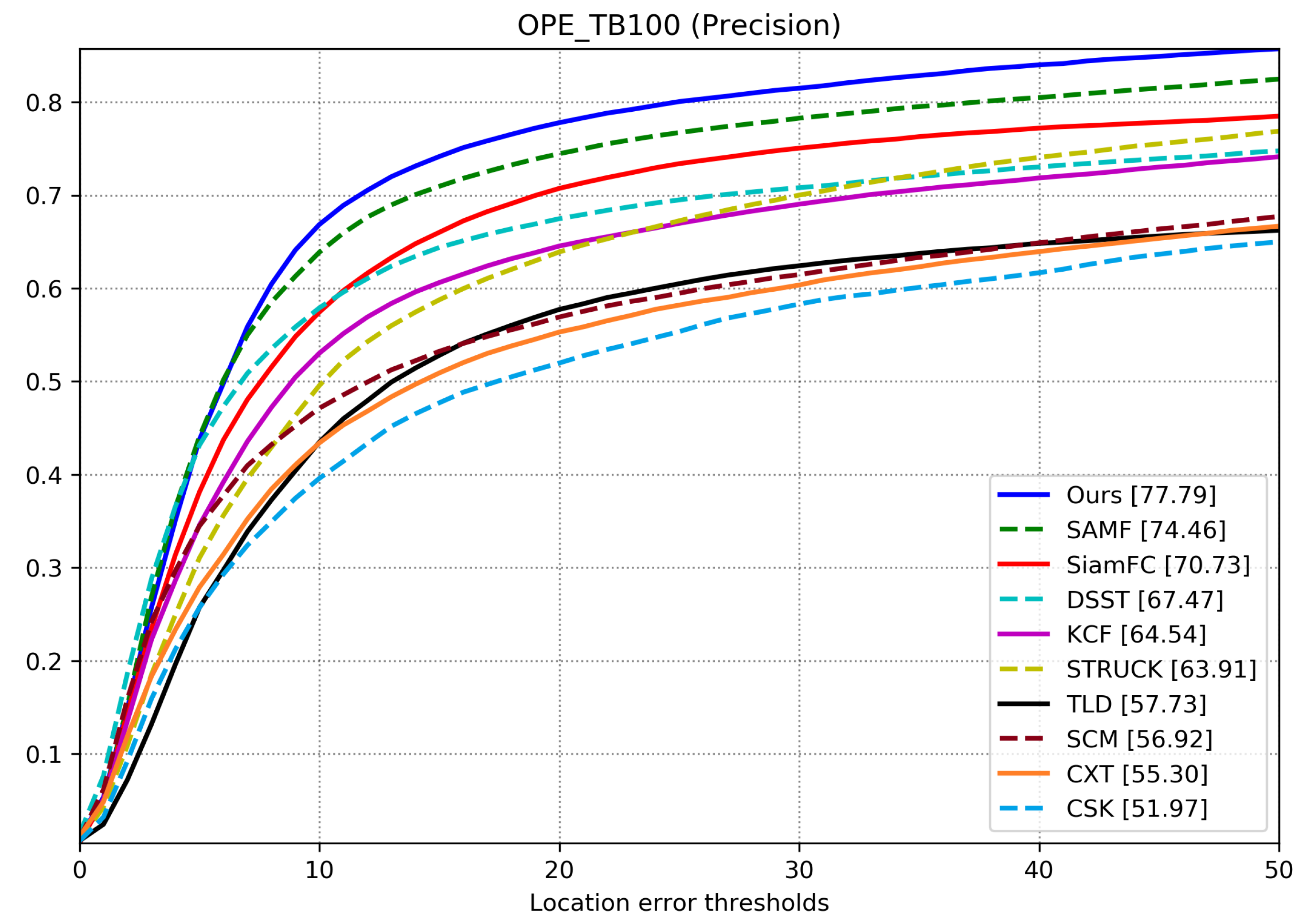
| Methods | Ours | SAMF | SiamFC | DSST | KCF | STRUCK | TLD | SCM | CXT | CSK |
|---|---|---|---|---|---|---|---|---|---|---|
| IV | 70.74 | 66.11 | 63.85 | 66.11 | 59.53 | 50.65 | 50.26 | 56.21 | 47.68 | 45.07 |
| SV | 73.31 | 70.97 | 69.39 | 64.34 | 61.74 | 60.06 | 55.17 | 55.47 | 53.33 | 46.33 |
| OCC | 75.16 | 71.25 | 63.19 | 58.80 | 59.32 | 52.45 | 49.94 | 54.24 | 42.89 | 43.08 |
| DEF | 70.37 | 66.29 | 65.41 | 52.02 | 56.73 | 51.33 | 45.18 | 52.46 | 39.15 | 43.62 |
| MB | 69.77 | 65.54 | 70.09 | 57.96 | 57.20 | 59.49 | 52.73 | 31.94 | 56.54 | 38.85 |
| FM | 73.27 | 64.94 | 68.10 | 56.09 | 57.25 | 62.06 | 53.53 | 35.75 | 54.91 | 42.01 |
| IPR | 70.22 | 70.83 | 67.59 | 67.62 | 62.67 | 64.05 | 58.87 | 53.43 | 60.98 | 53.14 |
| OPR | 75.20 | 73.84 | 68.89 | 64.10 | 63.17 | 60.60 | 55.65 | 57.44 | 52.76 | 49.94 |
| OV | 65.70 | 62.75 | 54.63 | 48.06 | 52.82 | 50.31 | 47.55 | 43.55 | 41.64 | 31.52 |
| BC | 75.19 | 67.66 | 57.93 | 69.09 | 58.61 | 55.01 | 43.24 | 55.00 | 43.78 | 57.42 |
| LR | 66.77 | 70.99 | 61.85 | 54.96 | 55.37 | 62.82 | 53.66 | 55.75 | 49.24 | 36.72 |
| Methods | Ours | SAMF | SiamFC | DSST | KCF | STRUCK | TLD | SCM | CXT | CSK |
|---|---|---|---|---|---|---|---|---|---|---|
| IV | 52.07 | 49.37 | 47.13 | 49.37 | 37.85 | 39.56 | 36.07 | 45.43 | 35.53 | 34.20 |
| SV | 52.63 | 50.15 | 50.97 | 47.46 | 38.50 | 40.75 | 37.21 | 43.28 | 38.76 | 32.84 |
| OCC | 55.37 | 53.60 | 48.18 | 45.56 | 40.81 | 38.56 | 34.48 | 42.08 | 33.02 | 33.36 |
| DEF | 51.75 | 49.50 | 47.79 | 40.62 | 38.94 | 37.66 | 31.90 | 39.09 | 29.71 | 33.06 |
| MB | 52.60 | 52.10 | 54.09 | 47.93 | 40.26 | 46.09 | 40.34 | 31.41 | 40.78 | 32.71 |
| FM | 55.25 | 50.04 | 52.31 | 45.48 | 41.39 | 46.16 | 39.64 | 33.08 | 40.53 | 33.83 |
| IPR | 51.73 | 51.64 | 49.80 | 50.21 | 43.12 | 45.74 | 40.56 | 41.00 | 45.41 | 39.28 |
| OPR | 54.62 | 54.05 | 50.13 | 47.28 | 42.79 | 43.42 | 37.39 | 43.96 | 39.59 | 36.18 |
| OV | 49.19 | 48.03 | 40.16 | 38.59 | 36.85 | 38.42 | 34.23 | 34.81 | 34.38 | 28.31 |
| BC | 53.77 | 51.03 | 42.06 | 50.03 | 40.76 | 42.29 | 31.62 | 43.78 | 34.01 | 41.05 |
| LR | 43.83 | 45.94 | 42.69 | 37.89 | 28.62 | 34.71 | 34.54 | 38.10 | 36.64 | 25.08 |
| Methods | ASB | SI [28] | STS | TR | SV | FM | OCC | OV |
|---|---|---|---|---|---|---|---|---|
| 1 | - | - | - | - | 60.46 | 56.82 | 56.50 | 48.61 |
| 2 | √ | - | - | - | 65.30 | 62.08 | 65.12 | 54.47 |
| 3 | √ | √ | - | - | 66.43 | 63.82 | 65.24 | 56.52 |
| 3 | √ | - | √ | - | 69.03 | 67.10 | 68.83 | 60.46 |
| 4 | √ | - | √ | √ | 73.31 | 73.27 | 75.16 | 65.70 |
| Methods | ASB | SI [28] | STS | TR | SV | FM | OCC | OV |
|---|---|---|---|---|---|---|---|---|
| 1 | - | - | - | - | 38.50 | 41.39 | 40.81 | 36.85 |
| 2 | √ | - | - | - | 46.54 | 47.37 | 47.76 | 41.33 |
| 3 | √ | √ | - | - | 46.78 | 48.12 | 47.43 | 42.03 |
| 3 | √ | - | √ | - | 49.04 | 51.20 | 50.75 | 45.85 |
| 4 | √ | - | √ | √ | 52.63 | 55.25 | 55.37 | 49.19 |
| Methods | DP | AUC | Average Values | ||
|---|---|---|---|---|---|
| 1 | 0.20 | 0.40 | 68.25 | 48.95 | 58.60 |
| 2 | 0.30 | 0.40 | 70.41 | 51.02 | 60.72 |
| 3 | 0.40 | 0.40 | 70.32 | 51.06 | 60.69 |
| 4 | 0.42 | 0.40 | 70.18 | 51.30 | 60.74 |
| 5 | 0.45 | 0.40 | 70.27 | 51.41 | 60.84 |
| 6 | 0.47 | 0.40 | 69.75 | 50.59 | 60.17 |
| 7 | 0.50 | 0.40 | 69.65 | 51.13 | 60.39 |
| Methods | DP | AUC | Average Values | ||
|---|---|---|---|---|---|
| 1 | 0.45 | 0.20 | 67.77 | 49.15 | 58.46 |
| 2 | 0.45 | 0.30 | 70.15 | 51.08 | 60.62 |
| 3 | 0.45 | 0.35 | 68.95 | 50.32 | 59.64 |
| 4 | 0.45 | 0.37 | 69.01 | 50.63 | 59.82 |
| 5 | 0.45 | 0.40 | 70.27 | 51.41 | 60.84 |
| 6 | 0.45 | 0.42 | 70.07 | 50.80 | 60.44 |
| 7 | 0.45 | 0.45 | 67.83 | 50.14 | 58.99 |
| 8 | 0.45 | 0.50 | 69.96 | 51.15 | 60.56 |
| Methods | DP | AUC | Average Values | |
|---|---|---|---|---|
| 1 | 0.20 | 72.07 | 52.52 | 62.30 |
| 2 | 0.22 | 69.27 | 51.82 | 60.55 |
| 3 | 0.25 | 72.91 | 53.15 | 63.03 |
| 4 | 0.27 | 70.96 | 51.93 | 61.45 |
| 5 | 0.30 | 70.70 | 51.05 | 60.88 |
| Methods | ASB | STS | TR | DP | AUC |
|---|---|---|---|---|---|
| 1 | - | - | - | 53.54 | 33.14 |
| 2 | √ | - | - | 55.78 | 39.05 |
| 3 | √ | √ | - | 58.62 | 40.91 |
| 4 | √ | √ | √ | 67.61 | 47.53 |
| Videos | car7 | car9 | group2_1 | person10 | person16 | truck4_2 | wb5 | wb8 |
|---|---|---|---|---|---|---|---|---|
| KCF + ASB + STS | 15.02 | 36.00 | 8.20 | 17.65 | 10.70 | 4.65 | 3.80 | 25.15 |
| Ours | 54.71 | 34.58 | 68.31 | 51.79 | 42.92 | 55.63 | 34.19 | 40.33 |
Disclaimer/Publisher’s Note: The statements, opinions and data contained in all publications are solely those of the individual author(s) and contributor(s) and not of MDPI and/or the editor(s). MDPI and/or the editor(s) disclaim responsibility for any injury to people or property resulting from any ideas, methods, instructions or products referred to in the content. |
© 2025 by the authors. Licensee MDPI, Basel, Switzerland. This article is an open access article distributed under the terms and conditions of the Creative Commons Attribution (CC BY) license (https://creativecommons.org/licenses/by/4.0/).
Share and Cite
Cao, S.; Wang, T.; Li, T.; Fei, S. UAV Real-Time Target Detection and Tracking Algorithm Based on Improved KCF and YOLOv5s_MSES. Machines 2025, 13, 364. https://doi.org/10.3390/machines13050364
Cao S, Wang T, Li T, Fei S. UAV Real-Time Target Detection and Tracking Algorithm Based on Improved KCF and YOLOv5s_MSES. Machines. 2025; 13(5):364. https://doi.org/10.3390/machines13050364
Chicago/Turabian StyleCao, Shihai, Ting Wang, Tao Li, and Shumin Fei. 2025. "UAV Real-Time Target Detection and Tracking Algorithm Based on Improved KCF and YOLOv5s_MSES" Machines 13, no. 5: 364. https://doi.org/10.3390/machines13050364
APA StyleCao, S., Wang, T., Li, T., & Fei, S. (2025). UAV Real-Time Target Detection and Tracking Algorithm Based on Improved KCF and YOLOv5s_MSES. Machines, 13(5), 364. https://doi.org/10.3390/machines13050364