Abstract
As an X–Y table has input saturation constraints or inadequate trajectory planning, the positioning control performance degrades. To overcome this issue, this study proposes an effective anti-integral windup approach based on basic PID control, and then plans a motion trajectory with an S-curve velocity profile to enhance the overall control performance. Finally, the corresponding experiments are conducted to assure the effectiveness of the control framework. The experimental results demonstrate that the proposed control scheme can greatly improve the system positioning precision compared to that without anti-windup when the X–Y table suffers from actuator saturations. Moreover, the corresponding results clearly showcase the superior tracking responses with errors of ±11.23 mm in the X-axis and ±13.63 mm in the Y-axis using the S-curve velocity profile for tracking errors, and ±13.48 mm in the X-axis and ±19.88 mm in the Y-axis applied to the T-curve velocity profile. It is validated and concluded that the proposed control scheme combined with trajectory planning can effectively mitigate integral windup and enhance the positioning precision with the smoother velocity as well as continuous acceleration profiles without vibration.
1. Introduction
Robotic and servo-control systems are key technologies for advanced industrial applications [1,2]. In order to create an industrial robot capable of undertaking more complex works, the control technologies require high speed and high precision characteristics with a good dynamic performance. Thus, the research issue in [3,4,5] has become increasingly important: controlling industrial robots in a way makes them respond quickly to the predetermined trajectory commands while maintaining a high dynamic tracking accuracy, aiming to achieve stable operation. For most servo-based motion control systems, controllers are designed in a closed loop to control the velocity and position of machines to generate desired motions. The main challenge lies in achieving precise positioning while minimizing vibration and reducing overshoot in both the position and velocity.
Mechanically feasible and smooth paths with optimized time and minimized overshoots are consistently the goals of path planning. Erkorkmaz et al. [6] proposed a method for developing optimized point-to-point motion profiles to achieve fast motion with minimized vibration, commonly referred to as the S-curve model. However, a key limitation is its complexity in implementation, particularly for systems requiring real-time computation, as it demands precise tuning and significant computational resources. Berscheid and Kröger [7] proposed an online trajectory generation (OTG) algorithm that generates time-optimal, jerk-limited trajectories for arbitrary target states. The algorithm is capable of handling complete kinematic states (position, velocity, and acceleration), providing smooth motion and real-time performance across multiple degrees of freedom (DoFs).
Consider that the servo-control systems always operate in a wide range of conditions and different environments, and the control inputs may reach the actuator limits. In addition, the higher accuracy requirements and faster response time needed in the servo-control system mean that even small changes on the control commands may have a great impact on the operation system. It turns out that the feedback loop does not perform effectively, and the closed-loop system becomes an open-loop system as actuators remain at its limits, regardless of the system outputs. One of main reasons is that the controller’s integral component is improperly designed. Error signals still continue accumulation while control inputs meet saturation. This causes the integral term to grow excessively large. The phenomenon is known as integral windup or simply windup. Regarding this issue, there have been numerous studies conducted to address the phenomenon of windup. Shin et al. [8] surveyed a new anti-windup technique for the PI structure which is based on the back-calculation method. The proposed novel technique eliminated the problem caused by the fixed-back calculation gain in the traditional anti-windup scheme and prevented a large overshoot or untimely saturation withdrawing in the Permanent Magnet Synchronous Motor (PMSM) servo system. In [9], Ohishi et al. presented a comprehensive investigation into anti-windup strategies, addressing the undesired windup phenomenon through specifically designed current and speed controllers for field-oriented control of PMSM systems. Their approach demonstrates significant advantages in stability enhancement and an improved dynamic performance under operating conditions. Yet, their work could be further enhanced to address situations of systems that exhibit large overshoots or oscillatory responses when handling quick, large speed references with large load torques. Besides, the dynamic anti-windup compensators for time-varying or nonlinear systems have also been thoroughly discussed by means of solvability LMIs and neural networks [10,11,12]. According to the aforementioned literature, we realize the integral action in servo-control systems may produce unexpected change if an actuator input becomes saturated or if the process input unexpectedly changes.
These control challenges reflect the limitations on servo-control implementations, particularly in applications demanding high precision and high-speed operation. The integral windup issues present in traditional control methods interact with acceleration discontinuities in trajectory planning, which constrain performance robustness. Hence, the proposed research is conducted to meet this technical requirement through the improvement of trajectory smoothness and the control system saturation problem. By integrating S-curve velocity profiles with anti-windup PID control strategies, a comprehensive solution can be established to ensure smooth and continuous motion trajectories while effectively handling controller saturation issues.
In this study, we present a motion trajectory planning, i.e., S-curve velocity profile, for an X–Y table to improve the issue of acceleration discontinuity in the T-curve velocity profile [13]. Additionally, an anti-windup-based PID control strategy is integrated to mitigate the negative effects of actuator saturation, thereby enhancing control precision and performance. The main contributions are as follows: (1) we propose a double S-curve velocity profile theory for X–Y tables, designed with seven segments of constant jerk to achieve a smoother motion trajectory without vibration. By reducing stress and vibration effects in the transmission system, it enhances motion stability compared to trapezoidal velocity profiles, making it suitable for high-precision motion control. (2) To achieve rapid and precise trajectory tracking, the anti-windup algorithm-based positioning controller is proposed to complete rapid and precise trajectory tracking. (3) Practical experiments are conducted on a physical X–Y table utilizing high-resolution sensors and servo motors. In this process realization, the anti-windup-based PID positioning controller and trajectory planning in real-world scenarios is integrated into the hardware implementation. The results show that the effectiveness and feasibility of the proposed method have been assured through experimental verification, exhibiting the expected performance of S-curve velocity planning.
2. The Design of Double S-Curve Velocity Profile
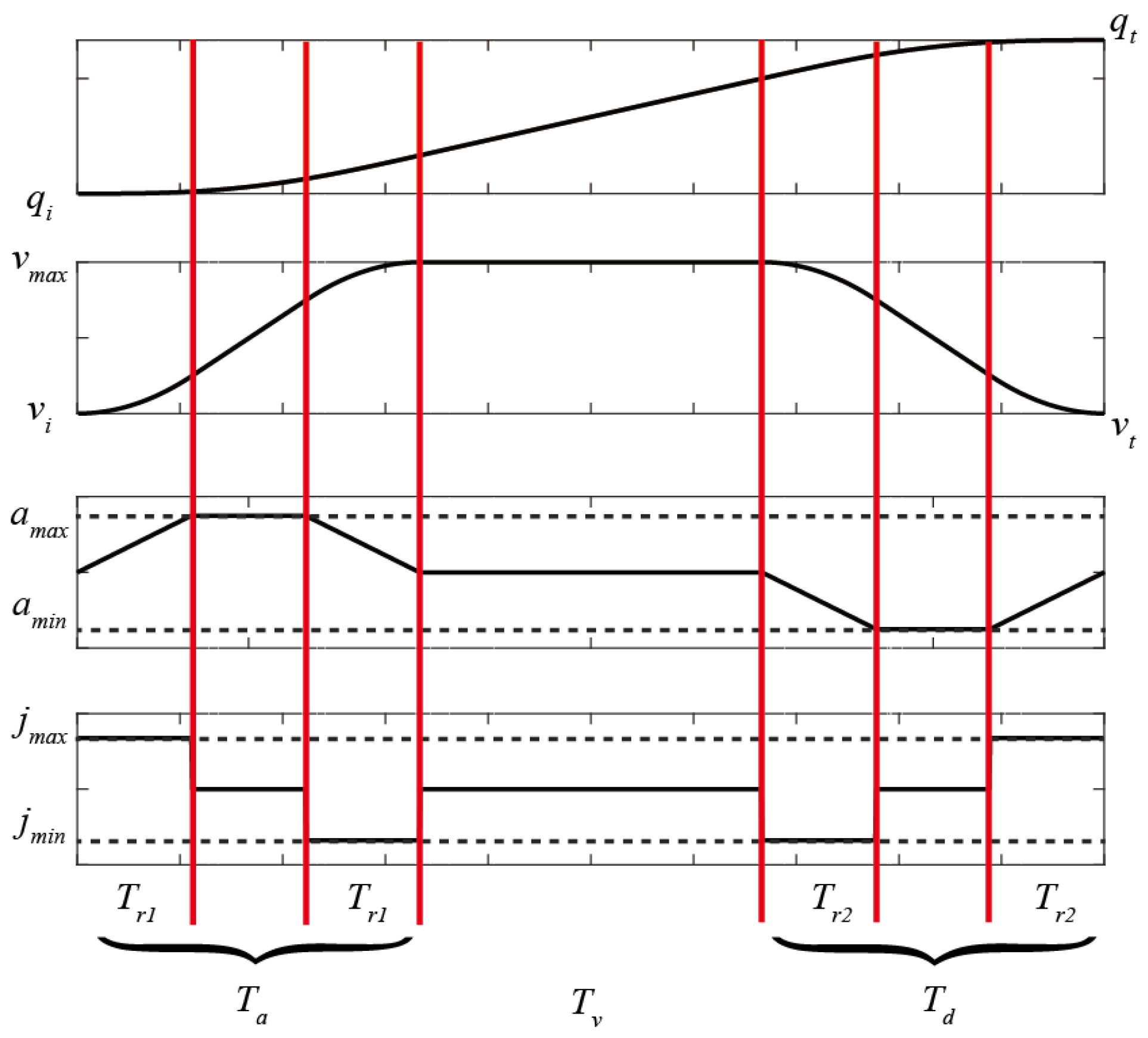
A common, widely-used trapezoidal velocity (i.e., T-curve) motion profile presents a discontinuous acceleration [14,15,16]. To reduce the change rate of the acceleration (jerk), we first constructed a symmetrical T-curve acceleration/deceleration (Acc/Dec) motion trajectory with confined jerk, acceleration, and velocity point-to-point (PTP) motion applications. A schematic diagram of the jerk, acceleration, velocity, and displacement profiles is shown in Figure 1. Generally, the design of the S-curve velocity trajectory involves the following parameters: , , , , , , , which represent the initial position, final position, initial velocity, final velocity, maximum/minimum velocities, and maximum/minimum accelerations, respectively.
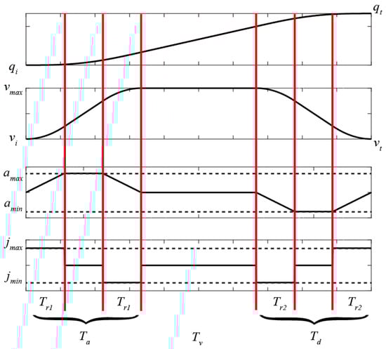
Figure 1.
Profiles of the position, velocity, acceleration, and jerk for the double S-curve velocity trajectory.
The double S-curve velocity profile is divided into seven segments with the following time intervals:
The time spent to transition from the jerk phase to the constant acceleration phase .
The time spent to transition from the deceleration jerk phase to the constant negative acceleration phase.
The period of the constant acceleration phase.
The period of the constant velocity phase.
The period of the constant negative velocity phase.
Assuming symmetric constraints where maximum and minimum values are equal in magnitude but opposite in sign (i.e., , , ), the displacement , velocity , acceleration , and jerk during each time interval, starting from to can be expressed as follows:
Acceleration section:
Constant velocity section:
Deceleration section:
3. Positioning Controller with an Anti-Windup Algorithm Design
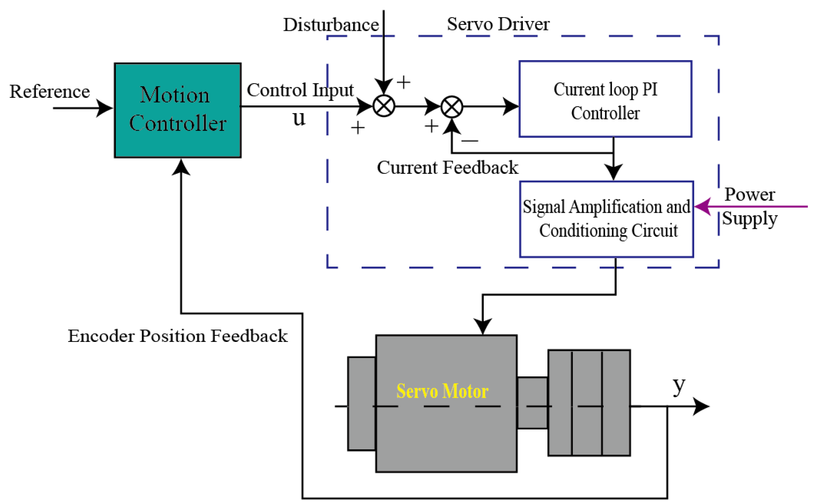
In order to develop a positioning controller with sufficient adaptability to handle various velocity planning strategies (e.g., T-curve or S-curve) in the servo -control system [17,18,19,20] shown in Figure 2, an anti-windup algorithm based on the PID controller is introduced within the motion controller block.

Figure 2.
Illustration of a typical servo-motor-control system.
The basic PID positioning controller [17] can be represented as follows:
where represents a proportional gain; signifies the integral gain; is the derivative gain, and denotes the filter parameter of the derivative term. Its discretized form can be obtained in Equation (9) from its equivalent continuous-time counterpart Equation (8), given by the following:
where denotes the sampling period. Based on Equation (9), the control input in discrete time can be derived as follows:
where , , and are the proportional, integral, and derivation control terms, respectively. These three terms can be represented as:
where As the control input is an input voltage limited by a devise saturation, and the relationship can be expressed as:
where represents a limit value of the control input, is a signum function which determines the sign of the control input, and denotes the computed control input. The saturation probably occurs due to the basic PID controller with the integral action. Therefore, an anti-windup control scheme, namely the back-calculation algorithm, is introduced to address the integral windup problem.
Back-calculation algorithm design:
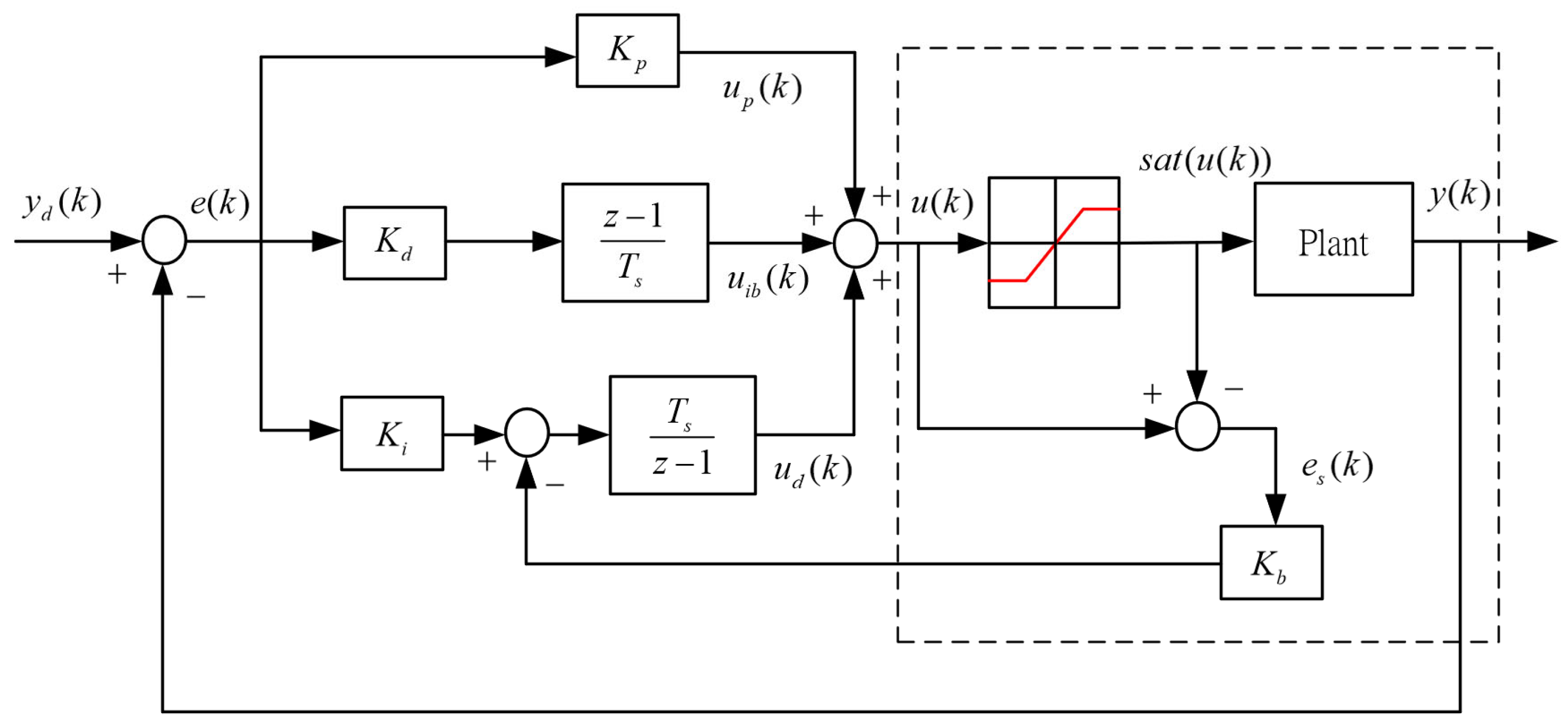
The characteristic of this back-calculation algorithm is that a gain based on the feedback loop is designed to reduce the effect of the integral windup. The overall control block diagram of the anti-windup based PID controller is shown in Figure 3.
where denotes the back-calculation integral control term, is a back-calculation gain, and . In this way, the integral control term in Equation (10) is substituted with in Equation (15). Hence, the new control input based on the back-calculation-algorithm is yielded as:
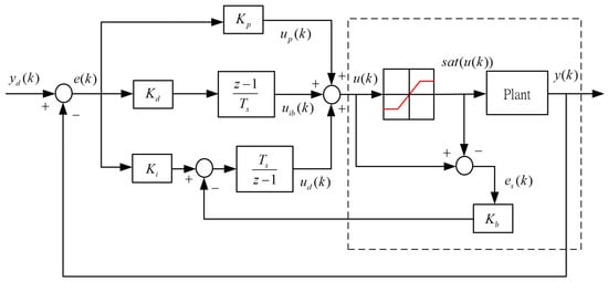
Figure 3.
Block diagram of the back-calculation-based PID controller [13].
Then, the next section presents the experimental validation and complete result discussions of the proposed control scheme. These experiments are specifically planned to evaluate how the double S-curve velocity profile works in conjunction with the anti-windup algorithm under real-world conditions. The experimental setup, parameter selections, and testing procedures are carefully configured to examine both the individual and combined effects of the proposed techniques on positioning accuracy, overshoot reduction, and overall system performance.
4. Experimental Validation and Result Discussion
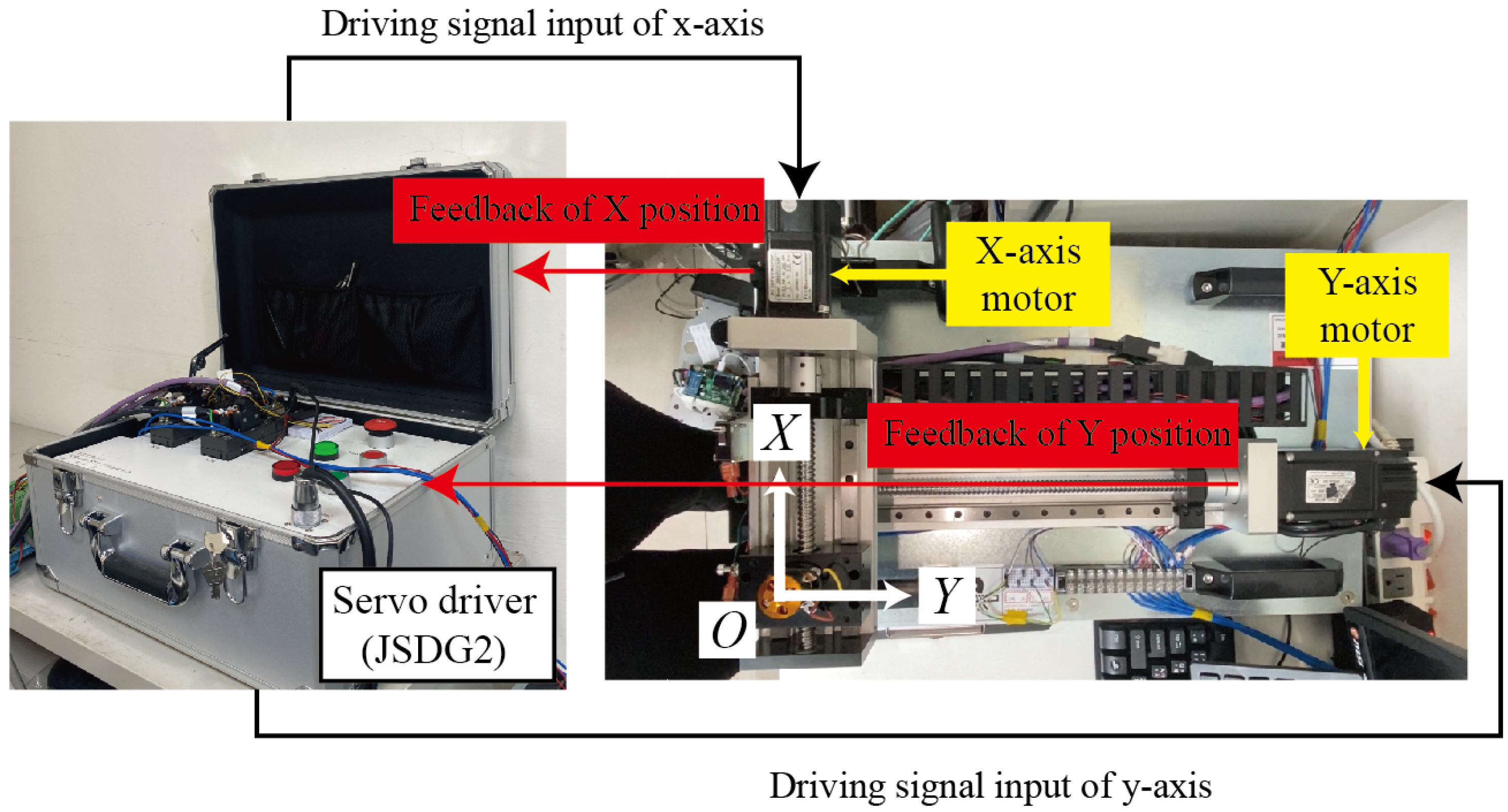
A servo-based X–Y table can perform planar motion and is utilized to experimentally validate the effectiveness of the proposed back-calculation-based PID control combined with the S-curve velocity trajectory. The experimental setup of the X–Y table is shown in Figure 4. In this configuration, two servo motors (JSMA-PUC01) and (TSX06401C-3N33) along with the servo drivers (JSDG2) manufactured by TECO Inc., Taipei, Taiwan consist of the X–Y table. In addition, the 17-bits incremental rotation encoders are included in the servo motors that can measure a positioning resolution of up to 0.4 mm, and communication with each component is established through the PCIe protocol.
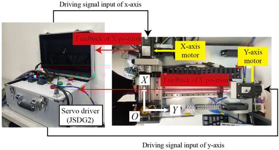
Figure 4.
The experimental X–Y table based on the servo-motor system.
The servo system receives motion controller commands (e.g., voltage) and tracks the specified motion trajectory. In the experiment, the control parameters are shown in Table 1. The PID controller gains are determined empirically through a series of experiments. By observing the system response to various gain settings, the parameters are adjusted step by step to achieve the desired performance in terms of stability, responsiveness, and minimal overshoot. To compare the performance differences between the traditional control methods (i.e., PID control) and the anti-windup-based PID control under saturation conditions, specific reference trajectories (i.e., S-curve velocity profile) are designed. In terms of motion control applications, trajectory planning is crucial for the assessment of the system performance. The experimental results demonstrate that the implemented anti-windup algorithm is effective in nonlinear regions. Specifically, these algorithms reliably maintain system stability and demonstrably improve the control performance, particularly under input saturation conditions. Although other uncertainties are present, they can be tackled by the basic PID controller. Here, the quadrilateral trajectory is designed and followed by the implementation utilizing the S-curve velocity profile.

Table 1.
The control parameters used in the experiment.
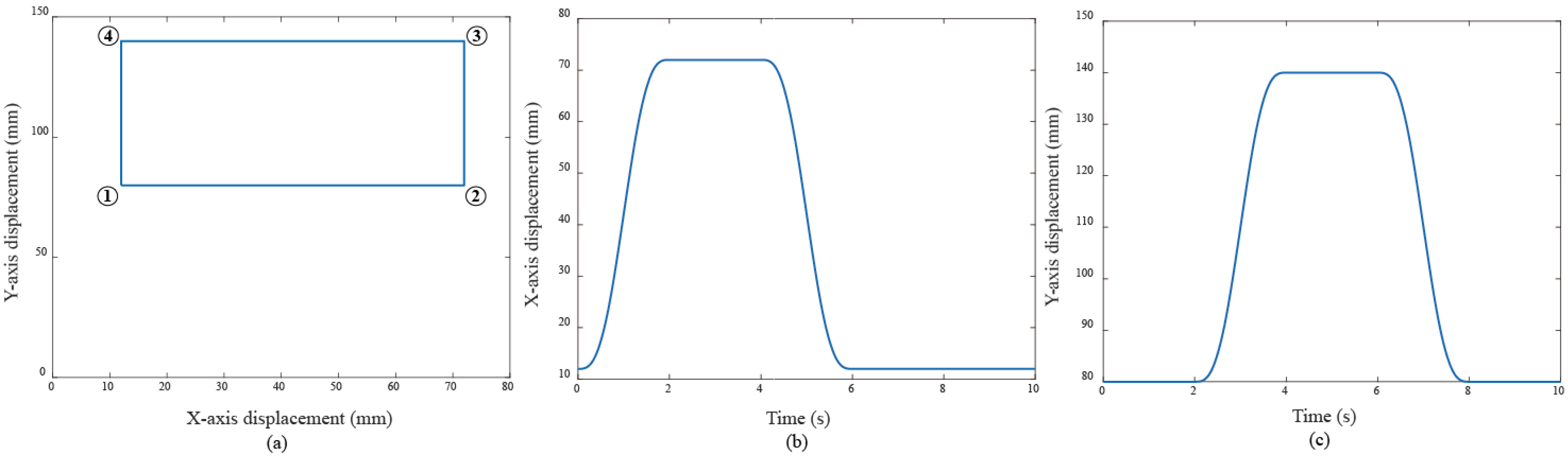
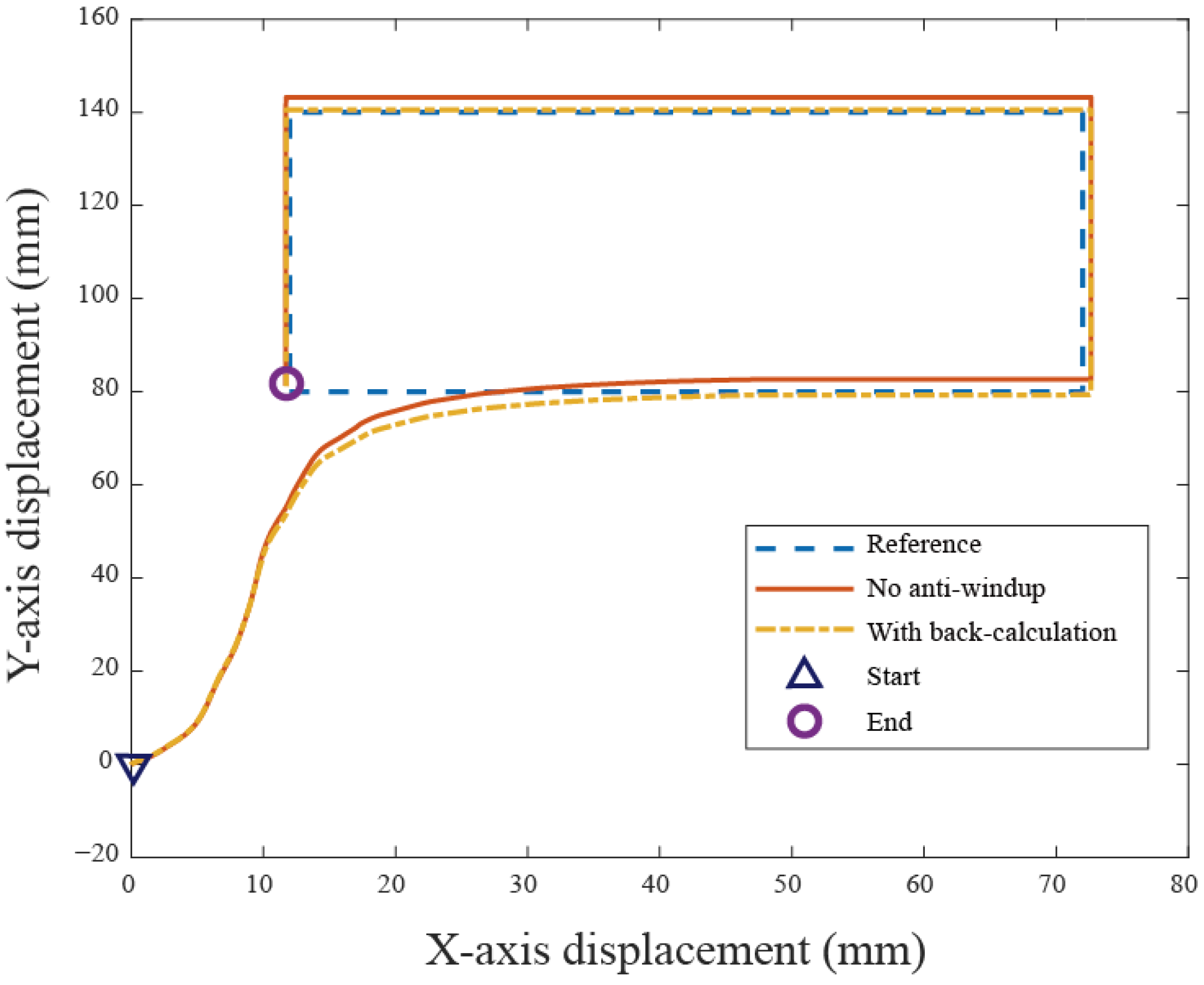
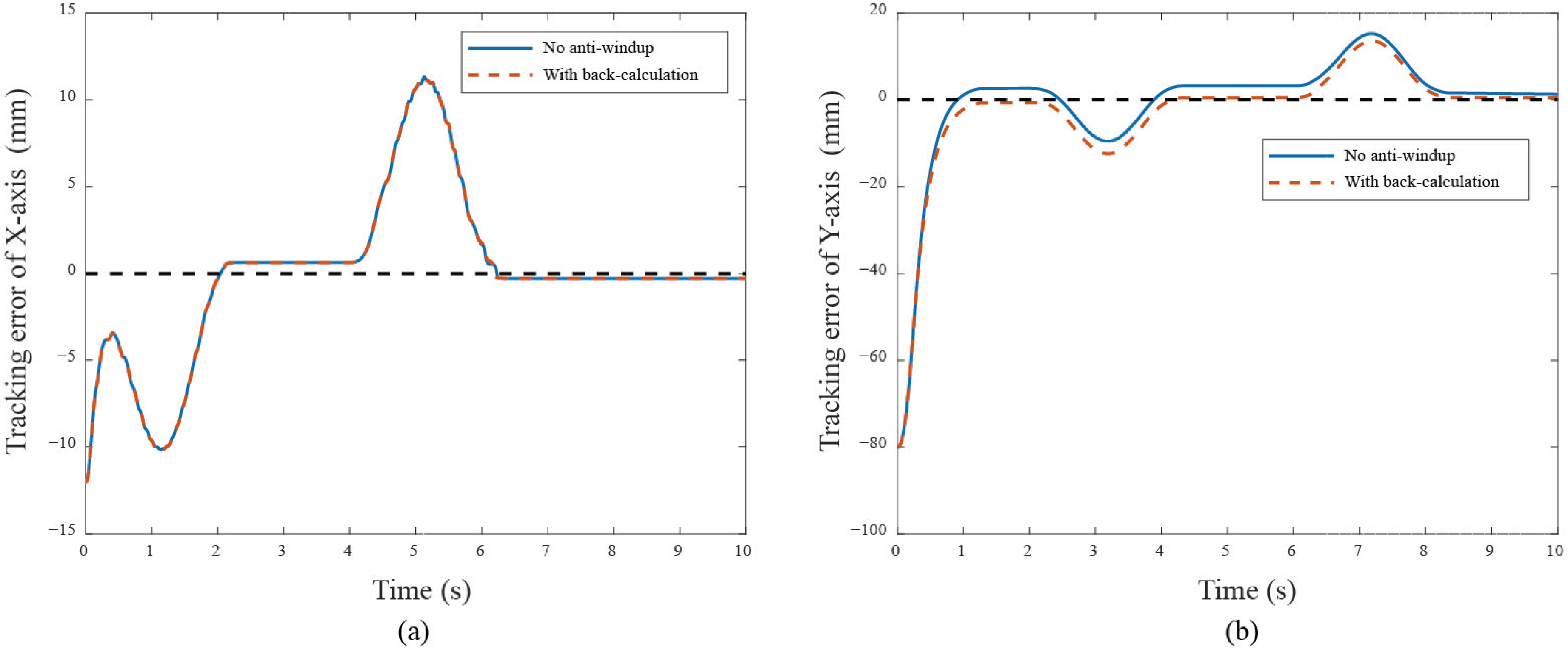
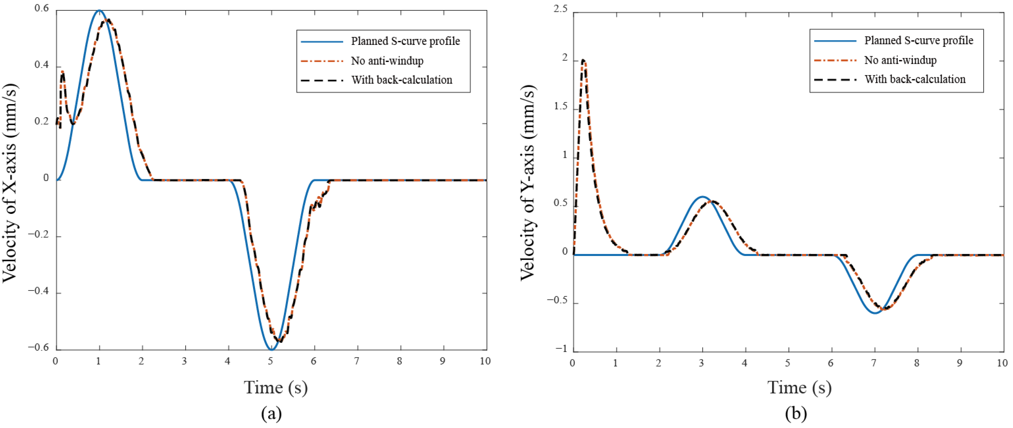
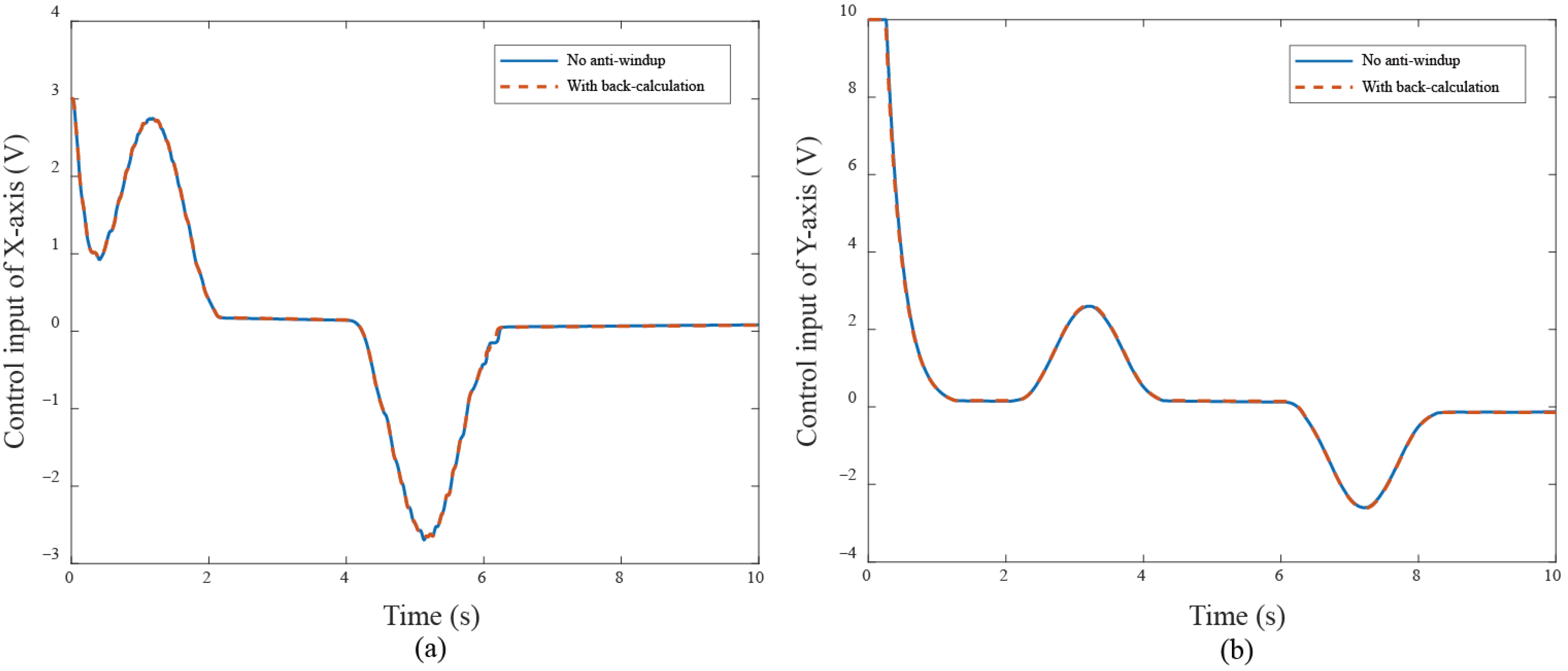
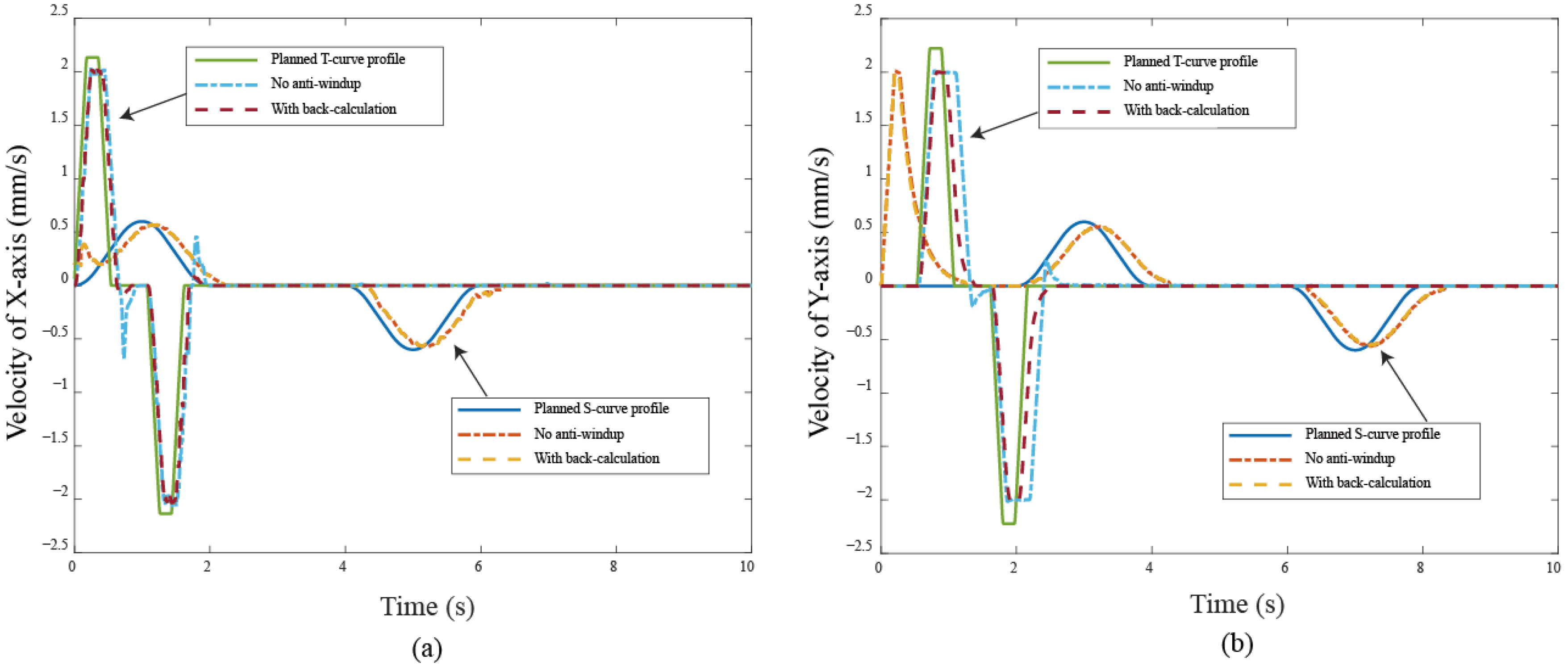
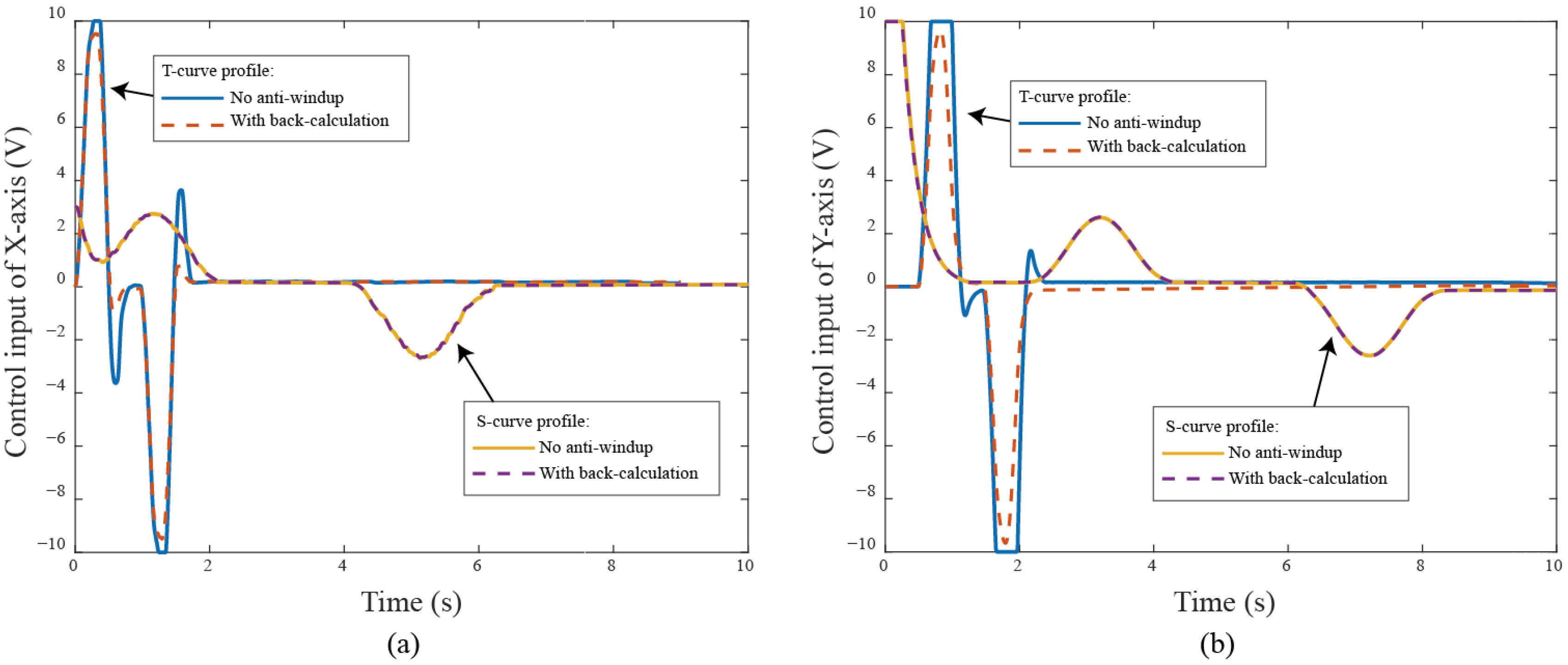
The quadrilateral trajectory is designed with a side length of 60 mm × 60 mm based on the S-curve velocity profile, and the coordinates of four corner points ①, ②, ③, ④ in turn are (12, 80), (72, 80), (72, 140) and (12, 140), respectively, as illustrated in Figure 5. Inherently, it possesses smoother acceleration characteristics compared to the trajectory with the T-curve velocity profile, resulting in a significantly smoother execution process. In this configuration, the maximum jerk is set to be mm/s3 for both motors. Furthermore, maximum acceleration and maximum velocity are identical for both motors and set to 0.009 mm/s2 and 0.6 mm/s, respectively. In the experiment, the X–Y table system starts from the initial point (0, 0). The configuration facilitates the observation of the system’s transient response, followed by an analysis of the individual velocity responses. In the case of the quadrilateral trajectory with S-curve velocity profile, the y-axis response is the primary focus in the system, as the x-axis response is immaterial due to the lack of the saturation. Figure 6 showcases the trajectory-tracking responses of the quadrilateral trajectory employing an S-curve velocity profile. This clearly displays the occurrence of the windup phenomenon, and the proposed anti-windup algorithm can substantially improve the overshoot and obtain superior performance compared with the one without the anti-windup scheme. The snapshots at the specific time in the experimental process are recorded and shown in Figure 7. These results demonstrate that the anti-windup algorithm achieves varying degrees of effectiveness in the experiment. Figure 8 shows the tracking error responses comparing the accuracy range with and without the anti-windup algorithm. The maximum steady-state error is ±14.32 mm without anti-windup, and ±13.63 mm in the back-calculation algorithm for the quadrilateral path with an S-curve velocity profile. The corresponding velocity responses of each axis are shown in Figure 9 for the X and Y axes. It is well known that a servo-control system’s ability to follow a specific path, based on the previously designed S-curve velocity profiles, is affected by the absence of anti-windup algorithms, resulting in a more significant dynamic error. Conversely, the implementation of the proposed control algorithms enables the velocity response to achieve a closer approximation to the planned velocity along the quadrilateral path. Furthermore, experimental evidence indicates that while S-curve velocity profiles inherently exhibit a transient response, they demonstrably yield a smoother velocity response when contrasted with the T-curve profile. Figure 10 display their corresponding control inputs in different designed motion paths. Furthermore, compared with our earlier study in [13], the S-curve velocity profile yields a smoother velocity transition than the one using the trapezoidal T-curve velocity profile, as illustrated in Figure 11, resulting in enhanced motion stability and positioning precision. Figure 12 shows the control input responses in comparison with Ref. [13]. It can be observed that the S-curve also produces a smoother control input response compared with that using the T-curve velocity profile, whereas the T-curve produces larger oscillations both without anti-windup and with the back-calculation algorithm. Overall, it is evident that without the anti-windup algorithm, the servo-control system suffers varying degrees of saturation issues, leading to a significant increase in both overshoot and tracking errors during the saturation period. The corresponding control performance indices are presented in Table 2. In summary, the back-calculation method based on the PID controller demonstrates the highest level of stability and the smallest tracking error, while the designed S-curve velocity profile minimizes jerk to regulate the system’s dynamic response.
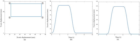
Figure 5.
(a) The quadrilateral curve designed using the S-curve velocity profile in the experiment; (b,c) are the independent motion commands for both servo motors, respectively.

Figure 6.
Experimental results comparing to the case without the anti-windup and with the back-calculation algorithm for the quadrilateral curve obtained using the S-curve velocity profile.

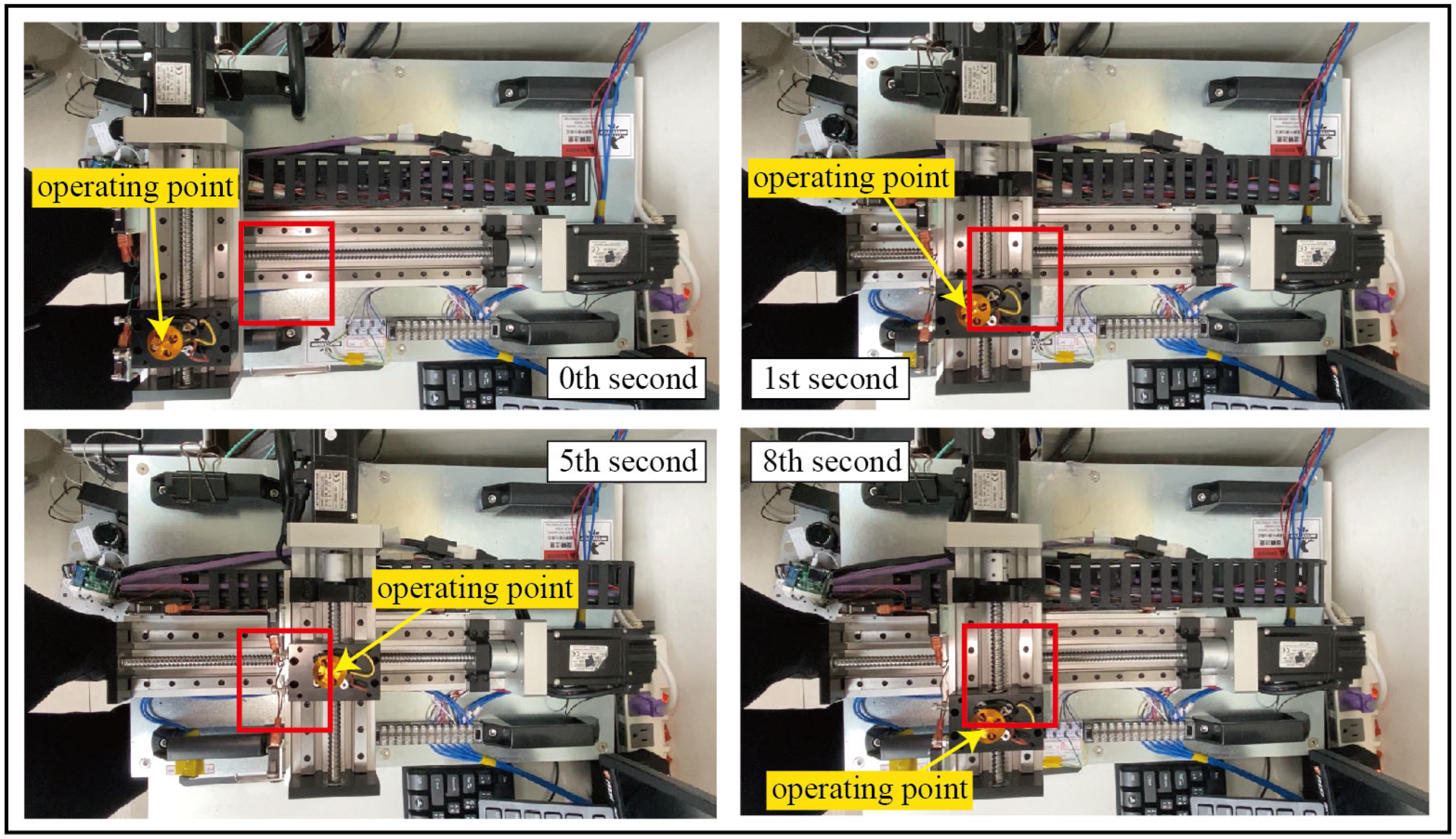
Figure 7.
Snapshots of an experimental process using the back-calculation while executing the quadrilateral path.
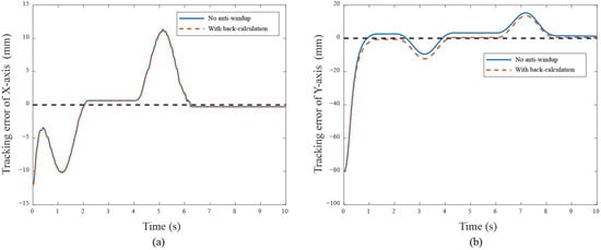
Figure 8.
The tracking error responses for the (a) X-axis and (b) Y-axis for the quadrilateral curve.
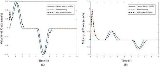
Figure 9.
The corresponding velocity responses for the (a) X-axis and (b) Y-axis for the quadrilateral curve.
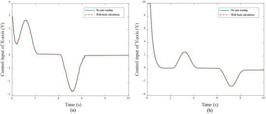
Figure 10.
The corresponding control input responses for the (a) X-axis and (b) Y-axis for the quadrilateral curve.
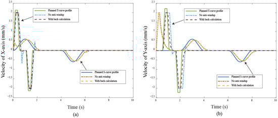
Figure 11.
Comparison of the velocity responses in Ref. [13] for the (a) X-axis and (b) Y-axis.
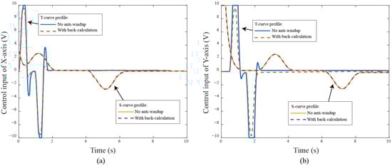
Figure 12.
Comparison of the control input responses in Ref. [13] for the (a) X-axis and (b) Y-axis.
Table 2.
The overshoot comparisons under different motion trajectories and with or without anti-windup for the X–Y table.
5. Conclusions
This study proposes and evaluates the anti-windup algorithm (i.e., back-calculation algorithm) based on the PID controller for the servo-based X–Y table. The experimental results indicate that the back-calculation algorithm attains a superior control performance by preventing severe tracking errors caused by integral windup to that without using anti-windup. The tracking results demonstrate that the back-calculation algorithm achieves the most precise positioning control, with errors of ±13.48 mm in X-axis and ±19.88 mm in Y-axis using T-curve velocity planning, and errors of ±11.23 mm in the X-axis and ±13.63 mm in the Y-axis using S-curve velocity planning for the quadrilateral path. It is concluded that back-calculation-algorithm-based PID control exhibits a significantly improved positioning control performance, including reduced overshoot and shorter settling time, effectively mitigating the control input saturation effects. Additionally, the planned motion trajectory based on the S-curve velocity profile indeed achieves continuous acceleration without vibration and further enhances the positioning precision.
Author Contributions
Conceptualization, H.-M.W. and C.-W.C.; methodology, H.-M.W., C.-W.C. and C.-Y.N.; validation, H.-M.W. and C.-Y.N.; writing—original draft preparation, H.-M.W.; writing—review and editing, H.-M.W. and C.-W.C.; supervision and funding acquisition, H.-M.W. All authors have read and agreed to the published version of the manuscript.
Funding
This research received no external funding.
Data Availability Statement
Data are contained within this article.
Conflicts of Interest
The authors declare no conflicts of interest.
References
- Kilikevicius, S.; Baksys, B. Analysis of insertion process for robotic assembly. J. Vibroeng. 2007, 9, 35–40. [Google Scholar]
- Zheng, H.; Wu, M.; Shen, X. Pneumatic variable series elastic actuator. J. Dyn. Syst. Meas. Control 2016, 138, 081011. [Google Scholar] [CrossRef] [PubMed]
- Wang, Y.; Xu, Q. Design and Fabrication of a New Dual-Arm Soft Robotic Manipulator. Actuators 2019, 8, 5. [Google Scholar] [CrossRef]
- Yao, J.; Jiao, Z.; Ma, D. Adaptive Robust Control of DC Motors with Extended State Observer. IEEE Trans. Ind. Electron. 2013, 61, 3630–3637. [Google Scholar] [CrossRef]
- Wu, Y.; Wang, H. Application of Fuzzy Self-tuning PID Controller in Soccer Robot. In Proceedings of the 2008 IEEE International Symposium on Knowledge Acquisition and Modeling Workshop, Wuhan, China, 21–22 December 2008; pp. 14–17. [Google Scholar]
- Erkorkmaz, K.; Altintas, Y. High-speed CNC system design. Part I: Jerk-limited trajectory generation and quintic spline interpolation. Int. J. Mach. Tools Manuf. 2001, 41, 1323–1345. [Google Scholar]
- Berscheid, L.; Kröger, T. Jerk-limited real-time trajectory generation with arbitrary target states. arXiv 2021, arXiv:2105.04830. [Google Scholar]
- Shin, H.-B.; Park, J.-G. Anti-Windup PID Controller With Integral State Predictor for Variable-Speed Motor Drives. IEEE Trans. Ind. Electron. 2012, 59, 1509–1516. [Google Scholar] [CrossRef]
- Ohishi, K.; Hayasaka, E.; Nagano, T.; Harakawa, M.; Kanmachi, T. High-Performance Speed Servo System Considering Voltage Saturation of a Vector-Controlled Induction Motor. IEEE Trans. Ind. Electron. 2006, 53, 795–802. [Google Scholar] [CrossRef]
- Yang, F.; Li, J.; Dong, H.; Shen, Y. Proportional–Integral-Type Estimator Design for Delayed Recurrent Neural Networks Under Encoding–Decoding Mechanism. Int. J. Syst. Sci. 2022, 53, 2729–2741. [Google Scholar] [CrossRef]
- Luo, B.; Liu, D.; Huang, T.; Yang, X.; Ma, H. Multi-Step Heuristic Dynamic Programming for Optimal Control of Nonlinear Discrete-Time Systems. Inf. Sci. 2017, 411, 66–83. [Google Scholar] [CrossRef]
- Alanis, A.Y.; Alvarez, J.G.; Sanchez, O.D.; Hernandez, H.M.; Valdivia-G, A. Fault-Tolerant Closed-Loop Controller Using Online Fault Detection by Neural Networks. Machines 2024, 12, 844. [Google Scholar] [CrossRef]
- Chen, C.; Wu, H.; Nian, C. A Class of Anti-Windup Controllers for Precise Positioning of an X-Y Platform with Input Saturations. Electronics 2025, 14, 539. [Google Scholar] [CrossRef]
- Heo, H.J.; Son, Y.; Kim, J.M. A Trapezoidal Velocity Profile Generator for Position Control Using a Feedback Strategy. Energies 2019, 12, 1222. [Google Scholar] [CrossRef]
- Ha, C.W.; Lee, D. Analysis of Embedded Prefilters in Motion Profiles. IEEE Trans. Ind. Electron. 2017, 65, 1481–1489. [Google Scholar] [CrossRef]
- Bai, Y.; Chen, X.; Sun, H.; Yang, Z. Time-Optimal Freeform S-Curve Profile Under Positioning Error and Robustness Constraints. IEEE/ASME Trans. Mechatron. 2018, 23, 1993–2003. [Google Scholar] [CrossRef]
- Roman, R.-C.; Radac, M.-B.; Precup, R.-E.; Petriu, E.M. Virtual Reference Feedback Tuning of Model-Free Control Algorithms for Servo Systems. Machines 2017, 5, 25. [Google Scholar] [CrossRef]
- Pahk, H.J.; Lee, D.S.; Park, J.H. Ultra precision positioning system for servo motor–piezo actuator using the dual servo loop and digital filter implementation. Int. J. Mach. Tools Manuf. 2001, 41, 51–63. [Google Scholar] [CrossRef]
- Ramírez, A. Modeling and tracking control of a pneumatic servo positioning system. In Proceedings of the 2013 II International Congress of Engineering Mechatronics and Automation (CIIMA), Bogota, Colombia, 23–25 October 2013; pp. 1–6. [Google Scholar]
- Alwal, L.A.; Kihato, P.K.; Kamau, S.I. DC servomotor-based antenna positioning control system design using PID and LQR controller. In Proceedings of the 2016 Sustainable Research and Innovation (SRI) Conference, Nairobi, Kenya, 4–6 May 2016; pp. 30–35. [Google Scholar]
Disclaimer/Publisher’s Note: The statements, opinions and data contained in all publications are solely those of the individual author(s) and contributor(s) and not of MDPI and/or the editor(s). MDPI and/or the editor(s) disclaim responsibility for any injury to people or property resulting from any ideas, methods, instructions or products referred to in the content. |
© 2025 by the authors. Licensee MDPI, Basel, Switzerland. This article is an open access article distributed under the terms and conditions of the Creative Commons Attribution (CC BY) license (https://creativecommons.org/licenses/by/4.0/).