Design of Rotors in Centrifugal Pumps Using the Topology Optimization Method and Parallel Computing in the Cloud ^†

Abstract

Designing flow machines is challenging due to numerous free geometrical parameters. This work aims to develop a parallelized computational algorithm in MATLAB version R2020a to design the rotor of a radial flow in a centrifugal pump using the finite-element method (FEM), topology optimization method (TOM), and parallel cloud computing (bare-metal vs. virtual machine). The goal is to minimize a bi-objective function comprising energy dissipation and vorticity within half a rotor circumference. When only minimizing energy dissipation (wd = 1, wr = 0), the performance achieved is 5.88 Watts. Considering both energy dissipation and vorticity (wd = 0.8, wr = 0.2), the performance is 5.94 Watts. These topology results are then extended to a full 3D model using Ansys Fluent version 18.2 to validate the objective functions minimized by TOM. The algorithm is parallelized and executed on multiple CPU cores in the cloud on two different platforms: Amazon Web Services (virtual machine) and Equinix (bare-metal machine), to accelerate the blade design process. In conclusion, mathematical optimization tools aid engineering designers in achieving non-intuitive designs and enhancing results.

1. Introduction

Turbomachines are widely distributed in the industry and are used in various applications at different scales. They can be not only large-sized machines, such as the turbines used in thermoelectric and hydroelectric plants, but also small-sized pumps used in medical applications, such as auxiliary blood pumps [1]. However, the design and performance prediction of these machines remain a difficult task, mainly due to the large number of geometric parameters involved. In addition, the cost and significant time of trial-and-error methods to build prototypes reduce manufacturers’ profit margins. Numerical simulations can provide very precise information on the behavior of fluid flow in these machines, thus helping engineers to obtain a comprehensive evaluation of the performance of a particular design [2,3]. But, it is important to mention that this kind of solution must be combined with accelerated methods such as parallel programming to improve the time consumption of the calculation of fluid flow problems. Under this context, this article deals with parallel computing in the cloud, using the topology optimization method as a solution to the minimization of an objective’s functions.

In the literature, there are few works related to centrifugal pumps using accelerated methods. For example, Liang Dong et al. [4] studied and verified a large-scale parallel mesh generation algorithm applied to a centrifugal pump. They used the Sutherland–Hodgman (S-H) algorithm for cropping and segmenting grid point sets on the surface mesh of a centrifugal pump that was tested using the Tianhe-2 supercomputer. The results show that the algorithm can generate 3D unstructured grid elements in 5 min, and the parallel efficiency can achieve 80%. In addition, Alessandro et al. [5] studied the fluid flow inside a centrifugal pump in high-performance numerical simulations using GPU cards. The simulations in this work were carried out at the best-efficiency point (BEP) for single-phase flow with four different turbulence models. The comparison at the BEP showed that the integral quantity-based results were not sensitive to the turbulence model.

Some other works found in the literature are related to the optimization of these centrifugal flow machines [6,7,8,9]. Shahram Derakhshan [6] employed a global optimization method based on artificial neural networks (ANN) and the artificial bee colony (ABC) algorithm. Derakhshan solved the Navier–Stokes equations to redesign the geometry of an impeller and improve the performance of a Berkeh brand pump 32–160. Moreover, Wen Guan Li [7] used the singularity method to develop an inverse problem in order to design optimized impeller blades for centrifugal pumps. This work estimated the hydraulic performance using a computational fluid dynamics (CFD) code and obtained an improvement of more than 5% in its efficiency. Furthermore, Lei et al. [8] used the direct and inverse iterative method to design an optimized pump impeller compared to the traditional design method. In addition, Gölcü et al. [9] optimized the efficiency of a centrifugal pump by inserting splitters between the blades. The results showed that the splitter between the blades causes a negative effect on the performance of the pump impeller with six and seven blades, but when the splitter blade was added to the impeller with five blades, the efficiency was increased. This research shows that the impeller of a centrifugal pump has an important influence on the performance of these rotatory machines. In addition to these studies, there are other various works [10,11,12,13] that highlight that the study of fluid flow in centrifugal pumps is a broad research area that must be approached in three significantly ways: (a) by computational algorithms, (b) by commercial software that solves the Navier–Stokes equations, and (c) by experimental prototypes. Zhao et al. [10] studied the optimization variables and control impeller for the optimization design. They concluded that the impeller reaches maximum efficiency when the linear segment angle is −2.886°. Wang et al. [11] carried out an optimization process for impellers based on numerical simulation, Latin hypercube sampling (LHS), the surrogate model, and the genetic algorithm (GA) in order to improve the efficiency of residual heat-removal pump. They concluded that the optimization increased efficiency by 8.34% under the design point.

Regarding computational algorithms, topology optimization is seen as an alternative method for the optimal design of centrifugal machines [14,15].

Topology optimization is a mathematical method that spatially optimizes the distribution of material within a defined domain. This optimization method distributes a fluid or solid in the design domain, minimizing or maximizing a predefined objective function. A conventional method for solving an objective function and linked to topology optimization is the finite-element method (FEM).

Reviewing the literature on topology optimization for centrifugal pump design, in 2003, Borrvall and Petersson [16] used this strategy for the first time to design the channel flow in a 2D Brinkman medium to minimize the dissipated power. However, in 2014, this technique was extended to rotatory machines by Romero and Silva [17]. They optimized the shape of the space between two blades, minimizing a multi-objective function involving the viscous dissipation, the power through the torque, and the vorticity. The results showed a dependence of the final rotor design on the initial geometry reference (straight blade, curved, or involuted blade). Moreover, Sá et al. [18] extended the previous work by applying topology optimization based on densities for the design of small-scale centrifugal pumps. The objective functions that they considered were the viscous dissipation energy and the vorticity, obtaining similar results to those of Romero and Silva. Moreover, Chang et al. [19] provided theoretical insights for optimizing efficiency and ensuring the smooth operation of centrifugal pumps in energy storage systems. They concluded that, as the flow rate increases, the flow separation and wake vortices reduce, leading to an efficiency improvement in the centrifugal pump under design flow conditions.

For instance, the combination of conventional numerical techniques, such as FEM, TOM, and accelerated methods, can be an efficient tool to improve the geometry of pump impellers and obtain significant enhancement in the efficiency of turbomachines. This work aims to develop a computational algorithm in MATLAB version R2020a to conceptually design the rotor of a radial flow centrifugal pump, to minimize a bi-objective function formed by the viscous dissipation energy and vorticity. Additionally, the developed algorithm is parallelized, and the code is executed with the use of several CPU cores in the cloud with two different providers, namely (a) Amazon Web Services (virtual machine) and (b) Equinix (bare-metal machine), to speed up the blade design process. Finally, the advantages and disadvantages of the different providers are analyzed, and a comparison is made between them in terms of time and computational costs.

This paper is organized as follows. Section 2 is used to describe the finite-element method formulation applied to centrifugal pumps. In Section 3, the implementation of topological optimization is detailed. In Section 4, a hierarchical classification of various methods in CFD are detailed, the accelerated method used in the parallel code and the parallelized pseudocodes are explained.

2. Finite-Element Method Applied to the Radial Flow Machine Model

2.1. Navier-Stokes Equations for Incompressible Fluids

Newtonian fluid was considered for this research an incompressible and stationary flow for low Reynolds numbers. The equation of motion for a Newtonian fluid is given by the Navier–Stokes equation [20]:

$$\rho {\displaystyle \frac{Du}{Dt}}=-\nabla p+\mu \nabla \ast \left(\nabla \mathrm{u}\ast {\nabla \mathrm{u}}^T\right)+\rho \mathrm{f}$$

(1)

where ρ is the density of the fluid, p is the static pressure, μ is the dynamic viscosity of the fluid, u is the absolute velocity of the fluid, and f represents the body forces.

The continuity equation is given by:

$$\nabla \ast \mathrm{u}=0$$

(2)

2.2. Rotating Reference System

For modeling rotating systems, the Navier-Stokes and continuity equations must be considered. For instance, the motion and continuity equations must be formulated for rotatory flows. In this work, the system is in stationary rotatory motion with constant angular velocity Ω around an axis, which coincides with the axis of coordinate x3 of the fixed frame, as shown in Figure 1. If a fluid particle enters or leaves the impeller, it will be defined by a position vector, r, and it will have a certain absolute velocity, such as u. This absolute velocity will be composed of a tangential component u_t due to the rotation of the impeller and a relative velocity u_r. Analyzing these three vectors, the velocity triangles both at the inlet and at the outlet of the impeller are obtained, and this vector expression is given by [21]:

$$\mathrm{u}={\mathrm{u}}_r+{\mathrm{u}}_t={\mathrm{u}}_r+\Omega \times \mathrm{r}$$

(3)

Regarding an inertial reference frame (fixed frame), as shown in Figure 1, and having a fluid in rotation, the equation of motion Equation (1) can be rewritten in terms of relative velocities. Introducing the two-body forces (centrifugal and Coriolis), the equation is given by:

$$\rho \nabla {\mathrm{u}}_{\mathrm{r}}\ast {\mathrm{u}}_{\mathrm{r}}=-\nabla \mathrm{p}+\mu \nabla \ast \left(\nabla {\mathrm{u}}_{\mathrm{r}}+\nabla {\mathrm{u}}_{\mathrm{r}}^{\mathrm{T}}\right)+\rho \mathrm{f}-2\rho \Omega \times {\mathrm{u}}_{\mathrm{r}}-\rho \Omega \times \Omega \times \mathrm{r}-{\mathrm{f}}_{\mathrm{r}}$$

(4)

where $\rho \nabla {\mathrm{u}}_{\mathrm{r}}\ast {\mathrm{u}}_{\mathrm{r}}$ represents the convective acceleration, $-\nabla \mathrm{p}$ represents the pressure gradient, $\mu \nabla \ast \left(\nabla {\mathrm{u}}_{\mathrm{r}}+\nabla {\mathrm{u}}_{\mathrm{r}}^{\mathrm{T}}\right)$ represents the diffusive term, f represents the body forces, $-2\rho \Omega \times {\mathrm{u}}_r$ represents the Coriolis force, $-\rho \Omega \times \Omega \times \mathrm{r}$ represents the centrifugal force, and $f_r=-\alpha \left(\gamma \right)u_r$ is Darcy’s resistance for a viscous fluid. In Equation (4), the transient term has been eliminated due to the assumption of steady state because the input velocity does not vary in time and the angular velocity is considered constant. Then, in writing the continuity equation in terms of relative velocities, it remains as Equation (5):

$$\nabla \ast {\mathrm{u}}_r=0$$

(5)

2.3. Equations in Discrete Form

The Navier–Stokes equations are a set of nonlinear partial differential equations describing the fluid flow, representing the conservation of linear momentum, as described in Equation (1). These equations represent the cornerstone of fluid mechanics, and they are solved together with the continuity equation using the finite-element method. The finite-element method reduces a partial differential equation system into an algebraic equation system that can be solved using traditional linear algebra techniques [22].

Weak formulation implementation

Before the discretization of the Navier–Stokes and continuity equations, they can be written in differential form in two dimensions:

Navier–Stokes equation:

x1-component

$$\rho (u_{r1}{\displaystyle \frac{\partial u_{r1}}{\partial X_1}}+u_{r2}{\displaystyle \frac{\partial u_{r1}}{\partial X_2}})=-{\displaystyle \frac{\partial p}{\partial X_1}}+\mu ({\displaystyle \frac{{\partial }^2{u}_{r1}}{{\partial }^2{X}_1}}+{\displaystyle \frac{{\partial }^2{u}_{r1}}{{\partial }^2{X}_2}})-2\rho \Omega u_{r2}-{{\Omega }^{2}r}_{x1}$$

(6)

x2-component

$${\rho (u}_{r1}{\displaystyle \frac{\partial u_{r2}}{\partial X_1}}+u_{r2}{\displaystyle \frac{\partial u_{r2}}{\partial X_2}}=-{\displaystyle \frac{\partial p}{\partial X_2}}+\mu \left({\displaystyle \frac{{\partial }^2{u}_{r2}}{{\partial }^2{X}_1}}+{\displaystyle \frac{{\partial }^2{u}_{r2}}{{\partial }^2{X}_2}}\right)+\rho \mathrm{g}-2\rho \Omega u_{r2}-{\Omega }^2{r}_{x1}$$

(7)

Continuity equation:

$${\displaystyle \frac{\partial ur1}{\partial \mathrm{X}1}}+{\displaystyle \frac{\partial ur2}{\partial \mathrm{X}2}}$$

(8)

where ur1 and ur2 are the x1 and x2 components of the velocity vector, p is the static pressure, ρ is the density, and μ dynamic viscosity of the flowing fluid. The implementation of the finite-element method (FEM) applied to the Navier–Stokes and continuity equations consider a half rotor circumference, as shown in Figure 2.

The pressure boundary conditions cannot be imposed on the continuity equation but must be included as natural boundary conditions (Neuman type) in the momentum equation. Thus, it can be concluded that the pressure is not a continuous state variable from one finite element to another, but its gradient is. As a consequence, it is intuitive to use a lower-order finite-element mesh for pressure than for velocity [23]. Thus, the general form of shape functions for pressure, using a rectangular element of four nodes at the corners in local coordinates, is:

$$M_l=\mathrm{a}+\mathrm{b}\xi +\mathrm{c}\eta +\mathrm{d}\xi \eta$$

(9)

l = 1, 2, 3… 4.

The general form of the shape functions for velocities using a rectangular element of eight nodes (considering all nodes) in local coordinates is:

$$N=\mathrm{a}+\mathrm{b}\xi +\mathrm{c}\eta +\mathrm{d}{\xi }^2+e\xi \eta +\mathrm{f}{\eta }^2+g{\xi }^2\eta +\mathrm{h}\xi {\eta }^2$$

(10)

j = 1, 2, 3… 8.

The shape functions of Equations (9) and (10) must be fulfilled with the following property:

$$N_j\left({\xi }_i,{\eta }_i\right)={\delta }_{ij}=\left\{\begin{array}{c}1 si i=j\hfill \\ 0 \mathrm{si} \mathrm{i} \ne \mathrm{j}\hfill \end{array}\right.$$

(11)

$$M_l\left({\xi }_i,{\eta }_i\right)={\delta }_{il}=\left\{\begin{array}{c}1 si i=l\hfill \\ 0 \mathrm{si} \mathrm{i} \ne \mathrm{l}\hfill \end{array}\right.$$

(12)

The coefficients of Equations (9) and (10) can be found using the properties of Equations (11) and (12), respectively. Therefore, the four shape functions for the pressure and the eight shape functions for the velocities can be obtained:

$$M_1={\displaystyle \frac{1}{4}}\left(1-\xi -\eta +\xi \eta \right)$$

$$M_2={\displaystyle \frac{1}{4}}\left(1+\xi -\eta -\xi \eta \right)$$

$$M_3={\displaystyle \frac{1}{4}}\left(1+\xi +\eta +\xi \eta \right)$$

$$M_4={\displaystyle \frac{1}{4}}\left(1-\xi +\eta -\xi \eta \right)$$

(13)

$$N_1=-{\displaystyle \frac{1}{4}}\left(1-\xi \right)\left(1-\eta \right)\left(1+\xi +\eta \right)$$

$$N_2={\displaystyle \frac{1}{2}}\left(1-{\xi }^2\right)\left(1-\eta \right)$$

$$N_3=-{\displaystyle \frac{1}{4}}\left(1+\xi \right)\left(1-\eta \right)\left(1-\xi +\eta \right)$$

$$N_4={\displaystyle \frac{1}{2}}\left(1+\xi \right)\left(1-{\eta }^2\right)$$

$$N_5=-{\displaystyle \frac{1}{4}}\left(1+\xi \right)\left(1+\eta \right)\left(1-\xi -\eta \right)$$

$$N_6={\displaystyle \frac{1}{2}}\left(1-{\xi }^2\right)\left(1+\eta \right)$$

$$N_7=-{\displaystyle \frac{1}{4}}\left(1-\xi \right)\left(1+\eta \right)\left(1+\xi -\eta \right)$$

$$N_8={\displaystyle \frac{1}{2}}\left(1-\xi \right)\left(1-{\eta }^2\right)$$

(14)

Moreover, write the components of Equations (6)–(8), in terms of discrete form, using the shape functions:

$$u_{r1}=\sum _{j=1}^8{N}_j{u}_{{r1}_j}$$

$$u_{r2}=\sum _{j=1}^8{N}_j{u}_{{r2}_j}$$

$$p=\sum _{l=1}^4{M}_l{p}_l$$

(15)

where $u_{r1j}$, $p_l$,, and $u_{r2j}$ represent the local degree of freedom per element. These degrees of freedom are the unknown nodal values. Finally, express Equations (6)–(8) in terms of the shape functions:

Navier–Stokes equation

x1-component

$$\begin{gathered} \sum _{k=1}^8{N}_k{u}_{{r1}_k}\sum _{j=1}^8{\displaystyle \frac{\partial N_j}{\partial {\mathrm{x}}_1}}{u}_{{r1}_j}+\rho \sum _{k=1}^8{\mathrm{N}}_k{u}_{{r2}_k}\sum _{j=1}^8{\displaystyle \frac{\partial N_j}{\partial {\mathrm{x}}_2}}{u}_{{r1}_j} \\ \hspace{1em}\hspace{1em}\hspace{1em}\hspace{1em}\hspace{1em}\hspace{1em}\hspace{1em}\hspace{1em}\hspace{1em}\hspace{1em}\hspace{1em}\hspace{1em}\hspace{1em}=-\sum _{l=1}^4{\displaystyle \frac{\partial M_l}{\partial {\mathrm{x}}_1}}{p}_l+\mu \left(\sum _{j=1}^8{\displaystyle \frac{{\partial }^2{N}_j}{{\partial \mathrm{x}}_1^2}}{u}_{{r1}_j}+\sum _{\mathrm{j}=1}^8{\displaystyle \frac{{\partial }^2{N}_j}{{\partial \mathrm{x}}_2^2}}{u}_{{r1}_j}\right) \\ \hspace{1em}\hspace{1em}\hspace{1em}\hspace{1em}\hspace{1em}\hspace{1em}\hspace{1em}\hspace{1em}\hspace{1em}\hspace{1em}\hspace{1em} -2\rho \Omega \sum _{j=1}^8{N}_k{u}_{{r2}_j}-\rho {\Omega }^2{r}_{\mathrm{x}1}+\alpha \left({\gamma }_E\right)\sum _{j=1}^8{N}_j{ur1}_j \end{gathered}$$

(16)

x2-component

$$\begin{gathered} \rho \sum _{k=1}^8{N}_k{u}_{{r1}_k}\sum _{j=1}^8{\displaystyle \frac{\partial N_j}{\partial {\mathrm{x}}_1}}{u}_{{r2}_j}+\rho \sum _{k=1}^8{N}_k{u}_{{r2}_k}\sum _{j=1}^8{\displaystyle \frac{\partial N_j}{\partial {\mathrm{x}}_2}}{u}_{{r2}_j} \\ \hspace{1em}\hspace{1em}\hspace{1em}\hspace{1em}\hspace{1em}\hspace{1em}\hspace{1em}\hspace{1em}\hspace{1em}\hspace{1em}\hspace{1em}\hspace{1em}\hspace{1em}\hspace{1em}\hspace{1em}\hspace{1em}=-\sum _{l=1}^4{\displaystyle \frac{\partial M_l}{\partial {\mathrm{x}}_2}}{p}_l+\mu \left(\sum _{j=1}^8{\displaystyle \frac{{\partial }^2{N}_j}{{\partial \mathrm{x}}_1^2}}{u}_{{r2}_j}+\sum _{j=1}^8{\displaystyle \frac{{\partial }^2{N}_j}{{\partial \mathrm{x}}_2^2}}{u}_{{r2}_j}\right)+\rho g_v \\ \hspace{1em}\hspace{1em}\hspace{1em}\hspace{1em}\hspace{1em}\hspace{1em}\hspace{1em}\hspace{1em}\hspace{1em}\hspace{1em}\hspace{1em}\hspace{1em} -2\rho \Omega \sum _{j=1}^8{N}_k{u}_{{r1}_j}-\rho {\Omega }^2{r}_{\mathrm{x}2}+\alpha \left({\gamma }_E\right)\sum _{j=1}^8{N}_j{ur2}_j \end{gathered}$$

(17)

$\rho$ Continuity equation

$$\sum _{j=1}^8{\displaystyle \frac{\partial N_{\mathrm{j}}}{\partial {\mathrm{x}}_1}}{u}_{{r1}_j}+\sum _{j=1}^8{\displaystyle \frac{\partial N_j}{\partial {\mathrm{x}}_2}}{u}_{{r2}_j}=0$$

(18)

Once Equations (16) and (17) have been discretized, the weighted Galerkin residual is applied using the test function N_i:

$${\iint }_E{N}_{i}R\left({\mathrm{x}}_1\right)dA=0; {\iint }_E{N}_{i}R\left({\mathrm{x}}_2\right)dA=0$$

(19)

$$\begin{gathered} \underset{E}{\iint }{N}_i[\rho \sum _{k=1}^8{N}_k{u}_{{r1}_k}\sum _{j=1}^8{\displaystyle \frac{\partial N_j}{\partial {\mathrm{x}}_1}}{u}_{{r1}_j}+\rho \sum _{k=1}^8{N}_k{u}_{{r2}_k}\sum _{j=1}^8{\displaystyle \frac{\partial N_j}{\partial {\mathrm{x}}_2}}{u}_{{r1}_j}+\sum _{l=1}^4{\displaystyle \frac{\partial M_l}{\partial {\mathrm{x}}_1}}{p}_l \\ \hspace{1em}\hspace{1em}\hspace{1em}\hspace{1em}\hspace{1em} -\mu \left(\sum _{j=1}^8{\displaystyle \frac{{\partial }^2{N}_j}{{\partial \mathrm{x}}_1^2}}{u}_{{r1}_j}+\sum _{j=1}^8{\displaystyle \frac{{\partial }^2{N}_j}{{\partial \mathrm{x}}_2^2}}{u}_{{r1}_j}\right)+2\rho \Omega \sum _{j=1}^8{N}_j{u}_{{r2}_j} \\ +\rho {\Omega }^2{r}_{\mathrm{x}1}-\alpha \left({\gamma }_E\right)\sum _{j=1}^8{N}_j{u}_{{r1}_j}]dA=0 \end{gathered}$$

(20)

Then, using the Gaussian divergence theorem for the diffusive term in Equation (21), we have:

$$\begin{gathered} \underset{E}{\iint }\mu \left(N_i\sum _{j=1}^8{\displaystyle \frac{{\partial }^2{N}_j}{{\partial \mathrm{x}}_1^2}}{u}_{{r1}_j}+N_i\sum _{j=1}^8{\displaystyle \frac{{\partial }^2{N}_j}{{\partial \mathrm{x}}_2^2}}{u}_{{r1}_j}\right)dA \\ \hspace{1em}\hspace{1em}\hspace{1em}\hspace{1em}\hspace{1em}\hspace{1em}\hspace{1em}\hspace{1em}\hspace{1em}\hspace{1em}\hspace{1em}\hspace{1em}\hspace{1em}\hspace{1em}\hspace{1em}\hspace{1em}=-\mu \left(\underset{E}{\iint }{\displaystyle \frac{\partial N_i}{\partial {\mathrm{x}}_1}}\sum _{j=1}^8{\displaystyle \frac{\partial N_j}{\partial {\mathrm{x}}_1}}{u}_{{r1}_j}dA+\underset{E}{\iint }{\displaystyle \frac{\partial N_i}{\partial {\mathrm{x}}_2}}\sum _{j=1}^8{\displaystyle \frac{\partial N_j}{\partial {\mathrm{x}}_2}}{u}_{{r1}_j}dA\right) \\ \hspace{1em}\hspace{1em}\hspace{1em}\hspace{1em}+\mu {\oint }_{\Gamma }{N}_i\sum _{j=1}^8{\displaystyle \frac{\partial N_j}{\partial n}}{u}_{{r1}_j}ds \end{gathered}$$

(21)

where Γ is the boundary of the element ${\rm E}$, $n=\left(n_{x1},n_{x2}\right)$ is the unit outward normal vector to the element, and ${\displaystyle \frac{\partial N_j}{\partial n}}={\displaystyle \frac{\partial N_j}{\partial {\mathrm{x}}_1}}{n}_{\mathrm{x}1}+{\displaystyle \frac{\partial N_j}{\partial {\mathrm{x}}_2}}{n}_{\mathrm{x}2}$ is the directional derivative of $N_j$ in the direction normal to the boundary Γ. Therefore:

$$\begin{gathered} \underset{E}{\iint }[N_i\rho \sum _{k=1}^8{N}_k{u}_{{r1}_k}\sum _{j=1}^8{\displaystyle \frac{\partial N_j}{\partial {\mathrm{x}}_1}}{u}_{{r1}_j}+N_i\rho \sum _{k=1}^8{N}_k{u}_{{r2}_k}\sum _{j=1}^8{\displaystyle \frac{\partial N_j}{\partial {\mathrm{x}}_2}}{u}_{{r1}_j}+N_i\sum _{l=1}^4{\displaystyle \frac{\partial M_l}{\partial {\mathrm{x}}_1}}{p}_l \\ \hspace{1em}\hspace{1em}\hspace{1em}\hspace{1em}\hspace{1em}\hspace{1em}\hspace{1em}\hspace{1em}\hspace{1em}\hspace{1em}+\mu \left({\displaystyle \frac{\partial N_i}{\partial \mathrm{x}}}\sum _{j=1}^8{\displaystyle \frac{\partial N_j}{\partial {\mathrm{x}}_1}}{u}_{{r1}_j}+{\displaystyle \frac{\partial N_i}{\partial {\mathrm{x}}_2}}\sum _{j=1}^8{\displaystyle \frac{\partial N_j}{\partial {\mathrm{x}}_2}}{u}_{{r1}_j}\right)+2\rho \Omega \sum _{j=1}^8{N}_j{u}_{{r2}_j}+\rho {\Omega }^2{r}_{\mathrm{x}1} \\ \hspace{1em}\hspace{1em}\hspace{1em}-\alpha \left({\gamma }_E\right)\sum _{j=1}^8{N}_j{u}_{{r1}_j}]dA-\mu {\oint }_{\Gamma }{N}_i\sum _{j=1}^8{\displaystyle \frac{\partial N_j}{\partial n}}{u}_{{r1}_j}ds=0 \end{gathered}$$

(22)

Considering the Dirichilet boundary condition of the previous equation, we have for the momentum equation discretized and approximated by the weighted Galerkin residuals:

Navier–Stokes equation

x1-component:

$$\begin{gathered} \underset{E}{\iint }[N_i\rho \sum _{k=1}^8{N}_k{u}_{{r1}_k}\sum _{\mathrm{j}=1}^8{\displaystyle \frac{\partial N_j}{{\partial \mathrm{x}}_1}}{u}_{{r1}_j}+N_i\rho \sum _{k=1}^8{N}_k{u}_{{r2}_k}\sum _{j=1}^8{\displaystyle \frac{\partial N_j}{\partial {\mathrm{x}}_2}}{u}_{{r1}_j}+N_i\sum _{l=1}^4{\displaystyle \frac{\partial M_l}{\partial {\mathrm{x}}_1}}{p}_l \\ \hspace{1em}\hspace{1em}\hspace{1em}\hspace{1em}\hspace{1em}\hspace{1em}\begin{array}{c}+\mu \left({\displaystyle \frac{\partial N_i}{\partial {\mathrm{x}}_1}}{\displaystyle \sum _{j=1}^8}{\displaystyle \frac{\partial N_j}{\partial {\mathrm{x}}_1}}{u}_{{r1}_j}+{\displaystyle \frac{\partial N_i}{\partial {\mathrm{x}}_2}}{\displaystyle \sum _{j=1}^8}{\displaystyle \frac{\partial N_j}{\partial {\mathrm{x}}_2}}{u}_{{r1}_j}\right)\hfill \\ +N_{i}2\rho \Omega {\displaystyle \sum _{j=1}^8}{N}_j{u}_{{r2}_j}+N_i\rho {\Omega }^2{r}_{\mathrm{x}1}-N_i\alpha \left({\gamma }_E\right){\displaystyle \sum _{j=1}^8}{N}_j{u}_{{r1}_j}]dA\hfill \\ =0\hfill \end{array} \end{gathered}$$

(23)

Applying a similar procedure for Equation (17), the momentum equations are obtained at the x2-component:

$$\begin{gathered} \underset{E}{\iint }[N_i\rho \sum _{k=1}^8{N}_k{u}_{{r1}_k}\sum _{j=1}^8{\displaystyle \frac{\partial N_j}{\partial {\mathrm{x}}_1}}{u}_{{r2}_j}+N_i\rho \sum _{k=1}^8{N}_k{u}_{{r2}_k}\sum _{j=1}^8{\displaystyle \frac{\partial N_j}{\partial {\mathrm{x}}_2}}{u}_{{r2}_j}+N_i\sum _{l=1}^4{\displaystyle \frac{\partial M_l}{\partial {\mathrm{x}}_2}}{p}_l \\ \hspace{1em}\hspace{1em}\hspace{1em} +\mu \left({\displaystyle \frac{\partial N_{\mathrm{i}}}{\partial {\mathrm{x}}_1}}\sum _{j=1}^8{\displaystyle \frac{\partial N_j}{\partial {\mathrm{x}}_1}}{u}_{{r2}_j}+{\displaystyle \frac{\partial N_i}{\partial {\mathrm{x}}_2}}\sum _{\mathrm{j}=1}^8{\displaystyle \frac{\partial N_j}{\partial x_2}}{u}_{{r2}_j}\right)+N_i\rho g_v \\ \hspace{1em}\hspace{1em}\hspace{1em}\hspace{1em}\hspace{1em}\hspace{1em} +N_{i}2\rho \Omega \sum _{j=1}^8{N}_j{u}_{{r1}_j}+N_i\rho {\Omega }^2{r}_{\mathrm{x}2}-N_i\alpha \left({\gamma }_E\right)\sum _{j=1}^8{N}_j{u}_{{r2}_j}]dA=0 \end{gathered}$$

(24)

Then, by employing the Galerkin weighted residual approach on Equation (18) by and using the weight functions M_l, we obtain:

$$\underset{E}{\iint }{M}_l\left[\sum _{j=1}^8{\displaystyle \frac{\partial N_j}{\partial {\mathrm{x}}_1}}{u}_{{r1}_j}+\sum _{j=1}^8{\displaystyle \frac{\partial N_j}{\partial {\mathrm{x}}_2}}{u}_{{r2}_j}\right]dA=0$$

Or

$$\underset{E}{\iint }\left[M_l\sum _{j=1}^8{\displaystyle \frac{\partial N_j}{\partial {\mathrm{x}}_1}}{u}_{{r1}_j}+M_l\sum _{j=1}^8{\displaystyle \frac{\partial N_j}{\partial {\mathrm{x}}_2}}{u}_{{r2}_j}\right]dA=0$$

(25)

$$l=\mathrm{1,2},\mathrm{3,4}.$$

A weighted residual of a differential equation is obtained by multiplying it by a “test” function and integrating the product over the domain of the element E. These test functions are $N_i$ and $M_l$. In Galerkin’s method, these test functions are the same as the shape functions $N_j$ and $M_l$, used for the discretization of the element, where $\alpha \left(\gamma \right)$ is the model of material per element. This alpha function α(γ), which will be described in Section 3, determines how permeable or impermeable an element is.

Due to the non-linearity of the advective term for the velocities in (23) and (24), it is necessary to use a non-linear method for the fluid field. Thus, although the methods of Newton’s family are the most used (based on the linearization of the advective term according to its expansion in the Taylor series), the Picard’s method is implemented. This method consists of:

• Assume the nodal values u_r1k and u_r2k for all the elements;
• Solve the global linear system k z = b to obtain the nodal values of the velocities u_r1j and u_r2j for all the elements;
• The maximum nodal absolute error of the velocities between the solution and the assumed nodal value is found;
• The iterative FEM process continues until convergence is met. The tolerance of the convergence used in this paper is 1 × 10⁻⁶;
• For the next iterations, the terms u_r1k and u_r2k will represent the average value between the assumed nodal value and the solution nodal value from the previous iteration.

It is important to mention that, from Equations (23)–(25), a system of equations per element in a matrix form is obtained:

$$k^E{z}^E=b^E$$

(26)

where k represents the assembly of the global matrix, z represents the solution vector of global degrees of freedom of velocities at x1 and x2 and pressure, and b represents a vector of the constant terms of the Navier–Stokes and continuity equations. It should be noted that the matrix k is a sparse one matrix to avoid full memory in the RAM.

3. Topology Optimization Applied to the Radial Flow Machine Model

3.1. Material Model

The material model used in this work is the same as Borrvall and Petersson [16] and Romero and Silva [17]. The absorption function alpha (α) represents the impermeability of a porous flow, dividing the domain into regions between a high permeability of the material, interpreted as a solid (α > 1), and a low permeability of the material, represented as a fluid (α = 0). This absorption function (Brinkman-type model) controls the distribution of the material throughout the domain, and its value depends on the optimization design variable gamma (γ). This function is assigned by the element, and it is given by the following expression:

$$\alpha \left(\gamma \right)={\alpha }_{max}+\left({\alpha }_{min}-{\alpha }_{max}\right){ \gamma }_E {\displaystyle \frac{1+q}{{\gamma }_E+q}}$$

(27)

where:

α_max → Brinkman’s maximum penalty;

α_min → minimal Brinkman penalty;

q → permeability penalty;

γ_E → design variable per element.

3.2. Topology Optimization Formulation

The optimization problem in this work is a bi-objective function that includes the minimization of the energy dissipation and the minimization of the vorticity in the rotor [17]. Thus, the optimization problem is formulated by the following expression:

$$\underset{\mathit{\gamma }}{\min }c\left(\mathit{z}\left(\mathit{\gamma }\right),\mathit{\gamma }\right)$$

$$\mathrm{Subject} \mathrm{to}: \left\{\begin{array}{c}\mathit{g}\left(\mathit{z}\left(\mathit{\gamma }\right),\mathit{\gamma }\right)\le 0\\ \mathit{h}\left(\mathit{z}\left(\mathit{\gamma }\right),\mathit{\gamma }\right)=0\\ {\gamma }_{min}\le {\gamma }_E\le {\gamma }_{max}\end{array}\right.$$

(28)

The function $c\left(\mathit{z}\left(\mathit{\gamma }\right),\mathit{\gamma }\right)$ is a bi-objective function that includes the minimization of both mentioned parameters in the rotor. The inequality constraints $g\left(\mathit{z}\left(\mathit{\gamma }\right),\mathit{\gamma }\right)$ ≤ 0 for our specific problem is a volume constraint that defines the amount of fluid regions in the domain. Finally, the equality restrictions $\mathit{h}\left(\mathit{z}\left(\mathit{\gamma }\right),\mathit{\gamma }\right)=0$ correspond to the fluid-modeling equations presented in the FEM for viscous flow in residual form.

3.3. Energy Dissipation

Energy dissipation is one of the objective functions in this work. At the entrance of the pump, the fluid acquires internal energy that is transmitted by the impeller of the centrifugal pump. This energy will not be the same at the exit of the rotor due to the energy losses generated by the viscous efforts in the equation of energy. This parameter represents the energy losses generated by the viscous stresses that arise from the interaction that exists between the rotor and the fluid in question, which is responsible for changing the momentum of the fluid, thus changing its direction and energy.

This energy dissipation equation is given in discrete form by the following expression [17]:

$$c_d\left({\gamma }_E\right)={\displaystyle \frac{1}{2}} \left[u_{{r1}_j},u_{{r2}_j}\right] {\mathit{k}}^E{\left[u_{{r1}_j},u_{{r2}_j}\right]}^T$$

(29)

where:

$c_d$ → scalar energy dissipation;

${\gamma }_E$ → design variable vector;

$u_{{r1}_j},u_{{r2}_j}$ → nodal values of velocities per element;

${\mathit{k}}^E$ → coefficient matrix of degrees of freedom per element.

3.4. Vorticity

Strong secondary circulatory (vortex) flows are seen in mixed-flow impellers such as axial/centrifugal pumps. These vortex flows are undesirable since they are responsible for head losses, non-uniform flows, and sliding. Backflow caused by recirculation can cause cavitation in the impeller blades [23].

Turbomachine designers often employ disruptive elements/flow guides such as splitter vanes and other modifications (negatively impacting machine efficiency) rather than focusing on the real causes and intrinsic physical mechanics that generate secondary vortex flows. Thus, in this work, the machine flow topology is also optimized to minimize vorticity. Its equation is given in discrete form by the following expression [17]:

$$c_r\left({\gamma }_E\right)=\left[u_{{r1}_j},u_{{r2}_j}\right] M_r {\left[u_{{r1}_j},u_{{r2}_j}\right]}^T$$

(30)

$$M_r=\left[\begin{array}{cc}{Mr}_{22}& {-Mr}_{21}\\ {-Mr}_{12}& {Mr}_{11}\end{array}\right]$$

(31)

where:

$c_r$ → scalar vorticity;

$M_r$ → vorticity matrix.

This matrix, $M_r,$ is obtained through the cross derivatives of the velocity in each direction (like the diffusive term in the Navier–Stokes equation) for each element, where the coefficients are explicitly detailed in the following expressions:

$${\mathit{M}}_{{\mathit{r}}_{22}}=\underset{E}{\iint }\mu {\displaystyle \frac{\partial N_i}{\partial x_2}}{\displaystyle \frac{\partial N_j}{\partial x_2}}dA {\mathit{M}}_{{\mathit{r}}_{21}}=\underset{E}{\iint }\mu {\displaystyle \frac{\partial N_i}{\partial x_2}}{\displaystyle \frac{\partial N_j}{\partial x_1}}dA$$

(32)

$${\mathit{M}}_{{\mathit{r}}_{12}}=\underset{E}{\iint }\mu {\displaystyle \frac{\partial N_i}{\partial x_1}}{\displaystyle \frac{\partial N_j}{\partial x_2}}dA {\mathit{M}}_{{\mathit{r}}_{11}}=\underset{E}{\iint }\mu {\displaystyle \frac{\partial N_i}{\partial x_1}}{\displaystyle \frac{\partial N_j}{\partial x_1}}dA$$

(33)

i = 1, 2… 8 (depending on the evaluated test function);

j = 1, 2… 8 (depending on the degree of freedom).

3.5. Bi-Objective Function

In this section, the two objective functions are combined, defining a bi-objective function based on the weighting sum method:

$$c\left({\gamma }_E\right)=w_d{c}_d\left({\gamma }_E\right)+w_r{H}_{dr}{c}_r\left({\gamma }_E\right)$$

(34)

where:

c → scalar bi-objective function;

$w_d$ → weighting coefficient associated with the energy dissipation term;

$w_r$ → weighting coefficient associated with the vorticity term;

$H_{dr}$ → is a normalization factor between the vorticity and the energy dissipation;

$c_d$ and $c_r$ are energy dissipation and vorticity functions that were expressed previously.

3.6. Sensitivity Analysis

The sensitivity analysis consists of evaluating the objective function gradients to provide information on their constraints for its optimization. The derivatives of the objective functions are carried out with respect to the design variable ${\gamma }_E$, aiming to evaluate the partial change to our objective function in the whole domain, and thus provide the TOM algorithm the fastest way to find the minimum of our function in the domain of design.

Since the bi-objective function comes from a weighted sum, the equation for the sensitivity analysis involving the vorticity and the energy dissipation is also given from a weighted sum and is expressed as follows:

$${\displaystyle \frac{d_c\left({\gamma }_E\right)}{d{\gamma }_E}}=w_d{\displaystyle \frac{d_{cd}\left({\gamma }_E\right)}{d{\gamma }_E}}+w_r{H}_{dr}{\displaystyle \frac{d_{cr}\left({\gamma }_E\right)}{d{\gamma }_E}}$$

(35)

This interpretation of the sensitivity analysis can be performed either on continuous or discrete equations of the numerical method. In this paper, the sensitivities were implemented on the discrete equations and calculated by the adjoint method [24], due to the large number of design variables.

The numerical verification of the sensitivity analysis is compared with the forward finite-difference method for the energy dissipation and for the vorticity, giving no greater relative errors to 6%. This sensitivity analysis is important for the method of moving asymptotes (MMA) because it requires the sensitivity values of all finite elements ${\displaystyle \frac{d_c\left({\gamma }_E\right)}{d{\gamma }_E}}$, aiming to minimize the bi-objective function $c\left({\gamma }_E\right)$ in the whole domain. 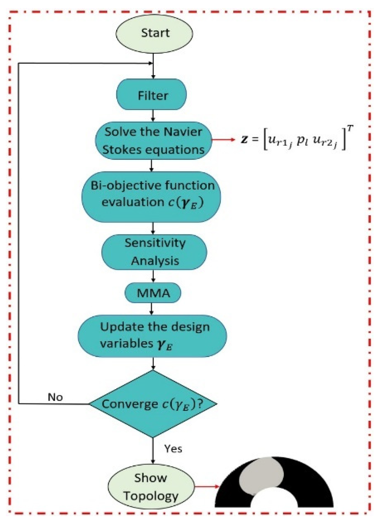Figure 3 shows the topological optimization algorithm implemented in this research.

3.6.1. Sensitivity Analysis (E.D.)

It is also possible to analytically determine the gradient of the energy dissipation functions, as is shown in Equations (36) and (37). At this point, it is highlighted that the energy dissipation function is expanded by including the pressure state design variable through $z={\left[u_{{r1}_j} p_l u_{{r2}_j}\right]}^T$ to achieve compatibility with the resulting equation from the residual:

$${\displaystyle \frac{d{c}_d\left({\gamma }_E\right)}{d{\gamma }_E}}={\displaystyle \frac{1}{2}}{\mathit{z}}^T{\displaystyle \frac{\partial \left({\mathit{k}}^E\left({\gamma }_E\right)\right)}{\partial {\gamma }_E}}\mathit{z}-{\mathit{\lambda }}_d^T{\displaystyle \frac{\partial \mathit{R}}{\partial {\gamma }_E}}$$

(36)

$$\mathit{J}{\mathit{\lambda }}_{Cd}={\left[\left({\mathit{k}}^E\left({\gamma }_E\right)\mathit{z}\right)\right]}^T$$

(37)

where:

${\displaystyle \frac{d{c}_d\left({\gamma }_E\right)}{d{\gamma }_E}}$ → vector of total derivatives;

$z$ → state variable vector;

${\displaystyle \frac{\partial \left({\mathit{k}}^E\left({\gamma }_E\right)\right)}{\partial {\gamma }_E}}$ → vector of explicit derivatives;

${\mathit{\lambda }}_{Cd}$ → adjoint vector;

$\mathit{R}$ → residual vector of the FEM equations.

3.6.2. Sensitivity Analysis (V)

Applying the same method in the previous section, the sensitivities of the vorticity function with respect to the design variable are also calculated, and these sensitivities are shown in Equations (38) and (39).

$${\displaystyle \frac{d{c}_r\left({\gamma }_E\right)}{d{\gamma }_E}}=-{\mathit{\lambda }}_r^T{\displaystyle \frac{\partial \mathit{R}}{\partial {\gamma }_E}}$$

(38)

$$\mathit{J}{\mathit{\lambda }}_r=\left({\mathit{M}}_{\mathit{r}}+{{\mathit{M}}_{\mathit{r}}}^T\right){\left[{\mathit{u}}_{\mathit{r}},\mathbf{0}\right]}^T$$

(39)

where:

${\displaystyle \frac{d{c}_r\left({\gamma }_E\right)}{d{\gamma }_E}}$ → vector of total derivatives of the vorticity;

${\mathit{\lambda }}_r$ → adjoint vector of the vorticity;

$J$ → Jacobian matrix;

${\mathit{M}}_{\mathit{r}}$ → Vorticity matrix.

The explicit derivative in Equation (38) is zero because it only depends on the diffusive terms in the Navier–Stokes equation, which do not depend on the design variable. Additionally, it should be mentioned that, to guarantee the compatibility of the left and right sides in Equation (39), the adjoint vector is calculated by direct selection. For example, for the column vector ${\left[{\mathit{u}}_{\mathit{r}},\mathbf{0}\right]}^{\mathit{T}}$ of one element, the nodal solutions of the velocities at x₁ and x₂ are chosen, omitting the nodal results of the pressures and generating a column vector of 16 × 1 of dimensions for the adjoint vector.

3.7. Filter

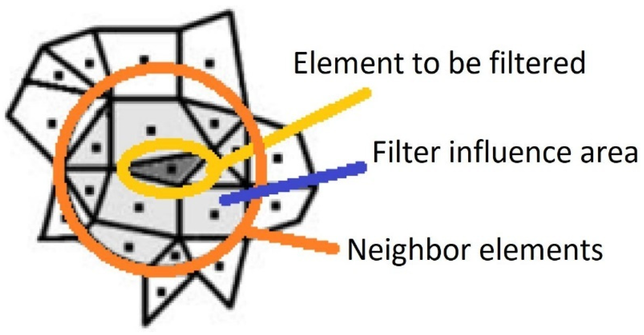
The mesh dependence problem is reduced with the application of spatial filters, since they control the area of influence from a defined radius (R_max), resulting in control of the topology complexity [25]. Figure 4 illustrates the concept of a spatial filter in a two-dimensional mesh, where the element being filtered has a neighborhood selected by the radius of the filter R_max. Neighboring elements are those where the centroid of these elements is within the filter’s area of influence.

The filter used in this paper is the one proposed by Cardoso and Fonseca [25]. The formulation of this filter is detailed in Equation (40), and it is called an average weight spatial filter (AWSF):

$${\widehat{a}}_{ i}={\displaystyle \frac{a_i{V}_i+{\overline{W}}_{ i}{\sum }_{j=1}^{nv}{a}_j{V}_j}{V_i+{\overline{W}}_{ i}{\sum }_{j=1}^{nv}{V}_j}}, {\overline{W}}_{ i}=\sum _{j=1}^{nv}{\displaystyle \frac{R_{max}-R_{ij}}{nv\ast R_{max}}}$$

(40)

where:

$a_i$ is the value of the variable without filter;

$V_i$ is the volume of the element i;

$W$ is a weight factor;

$\overline{W}$ is an average value of the weight factor;

$R_{max}$ is the radius of the filter;

$R_{ij}$ is the distance between the center of element i and the center of element j;

$nv$ is the number of neighboring elements.

4. Parallel Computing in the Cloud

Modern engineering requires significant computational capabilities in different areas of expertise, as engineering processes have become more complex and need frequent improvements. In this paper, parallel computing in the cloud is proposed as a platform solution to solve the TOM and FEM and applied is to flow problems in centrifugal pumps.

For decades, researchers in computational fluid dynamics have developed numerical methods to formulate and solve mathematical problems related to the physics of flow problems. These numerical methods can be classified into two main groups, such as “conventional methods” and “accelerated methods” [27,28,29,30,31,32,33].

Conventional methods are the most widely used method, highly accurate, and used in most commercial packages (Ansys Fluent, Abaqus, etc.). However, conventional methods may occupy more computational memory when solving the fluid field in a certain design domain. For example, based on D. Kandhai et al. [34], the Lattice–Boltzman method (LBM) uses 10 times less memory compared to the MEF when solving for flow in static mixer reactors, making it almost impossible to solve large problems in a reasonable time. On the other hand, accelerated methods are categorized into two main groups: advanced numerical methods and hardware techniques. The hardware techniques are generally used in conjunction with conventional and advanced numerical methods [27]. The hardware techniques are used in this paper in conjunction with FEM as a solution technique to obtain the design of blades in turbomachinery. The interface tool chosen in this paper as a parallelization technique is the “Parallel Computing Toolbox” provided by MATLAB, which allows the user to select the number of “workers” or “cores” required to execute the algorithm.

4.1. CPU Architectures Selected in the Cloud for Execution of the Algorithm in Parallel

In this research, to accelerate the design process of the blade in a centrifugal pump, a virtual machine is used in Amazon Web Services (AWS) and a bare-metal machine in the EQUality, Neutrality and Internet eXchange (Equinix). The providers of these CPUs offer computer rental per hour to an end user, who remotely accesses these supercomputers through a personal computer and internet access. The two types of servers in the cloud (bare-metal and virtual machine) have a physical server that will be located at the provider’s facilities. The difference between these two terms lies clearly in the way the providers manage this server for the rental of these resources to the end user (s). In the bare-metal service, the entire physical server is dependent upon a single user. Therefore, the user has total control of the entire server for the proper management of the computational resources. On the other hand, in a virtual machine, the provider will virtualize this physical server (through a hypervisor) to create several virtual machines, so that several users can access these shared resources (RAM, cores, GPU, etc.) from the same server.

4.1.1. Virtual Machine in AWS

Table 1. Characteristics of the type of processor used in the virtual machine for the parallelized TOM algorithm.

Provider	Instance/Server name	Processor	Vcpus	Clock Speed (GHz)	City-Country
AWS	M5ad.12xlarge	AMD EPYC 7571	48	2.2	Seattle, WA, USA

, characteristics of the type of processor used in the virtual machine for the parallelized TOM algorithm, specifies the type of processor used in the virtual machine to measure the performance of the parallelized TOM algorithm in the cloud.

The architecture of this type of processor is shown in Figure 5. This processor offers a speed on each core of 2.2 GHz, where there is a communication channel (data/address bus) with the RAM.

4.1.2. Bare-Metal Machine in Equinix

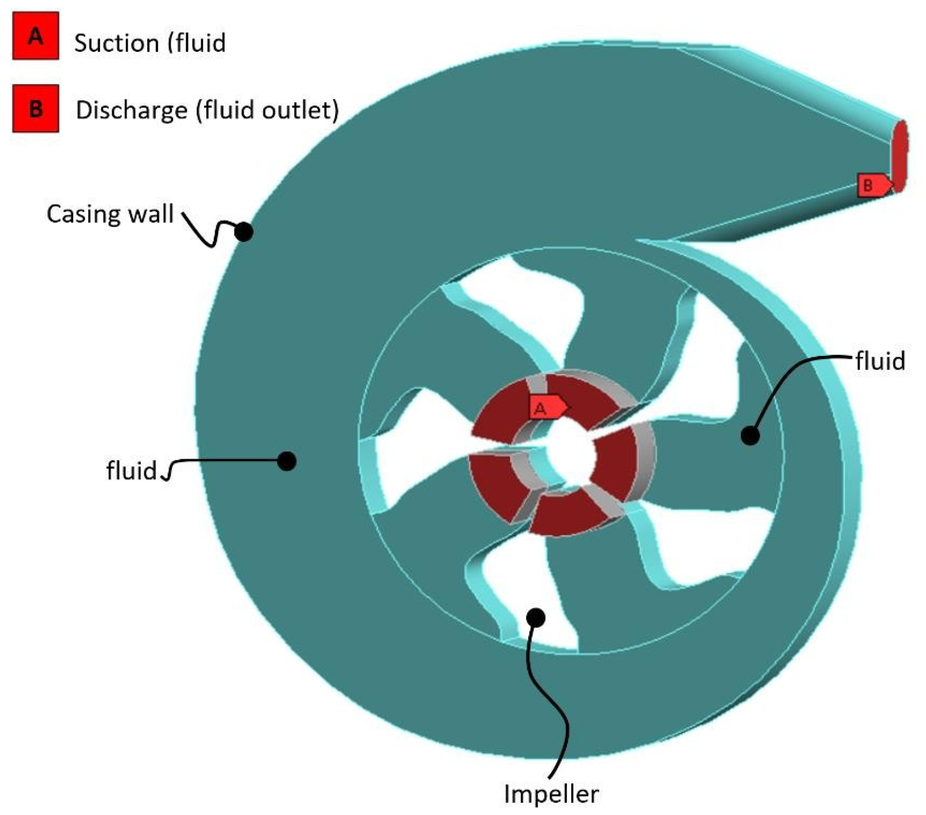
The provider selected for the bare-metal machine is Equinix (

Table 2. Characteristics of the type of processor used in Equinix.

Provider	Instance/Server Name	Processor	Cores	Clock Speed (GHz)	City-Country
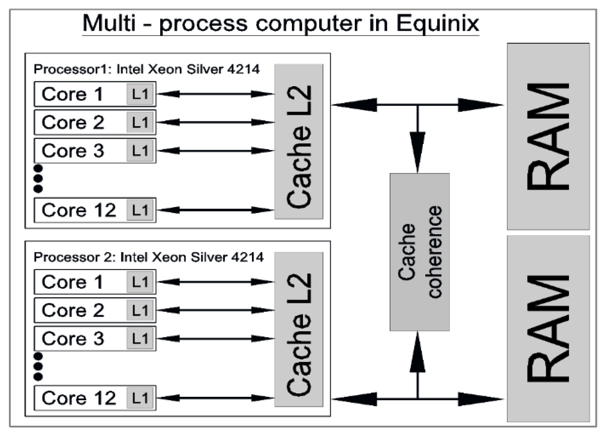
Equinix	s3.xlarge.x86	Intel Xeon Silver	14	2.2	Redwood, CA, USA

). The server has two scalable processors interconnected with each other. This processor consists of 12 physical cores. That is, a total of 24 resource cores can be used in this supercomputer.

The architecture of this processor is shown in Figure 6. This processor shows scalable technology that works with more than one multi-core processor. That is, each processor is placed in its own socket.

5. Results

5.1. FEM Code Verification—Viscous Flow

Before running the TOM algorithm for the design of the blade in centrifugal pumps, it is necessary to perform the verification of the FEM. Therefore, the straight blade of Figure 7 is considered in order to work with a Newtonian flow that enters through the inlet condition with a uniform velocity of magnitude 1 [m/seg]. The remaining boundary conditions are the walls (45° separated between them) and the outlet condition with a gauge pressure of 0 [Pa]. The parameters for the FEM simulation are presented in

Table 3. Straight-blade simulation parameters.

Parameters	Value
Fluid	Generic
State	Stationary
Kinematic Viscosity	0.1 [kg/m·s]
Fluid density	1 [kg/m3]
Inlet Velocity	1 [m/s]
Outlet pressure	0 [Pa]
Angular velocity	1000 r.p.m

:

The velocity and pressure contours are plotted in MATLAB version R2020a and are verified numerically with the commercial software ANSYS FLUENT version 18.2 (Figure 8 and Figure 9). The fluid contours are globally modeled with localized variations that can be caused by differences in the convergence criteria by an algorithm, by a type of finite element, and, in the case of the commercial software, by differences in formulation.

5.2. TOM Model for Turbomachines

The design domain is considered a half rotor, as shown in Figure 10. It is observed that there is a two-dimensional model in which there is a fluid with a velocity at the inlet and a pressure at the outlet. This uniform velocity at the inlet is normal to the curve of the internal radius. This model is a simplification of the assumption of a fluid flow between two consecutive blades in the rotor of a centrifugal pump. The parameters for the design problem of the rotor using TOM are shown in

Table 4. Parameters of the turbomachinery rotor design problem using TOM.

Fluid Field Parameters
Parameter	Value
Fluid	Generic
State	Stationary
Kinematic viscosity	0.1 [kg/m·s]
Fluid density	1 kg/m3
Inlet velocity	1 m/s
Outlet pressure	0 Pa
Angular velocity	1000 r.p.m.
Permeability penalty	1
Maximum Brinkman’s penalty	1 × 105
Minimal Brinkman’s penalty	0
TOM parameters
Objective volume function	0.25
Optimization method	MMA
Number of finite elements	1.800
Initial pseudo-density	0.25

. It is noteworthy that the permeability penalty is a parameter that must be chosen between 0.01 and 1. Values greater than one restrict the search space in the minimization of the objective function.

The result of the topology optimization obtained by minimizing the energy dissipation is shown in Figure 11, and the convergence curve of the MMA algorithm is shown in Figure 12. Figure 11 shows that the material model implemented in Equation (27) is strong enough to adequately represent the solid as an impermeable fluid. The gray scales (intermediate design variables) in the upper left side represent neither a solid nor a fluid. That is, they do not have a physical representation. These gray scales are attributed to a very large filter radius. On the other hand, Figure 12 depicts that the convergence in the energy dissipation minimization is reached quickly. That is, with barely any iterations. This rapid convergence is because this parameter does not present peaks in the minimization of this function. Moreover, the sensitivities reach a local minimum very quickly, and these gradients begin to stabilize. It can also be observed that the target volume restriction of 0.25 is violated in the first iterations, but after the #5 iteration, it begins to decrease and then stabilizes. The performance obtained in this minimization of the energy dissipation was 5.9 [Watts], with a fraction volume in the whole domain of 0.248.

5.2.1. TOM Bi-Objective Function: Minimization of Energy Dissipation and Vorticity

For this bi-objective function, it is necessary to regard a distributed weight, considering that the sum of them is equal to one (wd + wr = 1). In this work, we consider a weight of w_d = 0.8 for the energy dissipation and a weight of w_r = 0.2 for the vorticity. Figure 13 shows the influence that vorticity has on the result of the topology, presenting a section with less radius of curvature. That is, a less hydrodynamic profile, thus obtaining less abrupt sections where the fluid will flow and inducing it to experiment with less rotation, which leads to a minimization of vorticity throughout the design domain. Figure 14 depicts that there are more iterations for its convergence because it has two functions, resulting in a greater delay for the stabilization of its gradients when finding the local optimum.

5.2.2. Post-Processing of Turbomachine Rotors

Figure 15 shows the blade in a complete circumference, simulating the impeller of a centrifugal pump. Moreover, it shows the open rotors built with a five-blade design for topologies of each of the following cases: (a) case 1: mono-objective function minimization of energy dissipation (w_d = 1 and w_r = 0) and (b) case 2: bi-objective function minimization of energy dissipation and vorticity (w_d = 0.8 for the energy dissipation and w_r = 0.2). The choice of five blades on the rotor is given because it is the maximum number that will fit in a complete circumference.

The rotor design is complemented with the inclusion of a casing, where the fluid portions that correspond to the interior of the pump can be seen in Figure 16. The impeller selected for this model corresponds to case 1, where water is considered as fluid, with an inlet velocity of 1 [m/seg] in the suction section (equivalent to a mass flow at the inlet of 0.12 [kg/seg] and an outlet pressure of 0 [Pa] at the discharge section. The peripheral section of the casing is considered to be a wall with an assigned constant angular velocity of 1.815 rpm.

To verify the topologies previously obtained, the rotor is extended to the entire circumference (Figure 17), where a 3D model is simulated in ANSYS Fluent software. The minimization of energy dissipation (left figure) was prioritized, obtaining a total pressure of 3.90 [GPa] and a vorticity of 8.36 × 10⁷ [1/s]. And, in the right-side figure, the minimization of the bi-objective function is prioritized, obtaining a lower vorticity of 5.40 × 10⁷ [1/s] in the whole domain, representing 35% less compared to the other rotor.

5.3. Performance of the Serial and Parallel Computational Algorithms Using Cloud Computing

In this section, we decided to evaluate the computational algorithm for the design of blades in turbomachines in terms of scalability and efficiency.

5.3.1. Performance of the FEM and TOM Algorithm for Case 1: Mono-Objective Function, Minimization of Energy Dissipation (w_d = 1 and w_r = 0)

Figure 18 shows the scalability graphs (acceleration vs. number of processors) for both of the machine’s CPU architectures. The AWS graph shows that the speed-ups obtained are 3.88x, 5.99x, 6.25x, 6.69x, 7.18x, and 7.48x, when using 4, 8, 12, 16, 20, and 24 cores in parallel, respectively. On the other hand, the Equinux graph shows that the speed-ups obtained for this type of architecture are 4.02x, 5.95x, 6.74x, 6.80x, and 6.80x, for the same number of cores.

It could be thought that these speed-ups are not very favorable for obtaining the final design of the blade. But, if we compare the time in series for the virtual machine in AWS (13,033 [sec] equal to 3.62 h) and in Equinix (9646 [sec] equal to 2.67 h) with the time in parallel when using 24 cores (1741 [sec] equal to 29 [min] in AWS and 1418 [sec] equal to 23 min and 37 s in Equinix), it can be noticed that the design time is greatly reduced, which is a very favorable point that should be taken into account not only at an academic level but at and industrial level, where time is a very important factor in the production of blade-designed turbomachines.

Figure 19 shows the efficiency graphs for both CPU architectures. For AWS, the efficiencies obtained are 0.97, 0.75, 0.52, 0.42, 0.36, and 0.31 when using 4, 8, 16, 20, and 24 cores, respectively. On the other hand, for Equinix, the efficiencies obtained are 1.01, 0.74, 0.56, 0.42, 0.34, and 0.28 for the same numbers of cores.

5.3.2. Performance of the FEM and TOM Algorithm for Case 2: Bi Objective Function: Minimization of Energy Dissipation and Vorticity (w_d = 0.8 and w_r = 0.2)

Figure 20 shows the scalability (acceleration vs. number of processors) for both of the machine’s CPU architectures. For the AWS, the speed-ups obtained are 3.84x, 5.93x, 6.27x, 6.68x, 7.14x, and 7.49x when using 4, 8, 12, 16, 20, and 24 cores in parallel, respectively. On the other hand, for Equinix, the speed-ups obtained for this architecture are 4.02x, 5.83x, 6.61x, 6.74x, and 6.72x for the same number of cores. These speed-ups are very similar to case I for both AWS and Equinix, due to the similarity in the algorithms, with the only difference being that the weight distributions vary, resulting in convergence in different numbers of iterations.

Figure 21 shows the efficiency for both CPU architectures. For AWS, the efficiencies obtained are 0.96, 0.74, 0.52, 0.42, 0.36, and 0.31 when using 4, 8, 16, 20, and 24 cores, respectively. On the other hand, for Equinix, the efficiencies obtained are 1.01, 0.73, 0.55, 0.42, 0.34, and 0.29 for the same number of cores.

6. Discussions and Conclusions

Topological optimization of fluids using the finite-element method has attracted the attention of many researchers due to its ability to design optimal geometries in fluid transport and control systems. Among the pioneering works, Borrvall and Petersson (2003) developed a general framework for optimizing flow in two-dimensional systems, using formulations based on the Stokes equation [16]. In their results, they demonstrated how it is possible to generate optimal designs to minimize energy dissipation in flow channels. Fonseca et al. extended the approach by including additional constraints related to structural robustness and fluid–structure interaction [25]. Their studies evidenced that the integration of multiple objectives in the optimization allows for obtaining designs that not only maximize hydraulic performance but also guarantee mechanical stability. Compared to Borrvall and Petersson’s work, the optimized geometries presented more complex configurations but with a significant improvement in energy efficiency and wear resistance. On the other hand, Brenner explored topological optimization in three-dimensional systems using improved finite-element methods to handle the increased computational complexity. The results showed that optimized three-dimensional configurations allow for more precise flow control, especially in applications such as heat exchangers and microfluidic systems. Compared to two-dimensional approaches, three-dimensional designs offer advantages in specific industrial applications, although they require a higher computational cost. Hosain and Cardoso took an innovative approach by incorporating nonlinear effects in flow optimization, extending applications to the turbulent regime [25,27]. Their research highlighted how advanced formulations based on the Navier–Stokes equation allow systems with high velocity flows and higher complexity to be optimized. In their results, they achieved designs that improved hydraulic efficiency by 20–30% compared to traditional methods, showing the potential of topological optimization in real systems.

The purpose of this article is to show the reader that there are mathematical optimization tools that, although they take time to implement to a specific problem, can save costs and time at the design time. The result of obtaining a lower vorticity is an important issue, especially in ventricular assist devices where a minimization of this physical phenomenon is required. In this work, the minimization of energy dissipation and increased vorticity could increase the hydraulic efficiency by 38%, which is similar to what Hosain and Cardoso stated.

Techniques such as cloud computing allow for the development of a parallelized topological optimization algorithm, obtaining designs for turbomachinery rotors that may be non-intuitive for the designer. Similarly, the parallelization of the computational algorithm in the design model of “blades in half-rotor circumference’’ is considered successful. The fact of reducing the execution time to more than half increases the robustness of the developed algorithm. These parallelization techniques (bare metal and virtual machine) are one of the accelerated-method techniques that were studied in this paper and that motivate other readers to continue investigating new techniques to reduce the computational costs that we face today.

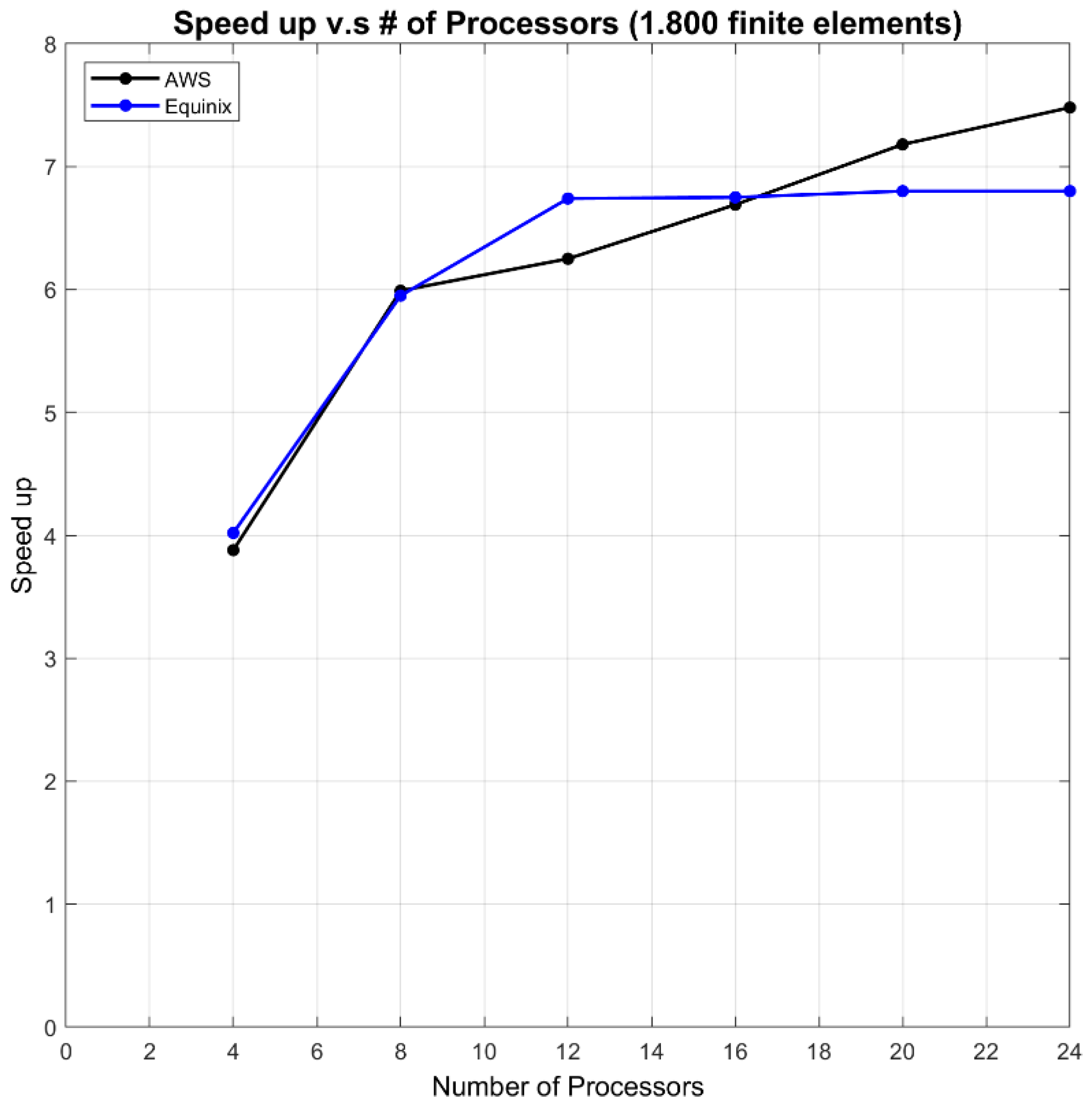
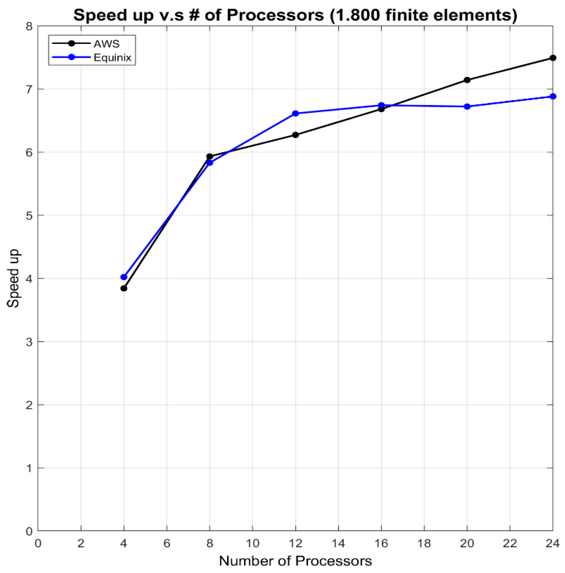
For this specific problem (design of rotors in half circumference), it is recommended to use AWS if it is required to execute the TOM algorithm in serial or with the use of four cores in parallel. On the other hand, for greater than four cores, it is recommended to run the algorithm in Equinix, due to the costs per hour that each provider charges for their respective services.

The Brinkman material model penalty is strong enough to represent solid and fluid zones, resulting in topologies that represent the physical minimization of the problem. The methodology used allows for extending the study of other objective functions of the turbomachine design problem. This study can go beyond hydrodynamics and, thus, be extended to objective structural functions that analyze the mechanical parts that comprise it, for example, the study of the stresses generated in the rotor of a turbomachine through interaction with the fluid.

In summary, topological optimization has proven to be a successful method for the design of rotors of radial flow machines. The work of several authors has established a solid foundation for the topological optimization of fluids using finite elements, ranging from basic formulations to advanced applications in three-dimensional contexts and with turbulence. Although each approach has specific advantages depending on the conditions of the problem, all agree that this technique offers great potential to improve the efficiency and functionality of flow systems, consolidating itself as a key tool in modern engineering.

References

1. Aaronson, K.D.; Slaughter, M.S.; Miller, L.W.; McGee, E.C.; Cotts, W.G.; Acker, M.A.; Jessup, M.L.; Gregoric, I.D.; Loyalka, P.; Frazier, O.H.; et al. Use of an intrapericardial, continuous-flow, centrifugal pump in patients awaiting heart transplantation. Circulation 2012, 125, 764–775. [Google Scholar]
2. Cheah, K.W.; Lee, T.S.; Winoto, S.H.; Zhao, Z.M. Numerical flow simulation in a centrifugal pump at design and off-design conditions. Int. J. Rotating Mach. 2007, 2007, 083641. [Google Scholar] [CrossRef]
3. Jafarzadeh, B.; Hajari, A.; Alishahi, M.M.; Akbari, M.H. The flow simulation of a low-specific-speed high-speed centrifugal pump. Appl. Math. Model. 2011, 35, 242–249. [Google Scholar]
4. Dong, L.; Zhang, Y.; Ge, Z.; Dai, C.; Guo, J. Study and Verification of Large-Scale Parallel Mesh Generation Algorithm for Centrifugal Pump. Math. Probl. Eng. 2020, 2020, 1956852. [Google Scholar]
5. Nocente, A.; Arslan, T.; Jasiński, D.; Nielsen, T.K. A study of flow inside a centrifugal pump: High performance numerical simulations using GPU cards. In Proceedings of the Open Archives of the 16th International Symposium on Transport Phenomena and Dynamics of Rotating Machinery, Honolulu, HI, USA, 10–15 April 2016. [Google Scholar]
6. Derakhshan, S.; Pourmahdavi, M.; Abdolahnejad, E.; Reihani, A.; Ojaghi, A. Numerical shape optimization of a centrifugal pump impeller using artificial bee colony algorithm. Comput. Fluids 2013, 81, 145–151. [Google Scholar]
7. Li, W.G. Inverse design of impeller blade of centrifugal pump with a singularity method. Jordan J. Mech. Ind. Eng. 2011, 5, 119–128. [Google Scholar]
8. Tan, L.; Cao, S.; Wang, Y.; Zhu, B. Direct and inverse iterative design method for centrifugal pump impellers. Proc. Inst. Mech. Eng. Part A J. Power Energy 2012, 226, 764–775. [Google Scholar]
9. Gölcü, M.; Pancar, Y.; Sekmen, Y. Energy saving in a deep well pump with splitter blade. Energy Convers. Manag. 2006, 47, 638–651. [Google Scholar]
10. Zhao, W.; Sheng, J.; Yang, J.; Song, Q. Optimization design and experiment of centrifugal pump based on CFD. Nongye Gongcheng Xuebao/Trans. Chin. Soc. Agric. Eng. 2015, 31, 125–131. [Google Scholar]
11. Wang, W.; Pei, J.; Yuan, S.; Zhang, J.; Yuan, J.; Xu, C. Application of different surrogate models on the optimization of centrifugal pump. J. Mech. Sci. Technol. 2016, 30, 567–574. [Google Scholar]
12. Wang, C.; Feng, Y.; Ye, J.; Luo, B.; Liu, K. Multi-objective parameters optimization of centrifugal slurry pump based on RBF neural network and NSGA-II genetic algorithm. Nongye Gongcheng Xuebao/Trans. Chin. Soc. Agric. Eng. 2017, 33, 109–115. [Google Scholar]
13. Toteff, J.; Tovar Asuaje, M.A. Design and multiparameter optimization of jet-pumps in a pipeline loops using CFD tools. In Proceedings of the American Society of Mechanical Engineers Fluids Engineering Division Summer Meeting (FEDSM), Montreal, QC, Canada, 15–20 July 2018; Volume 2. [Google Scholar]
14. Rhyu, S.H.; Kumar, S.; Khaliq, S.; Yoon, M.H.; Yun, J.E.; Lee, S.S. Design optimization for pullout torque improvement of a magnetic coupling in chemical pump application. J. Magn. 2021, 26, 60–66. [Google Scholar] [CrossRef]
15. Blommaert, M.; Wack, Y.; Baelmans, M. An adjoint optimization approach for the topological design of large-scale district heating networks based on nonlinear models. Appl. Energy 2020, 280, 116025. [Google Scholar] [CrossRef]
16. Borrvall, T.; Petersson, J. Topology optimization of fluids in Stokes flow. Int. J. Numer. Methods Fluids 2003, 41, 77–107. [Google Scholar] [CrossRef]
17. Romero, J.S.; Silva, E.C.N. A topology optimization approach applied to laminar flow machine rotor design. Comput. Methods Appl. Mech. Eng. 2014, 279, 268–300. [Google Scholar] [CrossRef]
18. Sá, L.F.N.; Romero, J.S.; Horikawa, O.; Silva, E.C.N. Topology optimization applied to the development of small scale pump. Struct Multidisc Optim 2018, 57, 2045–2059. [Google Scholar] [CrossRef]
19. Chang, H.; Yang, J.; Wang, Z.; Peng, G.; Lin, R.; Lou, Y.; Shi, W.; Zhou, L. Efficiency optimization of energy storage centrifugal pump by using energy balance equation and non-dominated sorting genetic algorithms-II. J. Energy Storage 2025, 114 Pt B, 115817. [Google Scholar] [CrossRef]
20. White, F.M. Fluid Mechanics, 7th ed.; McGraw-Hill: New York, NY, USA, 2011. [Google Scholar]
21. Kundu, P.K.; Cohen, I.M. Fluid Mechanics; McGraw-Hill: New York, NY, USA, 2008; Volume 10. [Google Scholar]
22. Bastidas, X.A.; Montealegre-Rubio, W. Design of rotors in centrifugal pumps using the topology optimization method. In Proceedings of the 2021 14th IEEE International Conference on Industry Applications (INDUSCON), São Paulo, Brazil, 15–18 August 2021; pp. 126–133. [Google Scholar] [CrossRef]
23. Cengel, Y.A.; Cimbala, J.M. Fluid Mechanics: Fundamentals and Applications, 4th ed.; McGraw-Hill: New York, NY, USA, 2020; Volume 91. [Google Scholar]
24. Reddy, J.N.; Gartling, D.K. The Finite Element Method in Heat Transfer and Fluid Dynamics, 3rd ed.; CRC Press: Boca Raton, FL, USA, 2010. [Google Scholar]
25. Fraser, W.H. Flow Recirculation in Centrifugal Pumps. Water Eng. Manag. 1985, 132, 95–100. [Google Scholar]
26. Gürdal, Z.; Haftka, R.T. Sensitivity derivatives for static test loading boundary conditions. AIAA J. 1985, 23, 159–160. [Google Scholar] [CrossRef]
27. Cardoso, E.L.; Fonseca, J.S.O. Complexity control in the topology optimization of continuum structures. J. Braz. Soc. Mech. Sci. Eng. 2003, 25, 293–301. [Google Scholar] [CrossRef]
28. Hurtado-Pérez, A.B.; Pablo-Sotelo, A.D.J.; Ramírez-López, F.; Hernández-Gómez, J.J.; Mata-Rivera, M.F. On Topology Optimisation Methods and Additive Manufacture for Satellite Structures: A Review. Aerospace 2023, 10, 1025. [Google Scholar] [CrossRef]
29. Hosain, M.L.; Fdhila, R.B. Literature Review of Accelerated CFD Simulation Methods towards Online Application. Energy Procedia 2015, 75, 3307–3314. [Google Scholar] [CrossRef]
30. Christiansen, I.P. Numerical simulation of hydrodynamics by the method of point vortices. J. Comput. Phys. 1973, 13, 363–379. [Google Scholar] [CrossRef]
31. Buneman, O. Dissipation of currents in ionized media. Phys. Rev. 1959, 115, 503. [Google Scholar] [CrossRef]
32. Brenner, T.A.; Fontenot, R.L.; Cizmas, P.G.A.; O’Brien, T.J.; Breault, R.W. A reduced-order model for heat transfer in multiphase flow and practical aspects of the proper orthogonal decomposition. Comput. Chem. Eng. 2012, 43, 68–80. [Google Scholar] [CrossRef]
33. Harlow, F.H.; Welch, J.E. Numerical calculation of time-dependent viscous incompressible flow of fluid with free surface. Phys. Fluids 1965, 8, 2182. [Google Scholar] [CrossRef]
34. Kandhai, D.; Vidal, D.J.E.; Hoekstra, A.G.; Hoefsloot, H.; Iedema, P.; Sloot, P.M.A. Lattice-Boltzmann and finite element simulations of fluid flow in a SMRX static mixer reactor. Int. J. Numer. Methods Fluids 1999, 31, 1019–1033. [Google Scholar] [CrossRef]
Figure 1. Radial impeller blade geometry profile. Montealegre et al. (2021) [22].
Machines 13 00307 g001
Figure 2. Scheme of the design problem for turbomachine rotors regarding global coordinates, for the implementation of the finite-element method. Montealegre et al. (2021) [22].
Machines 13 00307 g002
Figure 3. Flowchart of the topology optimization algorithm.
Machines 13 00307 g003
Figure 4. Concept of spatial filter in a bidimensional mesh [26].
Machines 13 00307 g004
Figure 5. CPU architecture used in AWS; 2.2 GHz core speed.
Machines 13 00307 g005
Figure 6. CPU architecture used in Equinix. 2.2 GHz core speed.
Machines 13 00307 g006
Figure 7. Straight blade, dimensions, and boundary conditions.
Machines 13 00307 g007
Figure 8. Velocity contour for the viscous flow problem used for verification of the FEM code. (a) Implemented code in Matlab, (b) commercial software (ANSYS Fluent), (c) Romero et al. (2014) [17].
Machines 13 00307 g008
Figure 9. Pressure contour for the viscous flow problem used for verification of the FEM code. (a) Implemented code in MATLAB, (b) Commercial software (ANSYS FLUENT), (c) Romero and Silva (2014) [17].
Machines 13 00307 g009
Figure 10. Scheme of the design problem for turbomachine rotors using TOM. Montealegre et al. (2021) [22].
Machines 13 00307 g010
Figure 11. Topology optimization result for energy dissipation wd = 1 and wr = 0, considering yini = 0.25 throughout the design domain with 1800 finite elements for the design of turbomachine rotors. Montealegre et al. (2021) [22].
Machines 13 00307 g011
Figure 12. Convergence curve minimizing the energy dissipation (wd = 1 and wr = 0) for the design of turbomachine rotors.
Machines 13 00307 g012
Figure 13. Topology optimization result for the bi-objective function with wd = 0.8 for the energy dissipation and wr = 0.2 for the vorticity, considering yini. = 0.25 throughout the design domain with 1800 finite elements for the design of turbomachine rotors.
Machines 13 00307 g013
Figure 14. Convergence curve minimizing the bi-objective function (wd = 0.8 for the energy dissipation and wr = 0.2) for the design of turbomachine rotors.
Machines 13 00307 g014
Figure 15. Impeller design for the small-scale centrifugal pump model considering 5 blades: (a) case 1: mono-objective function: minimization of energy dissipation (wd = 1 and wr = 0) and (b) case 2: bi-objective function: minimization of energy dissipation and vort.
Machines 13 00307 g015
Figure 16. Small-scale centrifugal pump model for the impeller in case 1: mono-objective function minimization of energy dissipation (wd = 1 and wr = 0).
Machines 13 00307 g016
Figure 17. Pressure field for the problem of small-scale pump rotors. (left) Total pressure: 3.90 [GPa] and vorticity: 8.36 × 10⁷ [1/s]. (right) Total pressure: 2.40 [GPa] and vorticity: 5.40 × 10⁷ [1/s].
Machines 13 00307 g017
Figure 18. Scalability, speed-up vs. number of processors for 1800 finite elements in the design model of blades in turbomachines in half rotor circumference for case I.
Machines 13 00307 g018
Figure 19. Efficiency vs. number of processors for 1800 finite elements in the design model of blades in turbomachines in half rotor circumference for case 1.
Machines 13 00307 g019
Figure 20. Scalability, speed-up vs. number of processors for 1800 finite elements in the design model of blades in turbomachines in half rotor circumference for case II: bi-objective function.
Machines 13 00307 g020
Figure 21. Efficiency vs. number of processors for 1800 finite elements in the design model of blades in turbomachines in half rotor circumference for case II.
Machines 13 00307 g021