Surface Classification from Robot Internal Measurement Unit Time-Series Data Using Cascaded and Parallel Deep Learning Fusion Models

Abstract

Surface classification is critical for ground robots operating in diverse environments, as it improves mobility, stability, and adaptability. This study introduces IMU-based deep learning models for surface classification as a low-cost alternative to computer vision systems. Two feature fusion models were introduced to classify the surface type using time-series data from an IMU sensor mounted on a ground robot. The first model, a cascaded fusion model, employs a 1-D Convolutional Neural Network (CNN) followed by a Long Short-Term Memory (LSTM) network and then a multi-head attention mechanism. The second model is a parallel fusion model, which processes sensor data through both a CNN and an LSTM simultaneously before concatenating the resulting feature vectors and then passing them to a multi-head attention mechanism. Both models utilize a multi-head attention mechanism to enhance focus on relevant segments of the time-sequence data. The models were trained on a normalized Internal Measurement Unit (IMU) dataset, with hyperparameter tuning achieved via grid search for optimal performance. Results showed that the cascaded model achieved higher accuracy metrics, including a mean Average Precision (mAP) of 0.721 compared to 0.693 for the parallel model. However, the cascaded model incurred a 44.37% increase in processing time, which makes the parallel fusion model more suitable for real-time applications. The multi-head attention mechanism contributed significantly to accuracy improvements, particularly in the cascaded model.

1. Introduction

With rapid advances in technology, robotics has expanded into almost every field, including education [1], business [2], and healthcare [3]. Terrain detection and classification play a vital role in enabling precise robot control and navigation. Various studies emphasize the advantages of surface classification, such as improving the mobility of walking robots [4], addressing challenges in using intelligent tires based on accelerometers for enhanced mobility [5], and adjusting robot speed according to surface type [6]. Surface detection further helps stabilize legged robots in rough terrain by improving foot placement [7], and supports energy-efficient operating modes [8]. In addition, surface classification can be used to estimate road friction coefficients, contributing to safety improvements [9].

The most common approach to surface classification involves the use of computer vision systems. For example, Iglesias et al. [10] developed a camera-based computer vision system specifically for wood surface classification. Laible et al. [11] presented a robot equipped with a low-resolution 3D LIDAR and color camera to classify the terrain ahead of it. Walas et al. [12] proposed a terrain classification method using a laser rangefinder, where feature vectors were generated through statistical descriptors of the intensity map, with a support vector machine serving as a classifier. Borrmann et al. [13] introduced an autonomous mobile robot that uses both an RGB camera and a thermal camera. An automated 3D crack detection system for structures, achieving high accuracy by fusing LiDAR and a depth camera, was proposed by Hu et al. [14]. Tang et al. proposed visual crack width measurement based on structure backbone double-scale features using machine vision [15].

Inertial Measurement Unit (IMU) sensors are widely utilized in robotics, playing an essential role in various robot applications. For instance, they aid in localization and slip estimation for mobile robots [16], determining the trajectory and direction [17,18], estimating the pose [19], and navigating and localization [20], as well as motion stability control and gait planning [21].

Computer vision faces challenges including sensitivity to lighting variations, high computational demands, and complexities in data acquisition. Traditional vision-based methods rely on extensive labeled datasets and require intricate pre-processing steps [22]. This study addresses the need for a cost-effective approach to surface classification in robotics by utilizing IMU data as an alternative to traditional, higher-cost computer vision systems. Specifically, it utilized two deep learning models—1-D Convolutional Neural Network (CNN) and Long Short-Term Memory (LSTM) networks—to extract meaningful features from time-series IMU data. To further enhance feature quality and improve classification accuracy, a multi-head attention mechanism is incorporated. The study investigates two distinct feature fusion architectures: a cascaded model, where CNN and LSTM are sequentially connected, and a parallel model, where features from both networks are combined simultaneously. Through a comprehensive analysis of classification accuracy and execution runtime, this work compares the strengths and trade-offs of each architecture to offer insights into optimal configurations for low-cost, efficient surface classification in robotic applications.

The paper is organized as follows: Section 2 reviews related work on IMU data applications in robotics using machine learning and deep learning. Section 3 details the proposed model architectures, describing key components and the cascaded and parallel fusion models. Section 4 covers the dataset structure, classes, and the training process. Section 5 explains the evaluation metrics. Section 6 presents classification accuracy and runtime results. Section 7 discusses the findings, including performance trade-offs based on the results. Finally, Section 8 concludes the study by summarizing key insights and suggesting future research directions.

2. Related Work

Various machine learning techniques have been applied to sensor data classification. Giulio et al. [23] investigated the use of decision tree ensembles to detect and localize structural damage in health monitoring systems using vibration sensor data. Kumar et al. [24] developed a human activity recognition system based on smartphone sensor data, employing a random forest algorithm to classify different activities. Al-Refai et al. [25] introduced a system for detecting potholes and analyzing traffic conditions using in-vehicle data, such as speed and acceleration, and tested multiple machine learning algorithms, including Support Vector Machines (SVMs), decision trees, and random forests. Barman and Choudhury [26] applied SVM to classify soil texture based on hydrometer test data. Machine learning algorithms were used in soft robot motion classification [27]. Shirmard et al. [28] provided a comprehensive review of machine learning approaches for processing remote sensing data in mineral exploration.

Recent studies in deep learning have focused on exploring sensor data classification, particularly Recurrent Neural Networks (RNNs), due to their ability to process time-series data effectively. Gupta et al. [29] utilized Convolutional Neural Networks (CNNs) for human activity recognition using data from a single wearable IMU sensor. Qi et al. [30] introduced an LSTM-RNN model comprising a Recurrent Neural Network (RNN), Long Short-Term Memory (LSTM) module, and a dropout layer for classifying multiple hand gestures. Zhu et al. [31] proposed a radar-based human activity recognition system that combines 1-D CNNs and RNNs to analyze radar spectrograms as time-sequential vectors. Al-refai et al. [32] utilized CNN architecture to classify traffic conditions and driving behavior using OnBoard diagnostics data (OBD) and smartphone data. Mekruksavanich et al. [33] conducted a comparative study on the application of LSTM networks for human activity recognition using smartphone sensor data, employing a four-layer CNN-LSTM hybrid architecture. Similarly, Pham et al. [34] investigated LSTM networks for the classification of physiological signals.

The multi-head attention mechanism has been widely employed for data classification tasks. Matar et al. [35] introduced a novel multi-head attention-based Bi-LSTM approach for anomaly detection in multivariate time-series data from wireless sensor networks. Junior et al. [36] designed a multi-head 1-D CNN to identify six types of malfunctions in electric motors using data from two accelerometers. Similarly, Cui et al. [37] proposed a multi-head attention CNN model to enhance fault classification performance in industrial processes by prioritizing the significance of different parameters.

Several research projects have investigated surface classification utilizing time-series deep learning algorithms. For example, Li et al. [38] proposed a surface classification method using a one-dimensional Convolutional Neural Network (1D CNN) followed by a Long Short-Term Memory (LSTM) network, demonstrating superior detection performance compared to baseline algorithms such as XGBoost and Fully Connected Neural Networks (FCNs). Alradaideh et al. [39] further enhanced classification accuracy by employing a CNN with a Bidirectional LSTM (Bi-LSTM) architecture. Feng et al. [40] explored an alternative approach by treating the time series data as an input image for CNN-based feature extraction, followed by LSTM for final feature processing. Jiang et al. [41] introduced a customized convolutional neural network that effectively extracts features from both time and frequency domain representations of the data. This image-based CNN approach outperformed traditional time series algorithms, including decision trees, 1D CNN, and LSTM.

While these studies effectively leverage CNN-LSTM architectures for surface classification, they primarily focus on sequential CNN-LSTM configurations. Furthermore, a critical aspect often overlooked in previous research is the runtime performance and suitability of these algorithms for real-time applications. This study aims to address these limitations by: (1) investigating the impact of different feature fusion strategies, namely cascaded and parallel fusion of 1D CNN and LSTM features; and (2) incorporating a multi-head attention mechanism to enhance model performance, given its limited exploration in IMU time series classification. Additionally, this research comprehensively analyzes the runtime requirements of both proposed models, facilitating a thorough evaluation of their trade-offs in terms of accuracy and computational efficiency.

3. Proposed Deep Learning Model Architecture

Two deep learning models were developed and evaluated in this work to classify the IMU time series data. A one-dimensional (1-D) CNN network, LSTM network, multi-head attention mechanism, and fully connected layer with drop out and softmax layer are utilized to build both models. The key distinction between the two models is how the CNN features and the LSTM features are combined. Section 3.1 explains the model building blocks and algorithms and the architecture of the cascaded feature fusion model and the parallel feature fusion model.

3.1. Model Building Blocks

This section explains the main algorithms we utilized in this work to build our deep learning models for the IMU time series data classification.

3.1.1. 1-D CNN

The One-Dimensional Convolutional Network (1-D CNN) is designed to process sequential data [42]. It is commonly used to extract high-level features from time-series data. In a 1-D CNN, the input sequence is convoluted with a one-dimensional sliding filter. When padding is applied to the input sequence, the output sequence retains the same sequence length. In our implementation, we applied two convolutional layers, consisting of 128 and 64 filters, respectively, with a kernel size of 3 × 1 to capture relevant features. The first layer with 128 neurons ensures that all input sequence features are initially processed without dimensional reduction. The second layer follows a structured reduction approach, where the model progressively compresses and refines the feature representation while maintaining essential information.

3.1.2. LSTM

Long Short-Term Memory (LSTM) is a type of Recurrent Neural Network (RNN) to deal with time series data [43]. The main advantage of the LSTM over the traditional RNN is its ability to deal with long sequences without having vanishing and exploding gradient problems [44]. The LSTM network processes the current input while also considering previous states. As illustrated in Figure 1, the previous states, c^(t−1) and y^(t−1), represent the long-term memory and the short-term memory respectively, while x^(t) represents the current input data. LSTM includes three stages. The first stage is the forget gate, which decides what percentage of long-term memory to remember. The second stage is the input gate, in which the long-term memory is updated based on the previous states and the current input. The last stage is the output gate, which calculates the outputs of the LSTM c^(t) and y^(t), which become the input states for the next iteration. y^(t) from the last time step represents the final output of the LSTM unit.

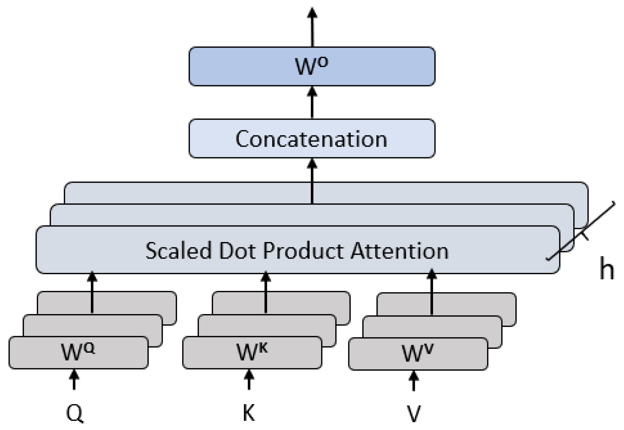
3.1.3. Multi-Head Attention Mechanism

The multi-head attention mechanism is an attention module where the time series input data is divided into multiple partitions and processed in parallel [45]. This mechanism enhances the extraction of richer information from the input by capturing dependencies and relationships across different segments of the sequence. By utilizing multiple attention heads, the module can simultaneously identify and capture diverse patterns within time-series data.

The input data for each head are projected into three spaces, Queries (Q), Keys (K), and Values (V). Q represents a specific time interval in the input data to be focused on. K represents the information about a specific time step in the sequence to identify relationships and dependencies in the time sequence. V Contains the actual values associated with each time step the model will use for module weights update. The architecture of the multi-head attention module is illustrated in Figure 2. The attention mechanism is mathematically defined by Equation (1), and the output of the multi-head attention unit is expressed in Equation (2).

$$\mathrm{Attention}(Q,K,V)=\mathrm{softmax}\left({\displaystyle \frac{Q{K}^T}{\sqrt{d_k}}}\right)V$$

(1)

where:

• Q = Query matrix;
• K = Key matrix;
• V = Value matrix;
• d_k = Dimensionality of the key vectors (for scaling).

$$\mathrm{MultiHead}(Q,K,V)=\mathrm{Concat}({\mathrm{head}}_1,{\mathrm{head}}_2,\dots ,{\mathrm{head}}_h)W^O$$

(2)

where:

• head_i = Attention($Q{W}_i^Q,K{W}_i^K,V{W}_i^V$);
• $W_i^Q,W_i^K,W_i^V$ = learned projection matrices for the i-th head;
• $W^O$ = Learned weight matrix for the output transformation.

Figure 2. Multi-head attention mechanism module architecture.

Figure 2. Multi-head attention mechanism module architecture.

3.2. Feature Fusion Models

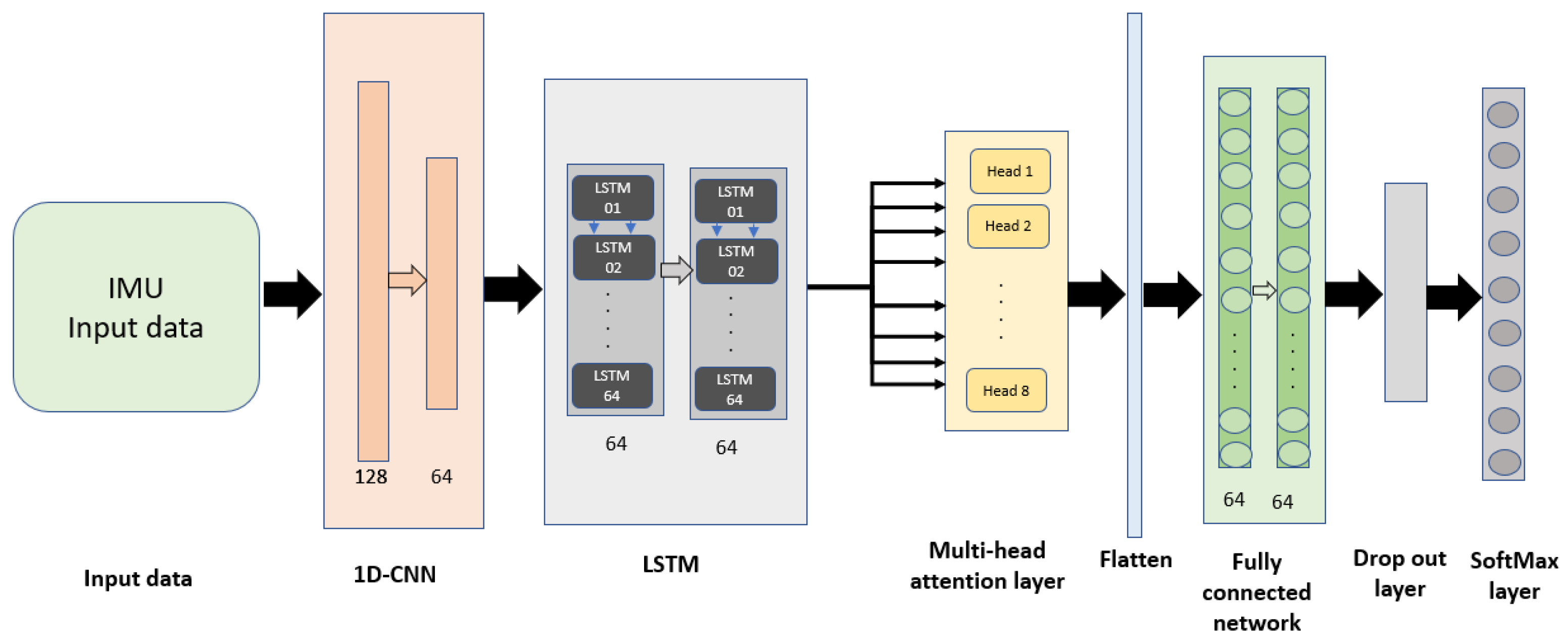
3.2.1. Cascaded Feature Fusion Model

In the cascaded model, IMU data is first fed into a two-layer 1D-CNN to enhance the features of the time series data. The resulting sequences are then passed through a two-layer LSTM network. The final LSTM layer outputs the last time step’s result. The output of the LSTM network is further processed by a muti-head attention mechanism with eight heads, enabling the model to focus on different parts of the time sequence, thereby providing richer information about the data. Finally, the model concludes with a dense network consisting of two layers, followed by a dropout layer and a softmax activation function to classify the time sequence data into the annotated categories. Figure 3 illustrates the architecture for the cascaded feature fusion model, where CNN and LSTM networks are sequentially connected.

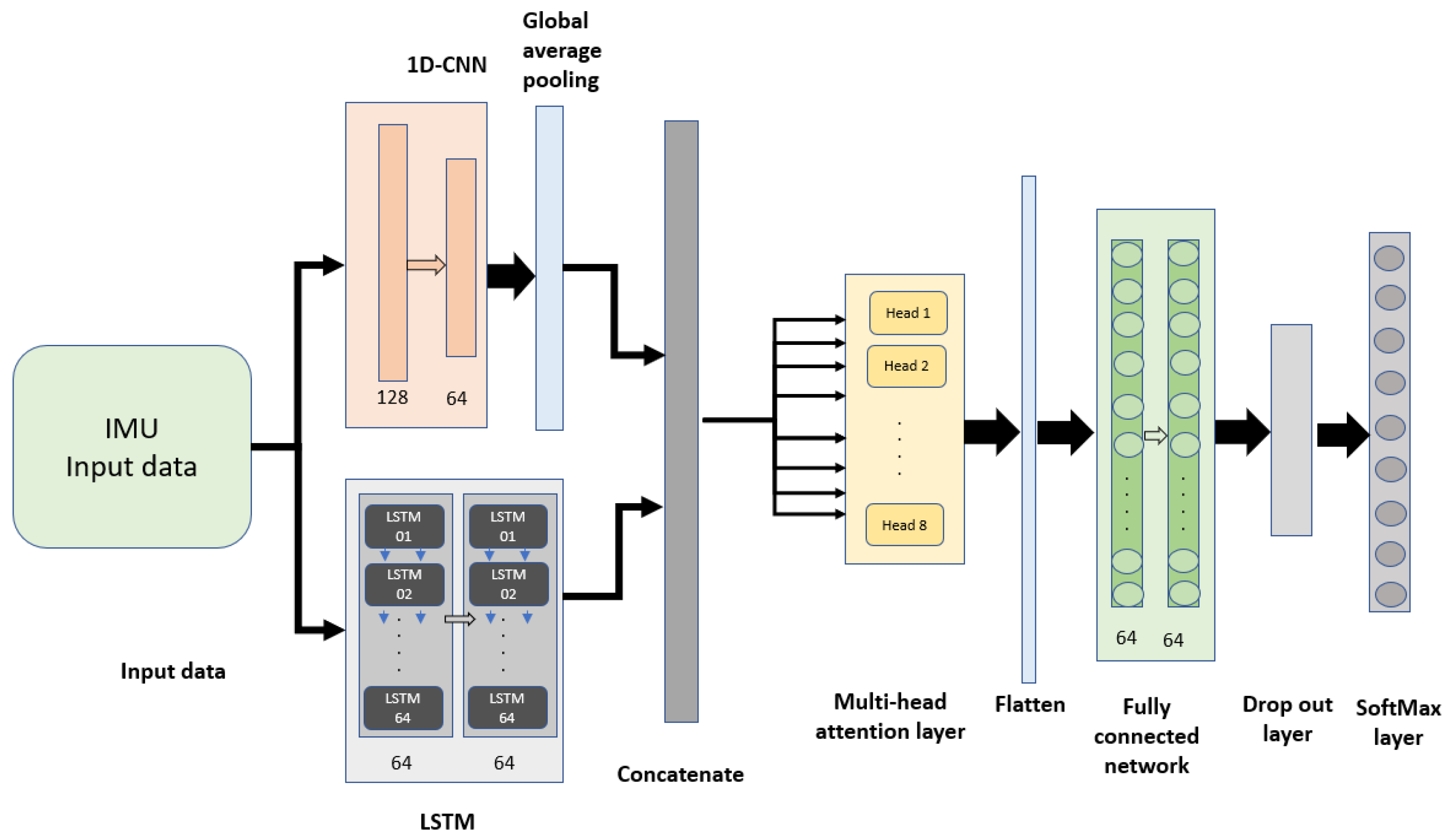
3.2.2. Parallel Feature Fusion Model

In the parallel fusion model, the input data from the sensor is simultaneously fed into both the CNN and LSTM networks as shown in Figure 4. The output from the CNN is processed by a global average pooling layer, which averages the time-series data, while the LSTM outputs the data from the last time step. The output features from both the CNN and LSTM networks were concatenated to form a unified feature vector. This vector was then passed through an eight-head multi-head attention mechanism. In the final stage, a dense network with two layers, followed by a dropout layer and a softmax function, was used for classification. The primary distinction between the cascaded model and the parallel model lies in how the features from the CNN and LSTM networks are fused. In the cascaded model, the features are passed sequentially from the CNN to the LSTM, while in the parallel model, the features are extracted from both networks simultaneously and then combined.

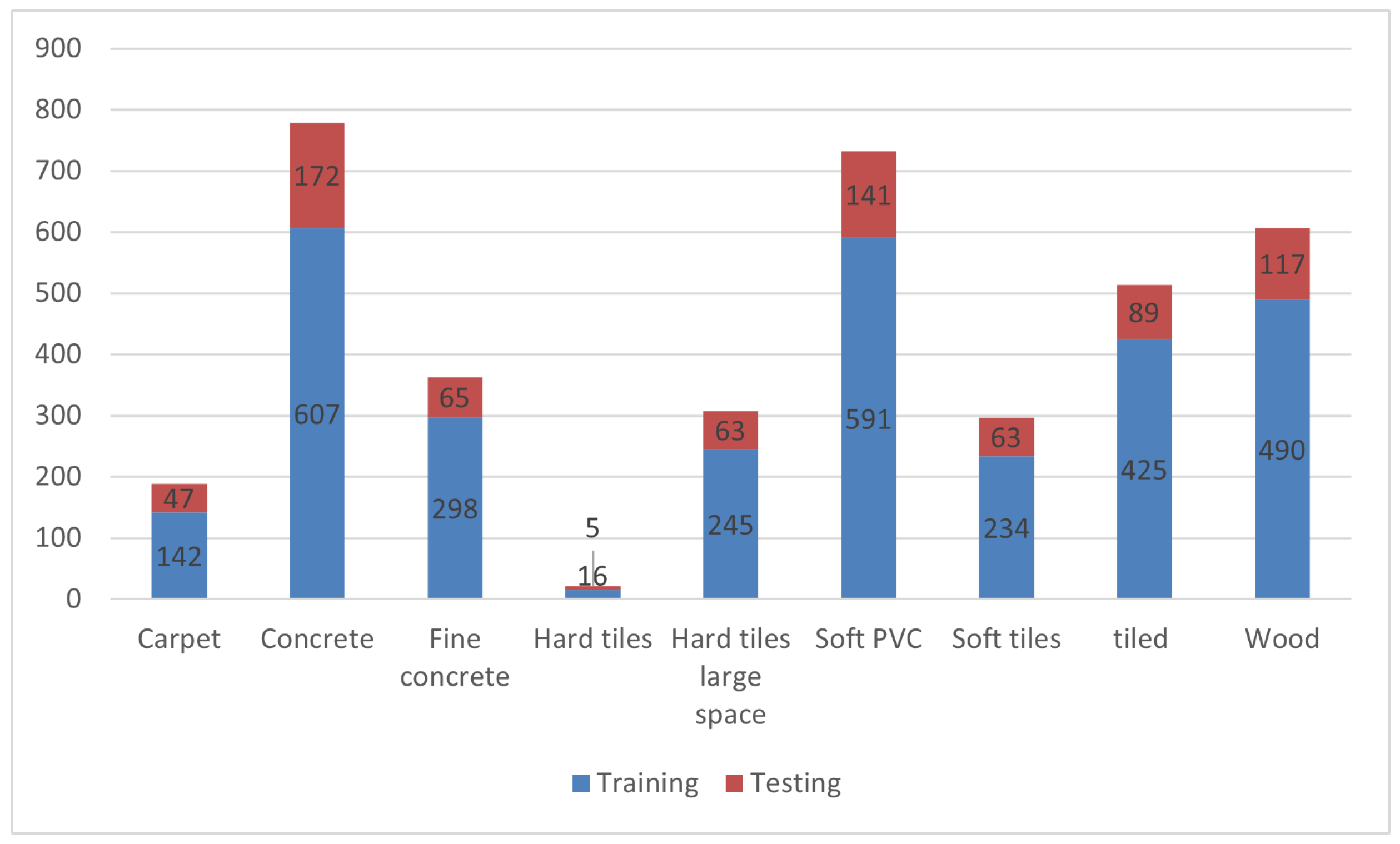
4. Dataset and Training Process

The time-series dataset analyzed in this study is collected from an IMU sensor mounted on a ground robot [46]. The IMU used for data collection is the XSENS MTi-300, a sensor manufactured by Movella, a company based in Henderson, NV, USA [47]. The sensor operates at a frequency of 375 Hz, resulting in 0.341 s per sequence (128 data point). The dataset comprises ten features representing a four-dimensional quaternion space: x orientation, y orientation, z orientation, and the angle of rotation. Additionally, it includes the three angular velocities and the three linear accelerations in the x, y, and z directions. The robot was driven over nine different surface types, and the data were annotated into nine classes: hard tiles with large spaces, hard tiles, soft tiles, fine concrete, concrete, soft PVC, tiles, and wood. The dataset is publicly available on Kaggle [48].

The data were normalized by subtracting the mean and dividing by the standard deviation to ensure all features were on a consistent scale. The dataset includes 3810 annotated time sequences, where each sequence consists of 128 data points. The dataset was divided into training and testing sets, with 80% allocated for training and 20% for testing. This resulted in 3048 training points and 762 testing points. The majority of the dataset is used for training so the models can learn patterns effectively. More training data help improve generalization and prevent underfitting. Figure 5 shows the histogram of the dataset annotations and the distribution of training and testing among each class.

The training process was applied to both models, the cascaded feature fusion and the parallel feature fusion, using cross-validation. The training data were divided into five groups, with four groups used for training and one for validation. In each epoch, the validation set changes, ensuring that the models are trained on the entire training set across all iterations. A grid search was implemented during training to find the best hyperparameters for the models. The hyperparameters considered in the grid search included epoch count, batch size, optimizer choice, dropout rate, number of attention heads, and the key vector dimension. The optimal hyperparameters identified through this grid search are summarized in

Table 1. The hyperparameters of the models based on the grid search.

Hyperparameter	Value
Batch size	32
Epoch size	60
Optimization function	Adam
dropout rate	0.2
Attention mechanism number of heads	8
Attention mechanism key vector dimension	64
Number of LSTM units	64

. The model was compiled using the Adam optimizer with the default learning rate of 0.001. No learning rate scheduling was applied during training. The cross-validation score for the cascaded feature fusion model is 0.753, while the parallel feature fusion model achieved a cross-validation of 0.77. The models are trained and tested using a computer with 12th Gen Intel Core i7-1.70 GHz, manufactured by Intel company that is located on Santa Clara, CA, USA, with RAM of 8 GB.

5. Evaluation Metrics

To evaluate the proposed models, the LSTM model was used as a baseline for comparison. Additionally, the cascaded fusion model and the parallel fusion model were assessed both against the baseline and in comparison to each other. The classification performance was quantified using precision, recall, F1 score, and Mean Average Precision (mAP), as defined in [49]. Precision, which measures the proportion of correctly identified positive cases among all predicted positives, is defined in Equation (3):

$$Precision={\displaystyle \frac{1}{N}}\sum _{i=1}^N{\displaystyle \frac{TP}{TP+FP}}$$

(3)

Recall, indicating the proportion of correctly identified positive cases out of all actual positives, is defined in Equation (4):

$$Recall={\displaystyle \frac{1}{N}}\sum _{i=1}^N{\displaystyle \frac{TP}{TP+FN}}$$

(4)

Here, TP refers to true positive, TN to true negative, FP to false positives and FN is to false negatives.

The F1 score, a harmonic mean of precision and recall, is expressed in Equation (5):

$$F1=2\times {\displaystyle \frac{Precision\times Recall}{Precision+Recall}}$$

(5)

Finally, the mean Average Precision (mAP), representing the average of the individual Average Precision (AP) values across all classes, is computed, as shown in Equation (6):

$$\mathrm{mAP}={\displaystyle \frac{1}{N}}\sum _{i=1}^N{\mathrm{AP}}_i$$

(6)

where N is the number of classes, and ${\mathrm{AP}}_i$ is the Average Precision for class i.

6. Results

6.1. Baseline vs. Cascaded Fusion Model

Table 2. Comparison of Baseline (LSTM) and the cascaded fusion model.

Metric	Baseline (LSTM)	Cascaded (CNN-LSTM)	Cascaded (CNN-LSTM + Attention)	% Improvement (Cascaded Model to LSTM)
Precision	0.764	0.787	0.835	+9.3%
Recall	0.752	0.777	0.833	+10.8%
F1 Score	0.751	0.779	0.833	+10.9%
mAP	0.608	0.647	0.721	+18.6%
Runtime (ms)	580	590	1420	−144.8%

presents a comparative analysis of the classification results and runtime of the cascaded fusion model relative to the LSTM baseline. The results reveal a substantial improvement in classification accuracy, with the mAP increasing by 18.8%. However, this enhancement in performance was accompanied by a notable increase in runtime, which rose from 580 ms for the LSTM model to 1420 ms for the cascaded fusion model, representing a 144.8% increase. It is important to note that in the improvement column of the table, a negative value signifies a reduction in performance.

6.2. Baseline vs. Parallel Fusion Model

Table 3. Comparison of Baseline (LSTM) and parallel fusion Models.

Metric	Baseline (LSTM)	Parallel (CNN-LSTM)	Parallel (CNN-LSTM + Attention)	% Improvement (Parallel Model to LSTM)
Precision	0.764	0.794	0.815	+6.7%
Recall	0.752	0.793	0.813	+8.1%
F1 Score	0.751	0.791	0.813	+8.3%
mAP	0.608	0.662	0.693	+14.0%
Runtime (ms)	580	580	630	−8.6%

provides a comparative analysis of the parallel fusion model and the baseline algorithm. The results indicate a significant enhancement in detection accuracy, with the mAP increasing by 14%. Collectively. It also shows an increment in the runtime by 50 ms (8.6%) compared to the baseline.

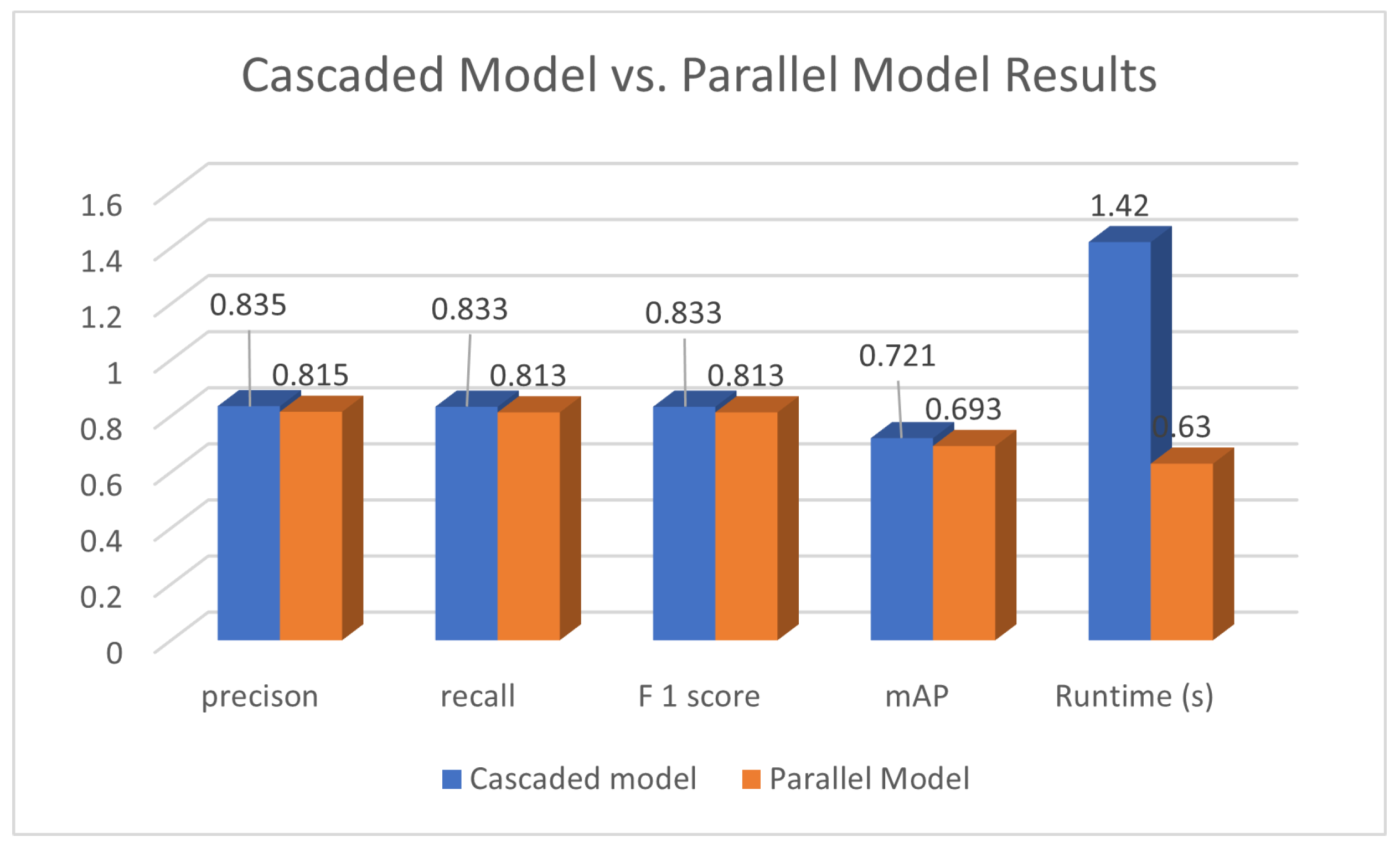
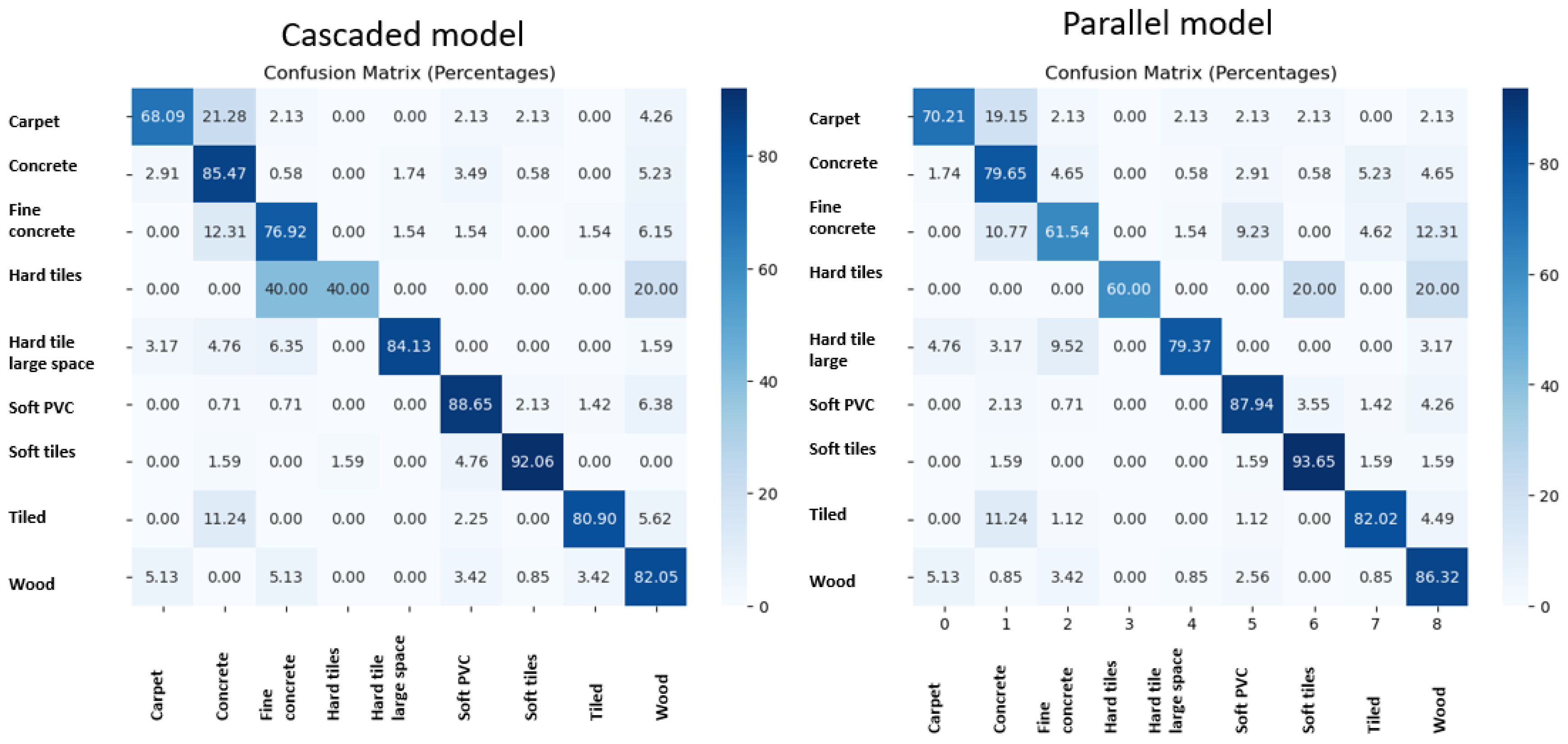
6.3. Cascaded Fusion Model vs. Parallel Fusion Model

Table 4. Comparison of the cascaded fusion model and parallel fusion model.

Metric	Cascaded (CNN-LSTM + Attention)	Parallel (CNN-LSTM + Attention)	% Improvement (Cascaded to Parallel Fusion Model)
Precision	0.835	0.815	+2.4%
Recall	0.833	0.813	+2.4%
F1 Score	0.833	0.813	+2.4%
mAP	0.721	0.693	+3.9%
Runtime (ms)	1420	630	−55.6%

presents a detailed comparison of parallel and cascaded feature fusion models. The cascaded model demonstrates superior performance across all metrics, particularly in mAP (0.721 vs. 0.693), achieving precision, recall, and F1-score of 0.835, 0.833, and 0.833, respectively. While offering superior classification accuracy, the cascaded model incurs a significant computational cost, requiring 1420 ms per evaluation, compared to 630 ms for the parallel model, representing a 55.6% increase in processing time.

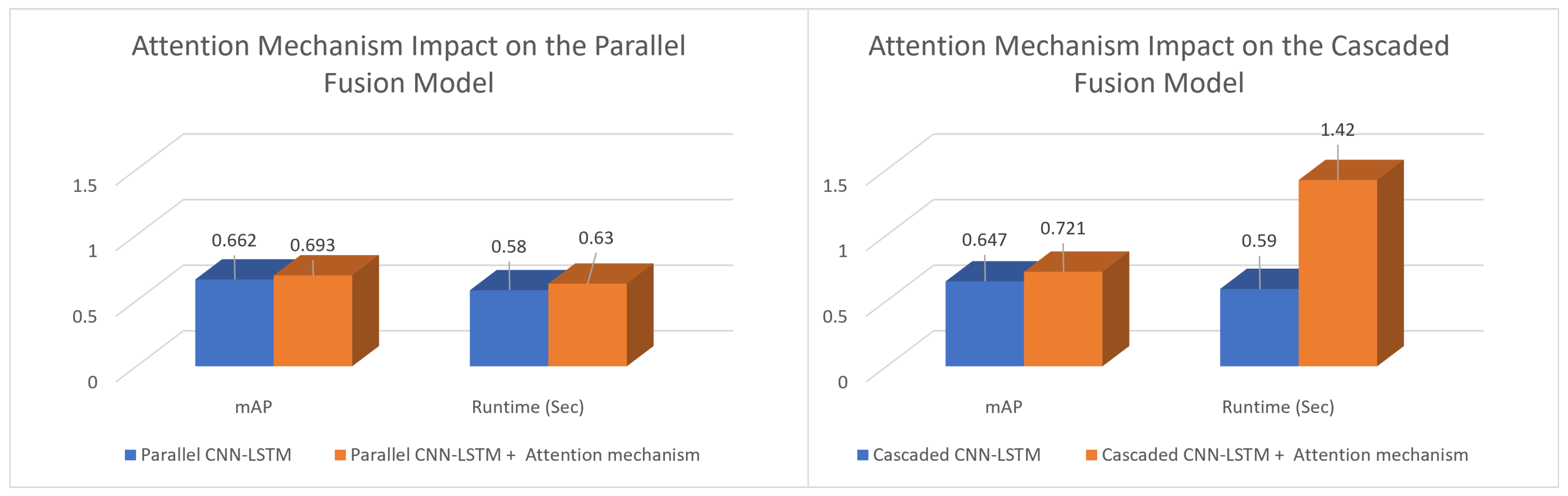
6.4. The Multi-Head Attention Mechanism Impact

Figure 6 illustrates the impact of the multi-head attention mechanism on the performance of both fusion models. In the parallel fusion architecture, the incorporation of attention resulted in a modest increase in mAP from 0.662 to 0.693, accompanied by a 50 ms increase in runtime. Conversely, the cascaded fusion model exhibited a more substantial improvement, with mAP rising from 0.647 to 0.721, representing a 14% enhancement in accuracy. However, this significant accuracy gain came at a substantial computational cost, as the processing time increased significantly from 590 ms to 1420 ms. These results underscore the inherent trade-off between accuracy and computational efficiency when utilizing the multi-head attention mechanism within the proposed surface classification framework.

The multi-head attention mechanism is likely more effective in the cascaded model because it can focus on the most relevant features at each step in the sequence, enabling the model to better capture long-range dependencies in the data. In the parallel model, while multi-head attention still improves performance by weighting the contributions of each branch, the independent processing of data streams limits the attention’s ability to significantly influence the interaction between the CNN and LSTM features.

7. Discussion

Comparative analysis of cascaded and parallel fusion models highlights critical trade-offs between detection accuracy and computational efficiency. As depicted in Figure 7, the cascaded fusion model achieved marginally higher precision, recall, and mAP scores, indicating superior detection accuracy. In contrast, the parallel fusion model excelled in classification runtime, positioning it as a more computationally efficient and well-balanced alternative. The parallel model provides an effective balance between delivering satisfactory detection performance and minimizing computational overhead.

The significance of each component within the proposed models is highlighted by assessing its individual performance apart from other elements. For instance, the LSTM alone achieved an mAP of 0.608, which rose to 0.647 with the cascaded fusion of CNN and LSTM features, and further to 0.662 with the parallel fusion of CNN and LSTM. The addition of the multi-head attention mechanism proved more impact in the cascaded fusion model, boosting mAP by 11.44%, as compared to a 4.23% increase observed in the parallel fusion model. However, adding the multi-head attention module in the cascaded fusion model increased the processing time from 0.59 s to 1.42 s.

Figure 8 displays the confusion matrix for both the cascaded fusion model and the parallel fusion model. It is evident that the cascaded fusion model achieved higher true-positive rates across most classes compared to the parallel fusion model. For example, the cascade model exhibited true-positive rates of 85.47% for concrete and 76.92% for fine concrete, while the parallel fusion model recorded true positives of 79.65% and 61.54% respectively. The parallel model demonstrated significant improvements in specific classes; for instance, the false-positive rate for classifying hard tiles as fine concrete was reduced from 40% in the cascaded fusion model to 0% in the parallel fusion model. The parallel model demonstrated better performance in classes with similarities, such as concrete and fine concrete.

8. Conclusions

This study investigates surface type classification using Inertial Measurement Unit (IMU) data acquired from a ground robot. Two novel feature fusion architectures are proposed and evaluated. The cascaded model employs a sequential feature extraction approach, integrating a 1-D Convolutional Neural Network (CNN) followed by a Long Short-Term Memory (LSTM) network. Alternatively, the parallel fusion model leverages parallel processing, where the IMU data are concurrently processed by both 1-D CNN and LSTM networks, and the resulting feature representations are subsequently concatenated. To enhance the model’s ability to focus on the most relevant information within the sensor data, a multi-head attention mechanism is incorporated into both architectures.

The proposed models were trained and evaluated on a time series dataset. Data normalization, employing a standard z-score transformation (subtracting the mean and dividing by the standard deviation), enhanced the detection performance of both models. Hyperparameter optimization was performed using a grid search approach to ensure optimal model performance. Experimental results demonstrated that the cascaded fusion model achieved marginally superior detection metrics, including precision, mean Average Precision (mAP), recall, and F1-score, compared to the parallel fusion model. This suggests that the cascaded approach enables better feature representation and extraction, leading to more accurate detections. However, the cascaded fusion system exhibited a significantly higher computational cost, with a 55.6% increase in processing time. The integration of the multi-head attention mechanism significantly contributed to improved detection accuracy, particularly within the cascaded feature fusion model, though at the expense of increased classification runtime. In conclusion, the parallel fusion model offers a more optimized solution, effectively balancing detection accuracy and computational efficiency.

Future research directions could involve a comparative analysis between IMU-based deep learning and computer vision systems. By integrating both systems onto a single robotic platform, a comprehensive evaluation of detection accuracy and runtime performance could be conducted. Furthermore, exploring the synergistic potential of fusing IMU data with visual sensor inputs holds significant promise for enhancing surface classification capabilities.

References

1. Wang, H.; Luo, N.; Zhou, T.; Yang, S. Physical Robots in Education: A Systematic Review Based on the Technological Pedagogical Content Knowledge Framework. Sustainability 2024, 16, 4987. [Google Scholar] [CrossRef]
2. Obrenovic, B.; Gu, X.; Wang, G.; Godinic, D.; Jakhongirov, I. Generative AI and human–robot interaction: Implications and future agenda for business, society and ethics. AI Soc. 2024, 1–14. [Google Scholar] [CrossRef]
3. Silvera-Tawil, D. Robotics in Healthcare: A Survey. SN Comput. Sci. 2024, 5, 189. [Google Scholar]
4. Walas, K. Terrain classification and negotiation with a walking robot. J. Intell. Robot. Syst. 2015, 78, 401–423. [Google Scholar]
5. Khaleghian, S.; Taheri, S. Terrain classification using intelligent tire. J. Terramech. 2017, 71, 15–24. [Google Scholar]
6. Oliveira, F.G.; Santos, E.R.; Neto, A.A.; Campos, M.F.; Macharet, D.G. Speed-invariant terrain roughness classification and control based on inertial sensors. In Proceedings of the 2017 Latin American Robotics Symposium (LARS) and 2017 Brazilian Symposium on Robotics (SBR), São Paulo, Brazil, 19–21 October 2017; pp. 1–6. [Google Scholar]
7. Hoepflinger, M.A.; Remy, C.D.; Hutter, M.; Spinello, L.; Siegwart, R. Haptic terrain classification for legged robots. In Proceedings of the 2010 IEEE International Conference on Robotics and Automation, Anchorage, AK, USA, 3–7 May 2010; pp. 2828–2833. [Google Scholar]
8. Zenker, S.; Aksoy, E.E.; Goldschmidt, D.; Wörgötter, F.; Manoonpong, P. Visual terrain classification for selecting energy efficient gaits of a hexapod robot. In Proceedings of the 2013 IEEE/ASME International Conference on Advanced Intelligent Mechatronics, Wollongong, NSW, Australia, 9–12 July 2013; pp. 577–584. [Google Scholar]
9. Zhao, T.; Guo, P.; Wei, Y. Road friction estimation based on vision for safe autonomous driving. Mech. Syst. Signal Process. 2024, 208, 111019. [Google Scholar]
10. Iglesias, F.; Aguilera, A.; Padilla, A.; Vizán, A.; Diez, E. Application of computer vision techniques to estimate surface roughness on wood-based sanded workpieces. Measurement 2024, 224, 113917. [Google Scholar]
11. Laible, S.; Khan, Y.N.; Zell, A. Terrain classification with conditional random fields on fused 3D LIDAR and camera data. In Proceedings of the 2013 European Conference on Mobile Robots, Warsaw, Poland, 2–4 September 2013; pp. 172–177. [Google Scholar]
12. Walas, K.; Nowicki, M. Terrain classification using laser range finder. In Proceedings of the 2014 IEEE/RSJ International Conference on Intelligent Robots and Systems, Chicago, IL, USA, 14–18 September 2014; pp. 5003–5009. [Google Scholar]
13. Borrmann, D.; Nüchter, A.; Ðakulović, M.; Maurović, I.; Petrović, I.; Osmanković, D.; Velagić, J. A mobile robot based system for fully automated thermal 3D mapping. Adv. Eng. Inform. 2014, 28, 425–440. [Google Scholar] [CrossRef]
14. Hu, K.; Chen, Z.; Kang, H.; Tang, Y. 3D vision technologies for a self-developed structural external crack damage recognition robot. Autom. Constr. 2024, 159, 105262. [Google Scholar]
15. Tang, Y.; Huang, Z.; Chen, Z.; Chen, M.; Zhou, H.; Zhang, H.; Sun, J. Novel visual crack width measurement based on backbone double-scale features for improved detection automation. Eng. Struct. 2023, 274, 115158. [Google Scholar]
16. Yi, J.; Zhang, J.; Song, D.; Jayasuriya, S. IMU-based localization and slip estimation for skid-steered mobile robots. In Proceedings of the 2007 IEEE/RSJ International Conference on Intelligent Robots and Systems, San Diego, CA, USA, 29 October–2 November 2007; pp. 2845–2850. [Google Scholar]
17. Botero Valencia, J.S.; Rico Garcia, M.; Villegas Ceballos, J.P. A simple method to estimate the trajectory of a low cost mobile robotic platform using an IMU. Int. J. Interact. Des. Manuf. (IJIDeM) 2017, 11, 823–828. [Google Scholar]
18. Apaydın, N.N.; Kılıç, İ.; Apaydın, M.; Yaman, O. Decision Tree-Based Direction Detection Using IMU Data in Autonomous Robots. Batman Üniv. Yaşam Bilim. Derg. 2024, 14, 57–68. [Google Scholar]
19. Zevering, J.; Bredenbeck, A.; Arzberger, F.; Borrmann, D.; Nüchter, A. IMU-based pose-estimation for spherical robots with limited resources. In Proceedings of the 2021 IEEE International Conference on Multisensor Fusion and Integration for Intelligent Systems (MFI), Seoul, Republic of Korea, 25–27 August 2021; pp. 1–8. [Google Scholar]
20. Barnea, A.; Berrabah, S.A.; Oprisan, C.; Doroftei, I. IMU (Inertial Measurement Unit) Integration for the Navigation and Positioning of Autonomous Robot Systems. J. Control. Eng. Appl. Inform. 2011, 13, 38–43. [Google Scholar]
21. Wang, L.; Jiang, Z.; Hu, Y.; Yang, S. Research on the Self-Stability Control and Gait Planning of Quadruped Robot Based on IMU. In Proceedings of the 2021 IEEE 21st International Conference on Communication Technology (ICCT), Xi’an, China, 19–21 October 2021; pp. 1078–1081. [Google Scholar]
22. Hammoudeh, M.A.A.; Alsaykhan, M.; Alsalameh, R.; Althwaibi, N. Computer Vision: A Review of Detecting Objects in Videos–Challenges and Techniques. Int. J. Online Biomed. Eng. 2022, 18, 15. [Google Scholar]
23. Mariniello, G.; Pastore, T.; Menna, C.; Festa, P.; Asprone, D. Structural damage detection and localization using decision tree ensemble and vibration data. Comput. Aided Civ. Infrastruct. Eng. 2021, 36, 1129–1149. [Google Scholar]
24. Kumar, P.; Pandi, S.S.; Kumaragurubaran, T.; Chiranjeevi, V.R. Human Activity Recognitions in Handheld Devices Using Random Forest Algorithm. In Proceedings of the 2024 International Conference on Automation and Computation (AUTOCOM), Dehradun, India, 14–16 March 2024; pp. 159–163. [Google Scholar]
25. Al-refai, G.; Elmoaqet, H.; Ryalat, M. In-vehicle data for predicting road conditions and driving style using machine learning. Appl. Sci. 2022, 12, 8928. [Google Scholar] [CrossRef]
26. Barman, U.; Choudhury, R.D. Soil texture classification using multi class support vector machine. Inf. Process. Agric. 2020, 7, 318–332. [Google Scholar]
27. Kim, D.; Kim, S.H.; Kim, T.; Kang, B.B.; Lee, M.; Park, W.; Ku, S.; Kim, D.; Kwon, J.; Lee, H.; et al. Review of machine learning methods in soft robotics. PLoS ONE 2021, 16, e0246102. [Google Scholar]
28. Shirmard, H.; Farahbakhsh, E.; Müller, R.D.; Chandra, R. A review of machine learning in processing remote sensing data for mineral exploration. Remote Sens. Environ. 2022, 268, 112750. [Google Scholar]
29. Gupta, S. Deep learning based human activity recognition (HAR) using wearable sensor data. Int. J. Inf. Manag. Data Insights 2021, 1, 100046. [Google Scholar]
30. Qi, W.; Ovur, S.E.; Li, Z.; Marzullo, A.; Song, R. Multi-sensor guided hand gesture recognition for a teleoperated robot using a recurrent neural network. IEEE Robot. Autom. Lett. 2021, 6, 6039–6045. [Google Scholar] [CrossRef]
31. Zhu, J.; Chen, H.; Ye, W. Classification of human activities based on radar signals using 1D-CNN and LSTM. In Proceedings of the 2020 IEEE International Symposium on Circuits and Systems (ISCAS), Seoul, Republic of Korea, 18–22 October 2020; pp. 1–5. [Google Scholar]
32. Al-refai, G.; Al-refai, M.; Alzu’bi, A. Driving Style and Traffic Prediction with Artificial Neural Networks Using On-Board Diagnostics and Smartphone Sensors. Appl. Sci. 2024, 14, 5008. [Google Scholar] [CrossRef]
33. Mekruksavanich, S.; Jitpattanakul, A. Lstm networks using smartphone data for sensor-based human activity recognition in smart homes. Sensors 2021, 21, 1636. [Google Scholar] [CrossRef] [PubMed]
34. Pham, T.D. Time–frequency time–space LSTM for robust classification of physiological signals. Sci. Rep. 2021, 11, 6936. [Google Scholar]
35. Matar, M.; Xia, T.; Huguenard, K.; Huston, D.; Wshah, S. Multi-head attention based bi-lstm for anomaly detection in multivariate time-series of wsn. In Proceedings of the 2023 IEEE 5th International Conference on Artificial Intelligence Circuits and Systems (AICAS), Bangalore, India, 9–11 March 2023; pp. 1–5. [Google Scholar]
36. Junior, R.F.R.; dos Santos Areias, I.A.; Campos, M.M.; Teixeira, C.E.; da Silva, L.E.B.; Gomes, G.F. Fault detection and diagnosis in electric motors using 1d convolutional neural networks with multi-channel vibration signals. Measurement 2022, 190, 110759. [Google Scholar]
37. Cui, W.; Deng, X.; Zhang, Z. Improved convolutional neural network based on multi-head attention mechanism for industrial process fault classification. In Proceedings of the 2020 IEEE 9th Data Driven Control and Learning Systems Conference (DDCLS), Hangzhou, China, 23–25 October 2020; pp. 918–922. [Google Scholar]
38. Li, X.; Wu, J.; Li, Z.; Zuo, J.; Wang, P. Robot ground classification and recognition based on CNN-LSTM model. In Proceedings of the 2021 IEEE 2nd International Conference on Big Data, Artificial Intelligence and Internet of Things Engineering (ICBAIE), Beijing, China, 16–18 December 2021; pp. 1110–1113. [Google Scholar]
39. AlRadaideh, S.; Aljoan, I.; Al-refai, G.; Elmoaqet, H. Ground Classification for Robots Navigation Using Time Series Dataset with LSTM and CNN. In Proceedings of the 2024 22nd International Conference on Research and Education in Mechatronics (REM), Dead Sea, Jordan, 24–26 September 2024; pp. 375–380. [Google Scholar]
40. Feng, C.; Dong, K.; Ou, X. A Robot Ground Medium Classification Algorithm Based on Feature Fusion and Adaptive Spatio-Temporal Cascade Networks. Neural Process. Lett. 2024, 56, 235. [Google Scholar]
41. Jiang, Y.; Zhou, W.; Zhang, S.; Gao, S. Floor Surface Classification with Robot IMU Sensors Data. Available online: https://noiselab.ucsd.edu/ECE228_2019/Reports/Report14.pdf (accessed on 17 March 2025).
42. Kiranyaz, S.; Avci, O.; Abdeljaber, O.; Ince, T.; Gabbouj, M.; Inman, D.J. 1D convolutional neural networks and applications: A survey. Mech. Syst. Signal Process. 2021, 151, 107398. [Google Scholar] [CrossRef]
43. Van Houdt, G.; Mosquera, C.; Nápoles, G. A review on the long short-term memory model. Artif. Intell. Rev. 2020, 53, 5929–5955. [Google Scholar]
44. Hanin, B. Which neural net architectures give rise to exploding and vanishing gradients? Adv. Neural Inf. Process. Syst. 2018, 31, 580–589. [Google Scholar]
45. Niu, Z.; Zhong, G.; Yu, H. A review on the attention mechanism of deep learning. Neurocomputing 2021, 452, 48–62. [Google Scholar]
46. Lomio, F.; Skenderi, E.; Mohamadi, D.; Collin, J.; Ghabcheloo, R.; Huttunen, H. Surface type classification for autonomous robot indoor navigation. arXiv 2019, arXiv:1905.00252. [Google Scholar]
47. Movella. Datasheet for XSENS MTi-300 IMU. Available online: https://www.xsens.com/hubfs/Downloads/Leaflets/MTi-300.pdf (accessed on 17 March 2025).
48. Maggie; Dane, S. CareerCon 2019—Help Navigate Robots. Available online: https://kaggle.com/competitions/career-con-2019 (accessed on 19 October 2024).
49. Erickson, B.J.; Kitamura, F. Magician’s Corner: 9. Performance Metrics for Machine Learning Models. Radiol. Artif. Intell. 2021, 3, e200126. [Google Scholar] [CrossRef]
Figure 1. Architecture of Long-Short Term Memory (LSTM) unit [43].
Machines 13 00251 g001
Figure 3. The cascaded CNN-LSTM with multi-head attention system for surface classification.
Machines 13 00251 g003
Figure 4. The parallel CNN-LSTM with multi-head attention system for surface classification.
Machines 13 00251 g004
Figure 5. The dataset count and the number of training and testing points for each class.
Machines 13 00251 g005
Figure 6. Histogram illustrating the impact of the multi-head attention mechanism on the parallel and cascaded fusion models, comparing mAP and runtime.
Machines 13 00251 g006
Figure 7. Histogram representation of the parallel model vs. the cascaded model classification results and runtime.
Machines 13 00251 g007
Figure 8. Confusion matrix of the casaded fusion model and parallel fusion model.
Machines 13 00251 g008