
Comparison of Induction Machine Drive Control Schemes on the Distribution of Power Losses in a Three-Level NPC Converter


Abstract
1. Introduction
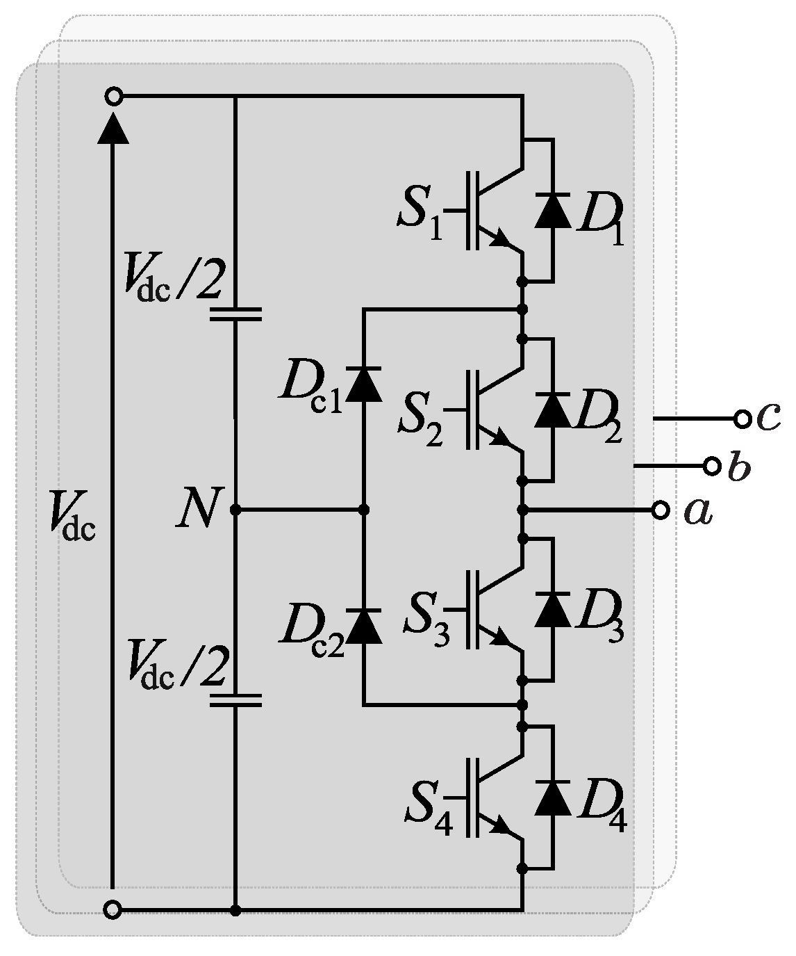
2. Converter Topology
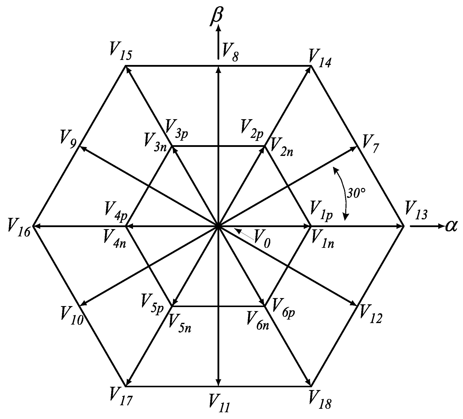
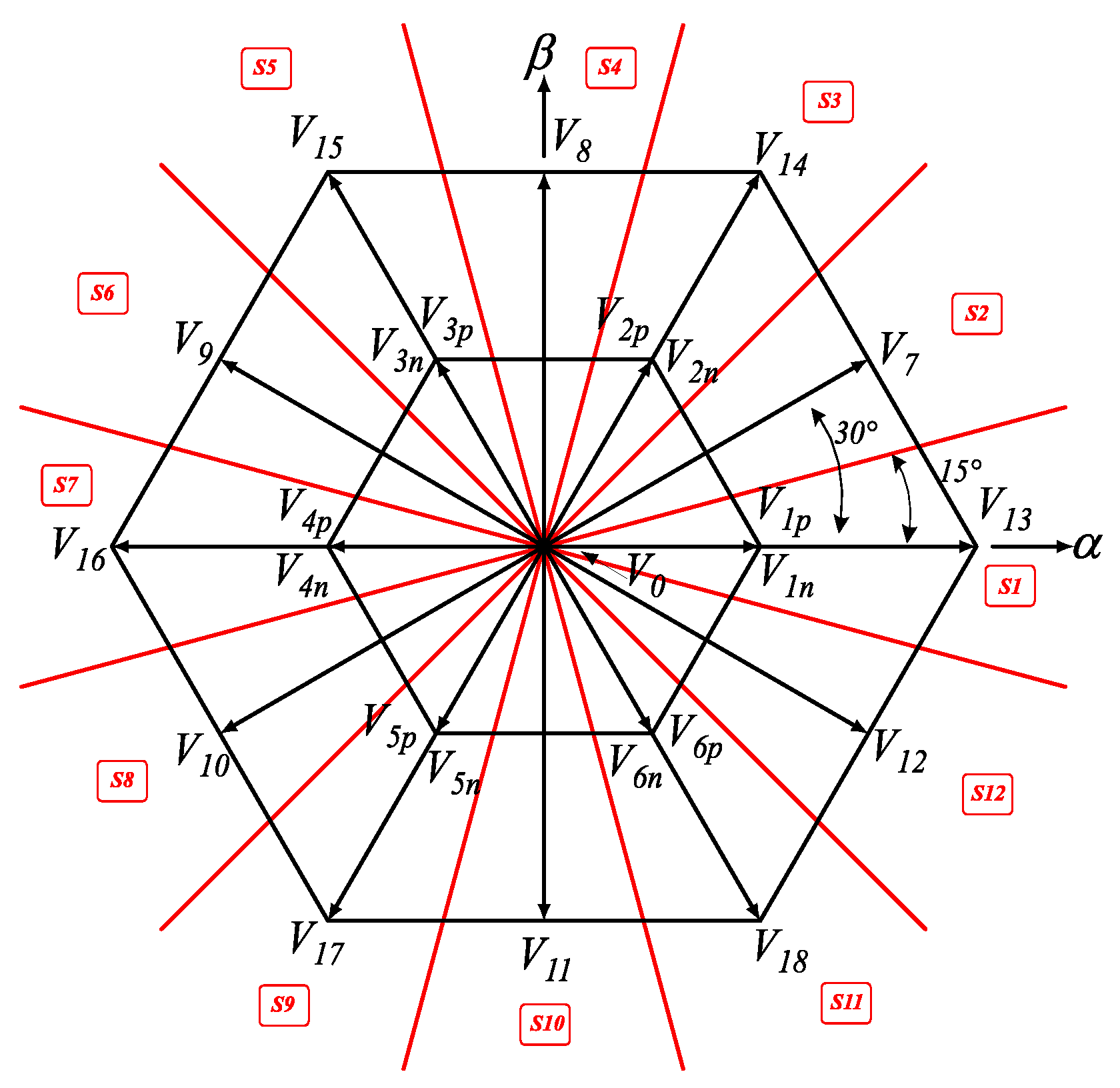
- Zero vector (): 3 redundancies with magnitude 0.
- Small vector (): 2 redundancies with magnitude
- Medium vector (): no redundancies with magnitude equal to
- Large vector (): no redundancies with magnitude equal to
3. Semiconductor Thermal Model
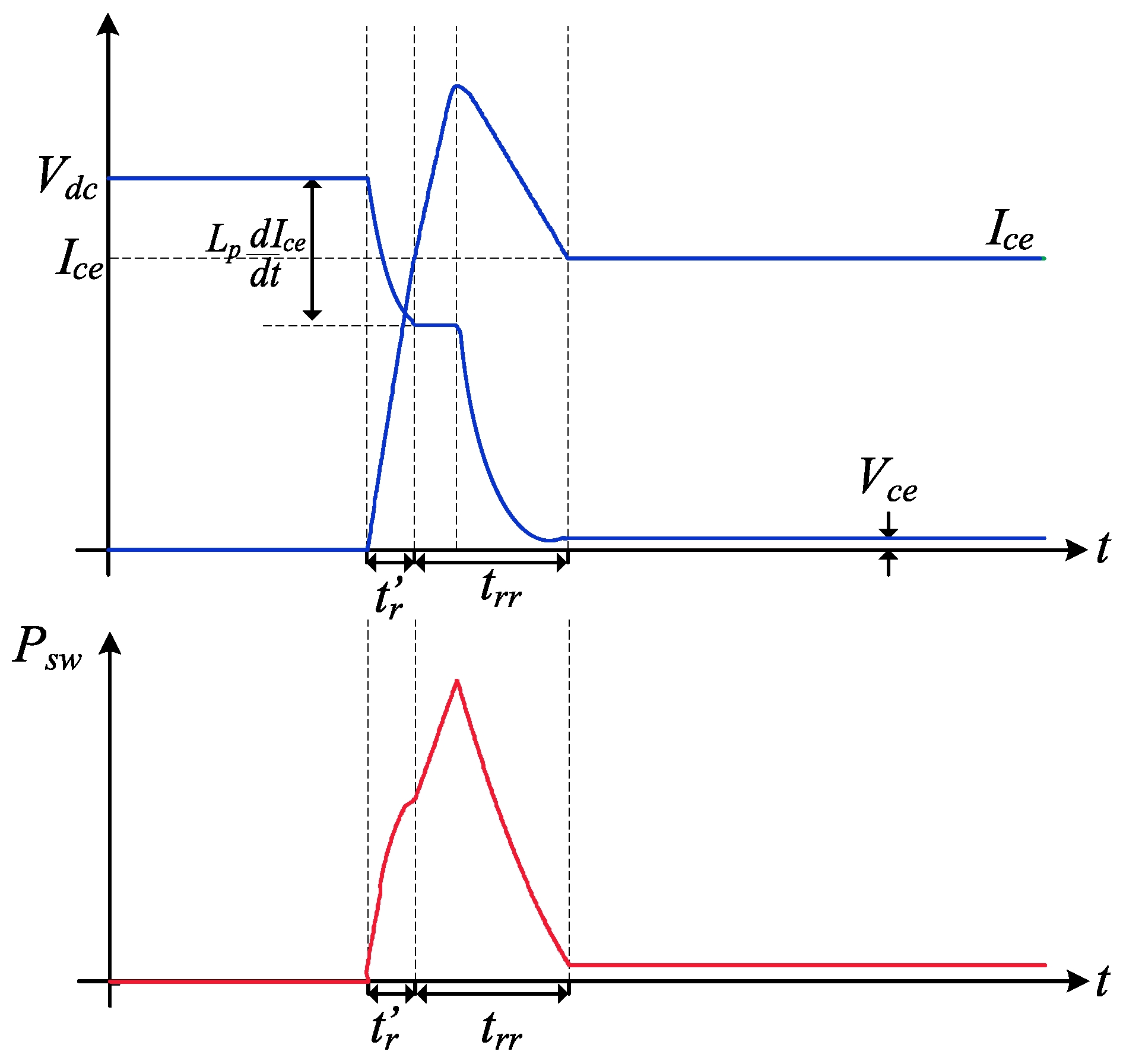
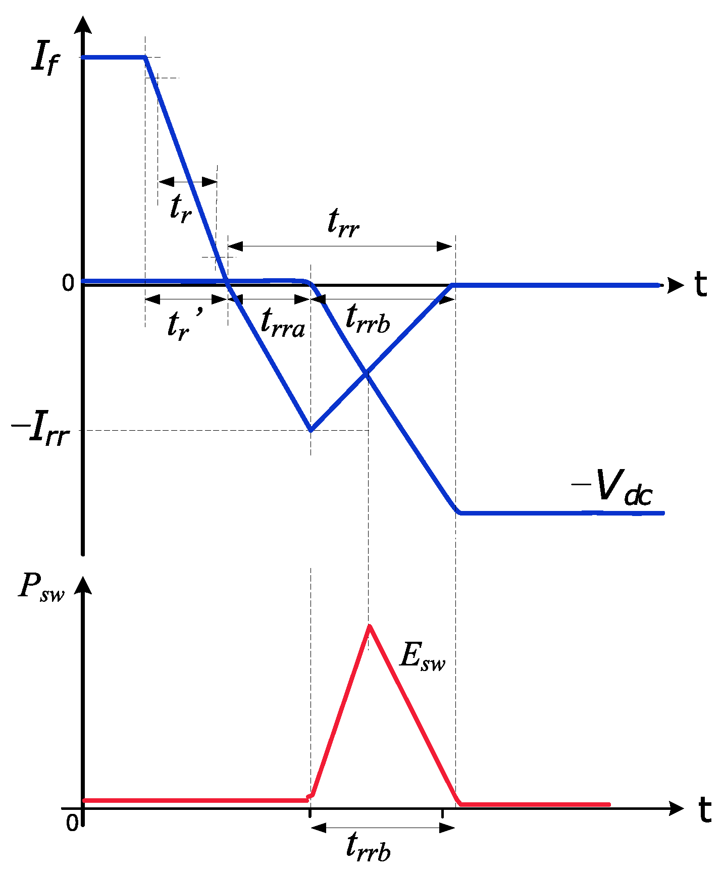
- Reverse recovery time;
- Rise and fall operating characteristics;
- Operating temperature.
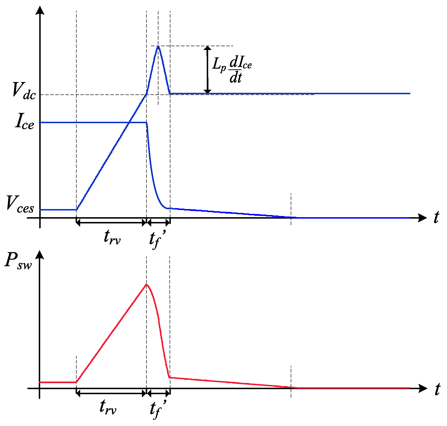
3.1. Conduction and Switching Losses Mechanism
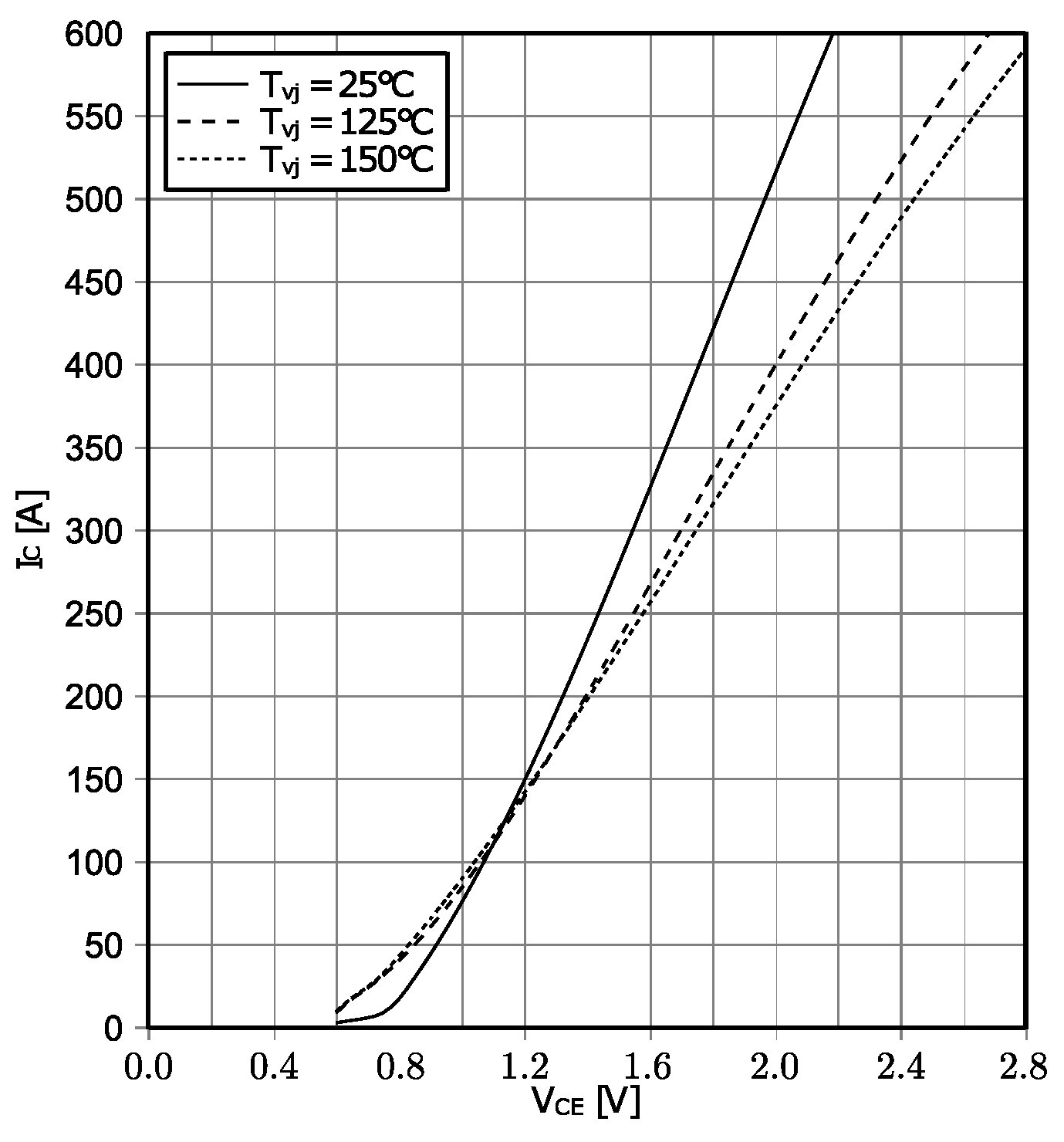
3.2. Conduction Loss Calculation
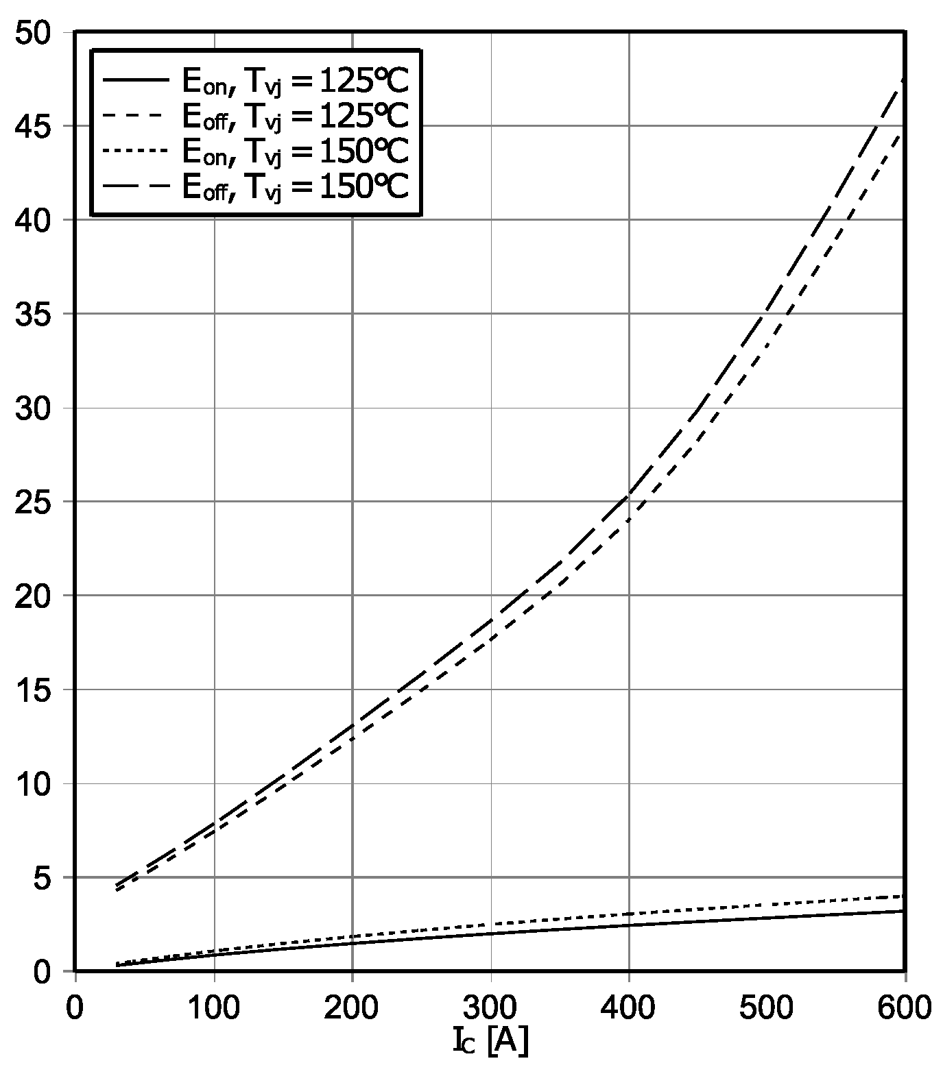
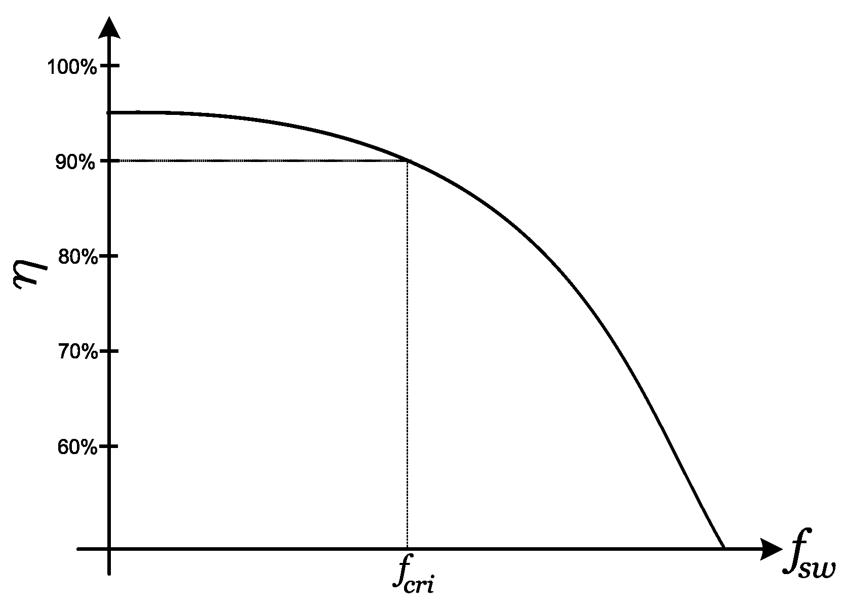
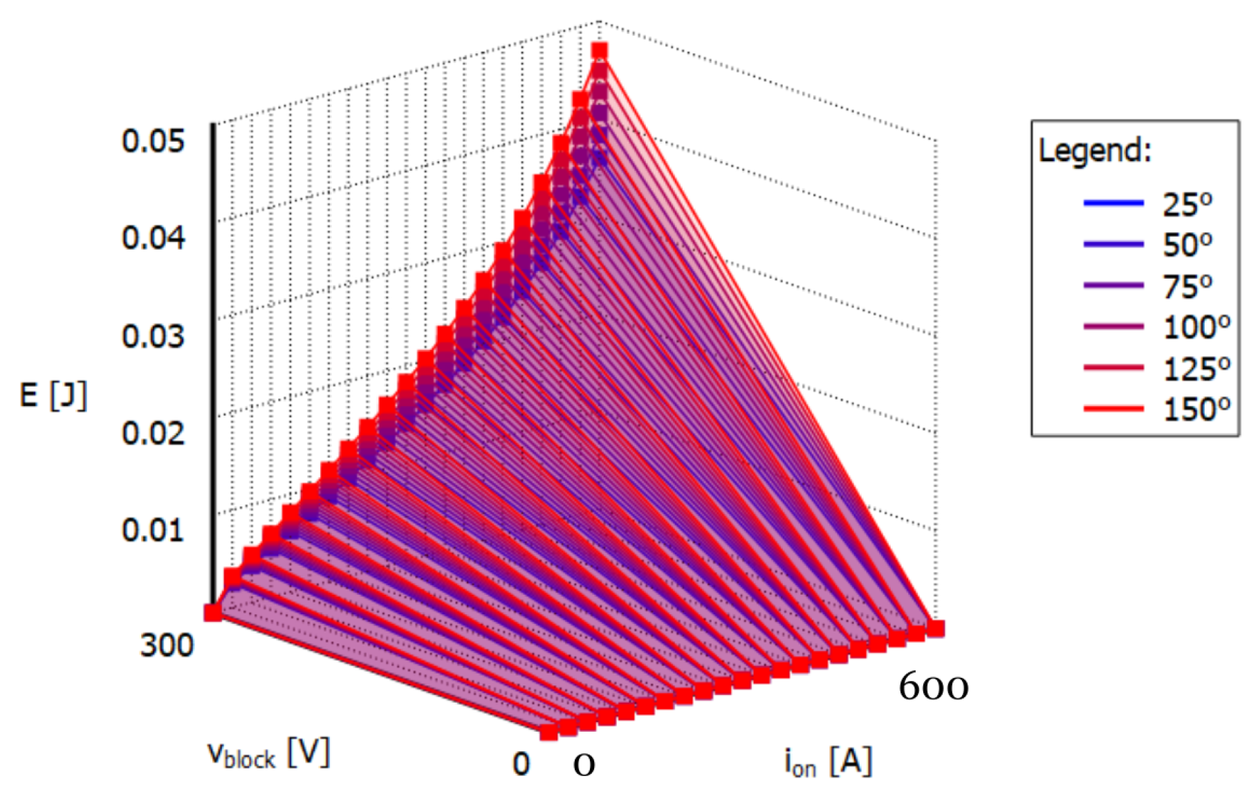
3.3. Switching Loss Calculation
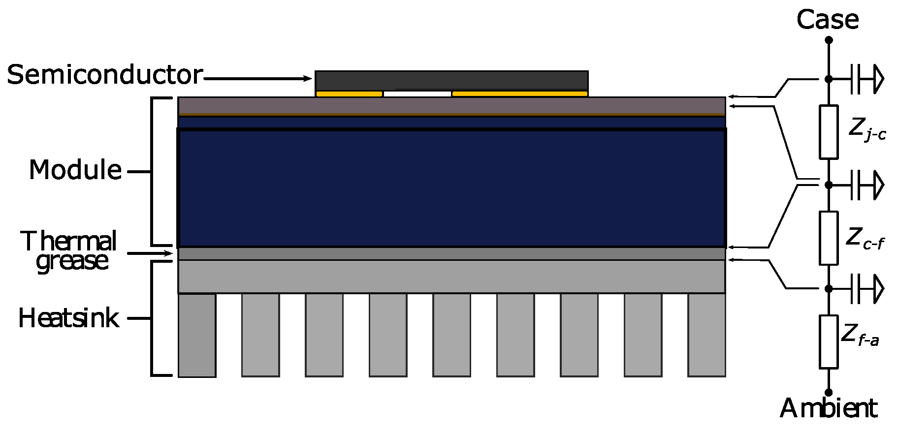
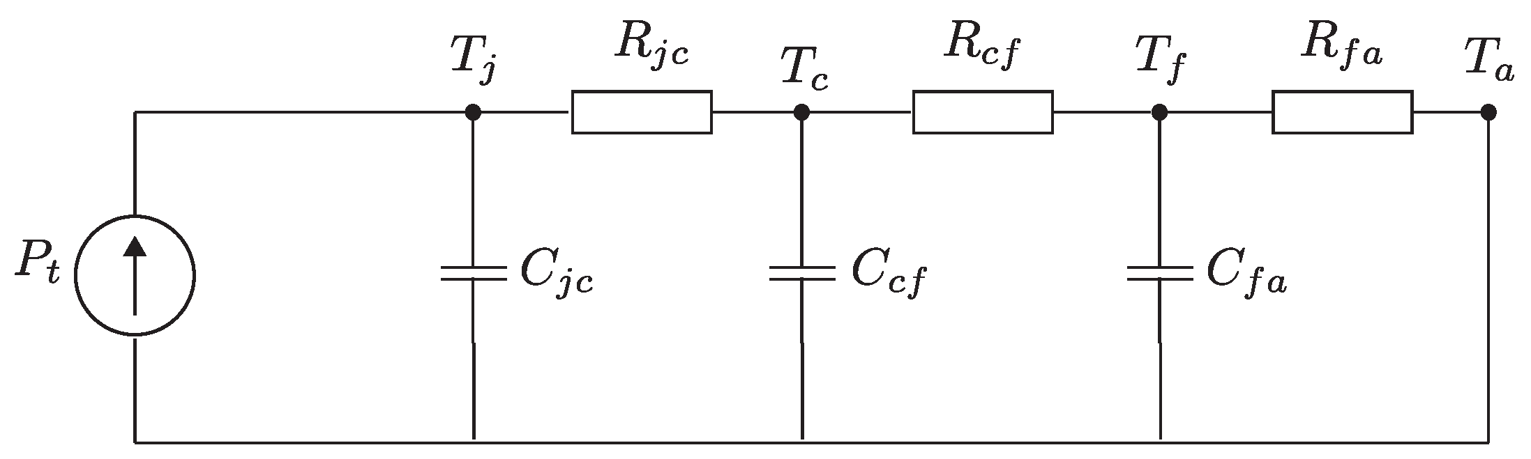
3.4. Thermal Model
4. Induction Machine Dynamic Model
5. Control Schemes
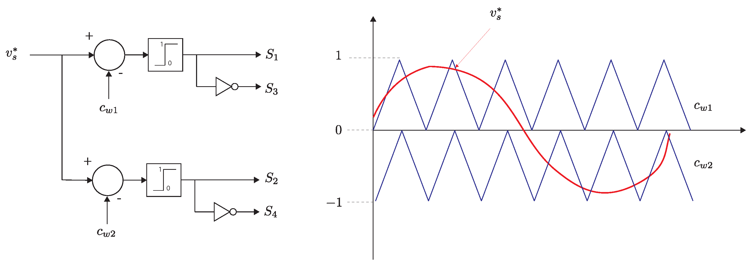
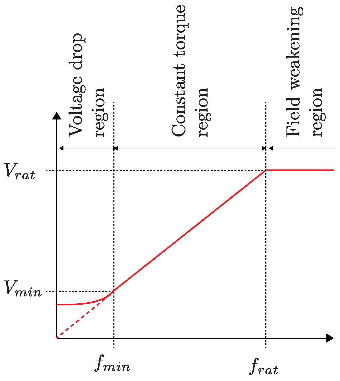
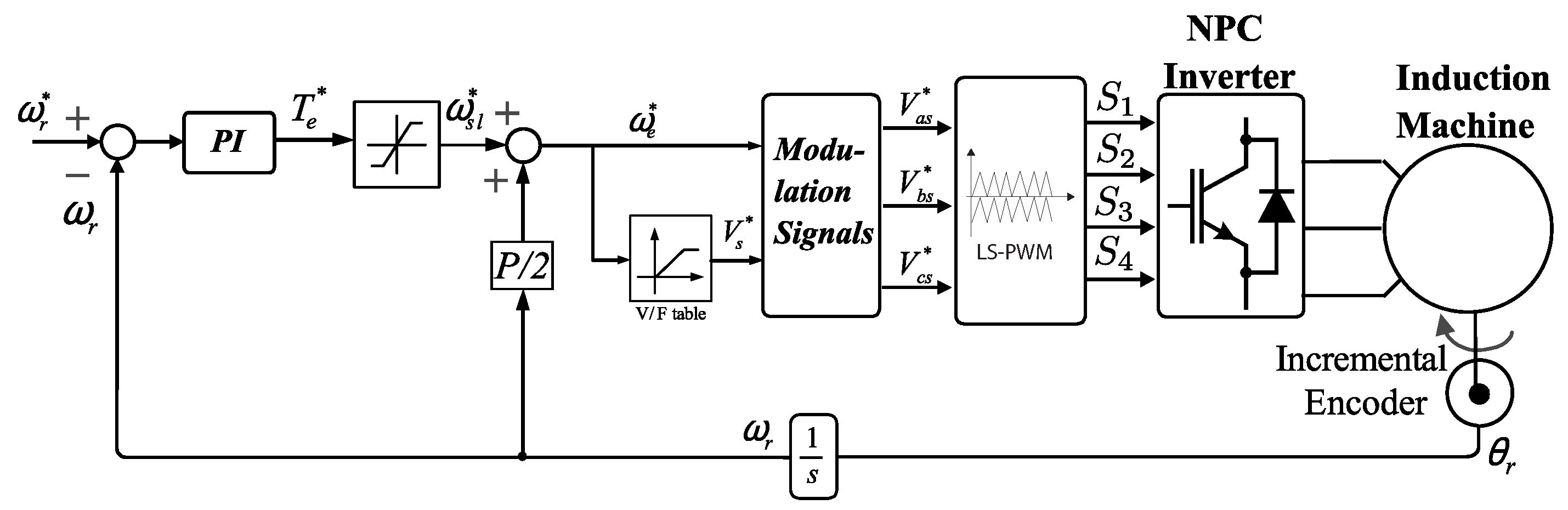
5.1. Scalar Control
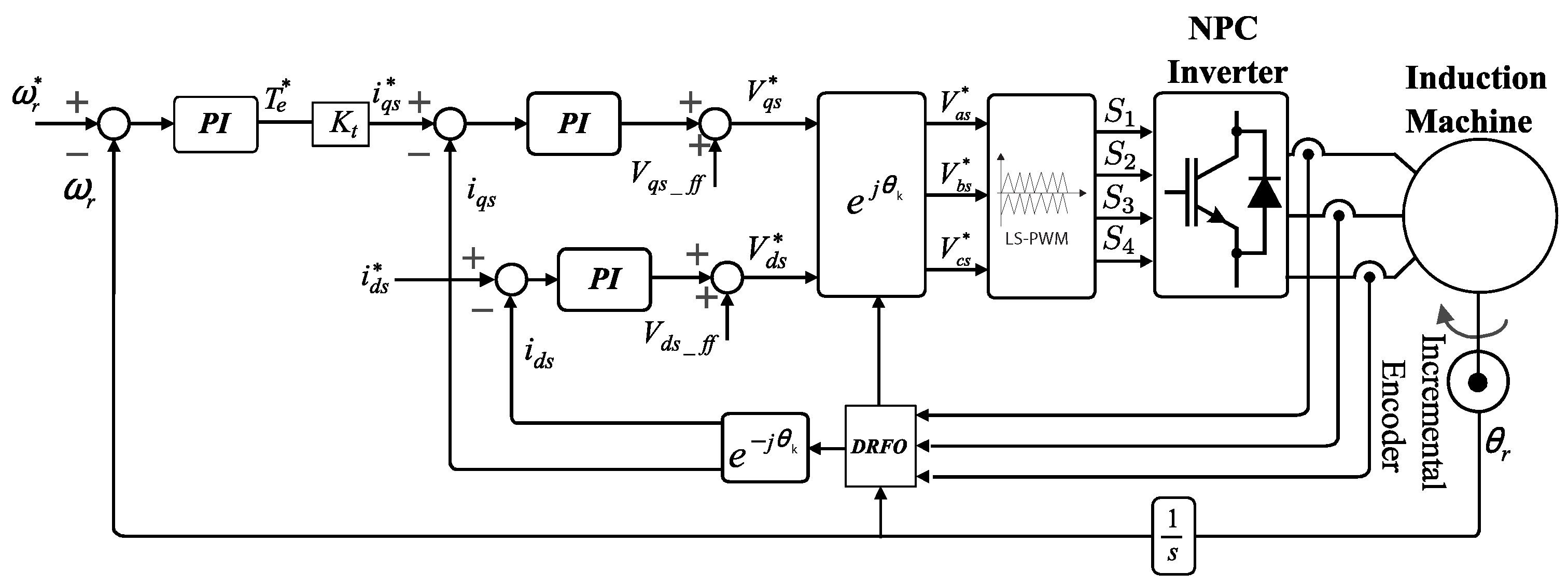
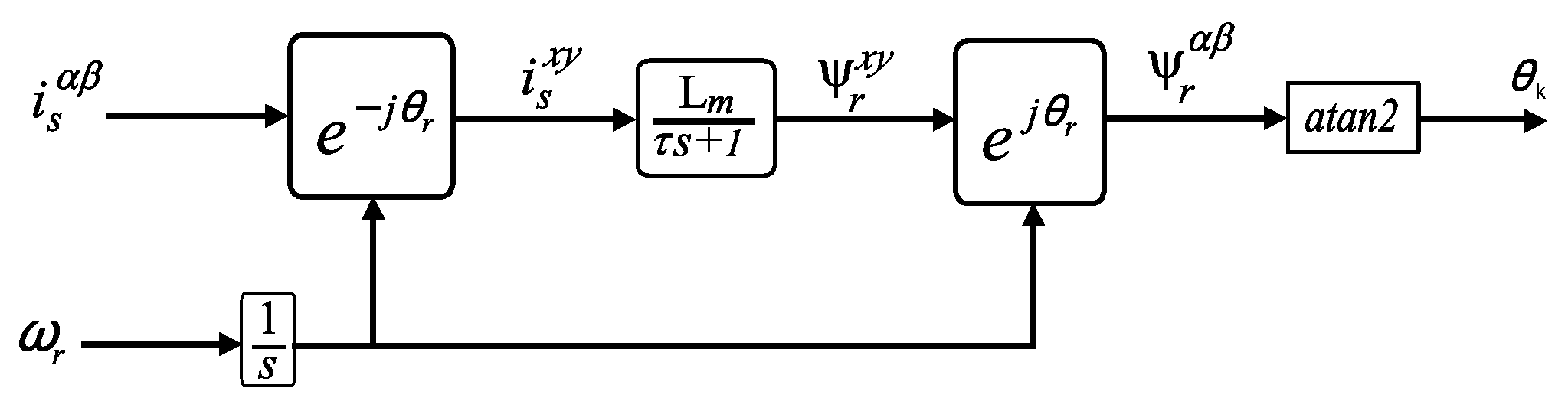
5.2. Field-Oriented Control
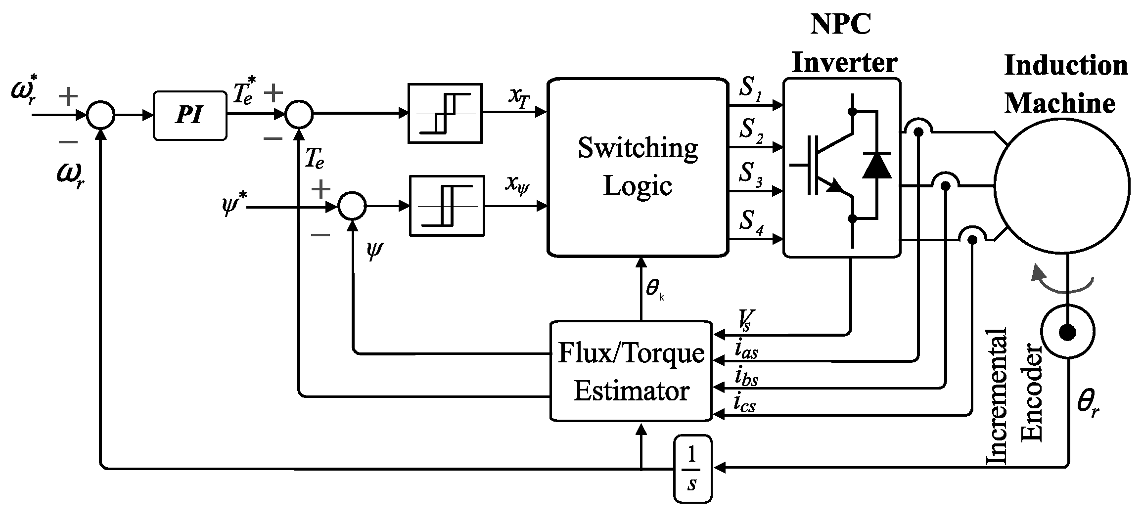
5.3. Direct Torque Control
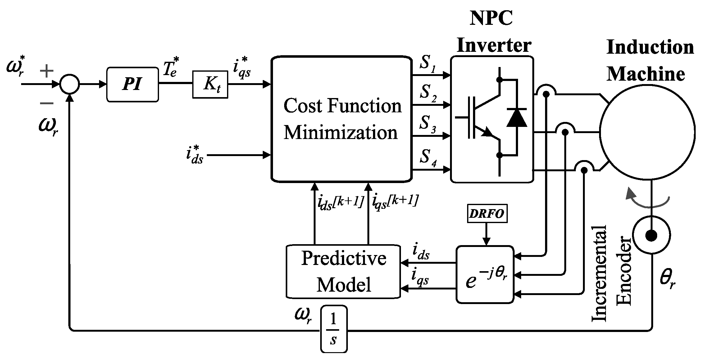
5.4. Model Predictive Control
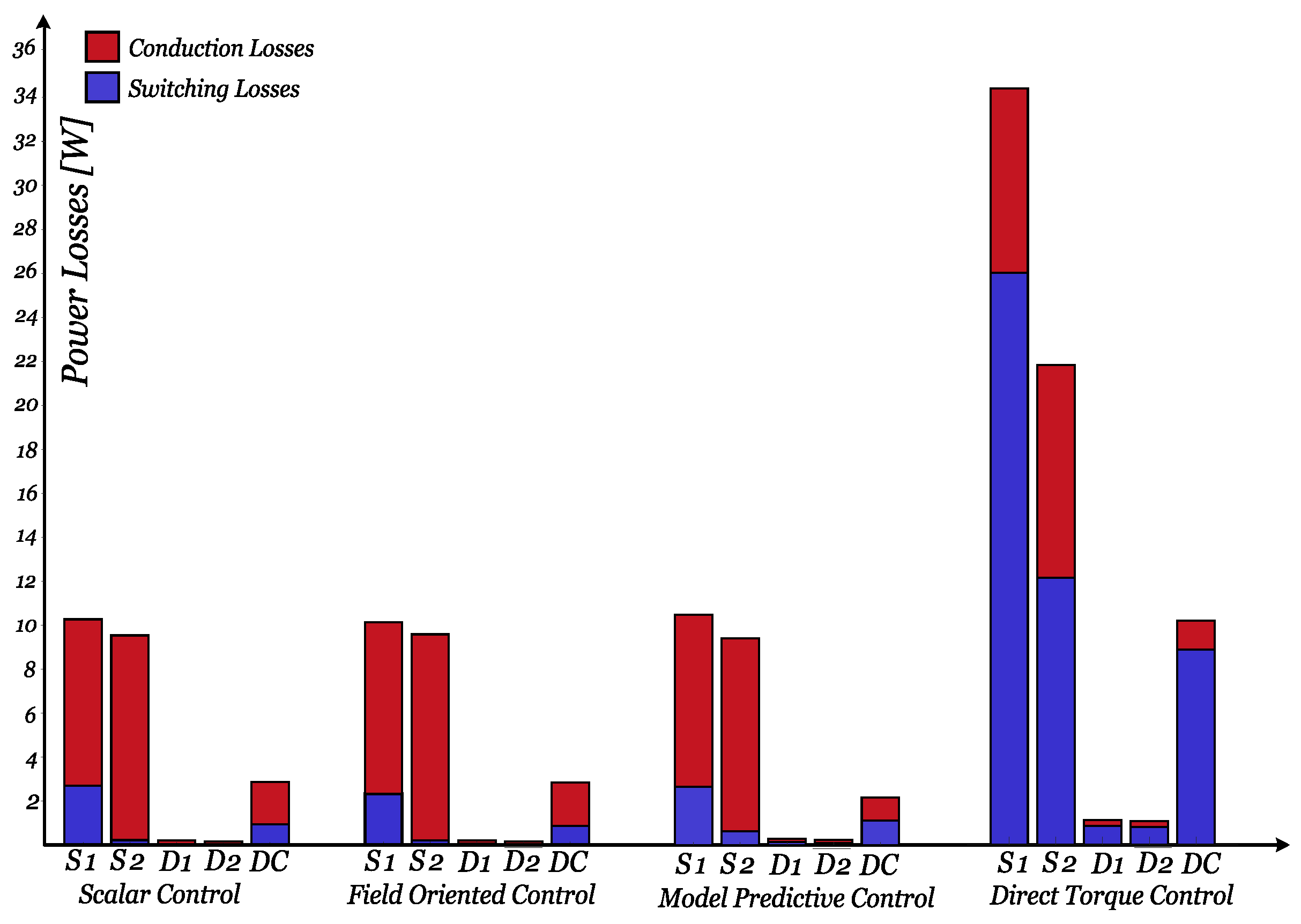
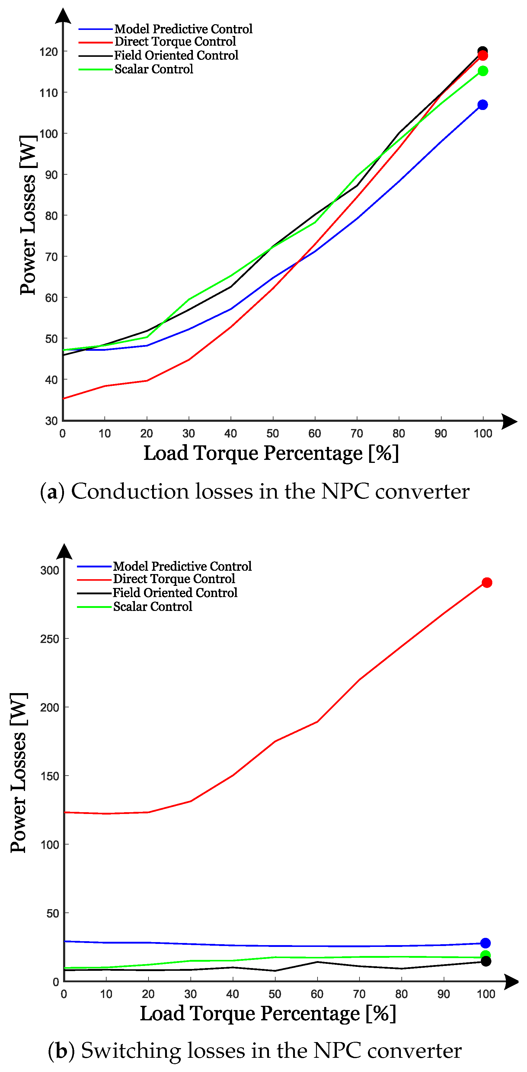
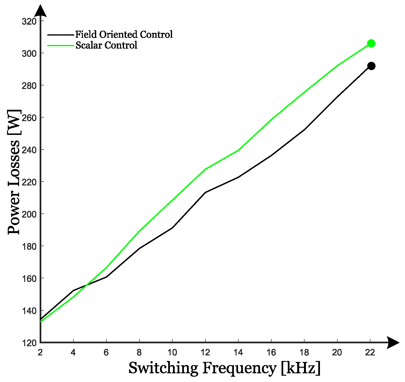
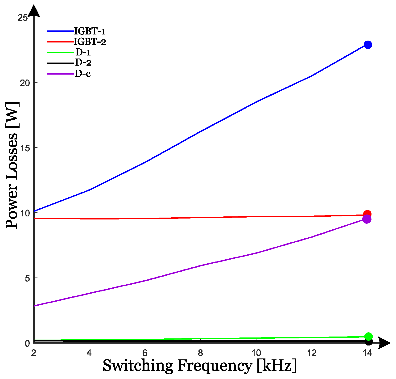
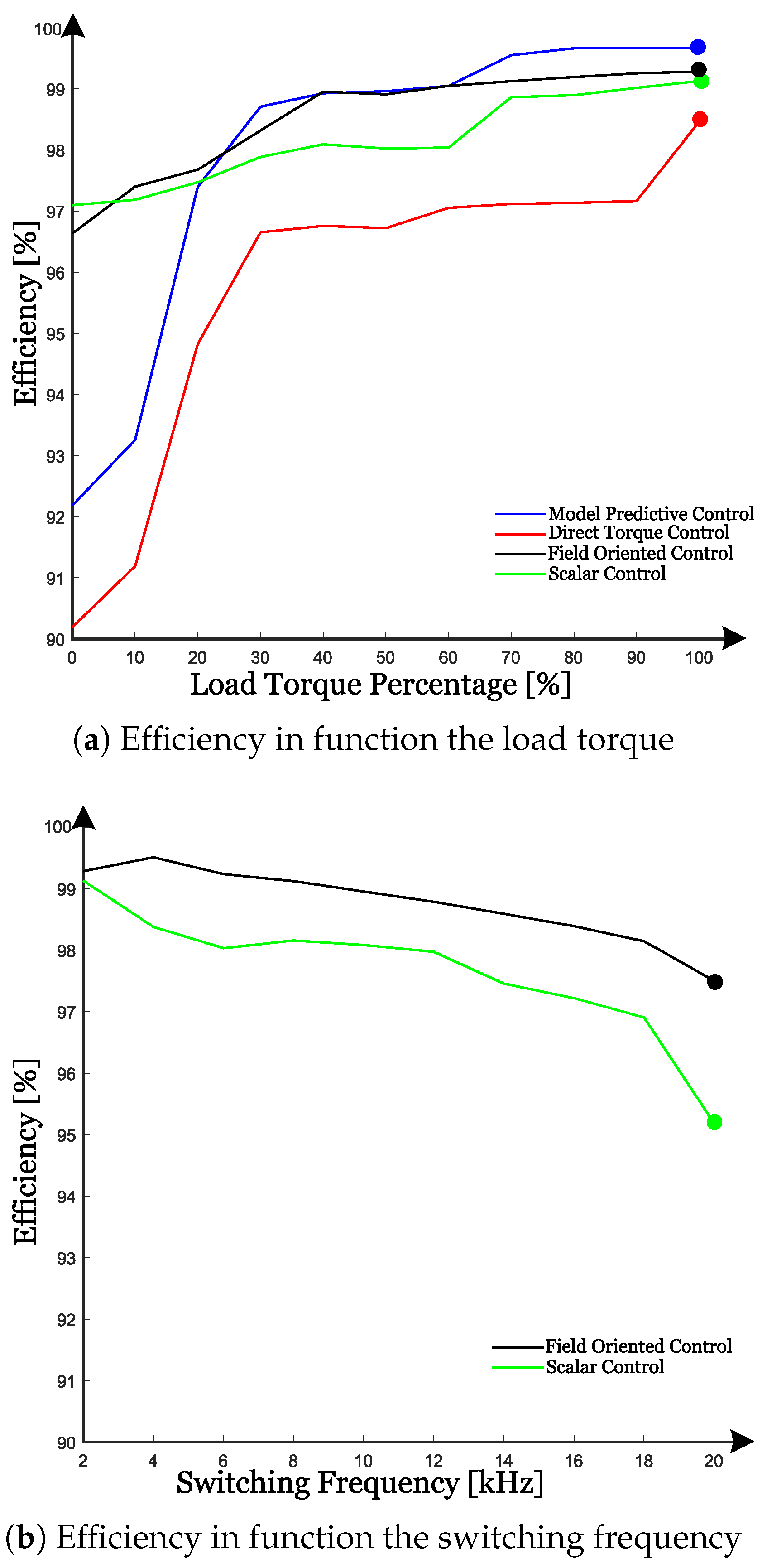
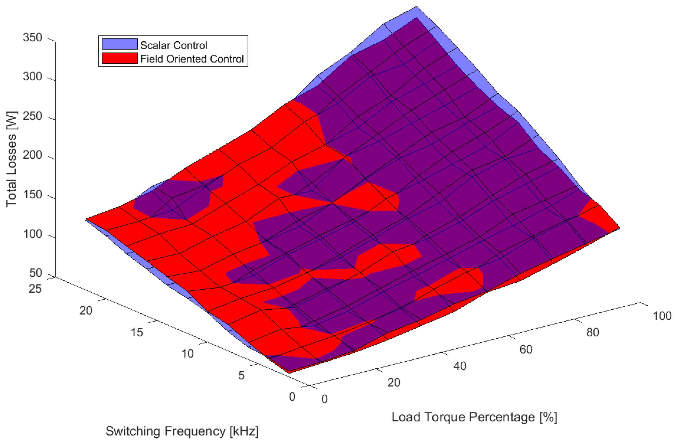
6. Results
7. Discussion
8. Conclusions
Author Contributions
Funding
Data Availability Statement
Acknowledgments
Conflicts of Interest
Abbreviations
| 2L-VSC | two-level voltage source converter |
| 3L-NPC | three-level NPC |
| DTC | direct torque control |
| DRFO | direct reference frame orientation |
| FOC | field-oriented control |
| IM | induction machine |
| LS-PWM | level-shifted PWM |
| MPC | model predictive control |
| M-VSC | multilevel voltage source converter |
| NPC | neutral point clamped |
| PWM | pulse width modulation |
| SC | scalar control |
| SPWM | sinusoidal pulse width modulation |
| SVM | space vector modulation |
| THD | total harmonic distortion |
References
- Pérez, J.R. Predictive Control of Power Converters and Electrical Drives; Wiley: Hoboken, NJ, USA, 2012; p. 399. [Google Scholar]
- Sul, S.K. Control of Electric Machine Drive System; Wiley-IEEE: Piscataway, NJ, USA, 2011; p. 399. [Google Scholar]
- Wu, B.; Narimani, M. High-Power Converters and AC Drives; Wiley-Interscience: Hoboken, NJ, USA, 2017; p. 480. [Google Scholar]
- Alemi, P.; Lee, D.C. Power loss comparison in two- and three-level PWM converters. In Proceedings of the 8th International Conference on Power Electronics—ECCE Asia, Jeju, Republic of Korea, 30 May–3 June 2011; pp. 1452–1457. [Google Scholar] [CrossRef]
- Dieckerhoff, S.; Bernet, S.; Krug, D. Power loss-oriented evaluation of high voltage IGBTs and multilevel converters in transformerless traction applications. IEEE Trans. Power Electron. 2005, 20, 1328–1336. [Google Scholar] [CrossRef]
- Babaie, A.; Karami, B.; Abrishamifar, A. Improved equations of switching loss and conduction loss in SPWM multilevel inverters. In Proceedings of the 2016 7th Power Electronics and Drive Systems Technologies Conference (PEDSTC), Tehran, Iran, 16–18 February 2016; pp. 559–564. [Google Scholar] [CrossRef]
- Andler, D.; Kouro, S.; Perez, M.; Rodriguez, J.; Wu, B. Switching loss analysis of modulation methods used in neutral point clamped converters. In Proceedings of the 2009 IEEE Energy Conversion Congress and Exposition, San Jose, CA, USA, 20–24 September 2009; pp. 2565–2571. [Google Scholar] [CrossRef]
- Kim, T.J.; Kang, D.W.; Lee, Y.H.; Hyun, D.S. The analysis of conduction and switching losses in multi-level inverter system. In Proceedings of the 2001 IEEE 32nd Annual Power Electronics Specialists Conference (IEEE Cat. No.01CH37230), Vancouver, BC, Canada, 17–21 June 2001; Volume 3, pp. 1363–1368. [Google Scholar] [CrossRef]
- Gervasio, F.; Mastromauro, R.A.; Liserre, M. Power losses analysis of two-levels and three-levels PWM inverters handling reactive power. In Proceedings of the 2015 IEEE International Conference on Industrial Technology (ICIT), Seville, Spain, 17–19 March 2015; pp. 1123–1128. [Google Scholar] [CrossRef]
- Artal-Sevil, J.S.; Lujano-Rojas, J.M.; Bernal-Ruiz, C.; Gorrachategui, I.S. Analysis of Power Losses in a Three-Phase Inverter 3L-NPC. Comparison with different PWM Modulation Techniques. In Proceedings of the 2018 XIII Technologies Applied to Electronics Teaching Conference (TAEE), La Laguna, Spain, 20–22 June 2018; pp. 1–9. [Google Scholar] [CrossRef]
- Nabae, A.; Takahashi, I.; Akagi, H. A New Neutral-Point-Clamped PWM Inverter. IEEE Trans. Ind. Appl. 1981, IA-17, 518–523. [Google Scholar] [CrossRef]
- Kouro, S.; Malinowski, M.; Gopakumar, K.; Pou, J.; Franquelo, L.G.; Wu, B.; Rodriguez, J.; Pérez, M.A.; Leon, J.I. Recent Advances and Industrial Applications of Multilevel Converters. IEEE Trans. Ind. Electron. 2010, 57, 2553–2580. [Google Scholar] [CrossRef]
- Kim, D.; Yamamoto, Y.; Nagao, S.; Wakasugi, N.; Chen, C.; Suganuma, K. Measurement of Heat Dissipation and Thermal-Stability of Power Modules on DBC Substrates with Various Ceramics by SiC Micro-Heater Chip System and Ag Sinter Joining. Micromachines 2019, 10, 745. [Google Scholar] [CrossRef] [PubMed]
- Infineon: Semiconductors and System Solutions 2023. Available online: https://www.infineon.com/ (accessed on 20 June 2024).
- Kazmierkowski, M.P. Electric Motor Drives: Modeling, Analysis and Control, R. Krishan, Prentice-Hall, Upper Saddle River, NJ, 2001, xxviii + 626 pp. ISBN 0-13-0910147. Int. J. Robust Nonlinear Control 2004, 14, 767–769. [Google Scholar] [CrossRef]
- Wu, B.; Narimani, M. Control of Induction Motor Drives. In High-Power Converters and AC Drives; Wiley: Hoboken, NJ, USA, 2017; pp. 321–352. [Google Scholar] [CrossRef]
- Hakami, S.S.; Alsofyani, I.M.; Lee, K.B. Direct Torque Control of IM Fed by 3L-NPC Inverter with Simple Flux Regulation Technique. In Proceedings of the 2019 IEEE Student Conference on Electric Machines and Systems (SCEMS 2019), Busan, Republic of Korea, 1–3 November 2019; pp. 1–6. [Google Scholar] [CrossRef]
- Young, H.A.; Marin, V.A.; Pesce, C.; Rodriguez, J. Simple Finite-Control-Set Model Predictive Control of Grid-Forming Inverters with LCL Filters. IEEE Access 2020, 8, 81246–81256. [Google Scholar] [CrossRef]
- Cataldo, P.; Jara, W.; Riedemann, J.; Pesce, C.; Andrade, I.; Pena, R. A Predictive Current Control Strategy for a Medium-Voltage Open-End Winding Machine Drive. Electronics 2023, 12, 1070. [Google Scholar] [CrossRef]
- Cortes, P.; Rodriguez, J.; Quevedo, D.E.; Silva, C. Predictive Current Control Strategy with Imposed Load Current Spectrum. IEEE Trans. Power Electron. 2008, 23, 612–618. [Google Scholar] [CrossRef]
- Wolbank, T.M.; Stumberger, R.; Lechner, A.; Machl, J. Novel approach of constant switching-frequency inverter control with optimum current transient response. In Proceedings of the SPEEDAM 2010, Pisa, Italy, 14–16 June 2010; pp. 803–808. [Google Scholar] [CrossRef]
- Rivera, M.; Kouro, S.; Rodriguez, J.; Wu, B.; Yaramasu, V.; Espinoza, J.; Melila, P. Predictive current control in a current source inverter operating with low switching frequency. In Proceedings of the 4th International Conference on Power Engineering, Energy and Electrical Drives, Istanbul, Turkey, 13–17 May 2013; pp. 334–339. [Google Scholar] [CrossRef]
- Aguirre, M.; Kouro, S.; Rojas, C.A.; Rodriguez, J.; Leon, J.I. Switching Frequency Regulation for FCS-MPC Based on a Period Control Approach. IEEE Trans. Ind. Electron. 2018, 65, 5764–5773. [Google Scholar] [CrossRef]
- Musallam, M.; Johnson, C.M.; Yin, C.; Lu, H.; Bailey, C. In-service life consumption estimation in power modules. In Proceedings of the 2008 13th International Power Electronics and Motion Control Conference, Poznan, Poland, 1–3 September 2008; pp. 76–83. [Google Scholar] [CrossRef]
- Musallam, M.; Johnson, C.M.; Yin, C.; Bailey, C.; Mermet-Guyennet, M. Real-time life consumption power modules prognosis using on-line rainflow algorithm in metro applications. In Proceedings of the 2010 IEEE Energy Conversion Congress and Exposition, Atlanta, GA, USA, 12–16 September 2010; pp. 970–977. [Google Scholar] [CrossRef]
- Musallam, M.; Johnson, C.M. An Efficient Implementation of the Rainflow Counting Algorithm for Life Consumption Estimation. IEEE Trans. Reliab. 2012, 61, 978–986. [Google Scholar] [CrossRef]
- Huang, H.; Mawby, P.A. A Lifetime Estimation Technique for Voltage Source Inverters. IEEE Trans. Power Electron. 2013, 28, 4113–4119. [Google Scholar] [CrossRef]

| 1 | 1 | 0 | |
| 0 | 1 | 1 | 0 |
| 0 | 0 | 0 |
| S.1 | S.2 | S.3 | S.4 | S.5 | S.6 | S.7 | S.8 | S.9 | S.10 | S.11 | S.12 | ||
|---|---|---|---|---|---|---|---|---|---|---|---|---|---|
| 2 | |||||||||||||
| 1 | |||||||||||||
| 1 | 0 | ||||||||||||
| −1 | |||||||||||||
| −2 | |||||||||||||
| 2 | |||||||||||||
| 1 | |||||||||||||
| 0 | 0 | ||||||||||||
| −1 | |||||||||||||
| −2 |
| Parameter | Value | |
|---|---|---|
| NPC Module | ||
| DC-Link Voltage | 600 [V] | |
| Blocking Voltage | 650 [V] | |
| Collector nominal current | 300 [A] | |
| Collector emitter | 1.55 [V] | |
| saturation voltage | ||
| IGBT thermal resistance | 0.16 [K/W] | |
| junction to case | ||
| IGBT thermal resistance | 0.063 [K/W] | |
| case to heat-sink | ||
| Diode thermal resistance | 0.32 [K/W] | |
| junction to case | ||
| Diode thermal resistance | 0.125 [K/W] | |
| case to heat-sinkk | ||
| Squirrel Cage Induction Motor | ||
| Nominal Power | 15 [kW] | |
| Nominal Voltage | 400 [] | |
| Rated speed | 1460 [RPM] | |
| Nominal current | 30 [] | |
| Nominal torque | 98 [Nm] | |
| p | Pole Pairs | 2 |
| Stator Resistance | 0.2147 [] | |
| Stator Leakage Inductance | 0.991 [mH] | |
| Rotor Resistance | 0.2205 [] | |
| Rotor Leakage Inductance | 0.991 [mH] | |
| Magnetizing Inductance | 64.19 [mH] | |
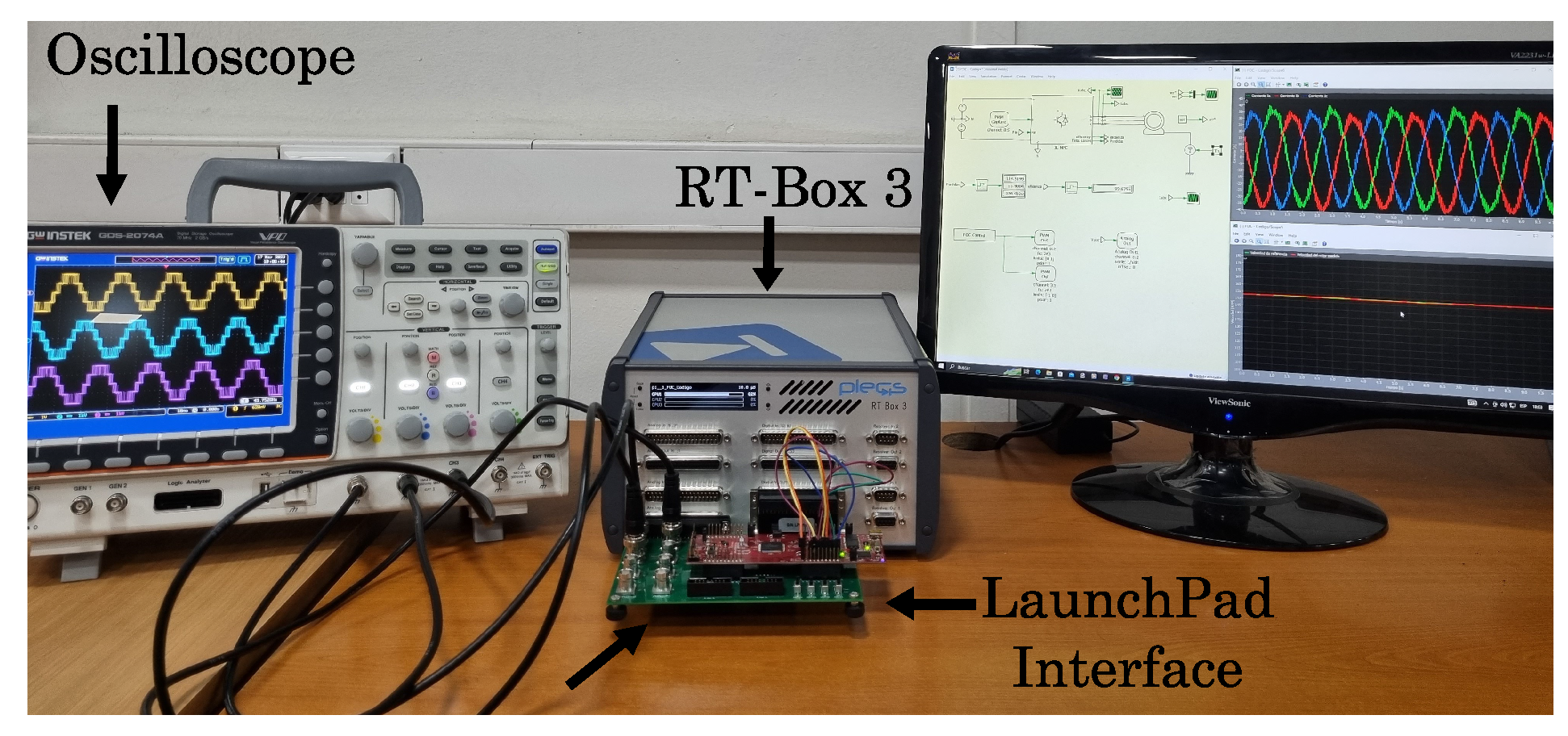
| Real-time RT-Box | ||
| Sampling Time | 10 [μs] | |
| Scalar Control | Field-Oriented Control | Model Predictive Control | Direct Torque Control | |
|---|---|---|---|---|
| 17.3879 | 14.3675 | 27.8165 | 119.1384 | |
| 115.453 | 120.0106 | 107.1836 | 291.134 | |
| 132.841 | 134.3781 | 135.0012 | 410.2724 | |
| 99.12% | 99.1% | 99.09% | 97.26% |
Disclaimer/Publisher’s Note: The statements, opinions and data contained in all publications are solely those of the individual author(s) and contributor(s) and not of MDPI and/or the editor(s). MDPI and/or the editor(s) disclaim responsibility for any injury to people or property resulting from any ideas, methods, instructions or products referred to in the content. |
© 2025 by the authors. Licensee MDPI, Basel, Switzerland. This article is an open access article distributed under the terms and conditions of the Creative Commons Attribution (CC BY) license (https://creativecommons.org/licenses/by/4.0/).
Share and Cite
Reusser, C.A.; Parra, M.; Mino-Aguilar, G.; Gonzalez-Diaz, V.R. Comparison of Induction Machine Drive Control Schemes on the Distribution of Power Losses in a Three-Level NPC Converter. Machines 2025, 13, 227. https://doi.org/10.3390/machines13030227
Reusser CA, Parra M, Mino-Aguilar G, Gonzalez-Diaz VR. Comparison of Induction Machine Drive Control Schemes on the Distribution of Power Losses in a Three-Level NPC Converter. Machines. 2025; 13(3):227. https://doi.org/10.3390/machines13030227
Chicago/Turabian StyleReusser, Carlos A., Matías Parra, Gerardo Mino-Aguilar, and Victor R. Gonzalez-Diaz. 2025. "Comparison of Induction Machine Drive Control Schemes on the Distribution of Power Losses in a Three-Level NPC Converter" Machines 13, no. 3: 227. https://doi.org/10.3390/machines13030227
APA StyleReusser, C. A., Parra, M., Mino-Aguilar, G., & Gonzalez-Diaz, V. R. (2025). Comparison of Induction Machine Drive Control Schemes on the Distribution of Power Losses in a Three-Level NPC Converter. Machines, 13(3), 227. https://doi.org/10.3390/machines13030227