A Novel Bearing Fault Diagnosis Method Based on Improved Convolutional Neural Network and Multi-Sensor Fusion

Abstract

Bearings are key components of modern mechanical equipment. To address the issue that the limited information contained in the single-source signal of the bearing leads to the limited accuracy of the single-source fault diagnosis method, a multi-sensor fusion fault diagnosis method is proposed to improve the reliability of bearing fault diagnosis. Firstly, the feature extraction process of the convolutional neural network (CNN) is improved based on the theory of variational Bayesian inference, which forms the variational Bayesian inference convolutional neural network (VBICNN). VBICNN is used to obtain preliminary diagnosis results of single-channel signals. Secondly, considering the redundancy of information contained in multi-channel signals, a voting strategy is used to fuse the preliminary diagnosis results of the single-channel model to obtain the final results. Finally, the proposed method is evaluated by an experimental dataset of the axlebox bearing of a high-speed train. The results show that the average diagnosis accuracy of the proposed method can reach more than 99% and has favorable stability.

1. Introduction

Bearings are essential components of modern equipment, which directly affect the safety and reliability of equipment [1,2]. In large-scale equipment with harsh working conditions, such as high-speed trains and wind turbines, the harsh operating environment and high-load conditions cause bearings to become one of the key components that are easy to be damaged [3,4]. Therefore, it is of great significance to research effective approaches to diagnose the failure of bearings.

Bearing fault diagnosis can usually be divided into three main steps: data acquisition, feature extraction, and pattern recognition [5]. Due to the convenience of measuring mechanical vibration, bearing fault diagnosis methods based on vibration signals have received a lot of attention [6,7]. Traditional methods of bearing fault diagnosis mainly focus on signal analysis and processing [8,9,10]. This kind of research often adopts Fourier transform, envelope analysis, spectral kurtosis, wavelet transform, and empirical modal decomposition to process the vibration signal. Then, different features are extracted from the processed vibration signals for detecting the health status of bearings, and the common features can be categorized into time-domain features, frequency-domain features, and time-frequency-domain features. Existing studies usually input the features into intelligent classification algorithms to realize the automatic identification of the health status of bearings, and the typical classification algorithms are BP neural networks [11], support vector machines [12,13], and Bayesian classifiers [14]. Although the traditional fault diagnosis methods based on signal processing have been widely used, they rely heavily on manual extraction of fault features, leading to the problems of weak adaptive ability.

Recently, deep learning has developed rapidly which has attracted the attention and application of a large number of scholars [15]. Deep learning models have flexible structures that can extract deep features from input data, eliminating the step of manually extracting and selecting features [16]. The convolutional neural network (CNN) is a typical deep learning model that has been applied in the field of bearing fault diagnosis [17,18,19,20,21,22]. Janssens et al. [17] established a feature learning model based on CNNs that can automatically learn useful features for bearing condition monitoring and fault diagnosis from input data and compared it with the traditional method based on feature extraction by experimental data collected from a bearing test bed. In the comparison experiments, both methods used vibration data collected simultaneously and of the same length, and multiple samples were obtained by adding windows to the vibration data to meet the needs of the classification algorithms and CNNs in terms of the number of training samples. The window used in the traditional method contains 60 s of vibration data and overlaps by 50 percent with its neighboring window, while the window used in the proposed method contains 1 s of vibration data and does not overlap. The experiments on the 4-classification recognition task of bearing health state show that the performance of the feature learning method based on CNN is significantly better than that of the traditional method based on feature extraction, improving the recognition accuracy of bearing faults by about 6%. Zhang et al. [18] revealed a certain similarity between CNN and human discriminative laws by analyzing the Western Reserve University bearing fault dataset, which provides some proof for the application of CNN models within the field of bearing fault diagnosis. Ruan et al. [21] developed a physics-guided CNN (PGCNN) for bearing fault diagnosis. The size of the CNN’s input and the size of the CNN’s kernel depend on the physical characteristics of the bearing acceleration signal, and the validation results using experimental data show that the PGCNN is better than the standard CNN. These research studies have achieved satisfactory results with experimental data having fewer disturbances. However, bearings of complex equipment operate in complex environments, where single-source signals often contain a lot of noise and there is a risk of sensor faults.

In contrast, multi-source signals contain redundant and complementary information, promising to improve the accuracy and reliability of diagnosis. Currently, multi-source information fusion methods have been applied in fault diagnosis of rotating machinery. Based on the level of fusion, it can be grouped into data-level fusion [23,24,25], feature-level fusion [26,27,28] and decision-level fusion [29,30,31]. Data-level fusion directly fuses raw data from multiple sensors and then performs fault diagnosis based on the fused data. Yang et al. [23] proposed a multi-source data-level fusion method based on autoencoder (AE). The method directly fuses vibration signals and motor current signals at the data layer for wind turbine gearbox fault diagnosis. Feature-level fusion fuses the features extracted from the raw data and then performs pattern recognition based on the fused features. Wang et al. [27] calculated 18 statistical features based on the vibration signals collected from each sensor and proposed a hybrid Gaussian variational self-encoder that fuses the same features from different vibration signals at the feature level to realize bearing fault diagnosis and gear fault diagnosis. Decision-level fusion fuses the preliminary diagnosis results obtained based on each single sensor data. The voting method is a classical strategy of decision fusion. Li et al. [30] proposed a bearing fault diagnosis method based on voting strategy and AE. The proposed method used AEs to construct multiple base models and designed a weighted voting strategy based on the classification performance of each base model. Eventually, it realizes bearing fault diagnosis by fusing the pre-diagnosis results of the base models at the decision level. The above research has provided more reliable results and verified the validity of multi-source information fusion.

As mentioned earlier, CNN has the advantages of adaptive feature extraction and pattern recognition, allowing for end-to-end diagnosis. However, it can be affected by incomplete diagnostic information from a single signal. Multi-source information fusion can overcome this issue, decision-level fusion being particularly effective for integrating the pre-diagnosis results obtained based on CNN to guarantee the accuracy and reliability of the diagnosis results. Based on these insights, a bearing fault diagnosis method based on improved CNN and multi-source information fusion is proposed in this paper. The method adopts a framework of diagnosis with decision-level fusion. Firstly, a variational Bayesian inference convolutional neural network (VBICNN) is constructed based on variational Bayesian inference with modifications to the feature extraction method of the CNN, assuming that the latent features extracted by the model obey some prior distribution. The VBICNN is used to train a series of basic diagnosis models based on single-channel signals to provide multiple preliminary diagnosis results. Then, a weighted voting method is used to assign the weights of different basic diagnosis models and calculate the scores of different fault types. Ultimately, the fault type with the highest score is selected as the final prediction.

The rest of this paper is organized as follows. Section 2 briefly describes the theoretical foundations of the methods involved in this paper. Section 3 presents the proposed methodology, explaining the framework, methodology, and implementation process. Section 4 provides an experimental study of axlebox bearings for high-speed trains. Section 5 and Section 6 include the discussion and conclusion, respectively.

2. Theoretical Background

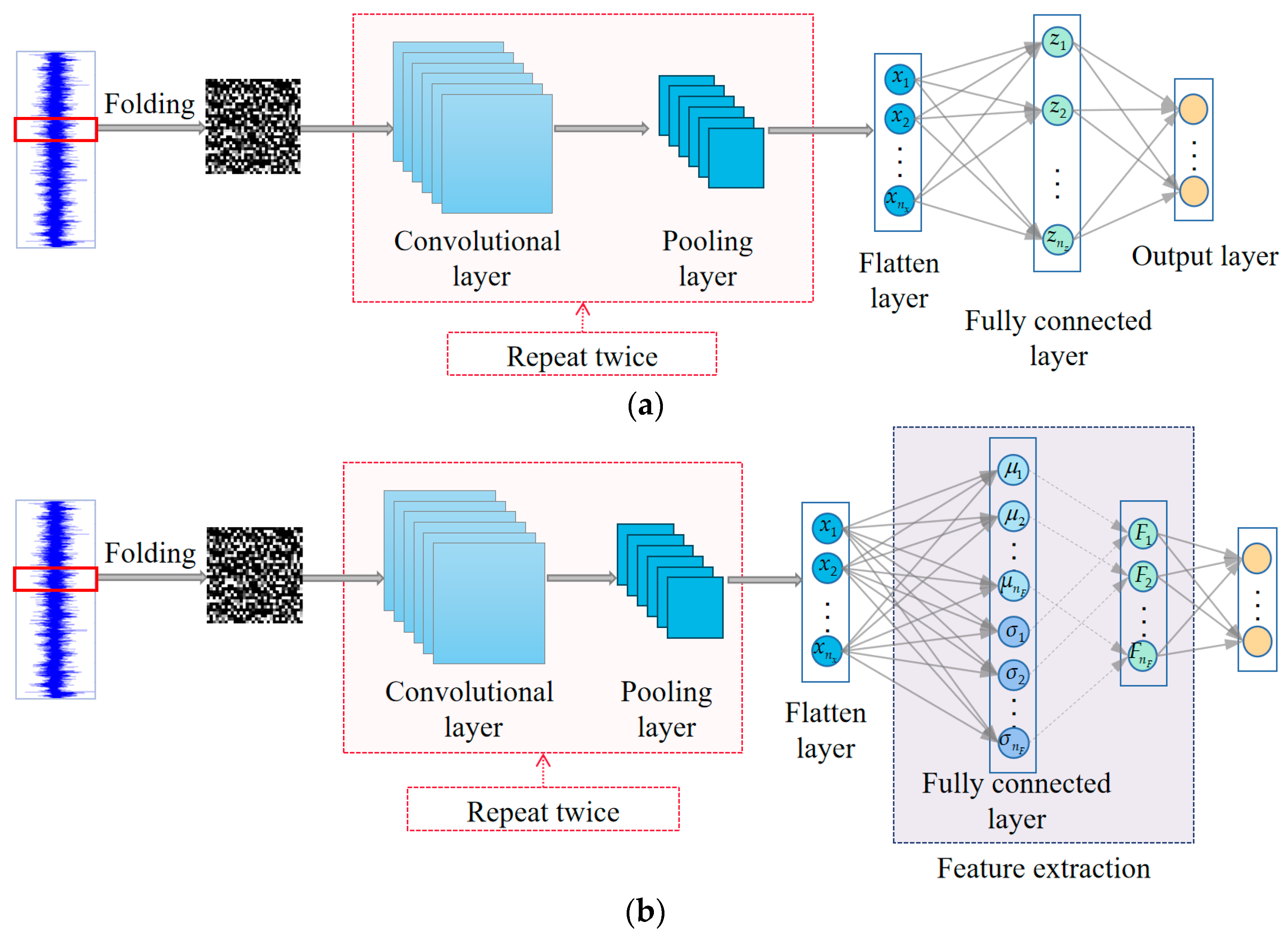
2.1. Convolutional Neural Network

CNN is a common model in the field of deep learning, which was proposed by LeCun et al. [32]. Different from some traditional machine learning algorithms such as support vector machines and BP neural networks, CNNs do not need to extract features manually and can realize “end-to-end” fault diagnosis [33]. The structure of CNN mainly consists of the input layer, convolutional layer, pooling layer, fully connected layer, and output layer [34], as shown in Figure 1.

The convolutional layer serves to extract features mainly from a localized region on the feature map, where various convolution kernels correspond to different feature extractors [35]. The output of the convolutional layer is [34]:

$$Z^p=W^p\otimes X+b^p={\displaystyle \sum _{d=1}^D{W}^{p,d}\otimes X^d+b^p}$$

(1)

where ⨂ denotes the cross-correlation operation, and W^P ∈ R^m×n×D denotes the convolution kernel. The output of the convolutional layer needs to be activated by an activation function and the output Y^P can be expressed as [34]:

$$Y^P=f(Z^P)$$

(2)

where f(·) denotes the activation function. In this paper, the linear rectification function ReLU is used as the activation function.

The pooling layer is usually designed after the convolutional layer and its main role is feature dimensionality reduction. The pooling layer can reduce the number of parameters while extracting the main features, reducing the amount of computation. Average pooling and max pooling are two common forms of calculating the pooling layer [35]. In this paper, we use max pooling, which can be described as follows [35]:

$$Y_{m,n}^d=\underset{i\in R_{m,n}^d}{\max }{x}_i$$

(3)

where x_i is the activation value of each neuron in the region $R_{m,n}^d$ on the feature map.

The fully connected layer is usually set following the convolutional and pooling layers, and its main role is to classify the features based on the features extracted through the convolutional layers and pooling layers. In this paper, the cross-entropy loss function is used and the parameters of each layer of the model are continuously optimized and adjusted with the goal of minimizing the loss function. The expression of the cross-entropy loss function is as follows [21]:

$$L_e(y,\widehat{y})=-{\displaystyle {\sum }_{i=1}^C{y}_i}\log ({\widehat{y}}_i)$$

(4)

where y_i is the true label value of the training sample, and $\widehat{y}$ is the predicted label of the model output.

2.2. Variational Bayesian Inference

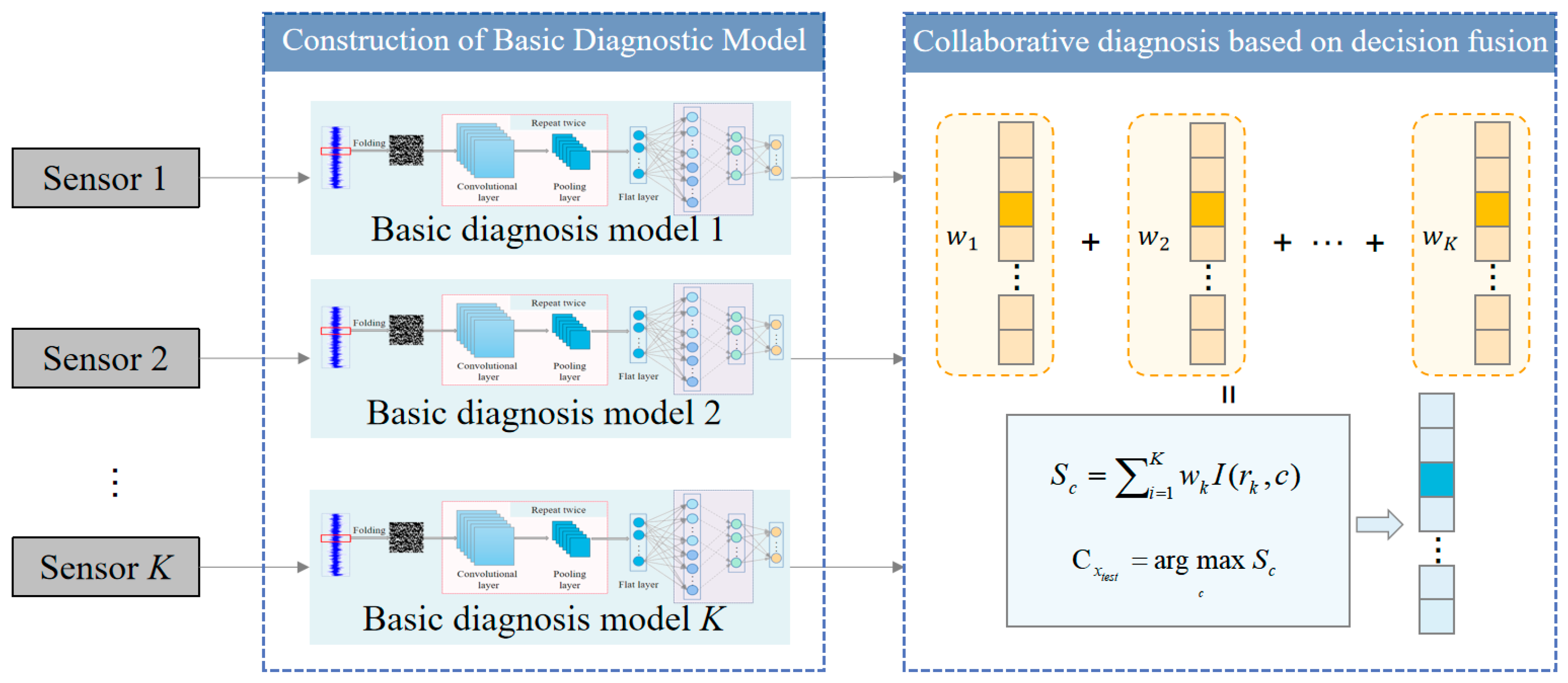
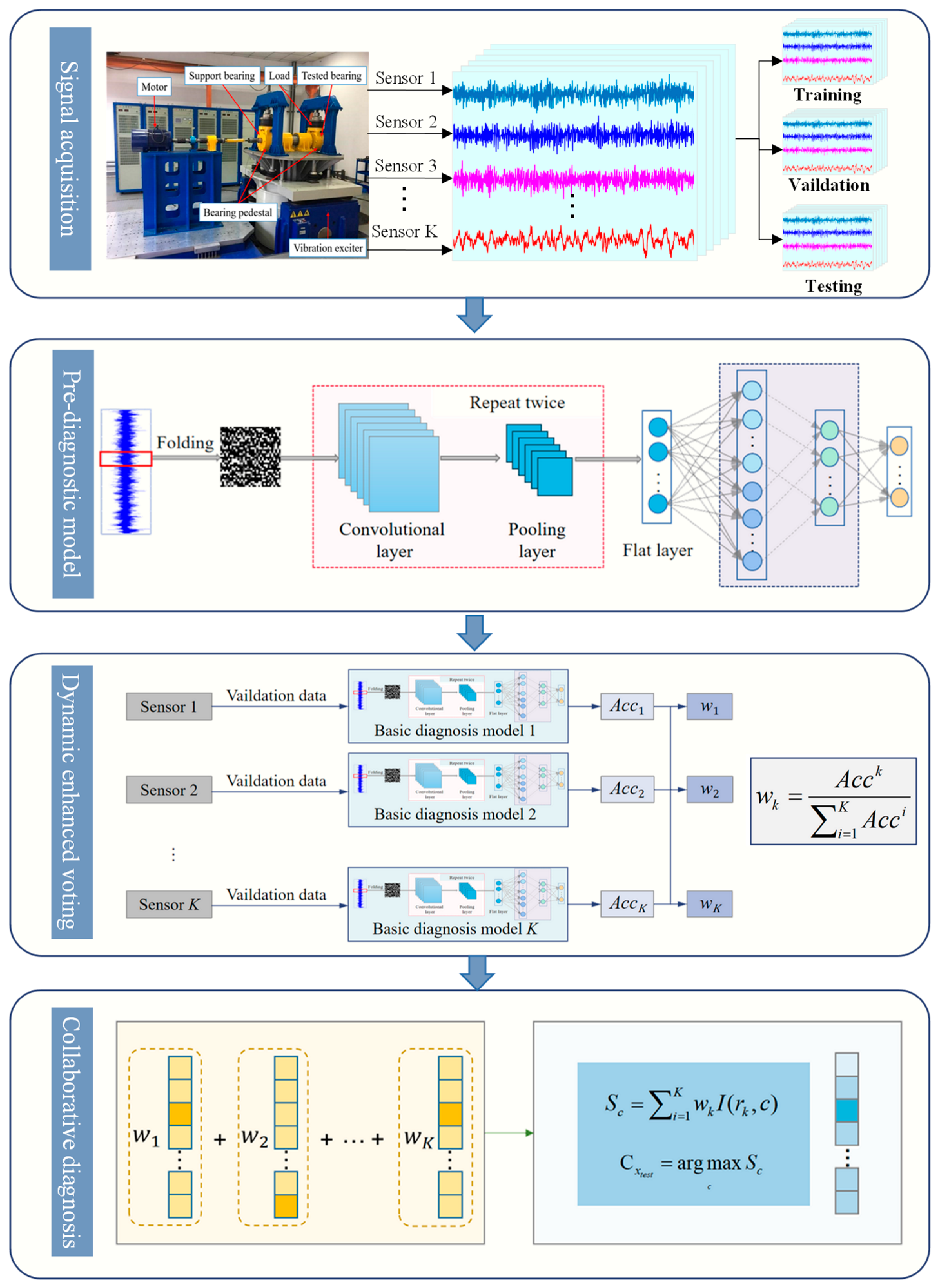
Variational Bayesian inference is a method that combines Bayesian inference and variational inference [36]. Its purpose is to estimate the posterior distribution of latent variables. According to Bayes’ theorem, the posterior distribution p(z|x) of the latent variable z for sample x is as follows [37]:

$$p(\mathit{z}|\mathit{x})={\displaystyle \frac{p(\mathit{x}|\mathit{z})p(\mathit{z})}{p(\mathit{x})}}={\displaystyle \frac{p(\mathit{x}|\mathit{z})p(\mathit{z})}{{\displaystyle \int p(\mathit{x},\mathit{z})d\mathit{z}}}}$$

(5)

where p(x|z) represents the likelihood function of sample x given the latent variable z, p(z) represents the prior distribution of the latent variable z, p(z) represents the marginal likelihood function of sample x, and p(x,z) represents the joint probability distribution of sample x and latent variable z. Obviously, the true posterior distribution p(z|x) of the latent variables is difficult to compute. According to the basic thought of variational inference, it is possible to approximate the complex distribution to be inferred by applying a known simple distribution q(z) [37]. The similarity of the two distributions is measured using the Kullback–Leibler (KL) divergence as follows [37]:

$$D_{KL}(q(\mathit{z})||p(\mathit{z}|\mathit{x}))={\displaystyle \int q(\mathit{z})\log \frac{q(\mathit{z})}{p(\mathit{z}|\mathit{x})}\mathrm{d}\mathit{z}}$$

(6)

To avoid direct computation of the true posterior distribution, Equation (6) can be derived as follows [37]:

$$D_{KL}(q(\mathit{z})||p(\mathit{z}|\mathit{x}))={\displaystyle \int p(\mathit{z})\ln \frac{q(\mathit{z})}{p(\mathit{z},\mathit{x})}\mathrm{d}\mathit{z}+\ln p(\mathit{x})}$$

(7)

where the first term on the right-hand side of the equation is the variational free energy. When the two distributions are equal, the KL divergence takes the value of 0 [38]. Therefore, the objective of the optimization problem is transformed into [39]:

$$\underset{q}{\arg \max }{\displaystyle \int q(\mathit{z})\ln \frac{p(\mathit{z},\mathit{x})}{p(\mathit{z})}}\mathrm{d}\mathit{z}$$

(8)

3. Proposed Method

As mentioned earlier, in complex and changing operating environments, a single monitoring signal for a bearing has the potential problem of incomplete diagnostic information. Existing studies have shown that multi-source signals mounted at different locations or in different directions contain more redundant information that is more beneficial for fault diagnosis [30,31]. Therefore, this paper proposes a new diagnosis method based on multi-source information fusion for bearing fault diagnosis. The proposed method consists of two main parts: the basic diagnostic model construction based on improved CNN, and the decision fusion based on a weighted voting strategy, as shown in Figure 2.

3.1. VBICNN

The structure of the CNN employed in this paper is shown in Figure 3a. The input to the model is the folded vibration signal, and the folding method is referred to in the literature [31]. The model contains two convolution layers and a pooling layer. And the output of the last pooling layer is flattened to obtain a one-dimensional vector. This vector is denoted as the flattened layer and is connected to the fully connected layer. In a standard CNN model, there can be one fully connected layer or multiple fully connected layers. In this paper, a fully connected layer is set up for the last feature extraction before the classifier. Denote the output of the flattened layer neuron as x and the output of the fully connected layer neuron as z. According to the formula for fully connected layer neurons in a standard CNN, the output of the fully connected layer is [34]:

$$\mathit{z}=f_{\mathrm{FC}}({\mathit{W}}_{\mathrm{FC}}\mathit{x}+{\mathit{b}}_{\mathrm{FC}})$$

(9)

where W_FC and b_FC are the weight matrix and bias vector from the flat layer to the fully connected layer, respectively, and f_FC(·) is the activation function of the fully connected layer. To avoid confusion, note the final extracted feature as F. In a standard CNN, the output of the fully connected layer is the final extracted feature, F = z. Finally, the feature F is connected to a Softmax classifier for bearing fault type identification.

Further, in order to enhance the nonlinear mapping ability of the model and the deep feature extraction ability of the fully connected layer, variational Bayesian inference is introduced into the feature extraction of the fully connected layer of the CNN model, forming the VBICNN model, as shown in Figure 3b. In the model training process, the fully connected layer is used to estimate the posterior distribution of the feature F. This means that the neurons of the fully connected layer represent the parameter values of the posterior distribution of the feature F and no longer the value of the feature, F ≠ z. Following the ideology of variational Bayesian inference, a simple known distribution such as a Gaussian distribution can be used to approximate the true posterior distribution. So, assume that the feature F = {F_i} follows Gaussian distribution, $z_i~N({\mu }_i,{\sigma }_i^2)$. Then, the output z of the fully connected layer is:

$$\mathit{z}={[z_1,\cdots ,z_{n_F},z_{n_F+1},\cdots ,z_{2n_F}]}^{\mathrm{T}}={[{\mu }_1,\cdots ,{\mu }_{n_F},{\sigma }_1,\cdots ,{\sigma }_{n_F}]}^{\mathrm{T}}$$

(10)

where n_F is the number of features. Combined with Equation (9), the formula for the parameter values is obtained:

$${[{\mu }_1,\dots ,{\mu }_{n_F},{\sigma }_1,\dots ,{\sigma }_{n_F}]}^T=f(\mathit{W}{\mathit{z}}^{F-1}+\mathit{b})$$

(11)

And then random sampling is performed to generate the feature F. Finally, the feature F is input into the Softmax classifier for bearing fault type identification.

It can be found that on the basis of the optimization objective of the standard CNN model, the VBICNN model adds the constraints of simple distribution and true posterior distribution in variational Bayesian inference. Therefore, the optimization objective of variational Bayesian inference is added to the cross-entropy damage function shown in Equation (4), to form the loss function of the VBICNN model as follows:

$$L_{\mathrm{VBCNN}}(\mathit{x},\mathit{y})=L_e(\widehat{\mathit{y}},\mathit{y})+\beta ·D_{KL}(q(\mathit{z})||p(\mathit{z}|\mathit{x}))$$

(12)

where β is the weight of the error in the distribution of learning features.

3.2. Decision-Level Fusion Method Based on Weighted Fusion Strategy

Assume that the signals come from K channels and that there are C fault types to be recognized. The signals of each channel are divided into training, validation, and test data. After the base VBICNN models are obtained using the training data, validation samples are used to determine the weights of each base VBICNN. In this paper, we assign weights based on the overall validation accuracy of the base model.

Noting that VBICNN_k is the kth base model trained with the kth channel signal, its validation accuracy Acc_k on the validation set is calculated as follows [31]:

$$Ac{c}^k={\displaystyle \frac{T_k}{N_k}}$$

(13)

where N_k is the number of validation samples for the kth channel, and T_k is the number of validation samples in which the diagnosis is correct. Based on this, the weight matrix of all VBICNNs is obtained [40]:

$$\mathit{w}={\left[w_1,w_2,\cdots ,w_K\right]}^T={\left[{\displaystyle \frac{Ac{c}^1}{{\sum }_{i=1}^{K}Ac{c}^i}},{\displaystyle \frac{Ac{c}^2}{{\sum }_{i=1}^{K}Ac{c}^i}},\cdots ,{\displaystyle \frac{Ac{c}^K}{{\sum }_{i=1}^{K}Ac{c}^i}}\right]}^T$$

(14)

Combining the diagnostic results of each channel further, the score for each fault type is calculated as follows [31]:

$$\begin{array}{cc}{S}_c={\sum }_{i=1}^K{w}_{k}I(r_k,c)& c=1, 2,\cdots ,C\end{array}$$

(15)

$$I(r_k,c)=\left\{\begin{array}{cc}1& r_k=c\\ 0& r_k\ne c\end{array}\right.$$

(16)

where is the preliminary diagnosis of the kth VBICNN.

Ultimately, the type with the highest score is selected as the final result of the diagnosis, as follows [31]:

$${\mathrm{C}}_{x_{test}}=\underset{c}{\mathrm{a}\mathrm{r}\mathrm{g} \mathrm{m}\mathrm{a}\mathrm{x}} S_c$$

(17)

3.3. Flow of the Proposed Method

The process of the proposed method is summarized in Figure 4. The specific steps are as follows.

Step 1: Data acquisition. Collect multi-channel vibration signals of mechanical equipment in different operating conditions. The data from each channel is divided into training samples, validation samples and testing samples.

Step 2: Construction of a series of basic VBICNNs. Set the structure and hyperparameters of the VBICNN, and input training samples into the VBICNN to update the parameters.

Step 3: Assigning weights to the basic VBICNNs. Validation samples are fed into the trained basic VBICNNs to calculate the validation accuracy of each VBICNN. Based on the validation accuracy, calculate the weight matrix w of basic VBICNNs.

Step 4: Validation of the proposed method by testing samples. Input the testing samples into a series of trained basic VBICNNs to obtain a series of pre-diagnostic results. Calculate the score of each fault type according to the weight matrix w to obtain the final diagnosis result.

4. Experimental Study

In order to verify the feasibility and effectiveness of the proposed method, multi-channel vibration signals from the high-speed train bearing test bench of Southwest Jiaotong University were used for the experiments.

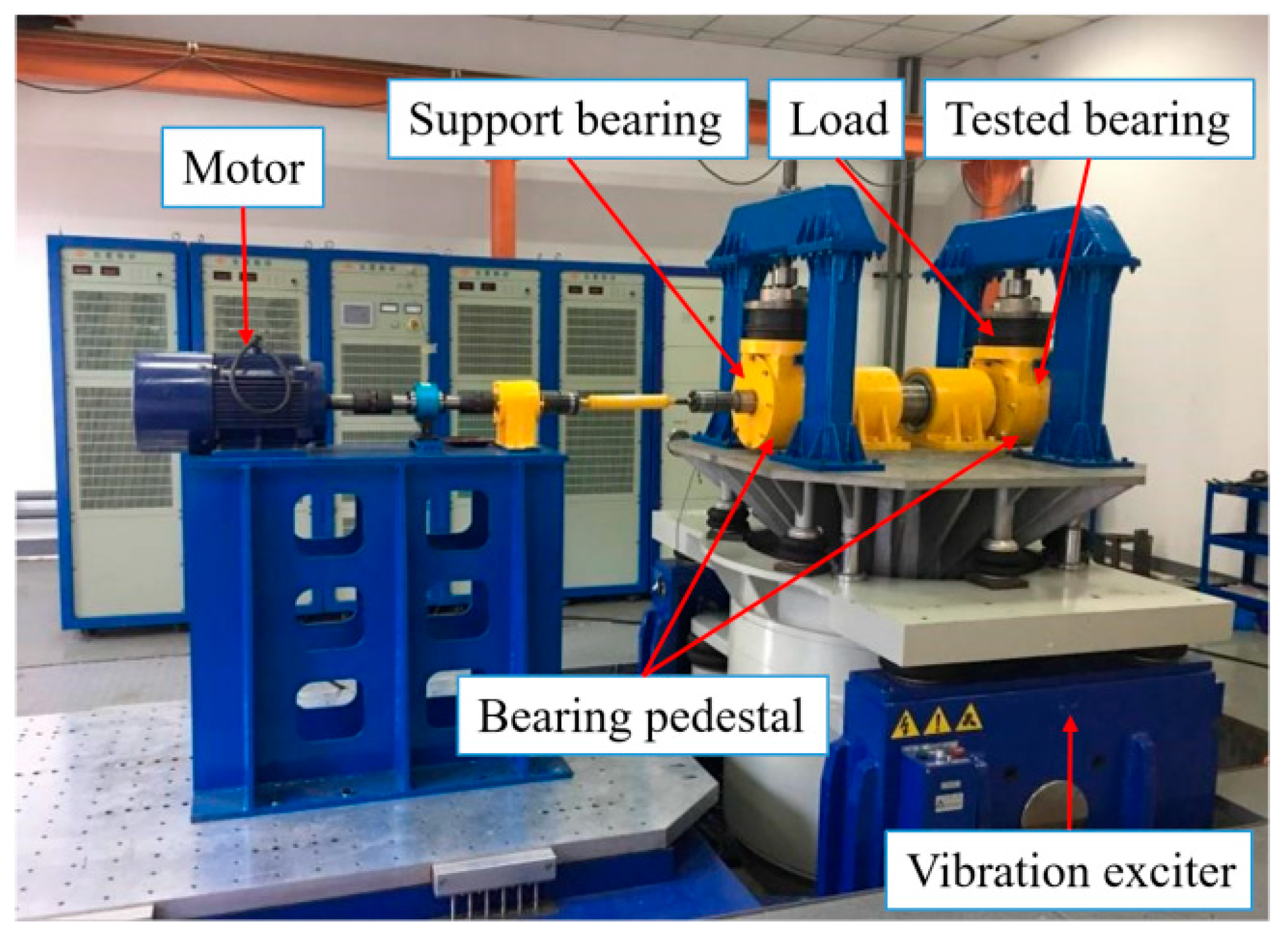
4.1. Experimental Setup

The test bed for the axlebox bearing of the high-speed train of Southwest Jiaotong University is shown in Figure 5. The test device is composed of a motor, support bearing, tested bearing, bearing pedestal, and exciter. The exciter is used to simulate the wheel-rail excitation in the real train operating environment. In the data collection process, the real operating conditions can be simulated by applying the rotating speed, static load force, and excitation frequency to the bearing.

The parameters of the axlebox bearings used are shown in

Table 1. Parameters of the axlebox bearing.

Inner race Diameter	Pitch Circle Diameter	Roller Diameter	Roller Number	Contact Angle (°)
130 mm	184 mm	27 mm	17	0

. In this case, a tri-axis vibration accelerometer was used to acquire the signals in the (x, y, z) direction at the surface of the tested bearing. Noted in order as channels 1–3. In the process of data acquisition, the speed is 1100 rpm, the load is 1200 kg, the excitation frequency is 10 Hz, and the sampling frequency is 25.6 kHz. In addition, A total of nine bearing fault types were considered, including normal, inner race fault, outer race fault, cage fault, roller fault, poor grease uniformity, compound faults (inner race and outer race), compound faults (outer race and roller) and compound faults (outer race and grease), as shown in Figure 6. The labels for these 9 fault types are noted in order as 1–9. There are 400 samples for each fault type: 280 training samples, 40 validation samples, and 80 test samples.

4.2. Structural Design of the Model

In this case, the VBICNN of each channel uses the same structure, as shown in

Table 2. Parameters of the VBCNN.

Description	Number of Nodes	Config
Input layer	32 × 32 × 1	-
The first convolutional layer	32 × 32 × 8	5@8/Stride(1,1)/Relu
The first pooling layer	8 × 8 × 8	Stride(4,4)
The second convolutional layer	8 × 8 × 16	5@16/Stride(1,1)/Relu
The second pooling layer	2 × 2 × 16	Stride(2,2)
Flatten layer	64	-
feature extraction layer	32	Tahn
Output layer	9	-

. The structure of VBICNN was obtained by adjusting the structure and parameters of the CNN models that have been repeatedly validated in the industry, consisting of two convolutional layers, two pooling layers, and a fully connected layer. The number of extracted features is 32. The model is trained using the Adam optimizer with a minimum batch size of 128 and an initial learning rate of 0.01. The β in Equation (12) is set to 0.001.

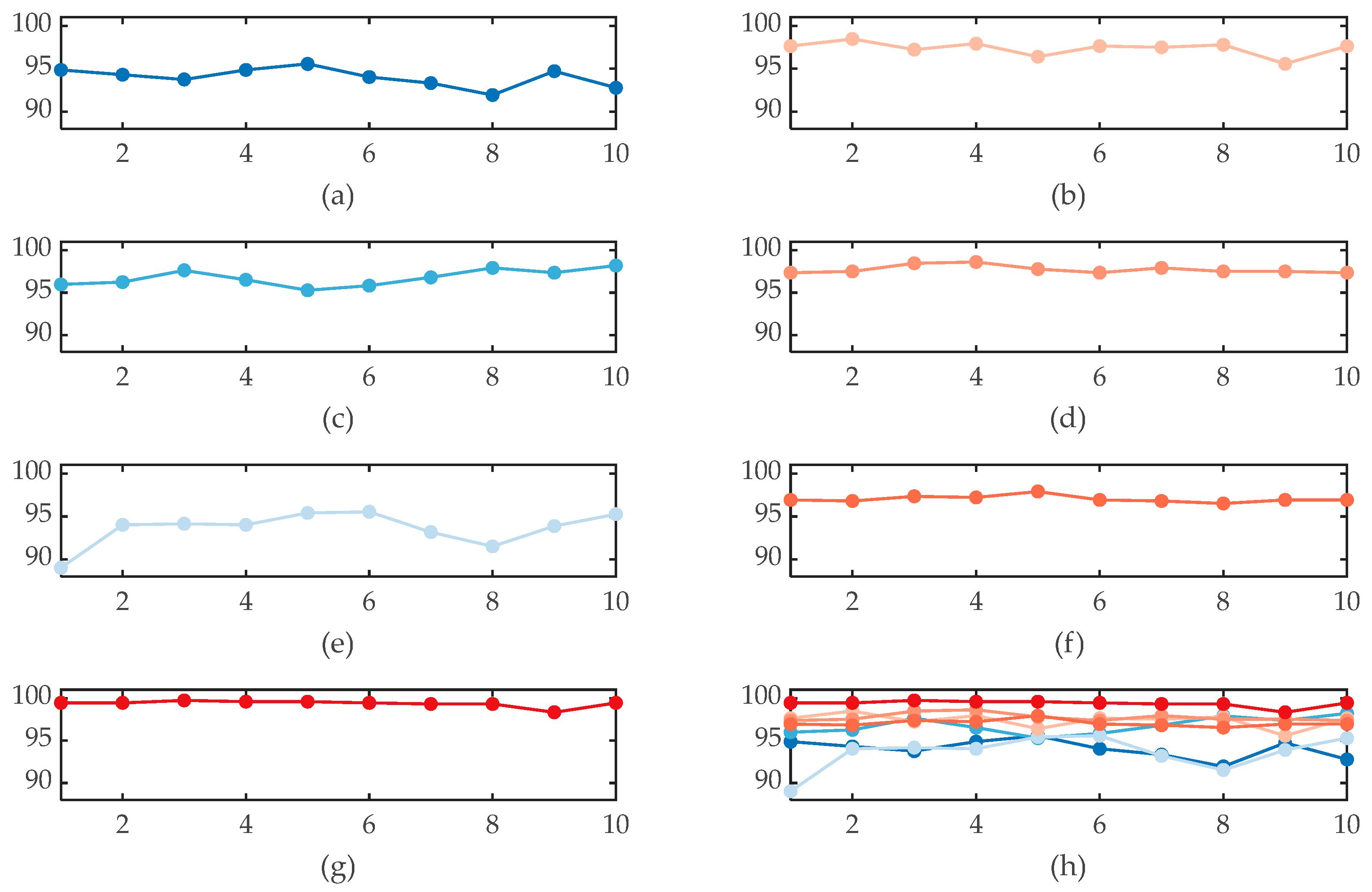
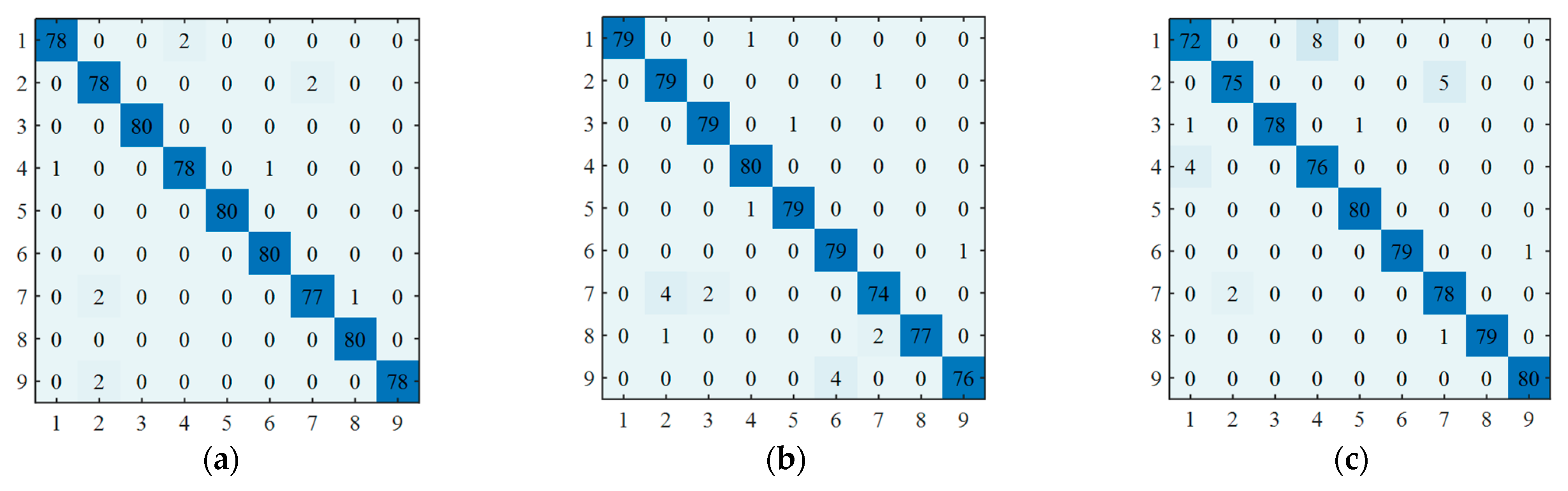
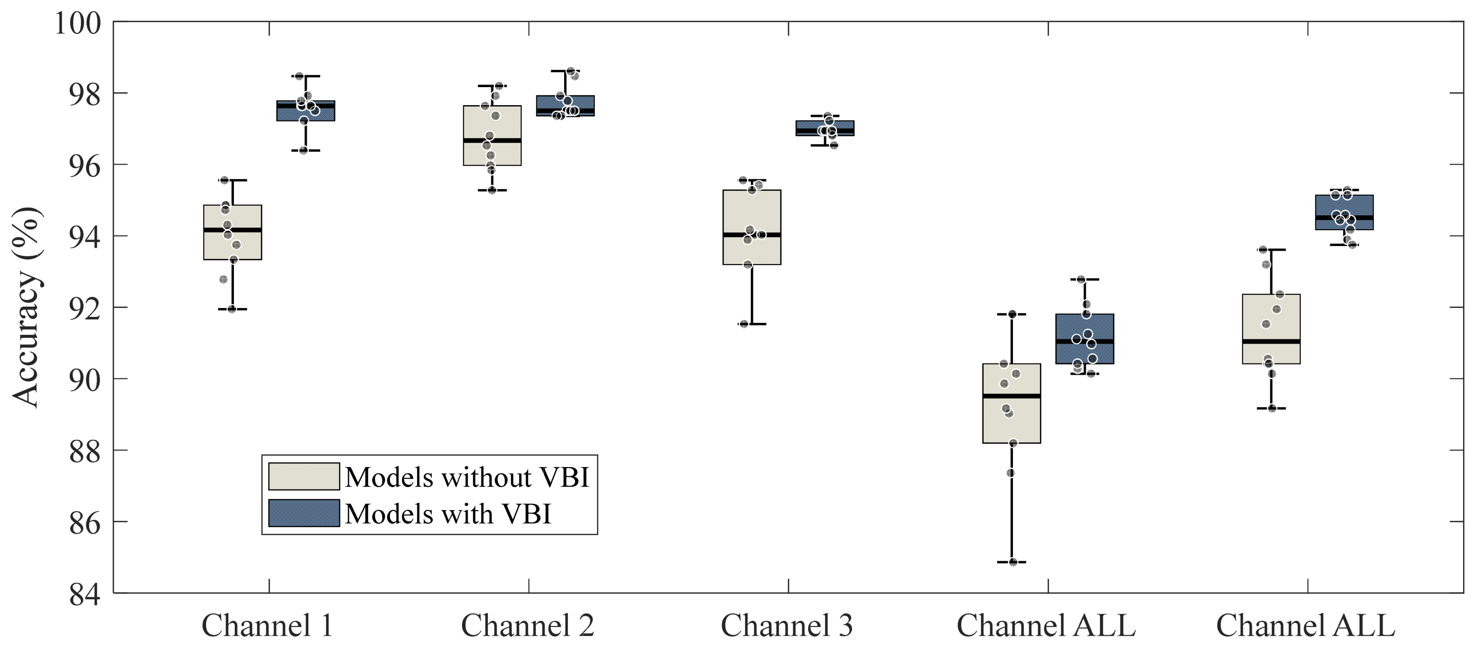
4.3. Ablation Experiment and Results

To validate the effectiveness and necessity of the method proposed in this paper, ablation experiments were carried out.

First, single-channel signals are used as inputs to the models to train the CNN model and the VBICNN model, which obtained three trained CNNs and three trained VBICNNs. By comparing the diagnostic accuracies of CNNs and VBICNNs, the necessity of an improved CNN model using Bayesian variational inference is verified. Then, a decision-level fusion strategy is used to collaborate the diagnostic results of single-channel signals to validate the necessity of collaborative diagnosis of multi-channel signals. Considering the possibility of chance in the experimental results, 10 repeated experiments were carried out and the results are shown in Figure 7, with the average accuracy and standard deviation detailed in

Table 3. Fault diagnosis results using different models and different signals.

Model	Fusion Strategy	Testing Accuracy
		Average Accuracy	Standard Deviations
CNN	Channel 1	94.01%	1.0925
	Channel 2	96.78%	0.9729
	Channel 3	93.61%	2.0020
VBCNN	Channel 1	97.38%	0.8283
	Channel 2	97.74%	0.4630
	Channel 3	97.04%	0.3823
Proposed method	Channel All	99.37%	0.3829

.

Comparing (a) with (b), (c) with (d), and (e) with (f) in Figure 7, it can be found that the diagnosis accuracy of the VBICNN is always higher than that of the CNN when a single-channel signal is used as the model input. Observing the diagnosis results of CNN and VBICNN in Table 3, the average accuracy provided by VBICNN in channels 1 to 3 is 97.38%, 97.74%, and 97.04% in that order, all of which are higher than the results using CNN, and the variance is much smaller, which indicates that the model is more stable. Meanwhile, comparing the proposed method with the VBICNN model with a single channel. As shown in Table 3, the accuracy of the proposed method is 99.28%, which is significantly higher than the VBICNN with a single channel.

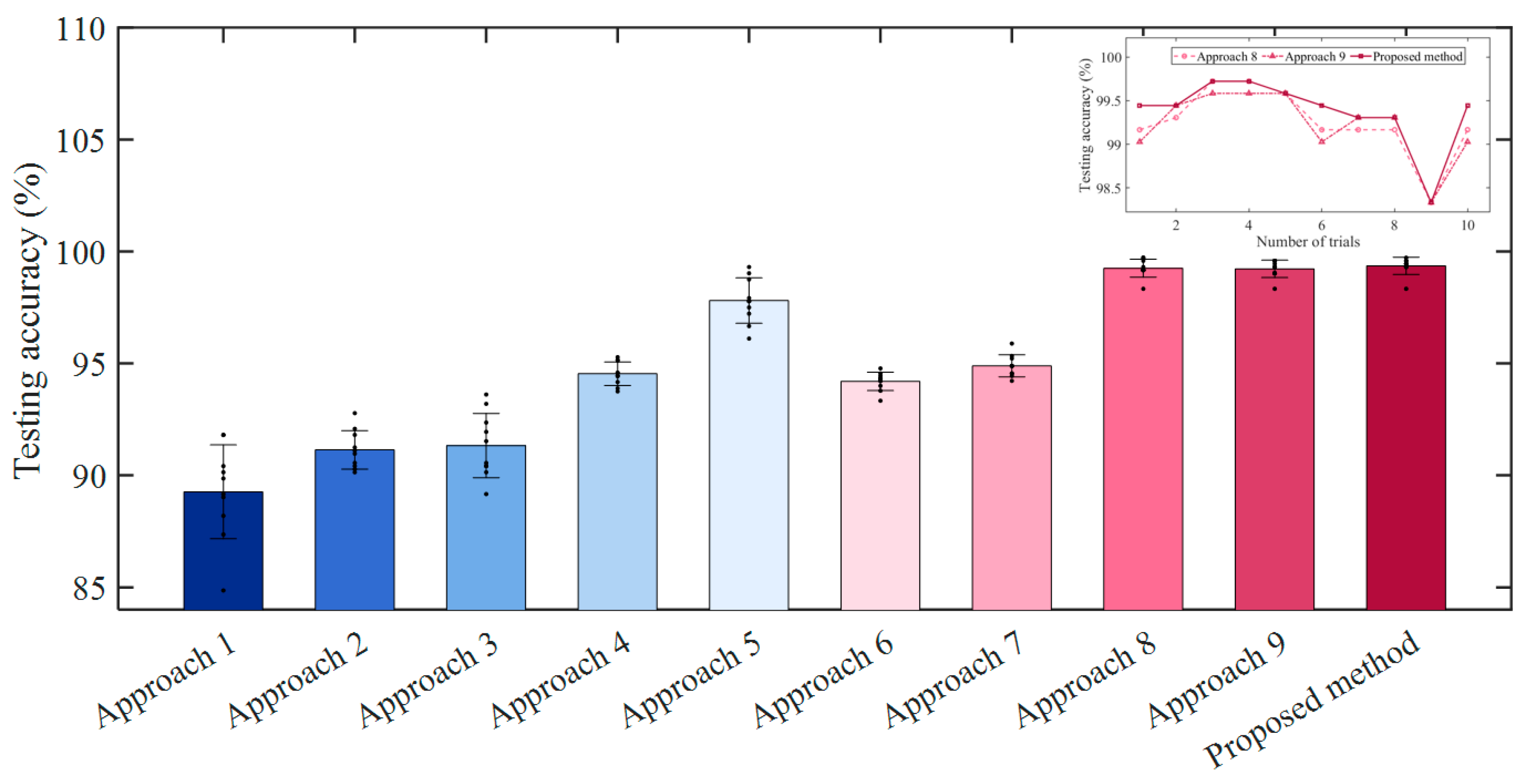
4.4. Comparative Experiments and Results

In order to verify the effectiveness and superiority of the proposed approach, it was compared with other fault diagnosis approaches. There are 9 approaches were compared, specifically:

• Approach 1: A fault diagnosis approach based on the data-level fusion driven by principal component analysis (PCA) and CNN. Fuse the signals of all channels by PCA. And input the fusion result into CNN for classification.
• Approach 2: A fault diagnosis approach based on the data-level fusion driven by PCA and VBICNN. Input the fused signals of Approach 1 into VBICNN for classification.
• Approach 3: A fault diagnosis approach based on the data-level fusion driven by linear weighting and CNN. Fuse the signals of all channels by a similarity-based linear weighting method. And input the fusion result into CNN for classification.
• Approach 4: A fault diagnosis approach based on the data-level fusion driven by linear weighting and VBICNN. Input the fused signals of Approach 3 into VBICNN for classification.
• Approach 5: A diagnosis approach based on statistical feature fusion. Extract the statistical features of the signals of each channel. The features of all channels were combined with the Softmax classifier for classification. The statistical features used are consistent with the reference [41].
• Approach 6: A fault diagnosis approach based on the feature-level fusion driven by sparse auto-encoder (SAE). Extract the features of each channel signal by using SAE. The features of all channels were combined with the Softmax classifier for classification.
• Approach 7: A fault diagnosis approach based on the feature-level fusion driven by variational auto-encoder (VAE). Extract the features of each channel signal by using VAE. The features of all channels were combined with the Softmax classifier for classification.
• Approach 8: A decision-level fusion method based on the average voting. Based on the pre-diagnosis results of each channel obtained by VBICNN, use the average voting to assign the weights of each VBICNN for fusion.
• Approach 9: A decision-level fusion method based on weighted voting. Adopt the second fusion strategy proposed in the reference [40] to assign the weights of each VBICNN for fusion.

Ten repeated runs were performed to calculate the average testing accuracy and standard deviation. The results are shown in Figure 8. Approaches 1–9 provided average accuracies of 89.26%, 91.14%, 91.33%, 94.54%, 97.81%, 94.20%, 94.89%, 99.25%, 99.22%, with standard deviations of 2.0972, 0.8601, 1.4347, 0.5243, 1.0139, 0.4118, in order, 0.4914, 0.3993, and 0.3884. The average accuracy of the proposed method was 99.36% with a standard deviation of 0.3829, which shows that the proposed method is more accurate and reliable.

5. Discussion

5.1. The Necessity of Multi-Channel Information Fusion Diagnosis

A randomly selected set of results from the ablation experiments was used to calculate the confusion matrix for VBICNN. The results are shown in Figure 9, where the horizontal and vertical axes are the predicted and true labels, respectively. As can be seen from the figure, the signals from different channels have different diagnosis accuracies for each fault type. For instance, channel 1 is excellent at recognizing fault types 2, 5, 6, and 8, with 100% diagnostic accuracy, and there is underreporting of other fault types. Channel 2 recognizes fault type 4 with 100% accuracy but is unable to recognize other fault types with 100% accuracy. Channel 3 can diagnose all verification samples for fault types 5 and 9, but there are omissions for other fault types. In parallel, Figure 9 also reflects that the information of each channel signal is complementary. For instance, Channel 1 and Channel 2 appear to be unable to identify fault type 9, whereas Channel 3 makes a significant contribution. Channel 3 has a low accuracy for type 4, but this can be corrected by sensor 2. This phenomenon occurs because the signals from different channels carry different information about the bearing. Reviewing the multi-channel signals introduced in Section 4.1, channels 1–3 collected vibration data in three orthogonal directions on the bearing surface. The existing analysis results of the bearing dynamic response show that there are differences in the vibration response in different directions [42,43]. Thus, the multi-channel vibration signals carry different information, resulting in differences in diagnosis accuracy. Meanwhile, research on the behavioral analysis of high-speed bearing-rotor systems has shown that two orthogonal vibration signals, within the same cross-section, exhibit steady-state eddy characteristics when the system is in smooth operation [44]. So, the mutually orthogonal signals used in the experimental case are closely correlated, which makes the multi-channel diagnosis results complementary. Based on the above, the fusion of information from channels 1–3 is beneficial in guaranteeing the accuracy and reliability of the diagnosis results. According to the results of the ablation experiments, the optimal diagnostic accuracy and average accuracy of VBICNN with a single channel are 98.61% and 97.38%, respectively, and those of the proposed method are 99.72% and 99.36%, which shows that the fusion of multi-channels improves the accuracy of diagnosis.

5.2. The Effectiveness of Variational Bayesian Inference

Comparing the model containing variational Bayesian inference and the model without variational Bayesian inference. There are five sets of comparison results, namely, CNN and VBICNN with channels 1–3 in the ablation experiment, and CNN and VBICNN with PCA data fusion signals and weighted data fusion signals in the comparison experiment. The comparison results are shown in Figure 10. As can be seen from the figure, the model improved with variational Bayesian inference has a significant advantage in terms of diagnosis accuracy, both in the case of single-channel signals as inputs and multi-channel fusion signals as inputs. At the same time, the results of 10 repeated experiments have less fluctuation.

6. Conclusions

To address the issue of incomplete diagnosis information from a single signal, a new multi-sensor fusion fault diagnosis approach is proposed in this paper. Firstly, a basic diagnosis model based on VBICNN is constructed. Secondly, vibration signals from multiple channels were used to train a series of basic VBICNNs to provide multiple pre-diagnosis results. Then, a voting strategy based on verification accuracy is used to assign weights to each model, obtaining more reliable collaborative diagnostic results. In order to validate the proposed method, ablation experiments, and comparative experiments have been carried out. The following conclusions can be drawn:

(1)

The comparison with the diagnosis method based on a single-channel signal confirmed that multi-channel signals contain complementary information, which enables the acquisition of more accurate and stable results.

(2)

The comparison with the models without variational Bayesian inference confirms that variational Bayesian inference has the advantage of dealing with high-dimensional uncertain data, which could improve the classification performance of CNN.

(3)

Comparison with other multichannel fusion approaches confirms that the proposed approach has better performance in multi-channel vibration signal fusion diagnosis. The comparison approaches include several data-level fusion methods, feature-level fusion methods, and decision-level fusion methods.

Although the proposed method demonstrates excellent performance on experimental data with complex interference, the weighted voting strategy used for information fusion is relatively simple and employs a fixed validation accuracy to determine the weights. To enhance collaboration among multi-channel signals, it is necessary to investigate dynamic fusion strategies to learn the optimal weights during the training process. Therefore, we will explore the dynamic weight assignment strategy of the proposed method in the future. Meanwhile, it should be noted that the proposed method is applicable not only to bearings but also to rotating components such as gears. For other anomaly detection problems, such as the Tennessee Eastman process, the framework of the proposed methodology can also be adopted, but a more appropriate basic diagnosis model needs to be reconstructed according to the specific task.

References

1. Alshorman, O.; Irfan, M.; Abdelrahman, R.B.; Abdelrahman, B.; Masadeh, M.; Alshorman, A.; Sheikh, M.A.; Saad, N.; Rahman, S. Advancements in condition monitoring and fault diagnosis of rotating machinery: A comprehensive review of image-based intelligent techniques for induction motors. Eng. Appl. Artif. Intell. 2024, 130, 107724. [Google Scholar] [CrossRef]
2. Liu, L.; Cheng, Y.; Song, D.; Zhang, W.; Tang, G.; Luo, Y. A lightweight network with adaptive input and adaptive channel pruning strategy for bearing fault diagnosis. IEEE Trans. Instrum. Meas. 2024, 73, 3510911. [Google Scholar] [CrossRef]
3. Peng, D.; Wang, H.; Liu, Z.; Zhang, W.; Zuo, M.; Chen, J. Multibranch and multiscale CNN for fault diagnosis of wheelset bearings under strong noise and variable load condition. IEEE Trans. Ind. Inform. 2017, 16, 4949–4960. [Google Scholar] [CrossRef]
4. Strombergsson, D.; Marklund, P.; Berglund, K.; Larsson, P.E. Bearing monitoring in the wind turbine drivetrain: A comparative study of the FFT and wavelet transforms. Wind Energy 2020, 23, 1380–1393. [Google Scholar] [CrossRef]
5. Sahraoui, M.A.; Rahmoune, C.; Meddour, I.; Bettahar, T.; Zair, M. New criteria for wrapper feature selection to enhance bearing fault classification. Adv. Mech. Eng. 2023, 15, 16878132231183862. [Google Scholar] [CrossRef]
6. Kumar, D.; Mehran, S.; Shaikh, M.Z.; Hussain, M.; Chowdhry, B.S.; Hussain, T. Triaxial bearing vibration dataset of induction motor under varying load conditions. Data Brief 2022, 42, 108315. [Google Scholar] [CrossRef]
7. Chen, B.; Cheng, Y.; Allen, P.; Wang, S.; Gu, F.; Zhang, W.; Ball, A.D. A product envelope spectrum generated from spectral correlation/coherence for railway axle-box bearing fault diagnosis. Mech. Syst. Signal Proc. 2025, 225, 112262. [Google Scholar] [CrossRef]
8. Igba, J.; Alemzadeh, K.; Durugbo, C.; Eiriksson, E.T. Analysing RMS and peak values of vibration signals for condition monitoring of wind turbine gearboxes. Renew. Energy 2016, 91, 90–106. [Google Scholar] [CrossRef]
9. Li, Y.; Zhang, W.; Xiong, Q.; Lu, T.; Mei, G. A novel fault diagnosis model for bearing of railway vehicles using vibration signals based on symmetric alpha-stable distribution feature extraction. Shock Vib. 2016, 2016, 5714195. [Google Scholar] [CrossRef]
10. Chen, B.; Song, D.; Zhang, W.; Cheng, Y. A novel spectral coherence-based envelope spectrum for railway axle-box bearing damage identification. Struct. Health Monit. 2023, 22, 879–896. [Google Scholar] [CrossRef]
11. Hou, H.; Zhang, X.; Wang, X.; Wan, Y.; Shi, H.; Liu, W.; Wang, P. Location of underground multilayer media based on BP neural network and near-field electromagnetic signal. IEEE Sens. J. 2025, 25, 725–736. [Google Scholar] [CrossRef]
12. Wang, X.; Jiang, H. Gearbox fault diagnosis based on refined time-shift multiscale reverse dispersion entropy and optimised support vector machine. Machines 2023, 11, 646. [Google Scholar] [CrossRef]
13. Ziani, R.; Felkaoui, A.; Zegadi, R. Bearing fault diagnosis using multiclass support vector machines with binary particle swarm optimization and regularized Fisher’s criterion. J. Intell. Manuf. 2017, 28, 405–417. [Google Scholar] [CrossRef]
14. Yao, C.; Li, N.; Feng, Z.; Chen, D. Fault diagnosis based on rough set attribute reduction and bayesian classifier. China Mech. Eng. 2015, 26, 1969–1977. [Google Scholar]
15. Dong, S.; Wang, P.; Abbas, K. A survey on deep learning and its applications. Comput. Sci. Rev. 2021, 40, 100379. [Google Scholar] [CrossRef]
16. LeCun, Y.; Bengio, Y.; Hinton, G. Deep learning. Nature 2015, 521, 436–444. [Google Scholar] [CrossRef]
17. Janssens, O.; Slavkovikj, V.; Vervisch, B.; Stockman, K.; Loccufier, M.; Verstockt, S.; Van de Wallk, R.; Van Hoecke, S. Convolutional neural network based fault detection for rotating machinery. J. Sound Vibr. 2016, 377, 331–345. [Google Scholar] [CrossRef]
18. Zhang, J.; Yang, Z.; Chen, X.; Zhai, Z.; Liu, Y. Interpretability discussion on convolutional neural network in bearing fault diagnosis. Bearing 2020, 7, 54–60. [Google Scholar]
19. Mohiuddin, M.; Islam, M.S.; Islam, S.; Miah, M.S.; Niu, M. Intelligent Fault Diagnosis of Rolling Element Bearings Based on Modified AlexNet. Sensors 2023, 23, 7764. [Google Scholar] [CrossRef]
20. Ruan, D.; Wang, J.; Yan, J.; Gühmann, C. CNN parameter design based on fault signal analysis and its application in bearing fault diagnosis. Adv. Eng. Inform. 2023, 55, 101877. [Google Scholar] [CrossRef]
21. Salunkhe, V.G.; Khot, S.M.; Jadhav, P.S.; Yelve, N.P.; Kumbhar, M.B. Experimental Investigation Using Robust Deep VMD-ICA and 1D-CNN for Condition Monitoring of Roller Element Bearing. J. Comput. Inf. Sci. Eng. 2024, 24, 124501. [Google Scholar] [CrossRef]
22. Xu, Y.; Feng, K.; Yan, X.; Sheng, X.; Sun, B.; Liu, Z.; Yan, R. Cross-modal fusion convolutional neural networks with online soft-label training strategy for mechanical fault diagnosis. IEEE Trans. Ind. Inform. 2024, 20, 73–84. [Google Scholar] [CrossRef]
23. Yang, S.; Wang, Y.; Li, C. Wind turbine gearbox fault diagnosis based on an improved supervised autoencoder using vibration and motor current signals. Meas. Sci. Technol. 2021, 32, 114003. [Google Scholar] [CrossRef]
24. Xie, T.; Huang, X.; Choi, S. Intelligent mechanical fault diagnosis using multisensor fusion and convolution neural network. IEEE Trans. Ind. Inform. 2022, 18, 3213–3223. [Google Scholar] [CrossRef]
25. Chen, X.; Shao, H.; Xiao, Y.; Yan, S.; Cai, B.; Liu, B. Collaborative fault diagnosis of rotating machinery via dual adversarial guided unsupervised multi-domain adaptation network. Mech. Syst. Signal Proc. 2023, 198, 119427. [Google Scholar] [CrossRef]
26. Stief, A.; Ottewill, J.; Baranowski, J.; Orkisz, M. A PCA and two-stage bayesian sensor fusion approach for diagnosing electrical and mechanical faults in induction motors. IEEE Trans. Ind. Electron. 2019, 66, 9510–9520. [Google Scholar] [CrossRef]
27. Wang, C.; Xin, C.; Xu, Z.; Qin, M.; He, M. Mix-VAEs: A novel multisensor information fusion model for intelligent fault diagnosis. Neurocomputing 2022, 492, 234–244. [Google Scholar] [CrossRef]
28. Mejbel, B.G.; Sarow, S.A.; Al-Sharify, M.T.; Al-Haddad, L.A.; Ogaili, A.A.F.; Al-Sharify, Z.T. A Data Fusion Analysis and Random Forest Learning for Enhanced Control and Failure Diagnosis in Rotating Machinery. J. Fail. Anal. Prev. 2024, 24, 2979–2989. [Google Scholar] [CrossRef]
29. Huo, Z.; Martinez-Garcia, M.; Zhang, Y.; Shu, L. A Multisensor Information Fusion Method for High-Reliability Fault Diagnosis of Rotating Machinery. IEEE Trans. Instrum. Meas. 2022, 71, 3500421. [Google Scholar] [CrossRef]
30. Li, X.; Jiang, H.; Niu, M.; Wang, R. An enhanced selective ensemble deep learning method for rolling bearing fault diagnosis with beetle antennae search algorithm. Mech. Syst. Signal Proc. 2020, 142, 106752. [Google Scholar] [CrossRef]
31. Xu, X.; Song, D.; Wang, Z.; Zheng, Z. A novel collaborative bearing fault diagnosis method based on multisignal decision-level dynamically enhanced fusion. IEEE Sens. J. 2024, 24, 34766. [Google Scholar] [CrossRef]
32. Lecun, Y.; Bottou, L.; Bengio, Y.; Haffner, P. Gradient-based learning applied to document recognition. Proc. IEEE 1998, 86, 2278–2324. [Google Scholar] [CrossRef]
33. Zhao, X.; Wang, L.; Zhang, Y.; Han, X.; Deveci, M.; Parmar, M. A review of convolutional neural networks in computer vision. Artif. Intell. Rev. 2024, 57, 99. [Google Scholar] [CrossRef]
34. Yasin, M.; Sarigül, M.; Avci, M. Logarithmic Learning Differential Convolutional Neural Network. Neural Netw. 2024, 172, 106114. [Google Scholar] [CrossRef]
35. Momeny, M.; Latif, A.M.; Sarram, M.A.; Sheikhpour, R.; Zhang, Y. A noise robust convolutional neural network for image classification. Results Eng. 2021, 10, 100225. [Google Scholar] [CrossRef]
36. Fox, C.; Roberts, S. A tutorial on variational Bayesian inference. Artif. Intell. Rev. 2012, 38, 85–95. [Google Scholar] [CrossRef]
37. Zhang, C.; Bütepage, J.; Kjellström, H.; Mandt, S. Advances in Variational Inference. IEEE Trans. Pattern Anal. Mach. Intell. 2019, 41, 2008–2026. [Google Scholar] [CrossRef]
38. Cao, Y.; Jan, N.M.; Huang, B.; Wang, Y.; Pan, Z.; Gui, W. No-delay multimodal process monitoring using Kullback-Leibler divergence-based statistics in probabilistic mixture models. IEEE Trans. Autom. Sci. Eng. 2023, 20, 167–178. [Google Scholar] [CrossRef]
39. Lin, H.; Hu, C. Variational inference based distributed noise adaptive Bayesian filter. Signal Process. 2021, 178, 107775. [Google Scholar] [CrossRef]
40. Chao, Q.; Gao, H.; Tao, J.; Wang, Y.; Zhou, J.; Liu, C. Adaptive decision-level fusion strategy for the fault diagnosis of axial piston pumps using multiple channels of vibration signals. Sci. China-Technol. Sci. 2022, 65, 470–480. [Google Scholar] [CrossRef]
41. Chen, Z.; Li, W. Multisensor feature fusion for bearing fault diagnosis using sparse autoencoder and deep belief network. IEEE Trans. Instrum. Meas. 2017, 66, 1693–1702. [Google Scholar] [CrossRef]
42. Ohta, H.; Sugimoto, N. Vibration characteristics of tapered roller bearings. J. Sound Vibr. 1996, 190, 137–147. [Google Scholar] [CrossRef]
43. Li, N.; Zhang, J.; Meng, X.; Han, Q.; Zhai, J. Dynamic response and failure analysis of bearing under the impact of vibration excitation. Eng. Fail. Anal. 2023, 154, 107640. [Google Scholar] [CrossRef]
44. Zhang, J.; Han, D.; Xie, Z.; Huang, C.; Rao, Z.; Song, M.; Su, Z. Nonlinear behaviors analysis of high-speed rotor system supported by aerostatic bearings. Tribol. Int. 2022, 170, 107111. [Google Scholar] [CrossRef]
Figure 1. Structure of CNN.
Machines 13 00216 g001
Figure 2. Framework of the proposed bearing fault diagnosis model. Where the red boxes represent the segments intercepted from the raw signals as inputs to the model.
Machines 13 00216 g002
Figure 3. Schematic diagram of the models: (a) CNN; (b) VBICNN. Where nx is the number of neurons in the flattened layer, nz is the number of neurons in the fully connected layer in the CNN, nF is the number of features extracted by the VBICNN, nz is equal to nF, and the red boxes represent the segments intercepted from the raw signals as inputs to the model.
Machines 13 00216 g003
Figure 4. Framework and main steps of the proposed method.
Machines 13 00216 g004
Figure 5. Test-bed for axlebox bearing of high-speed train.
Machines 13 00216 g005
Figure 6. Five kinds of fault bearings.
Machines 13 00216 g006
Figure 7. Results of repeated diagnostics using different channel signals for different fault diagnostic models (horizontal axis is the number of runs, vertical axis is the test accuracy): (a) CNN by channel 1; (b) VBCNN by channel 1; (c) CNN by channel 2; (d) VBCNN by channel 2; (e) CNN by channel 3; (f) VBCNN by channel 3; (g) proposed method using all channels; (h) comparison of results, where different colors represent different models using different channel signals, and the color meanings are consistent with (ag).
Machines 13 00216 g007
Figure 8. Diagnosis results for different approaches.
Machines 13 00216 g008
Figure 9. Confusion matrices of the basic diagnosis mode with different channel signals: (a) Channel 1; (b) Channel 2; (c) Channel 3.
Machines 13 00216 g009
Figure 10. Comparison of diagnostic results.
Machines 13 00216 g010