
Autonomous Agricultural Robot Using YOLOv8 and ByteTrack for Weed Detection and Destruction


Abstract
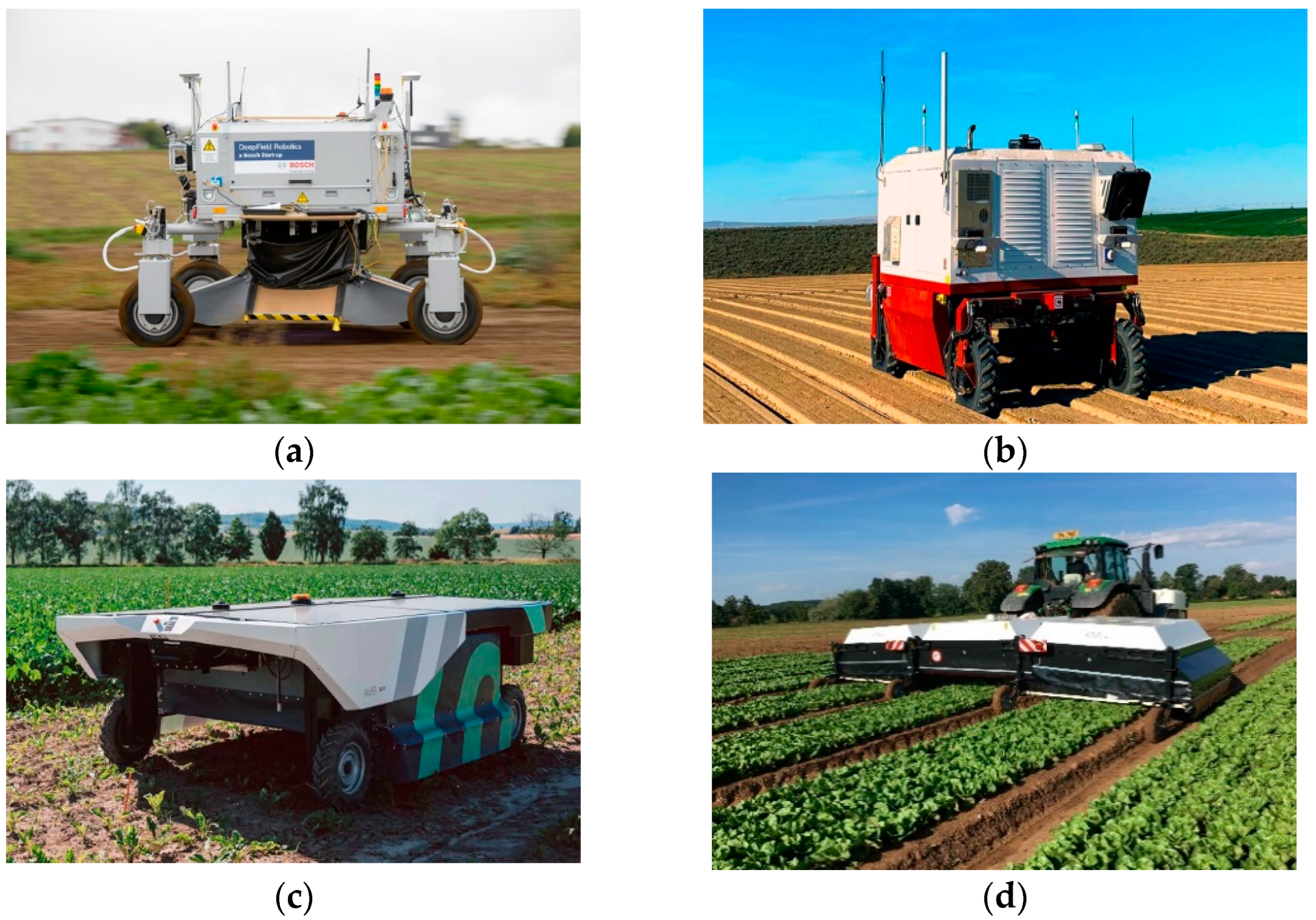
1. Introduction
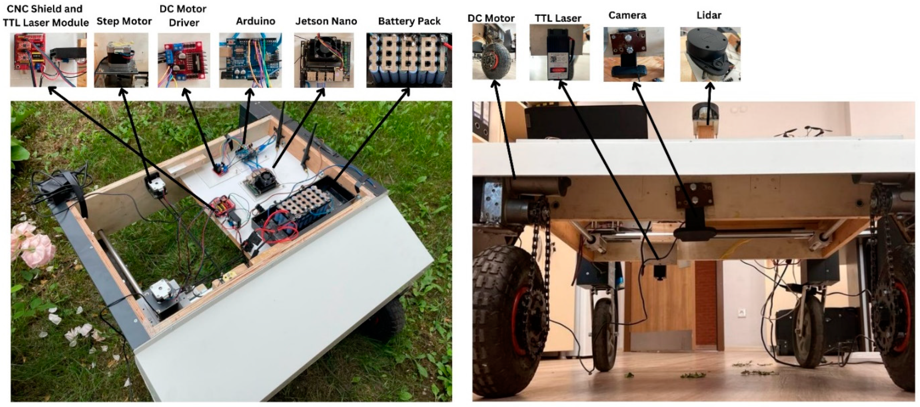
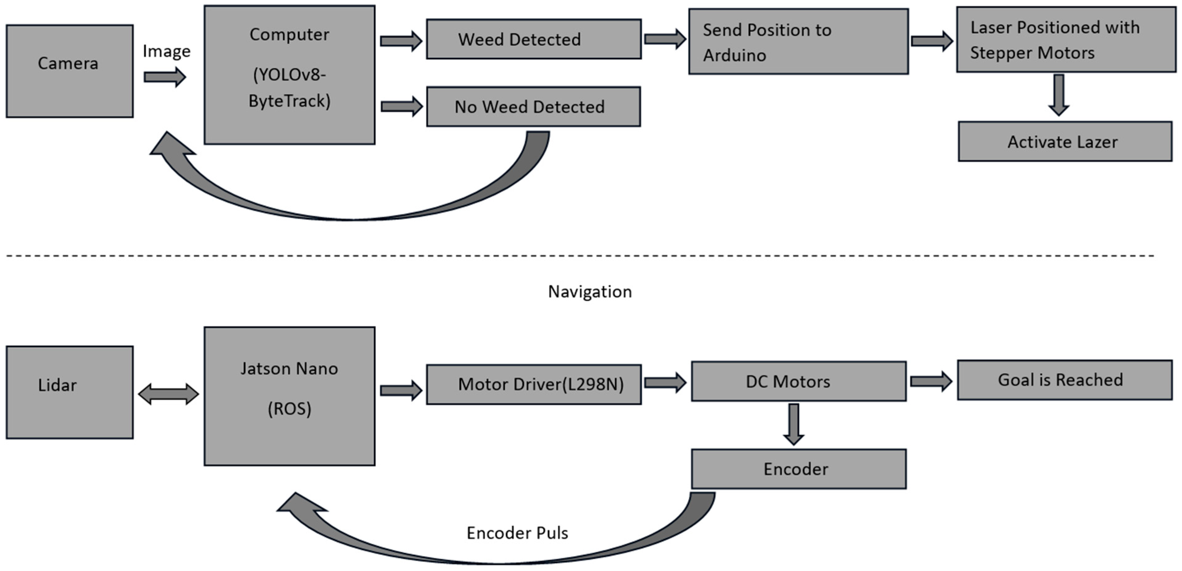
2. Materials and Methods
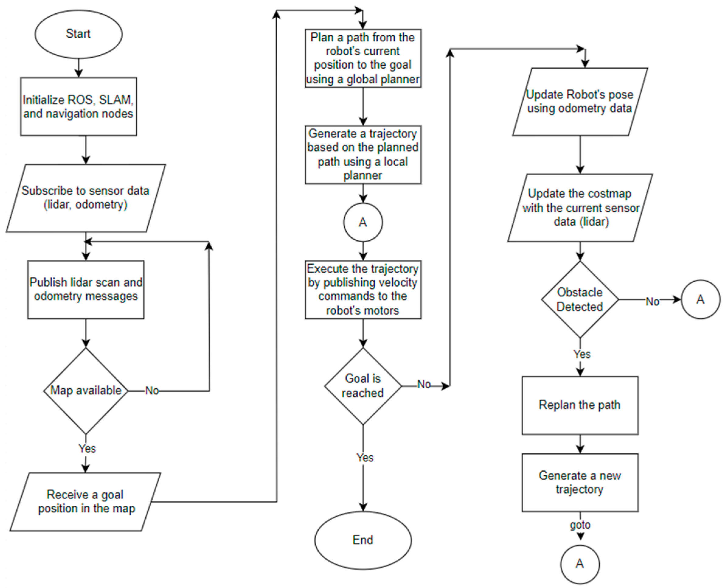
2.1. Autonomous Navigation
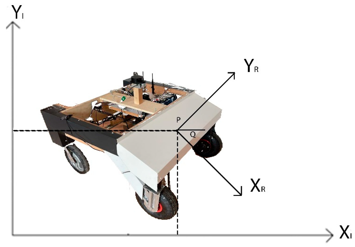
2.1.1. Differential Drive
2.1.2. Localization and Mapping
2.2. Weed Detection and Tracking
2.2.1. YOLO (You Only Look Once)
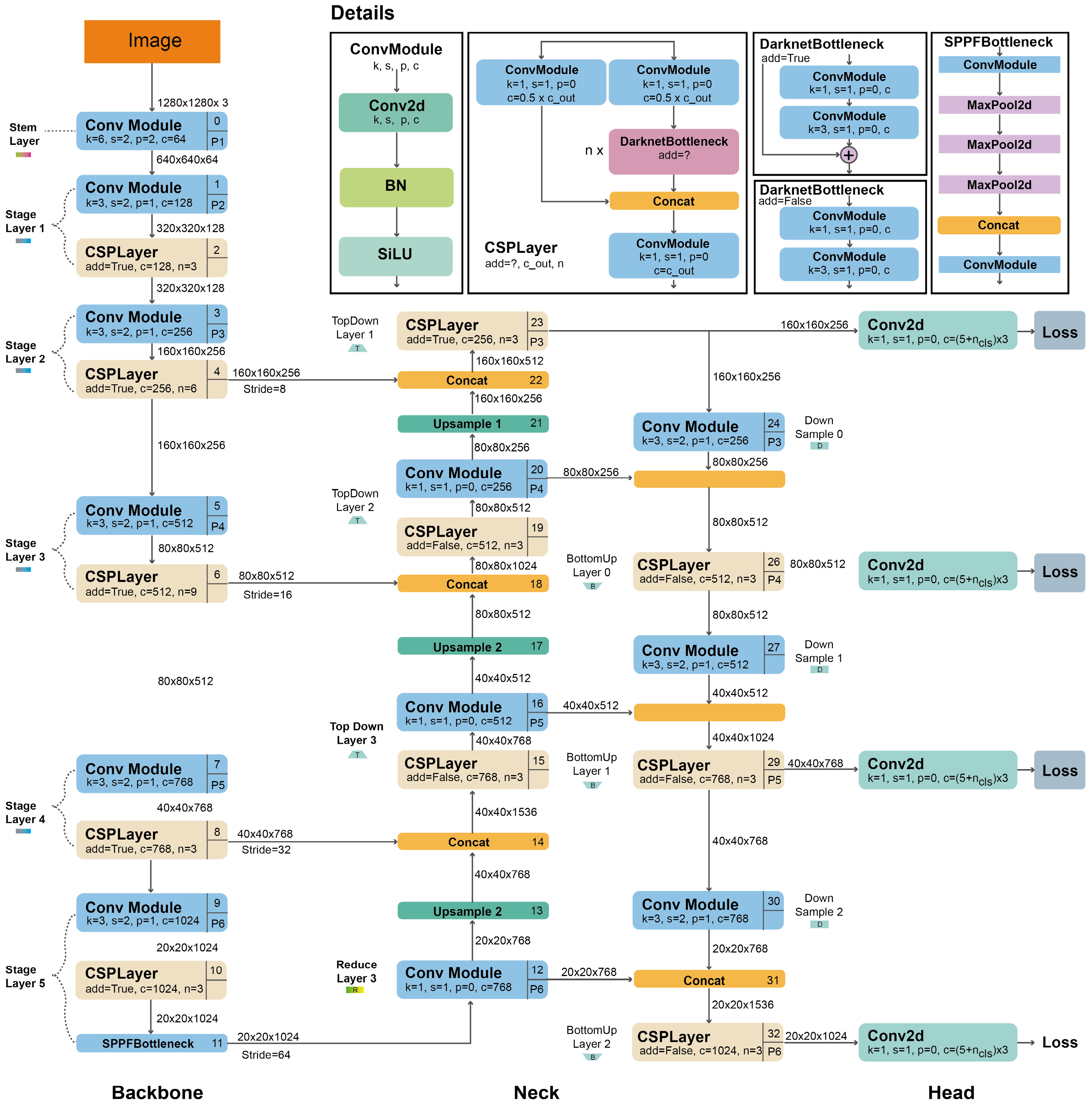
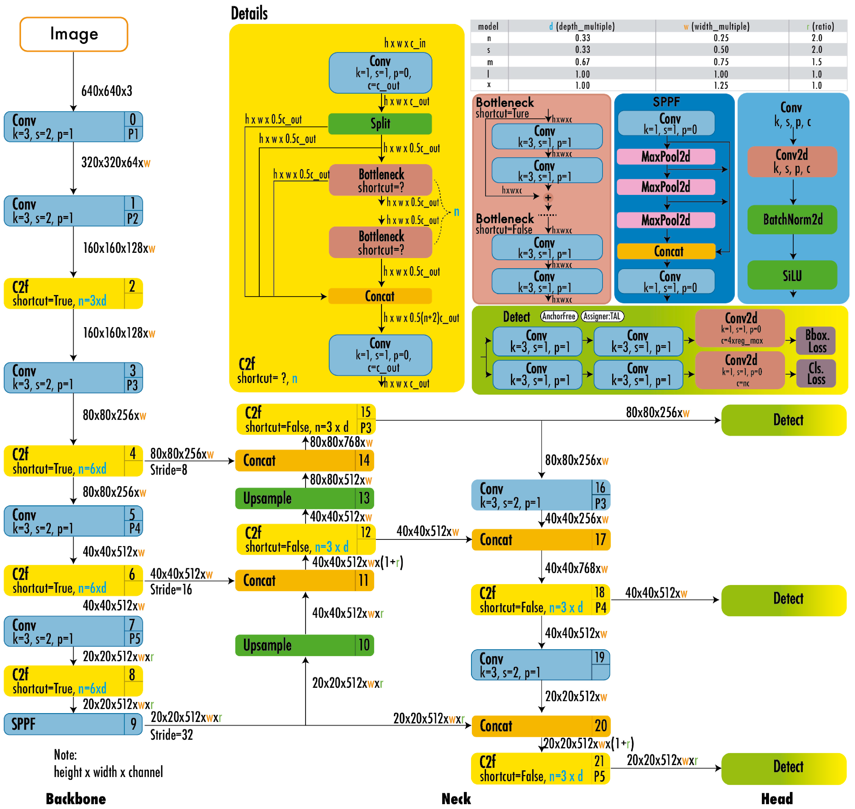
2.2.2. YOLO Models
2.2.3. Pruning and Quantization
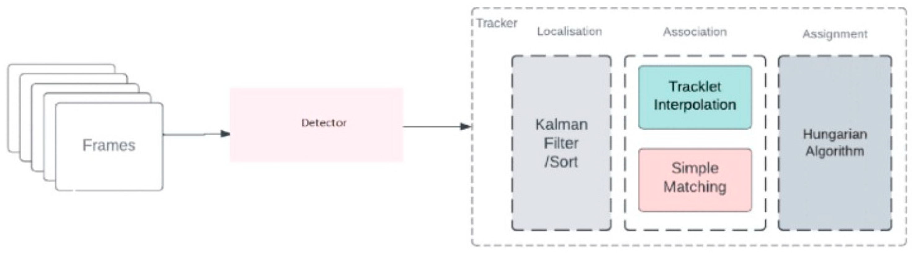
2.2.4. Weed Tracking with ByteTrack
2.3. Metrics
3. Results and Discussion
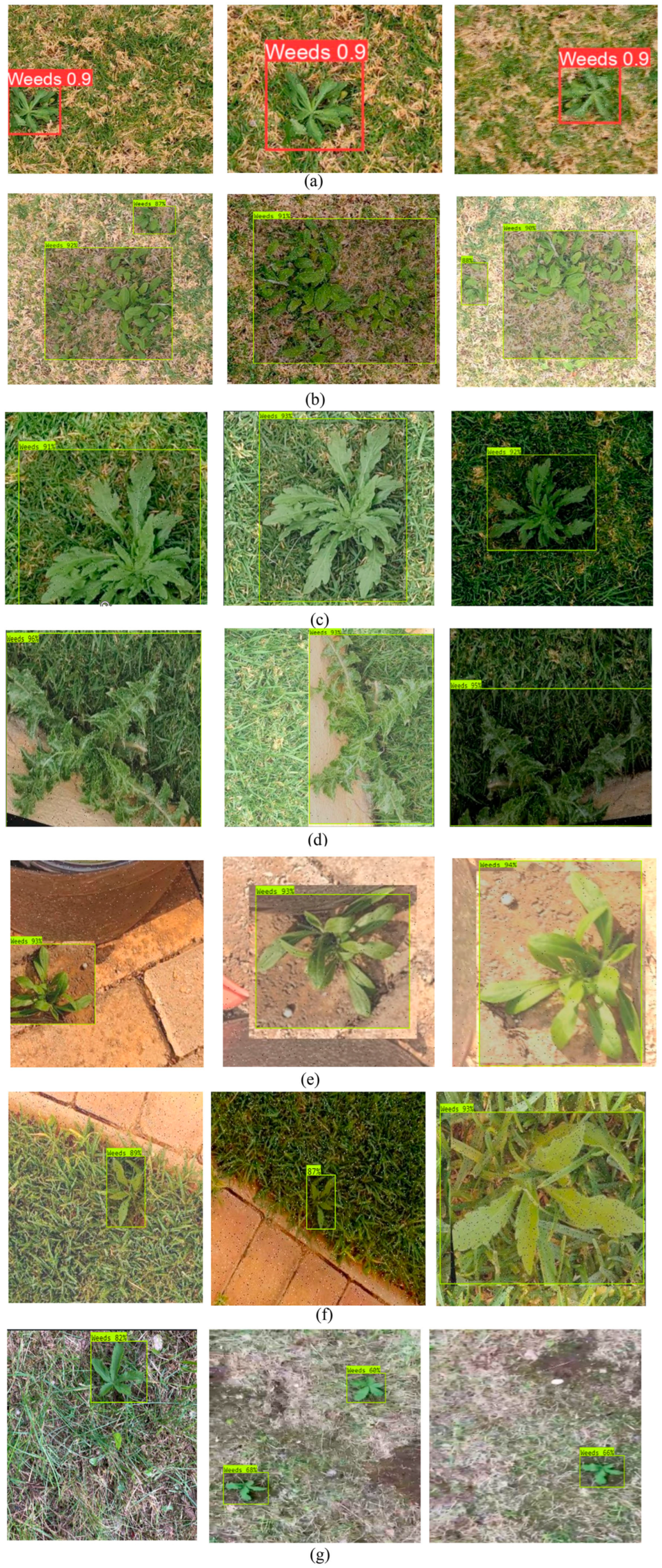
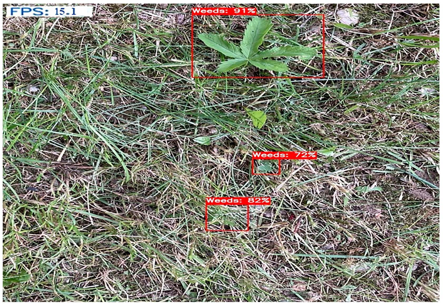
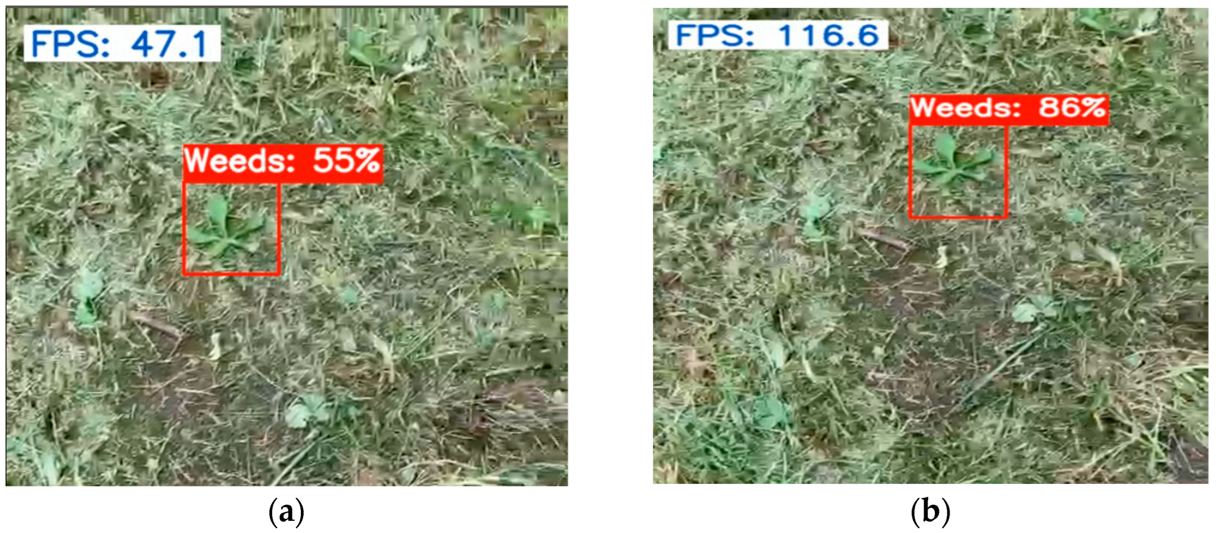
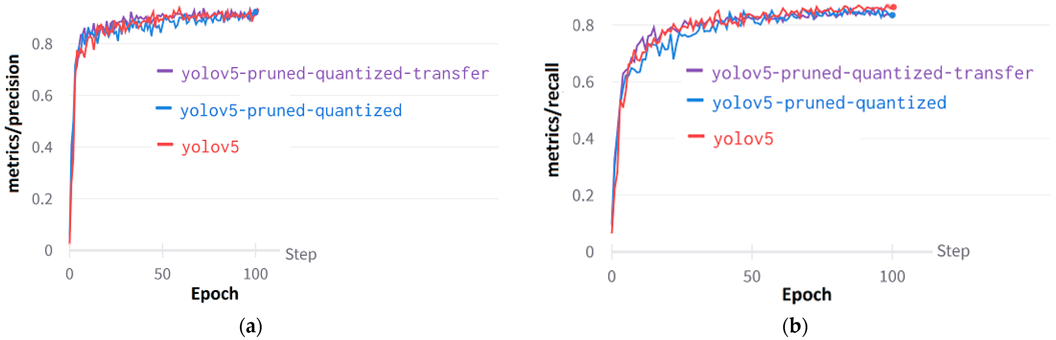
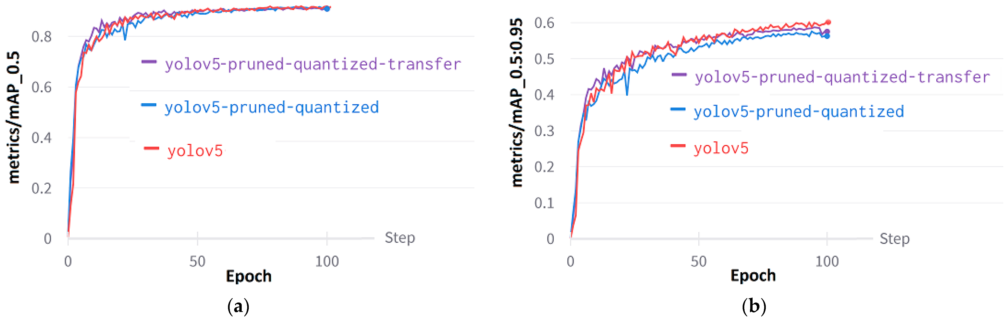
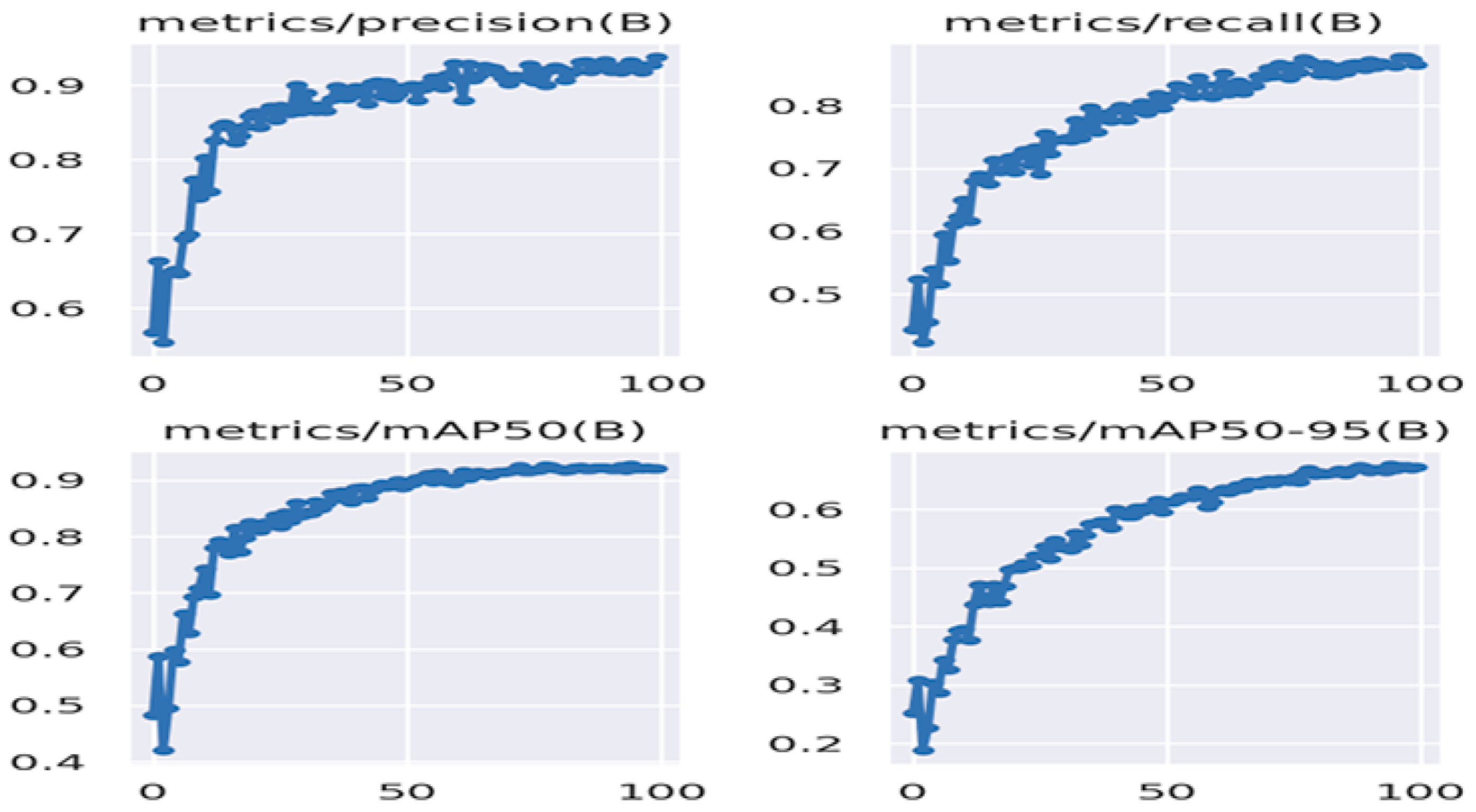
Results of YOLO Models
4. Conclusions
Author Contributions
Funding
Data Availability Statement
Conflicts of Interest
References
- FAO. NSP-Weeds. Available online: http://www.fao.org/agriculture/crops/thematic-sitemap/theme/biodiversity/weeds/en/ (accessed on 8 August 2023).
- Babalola, O.O.; Truter, J.C.; Van Wyk, J.H. Lethal and teratogenic impacts of imazapyr, diquat dibromide, and glufosinate ammonium herbicide formulations using frog embryo teratogenesis assay-xenopus (FETAX). Arch. Environ. Contam. Toxicol. 2021, 80, 708–716. [Google Scholar] [CrossRef] [PubMed]
- Hamuda, E.; Mc Ginley, B.; Glavin, M.; Jones, E. Automatic crop detection under field conditions using the HSV colour space and morphological operations. Comput. Electron. Agric. 2017, 133, 97–107. [Google Scholar] [CrossRef]
- Cho, S.; Lee, D.S.; Jeong, J.Y. AE—Automation and emerging technologies: Weed–plant discrimination by machine vision and artificial neural network. Biosyst. Eng. 2002, 83, 275–280. [Google Scholar] [CrossRef]
- Bakhshipour, A.; Jafari, A.; Nassiri, S.M.; Zare, D. Weed segmentation using texture features extracted from wavelet sub-images. Biosyst. Eng. 2017, 157, 1–12. [Google Scholar] [CrossRef]
- Lottes, P.; Stachniss, C. Semi-supervised online visual crop and weed classification in precision farming exploiting plant arrangement. In Proceedings of the IEEE International Conference on Intelligent Robots and Systems, Vancouver, BC, Canada, 24–28 September 2017; pp. 5155–5161. [Google Scholar] [CrossRef]
- Li, N.; Zhang, X.; Zhang, C.; Ge, L.; He, Y.; Wu, X. Review of machine-vision-based plant detection technologies for robotic weeding. In Proceedings of the 2019 IEEE International Conference on Robotics and Biomimetics (ROBIO), Dali, China, 6–8 December 2019; pp. 2370–2377. [Google Scholar] [CrossRef]
- Hasan, A.M.; Sohel, F.; Diepeveen, D.; Laga, H.; Jones, M.G. A survey of deep learning techniques for weed detection from images. Comput. Electron. Agric. 2021, 184, 106067. [Google Scholar] [CrossRef]
- Rai, N.; Zhang, Y.; Ram, B.G.; Schumacher, L.; Yellavajjala, R.K.; Bajwa, S.; Sun, X. Applications of deep learning in precision weed management: A review. Comput. Electron. Agric. 2023, 206, 107698. [Google Scholar] [CrossRef]
- Bakhshipour, A.; Jafari, A. Evaluation of support vector machine and artificial neural networks in weed detection using shape features. Comput. Electron. Agric. 2018, 145, 153–160. [Google Scholar] [CrossRef]
- Islam, N.; Rashid, M.M.; Wibowo, S.; Xu, C.Y.; Morshed, A.; Wasimi, S.A.; Rahman, S.M. Early weed detection using image processing and machine learning techniques in an Australian chilli farm. Agriculture 2021, 11, 387. [Google Scholar] [CrossRef]
- Haug, S.; Michaels, A.; Biber, P.; Ostermann, J. Plant classification system for crop/weed discrimination without segmentation. In Proceedings of the IEEE Winter Conference on Applications of Computer Vision, Steamboat Springs, CO, USA, 24–26 March 2014; pp. 1142–1149. [Google Scholar] [CrossRef]
- Rahman, A.; Lu, Y.; Wang, H. Performance evaluation of deep learning object detectors for weed detection for cotton. Smart Agric. Technol. 2023, 3, 100126. [Google Scholar] [CrossRef]
- Hu, K.; Wang, Z.; Coleman, G.; Bender, A.; Yao, T.; Zeng, S.; Walsh, M. Deep Learning Techniques for In-Crop Weed Identification: A Review. arXiv 2021, arXiv:2103.14872. Available online: http://xxx.lanl.gov/abs/2103.14872 (accessed on 12 March 2023).
- Hu, K.; Coleman, G.; Zeng, S.; Wang, Z.; Walsh, M. Graph weeds net: A graph-based deep learning method for weed recognition. Comput. Electron. Agric. 2020, 174, 105520. [Google Scholar] [CrossRef]
- Yu, J.; Sharpe, S.M.; Schumann, A.W.; Boyd, N.S. Deep learning for image-based weed detection in turfgrass. Eur. J. Agron. 2019, 104, 78–84. [Google Scholar] [CrossRef]
- Hussain, N.; Farooque, A.A.; Schumann, A.W.; McKenzie-Gopsill, A.; Esau, T.; Abbas, F.; Zaman, Q. Design and development of a smart variable rate sprayer using deep learning. Remote Sens. 2020, 12, 4091. [Google Scholar] [CrossRef]
- Ruigrok, T.; van Henten, E.; Booij, J.; van Boheemen, K.; Kootstra, G. Application-specific evaluation of a weed-detection algorithm for plant-specific spraying. Sensors 2020, 20, 7262. [Google Scholar] [CrossRef]
- Junior, L.C.M.; Ulson, C.A.J. Real time weed detection using computer vision and deep learning. In Proceedings of the 14th IEEE International Conference on Industry Applications (INDUSCON), São Paulo, Brazil, 15–18 August 2021; pp. 1131–1137. [Google Scholar] [CrossRef]
- Rehman, M.U.; Eesaar, H.; Abbas, Z.; Seneviratne, L.; Hussain, I.; Chong, K.T. Advanced drone-based weed detection using feature-enriched deep learning approach. Knowl.-Based Syst. 2024, 305, 112655. [Google Scholar] [CrossRef]
- Li, Y.; Guo, Z.; Sun, Y.; Chen, X.; Cao, Y. Weed Detection Algorithms in Rice Fields Based on Improved YOLOv10n. Agriculture 2024, 14, 2066. [Google Scholar] [CrossRef]
- Åstrand, B.; Baerveldt, A.J. An agricultural mobile robot with vision-based perception for mechanical weed control. Auton. Robot. 2002, 13, 21–35. [Google Scholar] [CrossRef]
- Bawden, O.; Kulk, J.; Russell, R.; McCool, C.; English, A.; Dayoub, F.; Perez, T. Robot for weed species plant-specific management. J. Field Robot. 2017, 34, 1179–1199. [Google Scholar] [CrossRef]
- Deepfield Robotics-Bosch. Available online: https://spectrum.ieee.org/bosch-deepfield-robotics-weed-control (accessed on 21 December 2024).
- Ecorobitix-ARA. Available online: https://ecorobotix.com/en/ara/ (accessed on 21 December 2024).
- Ecorobitix-AVO. Available online: https://ecorobotix.com/en/avo/ (accessed on 21 December 2024).
- Carbon Robotics. Available online: https://carbonrobotics.com/ (accessed on 21 December 2024).
- Malu, S.K.; Majumdar, J. Kinematics, localization and control of differential drive mobile robot. Glob. J. Res. Eng. 2014, 14, 1–9. [Google Scholar]
- De Giorgi, C.; De Palma, D.; Parlangeli, G. Online Odometry Calibration for Differential Drive Mobile Robots in Low Traction Conditions with Slippage. Robotics 2023, 13, 7. [Google Scholar] [CrossRef]
- Li, X.; Hu, Y.; Jie, Y.; Zhao, C.; Zhang, Z. Dual-Frequency Lidar for Compressed Sensing 3D Imaging Based on All-Phase Fast Fourier Transform. J. Opt. Photonics Res. 2024, 1, 74–81. [Google Scholar] [CrossRef]
- Hu, K.; Chen, Z.; Kang, H.; Tang, Y. 3D vision technologies for a self-developed structural external crack damage recognition robot. Autom. Constr. 2024, 159, 105262. [Google Scholar] [CrossRef]
- Santos, J.M.; Portugal, D.; Rocha, R.P. An evaluation of 2D SLAM techniques available in robot operating system. In Proceedings of the 2013 IEEE International Symposium on Safety, Security, and Rescue Robotics (SSRR), Linköping, Sweden, 21–26 October 2013; pp. 1–6. [Google Scholar] [CrossRef]
- Adanur, F.; Kabataş, M.; Benli, E. Mapping and Navigation on Rough Surface with LIDAR and IMU. In Proceedings of the 2022 Innovations in Intelligent Systems and Applications Conference (ASYU), Antalya, Turkey, 7–9 September 2022; pp. 1–5. [Google Scholar] [CrossRef]
- Redmon, J.; Divvala, S.; Girshick, R.; Farhadi, A. You Only Look Once: Unified, Real-Time Object Detection. In Proceedings of the 2016 IEEE Conference on Computer Vision and Pattern Recognition (CVPR), Las Vegas, NV, USA, 27–30 June 2016; pp. 779–788. [Google Scholar] [CrossRef]
- Dang, F.; Chen, D.; Lu, Y.; Li, Z. YOLOWeeds: A novel benchmark of YOLO object detectors for multi-class weed detection in cotton production systems. Comput. Electron. Agric. 2023, 205, 107655. [Google Scholar] [CrossRef]
- Ying, B.; Xu, Y.; Zhang, S.; Shi, Y.; Liu, L. Weed Detection in Images of Carrot Fields Based on Improved YOLO V4. Trait. Du Signal 2021, 38, 341–348. [Google Scholar] [CrossRef]
- Sportelli, M.; Apolo-Apolo, O.E.; Fontanelli, M.; Frasconi, C.; Raffaelli, M.; Peruzzi, A.; Perez-Ruiz, M. Evaluation of YOLO Object Detectors for Weed Detection in Different Turfgrass Scenarios. Appl. Sci. 2023, 13, 8502. [Google Scholar] [CrossRef]
- Redmon, J.; Farhadi, A. Yolo9000: Better, faster, stronger. In Proceedings of the IEEE Conference on Computer Vision and Pattern Recognition, Honolulu, HI, USA, 21–26 July 2017; pp. 7263–7271. [Google Scholar] [CrossRef]
- Redmon, J.; Farhadi, A. Yolov3: An incremental improvement. arXiv 2018, arXiv:1804.02767. [Google Scholar]
- Bochkovskiy, A.; Wang, C.Y.; Liao, H.Y.M. Yolov4: Optimal speed and accuracy of object detection. arXiv 2020, arXiv:2004.10934. [Google Scholar]
- Jocher, G. YOLOv5 by Ultralytics. Available online: https://github.com/ultralytics/yolov5 (accessed on 22 September 2023).
- Li, C.; Li, L.; Jiang, H.; Weng, K.; Geng, Y.; Li, L.; Ke, Z.; Li, Q.; Cheng, M.; Nie, W. Yolov6: A single-stage object detection framework for industrial applications. arXiv 2022, arXiv:2209.02976. [Google Scholar]
- Wang, C.Y.; Bochkovskiy, A.; Liao, H.Y.M. Yolov7: Trainable bag-of-freebies sets new state-of-the-art for real-time object detectors. arXiv 2022, arXiv:2207.02696. [Google Scholar]
- YOLOv8 by Ultralytics. Available online: https://docs.ultralytics.com/ (accessed on 20 December 2023).
- Wang, C.Y.; Yeh, I.H.; Liao, H.Y.M. Yolov9: Learning what you want to learn using programmable gradient information. arXiv 2024, arXiv:2402.13616. [Google Scholar]
- Wang, A.; Chen, H.; Liu, L.; Chen, K.; Lin, Z.; Han, J.; Ding, G. Yolov10: Real-time end-to-end object detection. arXiv 2024, arXiv:2405.14458. [Google Scholar]
- YOLOv11 by Ultralytics. Available online: https://docs.ultralytics.com/tr/models/yolo11/ (accessed on 1 December 2024).
- Tao, J.; Wang, H.; Zhang, X.; Li, X.; Yang, H. An object detection system based on YOLO in traffic scene. In Proceedings of the 2017 6th International Conference on Computer Science and Network Technology (ICCSNT), Dalian, China, 21–22 October 2017; pp. 315–319. [Google Scholar] [CrossRef]
- Terven, J.; Córdova-Esparza, D.M.; Romero-González, J.A. A Comprehensive Review of YOLO Architectures in Computer Vision: From YOLOv1 to YOLOv8 and YOLO-NAS. Mach. Learn. Knowl. Extr. 2023, 5, 1680–1716. [Google Scholar] [CrossRef]
- Wang, Y.; Mariano, V.Y. A Multi Object Tracking Framework Based on YOLOv8s and Bytetrack Algorithm. IEEE Access 2024, 12, 120711–120719. [Google Scholar] [CrossRef]
- You, L.; Chen, Y.; Xiao, C.; Sun, C.; Li, R. Multi-Object Vehicle Detection and Tracking Algorithm Based on Improved YOLOv8 and ByteTrack. Electronics 2024, 13, 3033. [Google Scholar] [CrossRef]
- Abouelyazid, M. Comparative Evaluation of SORT, DeepSORT, and ByteTrack for Multiple Object Tracking in Highway Videos. Int. J. Sustain. Infrastruct. Cities Soc. 2023, 8, 42–52. [Google Scholar]
- Zhang, Y.; Sun, P.; Jiang, Y.; Yu, D.; Weng, F.; Yuan, Z.; Wang, X. Bytetrack: Multi-object tracking by associating every detection box. In European Conference on Computer Vision; Springer: Cham, Switzerland, 2022; pp. 1–21. [Google Scholar] [CrossRef]
- Yang, X.; Bist, R.; Paneru, B.; Chai, L. Monitoring activity index and behaviors of cage-free hens with advanced deep learning technologies. Poult. Sci. 2024, 103, 104193. [Google Scholar] [CrossRef]
- Aadi, F.Z.A.H.; Sadiq, A.; Labd, Z. Comparing Object Tracking Algorithms for Real-Time Applications: Performance Analysis and Implementation Study. In Proceedings of the 2023 10th International Conference on Wireless Networks and Mobile Communications (WINCOM), Istanbul, Turkiye, 26–28 October 2023; pp. 1–5. [Google Scholar] [CrossRef]
- Chen, J.; Wang, H.; Zhang, H.; Luo, T.; Wei, D.; Long, T.; Wang, Z. Weed detection in sesame fields using a YOLO model with an enhanced attention mechanism and feature fusion. Comput. Electron. Agric. 2022, 202, 107412. [Google Scholar] [CrossRef]
- Roboflow Weeds Dataset. Available online: https://universe.roboflow.com/roboflow-demo-projects/agriculture-328r8/dataset/6 (accessed on 2 May 2024).
- Saleem, M.H.; Potgieter, J.; Arif, K.M. Weed detection by faster RCNN model: An enhanced anchor box approach. Agronomy 2022, 12, 1580. [Google Scholar] [CrossRef]
- Peng, H.; Li, Z.; Zhou, Z.; Shao, Y. Weed detection in paddy field using an improved RetinaNet network. Comput. Electron. Agric. 2022, 199, 107179. [Google Scholar] [CrossRef]

| Model | mAP | Precision | Recall | Fps |
|---|---|---|---|---|
| YOLOv5 | 0.930 | 0.938 | 0.884 | 15 |
| YOLOv5 Pruned and Quan. with Tf. | 0.909 | 0.921 | 0.834 | 47 |
| YOLOv5 Pruned and Quan. | 0.909 | 0.924 | 0.835 | 116 |
| YOLOv8 ByteTrack | 0.921 | 0.938 | 0.865 | 18 |
| YOLOv9 | 0.893 | 0.905 | 0.803 | 21 |
| YOLOv11 | 0.926 | 0.915 | 0.870 | 24 |
Disclaimer/Publisher’s Note: The statements, opinions and data contained in all publications are solely those of the individual author(s) and contributor(s) and not of MDPI and/or the editor(s). MDPI and/or the editor(s) disclaim responsibility for any injury to people or property resulting from any ideas, methods, instructions or products referred to in the content. |
© 2025 by the authors. Licensee MDPI, Basel, Switzerland. This article is an open access article distributed under the terms and conditions of the Creative Commons Attribution (CC BY) license (https://creativecommons.org/licenses/by/4.0/).
Share and Cite
Bajraktari, A.; Toylan, H. Autonomous Agricultural Robot Using YOLOv8 and ByteTrack for Weed Detection and Destruction. Machines 2025, 13, 219. https://doi.org/10.3390/machines13030219
Bajraktari A, Toylan H. Autonomous Agricultural Robot Using YOLOv8 and ByteTrack for Weed Detection and Destruction. Machines. 2025; 13(3):219. https://doi.org/10.3390/machines13030219
Chicago/Turabian StyleBajraktari, Ardin, and Hayrettin Toylan. 2025. "Autonomous Agricultural Robot Using YOLOv8 and ByteTrack for Weed Detection and Destruction" Machines 13, no. 3: 219. https://doi.org/10.3390/machines13030219
APA StyleBajraktari, A., & Toylan, H. (2025). Autonomous Agricultural Robot Using YOLOv8 and ByteTrack for Weed Detection and Destruction. Machines, 13(3), 219. https://doi.org/10.3390/machines13030219