Virtual Prototyping of a Novel Manipulator for Efficient Laser Processing of Complex Large Parts

Abstract

Traditional industrial robots offer significant operational flexibility and adapt well to reconfigurable production systems, although they face limitations in applications demanding high motion performance and spatial positional accuracy. While novel manufacturing solutions supporting small batch productions of custom products are widely researched, they are not yet fully available at industrial level. With the aim to advance in this domain, the present work, conducted in the context of the EU project OPeraTIC, reports the development of a novel manipulator for advanced three-dimensional laser surface treatment of large industrial components. The proposed robotic platform presents a decoupled kinematic architecture, with direct drive actuation in all axes. Its open control ensures adaptability to diverse manufacturing scenarios, making it a versatile tool for modern production lines. Starting from the description of its embodiment design and mechanical layout, the paper delves into robot virtual prototyping focusing on kinematic and dynamics aspects. In particular, a detailed behavioral model covering direct and inverse kinematic calculations, also allowing the precise evaluation of all actuation forces/torques, has been developed using analytical approaches. The model is validated with a commercial solver imposing different spatial motions. The generated performance maps illustrate the robot operational capabilities across a range of work scenarios.

1. Introduction

In an era defined by growing demands for customization, waste reduction, and efficient small-batch production, traditional Industrial Robots (IR) face important challenges. These arise primarily from their rigid programming and limited motion accuracy, which often lead to significant downtime for setup and calibration [1]. IR have typically been employed to perform repetitive tasks in stable, predefined environments. Programming in such contexts was relatively fixed and rarely modified, while all delicate poses were manually taught [2]. Moreover, most IR in use today are heavily dependent on proprietary software platforms provided by their manufacturers, with programming restricted to vendor-specific languages [3].

Today’s manufacturing landscape increasingly requires robots to undergo frequent reprogramming and adjustments in response to diverse and small production lots, making control flexibility an essential feature for all types of IR [4]. Closed, proprietary systems present considerable challenges when adapting to these evolving demands. In particular, their maintenance as well as the integration of new functionalities are often constrained [5]. Additionally, connection with external devices, such as sensors and actuators, is frequently restricted (or partially allowed only through expensive software packages), complicating the creation of interconnected systems [6]. The lack of interoperability between platforms further restrains seamless communication and data exchange, both of which are essential for collaborative and adaptive manufacturing processes. Lastly, restricted user access to low-level control layers prevents the implementation of advanced control strategies, negatively impacting system accuracy and hindering the adoption of sophisticated techniques, e.g., aimed at compensating the robot positional errors [7].

In response to these challenges, there is a strong push toward the development of new systems that combine the benefits of IR and Computerized Numerical Control (CNC) machines, while also integrating open (i.e., customizable, fully programmable) controllers [8]. Indeed, open solutions seamlessly integrate the exceptional precision required for specialized tasks with the flexibility needed for quick adjustments, modular integration, and scalability. As a result, open controllers are well-suited to address the dynamic and ever-evolving needs of modern manufacturing, effectively overcoming the limitations of traditional systems [9,10].

During the development of a new machine, virtual prototypes are generally defined within a Computer Aided Design/Engineering (CAD/CAE) environment, or by resorting to analytical approaches to conduct detailed behavioral studies [11]. These are essential during the design phases, where simulations are conducted to optimize performance and guide the selection and dimensioning of actuation modules [12]. They also help identify critical conditions, such as singularities or unreachable points, to ensure the system meets specifications before physical prototyping and testing [13]. In this context, analytical models are always desirable as they address the limitations of traditional CAE tools, which are often time-consuming when simulating a wide range of operational conditions, e.g., in the case of large parametric studies. Once the design phase is complete, well defined analytical models are also integrated into the controller module to generate motion setpoints and provide feedforward inputs to the servo controller, enhancing control performance and overall operational efficiency [14,15].

Building on these premises, this paper presents a novel manipulator designed for laser surface texturing of 3D components. Its primary scope is to create micro-texturing on surfaces to modify the properties of non-standard parts, which exhibit significant variations in shape and size. The proposed device overcomes the limitations of conventional laser microprocessing, which is typically restricted to flat surfaces, enabling the processing of 3D components. Developed within the EU project OPeraTIC, this machine aims to achieve a competitive advantage in terms of quality, efficiency, emission reduction (by eliminating chemicals and waste), while also enhancing process flexibility and functionality, and motion accuracy during high-dynamics tasks. This study focuses on the mechanical development of the manipulator, providing essential support for both the design phase, including the selection of the kinematic architecture and hardware components, and the subsequent programming of the control system. Through virtual prototyping and dynamic modeling, this work ensures that the system architecture is optimized for accuracy, efficiency, and adaptability to diverse manufacturing needs. The developed analytical model, after validation against a commercial solver, is then used to produce the manipulator performance maps for various working conditions. Additionally, it lays the foundation for the implementation of the OPeraTIC open-architecture controller, which will further enhance process flexibility and customization in industrial applications.

The remainder of the paper is organized as follows. Section 2 presents an overview of the robot design, detailing its mechanical architecture and operational principles. Section 3 and Section 4 focus on the development of the kinematic and dynamic models, respectively, describing the methodologies employed and their relevance to control strategy formulation. Section 5 discusses the validation of the extracted models through simulation (in the RecurDyn environment) and presents performance maps that illustrate the manipulator operational capabilities. Finally, Section 6 reports the concluding remarks.

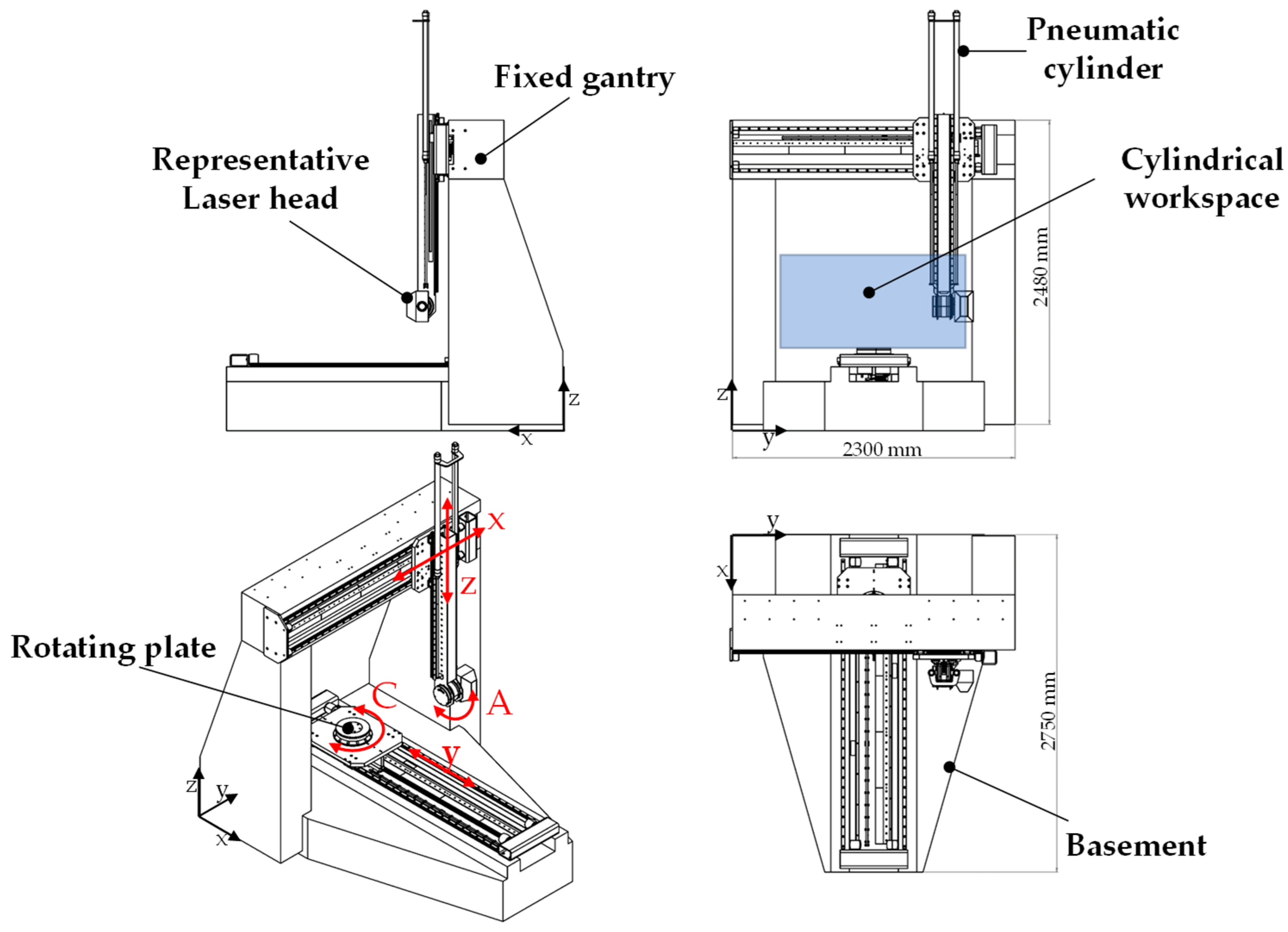
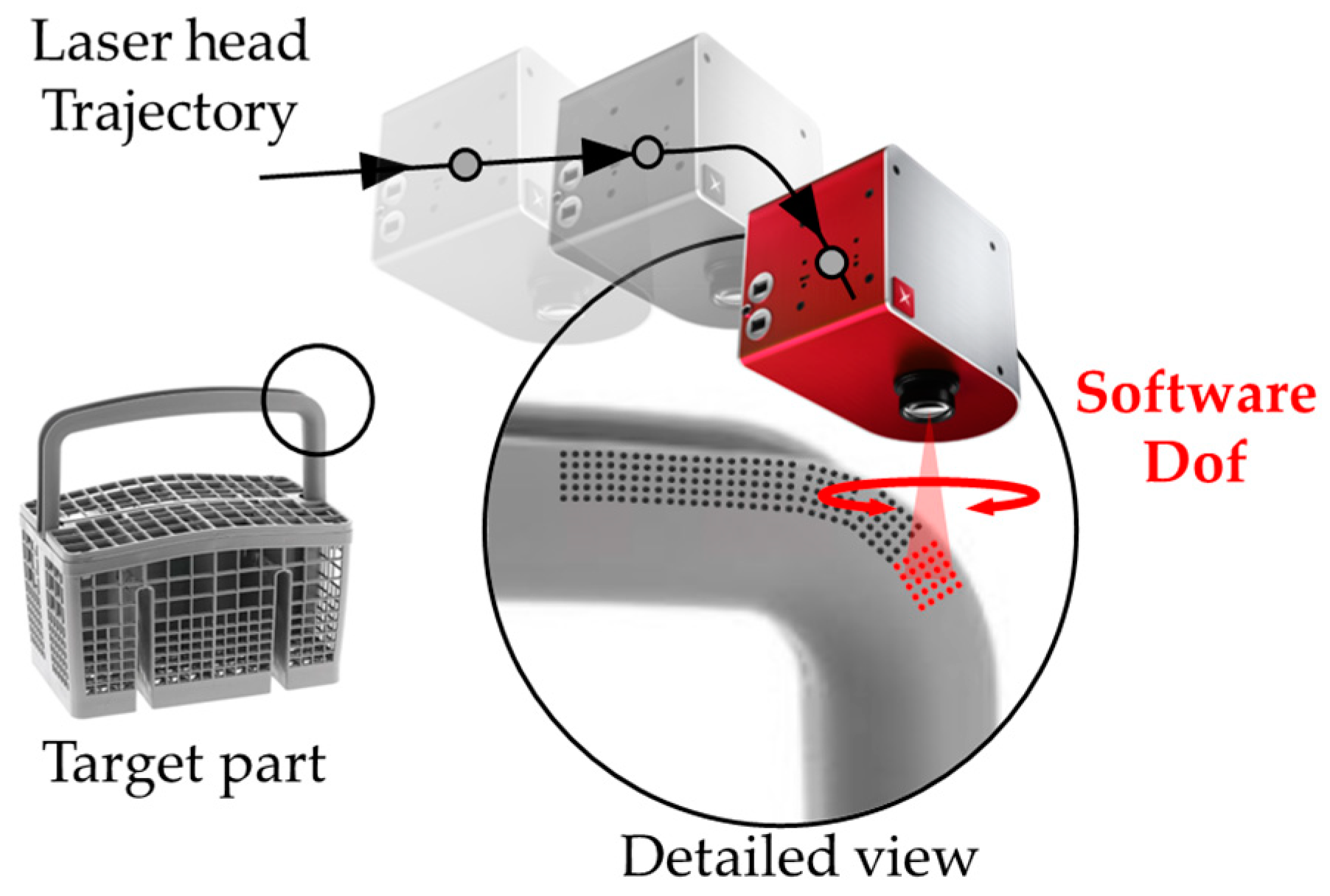
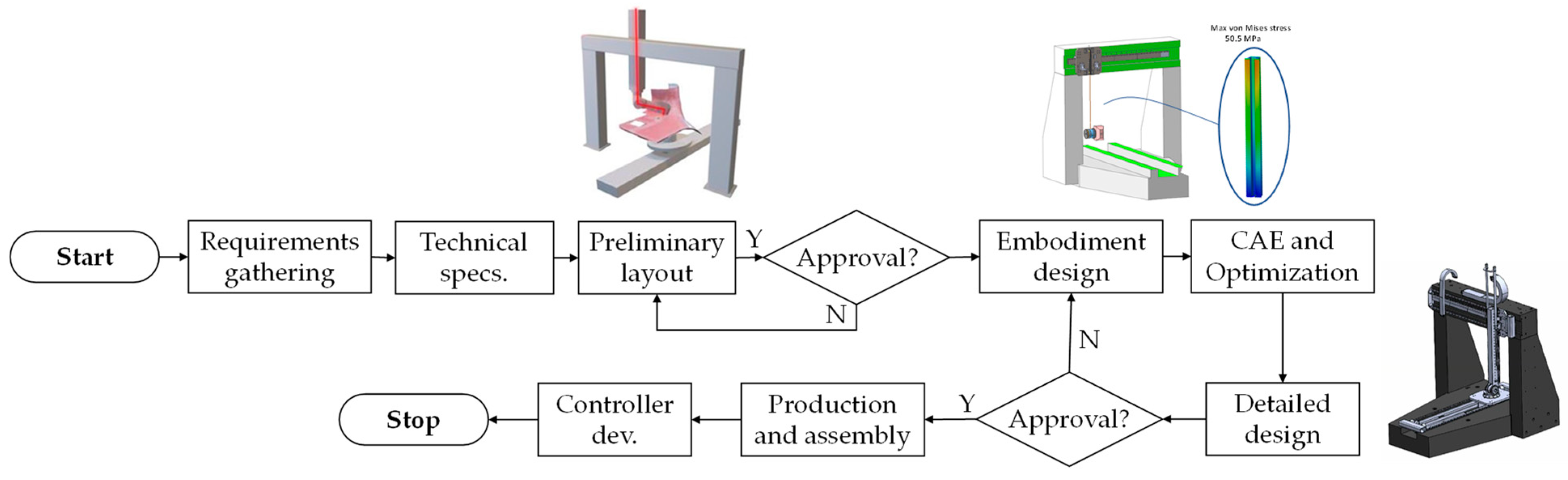
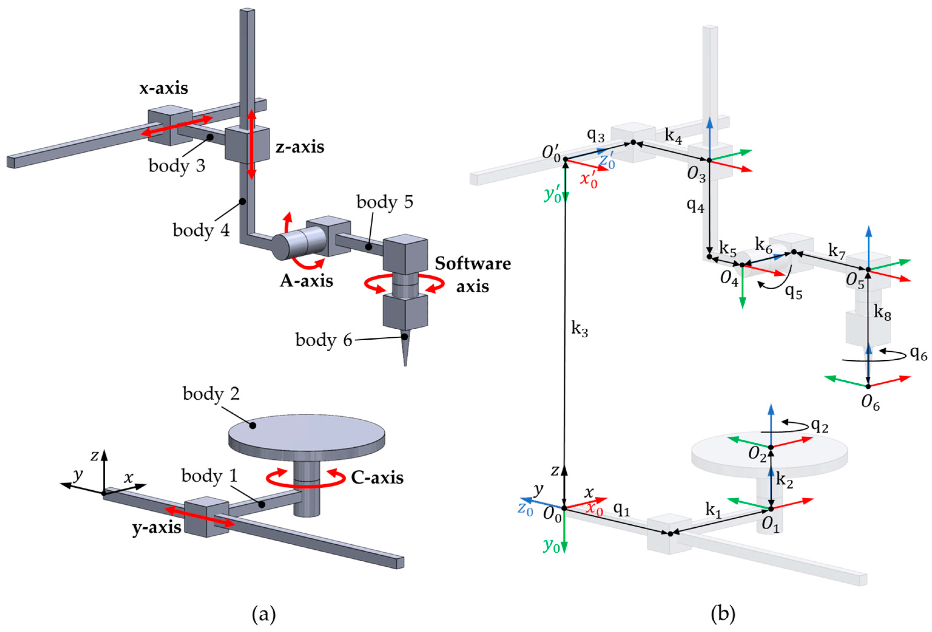
2. Overview of the OPeraTIC Manipulator

The design of the manipulator was driven by a deep analysis of project requirements, which were based on a comprehensive understanding of industrial needs and end-user expectations. These requirements were developed through detailed assessments across multiple sectors, ensuring that the machine would meet all functional requests. The study revealed a significant demand for surface texturing in various industries, aiming to gain competitive advantages through enhanced technical properties, improved energy efficiency, and the replacement of hazardous or environmentally harmful processes.

An example in the home appliance sector is shown in Figure 1a, where surface texturing enhances the hydrophobic properties of dishwasher baskets, reducing both water and energy consumption. In the automotive sector, as illustrated by the car closure in Figure 1b, technology reduces wear on stamping tools and improves lubrication, enabling the production of complex geometries and streamlining the manufacturing workflow. Another automotive application is in backlit surfaces within vehicle interiors, as shown in Figure 1c, where selective surface patterning optimizes light transmission and energy efficiency, supporting the development of customizable and energy-efficient solutions. In the aerospace industry, Figure 1d, surface treatment plays a crucial role in improving adhesion and paintability, eliminating the need for abrasive processes that are harmful to the environment, while also increasing repeatability.

These surface treatments can be successfully performed using laser microprocessing, a precise and efficient method for creating detailed textures and functional modifications on component surfaces [16]. However, this approach is typically limited to planar 2D operations, making it generally unsuitable for components with complex three-dimensional geometries [17,18]. The novel OPeraTIC manipulator is developed to address the need for working with components of widely varying shapes and sizes and to enable high-dynamics 3D processing with superior accuracy (in the order of microns).

The manipulator, depicted in Figure 2, features a granite base designed in a gantry configuration, with dimensions of 2300 × 2750 mm and a height of 2480 mm. The key advantage of this setup is a robust base that effectively dampens vibrations and ensures high structural rigidity that contributes to greater motion stability and accuracy under dynamic conditions [19,20]. The system offers five mechanical Degrees of Freedom (DoF), achieved through two decoupled kinematic chains comprising three linear axes (x, y, z) and two rotary axes (A, C) for orientation. The decision to split the kinematics into two chains was made to optimize the system dynamic behavior. This configuration was specifically chosen to avoid positioning two consecutive rotational axes, which would have unnecessarily complicated the machine’s kinematics. Additionally, such an arrangement would have increased inertia due to the extra motor mass and added complexity to the manipulator’s structure, making both assembly and mechanical integration more challenging. By considering also the additional rotational DoF provided by the laser scanner tool mounted at the end-effector, the chosen mechanical configuration allows for the full positioning and orientation of the workpiece in the Cartesian space, enabling complex machining operations on intricate 3D surfaces [21]. A rotary motor mounted on the y-axis carriage defines the C-axis, driving a rotating plate on which the workpiece will be fixed during processing. The second rotary motor, attached to the z-axis carriage, introduces the A-axis, allowing the mounted tool to rotate. To compensate gravitational forces on the vertically translating z-axis, two pneumatic cylinders are also employed. This design significantly reduces the load on the linear motor, which would otherwise need to bear the combined weight of the magnets and the tool.

As mentioned above, the manipulator is equipped with a galvanometric scanner, which generates a matrix of points during each scan to achieve the desired surface texturing.

This scanner allows for the shaping and orientation of the projected matrix on the workpiece’s surface, introducing an additional DoF that is not associated with a mechanical joint. Consequently, it is classified as a “software DoF” or “software axis”, as shown in Figure 3. While the galvanometric scanner is still under development and its geometry and mass properties remain undefined, a representative laser head has been used in this preliminary analysis to account for its inertia and volume properties.

The manipulator provides a cylindrical workspace with a diameter of 1600 mm and a height of 800 mm in order to satisfy the requirements to process large components. An efficient actuation system utilizing direct-drive motors has been selected, effectively minimizing positioning errors typically associated with traditional transmission systems, such as backlash and mechanical clearances [22,23,24,25].

Table 1. Characteristics of the installed commercial components on the manipulator axes.

Axis	Component	Description	Max Speed	Rated/Max Torque/Force
x	Servomotor	Tecnotion: UXX12	2.7 m/s	564/2800 N
	Encoder	Heidenhain: LIC 4113 (±3 µm)	10 m/s	-
	Guide	Bosch: 4 × R1651 7	5 m/s	-
y	Servomotor	Tecnotion: UXX18	2.7 m/s	846/4200 N
	Encoder	Heidenhain: LIC 4113 (±3 µm)	10 m/s	-
	Guide	Bosch: 4 × R1651 7	5 m/s	-
z	Servomotor	Tecnotion: UXX12	2.7 m/s	564/2800 N
	Encoder	Heidenhain: LIC 4113 (±3 µm)	10 m/s	-
	Guide	Bosch: 4 × R1651 2	5 m/s	-
	Pneumatic cylinder	SMC: 2 × RHCB50	3 m/s	1960 N
A	Servomotor	Tecnotion: QTR—A 133-60	724 rpm	21.9/35.3 Nm
	Encoder	Heidenhain ECA 4412 (±1.5″)	700 rpm	-
	Bearing	NSK: 2 × Super Precision 7013C	21,300 rpm	-
		NSK: 1 × 6908	13,000 rpm	-
C	Servomotor	Tecnotion: QTL—A 230-105	321 rpm	147/281 Nm
	Encoder	Heidenhain ECA 4412 (±1.5″)	5750 rpm	-
	Fifth wheel	Schaeffler: YRTC120-XL	900 rpm	-

offers a detailed description and highlights the key specifications of the components for each motion axis.

The process leading to the final manipulator design, outlined in Figure 4, is inherently iterative and highly dependent on precise evaluations to ensure optimal performance and reliability. Starting from the above-discussed technical specifications, a preliminary design was defined in CAD environment (SolidWorks 2024), which then underwent detailed engineering development and review. This phase typically relies on advanced CAE simulation tools to conduct comprehensive assessments. The simulation output guides decisions regarding the optimal dimensions of the manipulator links and the appropriate sizing of bearings, motors, and other mechanical components. However, this phase can be both resource-intensive and time-consuming, particularly when exploring large design domains (i.e., many variables) and addressing complex requirements. To overcome these challenges, one could also leverage analytical models, which can rapidly compute motions, joint forces, and torques; evaluate actuator requirements; and identify critical conditions such as singularities or unreachable points for several candidates, optimizing both the design and validation processes [26,27,28]. The adoption of accurate analytical models offers significant advantages during the control development phase as well [29,30]. Once the design phase is complete, these models will be integrated into the open controller module to enhance the system precision, responsiveness, and overall operational efficiency, aligning with the stringent requirements of modern manufacturing applications [31].

Based on these considerations, the following sections present the development of a detailed analytical behavioral model that comprehensively addresses the kinematics and dynamics of the OPeraTIC manipulator.

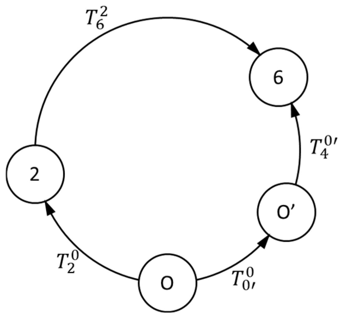
3. Kinematic Modeling

The functional schematic of the OPeraTIC manipulator, extracted from the CAD model reported in Figure 2, is presented in Figure 5a, detailing the components and identifying the revolute and prismatic joints responsible for their rotational and translational DoF. The first kinematic chain starts at the granite base and extends to the rotating table (body 2). It includes prismatic joint y-axis and revolute C-axis, providing two degrees of freedom (DoF). The second kinematic chain also starts at the base and reaches the laser (body 6), adding four more DoF. Along this chain, prismatic joints x-axis and z-axis are followed by revolute A-axis and software-axis, enabling precise control over the laser’s position and orientation. Each axis is represented as a joint, numbered consecutively starting from the base and continuing through to the final body in both kinematic chains.

Figure 5b provides a detailed representation of the reference frames that govern the system motion, structured according to the Denavit–Hartenberg (DH) convention. This formalism is utilized to accurately define the forward kinematics, which describe the relationship between the joint motions and the end-effector movements. The two kinematic chains are anchored at reference systems O and O’, respectively. Each joint is characterized by a base reference frame, $i-1$, and an active reference frame, $i$, which undergo relative motion through translation or rotation along the z-axis of the base reference frame. The displacement, whether angular or translational, of the joint corresponds to the variation of its associated DoF, denoted as $q_i$. The reference system $O_6$ is considered as the Tool Center Point (TCP), which corresponds to the projection of the laser that will then be directed onto the workpiece.

The parameters $k_j$, with $j=1,\dots ,8$, represent the DH parameters, which are fundamental in defining the kinematic model. The values are listed in

Table 2. Kinematic parameters of the OPeraTIC manipulator (values expressed in mm).

${\mathit{k}}_{\mathbf{1}}$	${\mathit{k}}_{\mathbf{2}}$	${\mathit{k}}_{\mathbf{3}}$	${\mathit{k}}_{\mathbf{4}}$	${\mathit{k}}_{\mathbf{5}}$	${\mathit{k}}_{\mathbf{6}}$	${\mathit{k}}_{\mathbf{7}}$	${\mathit{k}}_{\mathbf{8}}$
0	550.5	2170	75	160	200	400	250

, where the $k_6$, $k_7$ and $k_8$ were estimated by evaluating commercially available laser heads. According to the DH convention used in this representation, parameters $k_8$, $q_1$, and $q_4$ have negative values.

Once the reference frames are defined for each link, the DH parameters for both kinematic chains are easily assigned. These are listed in

Table 3. DH parameters of the first kinematic chain.

$\mathit{A}\mathit{x}\mathit{i}\mathit{s}$	$\mathit{d}$	$\mathit{\theta }$	$\mathit{a}$	$\mathit{\alpha }$
$1$ (y-axis)	$q_1$	$0$	$k_1$	$\pi /2$
$2$ (C-axis)	$k_2$	$q_2$	$0$	$0$

and

Table 4. DH parameters of the second kinematic chain.

$\mathit{A}\mathit{x}\mathit{i}\mathit{s}$	$\mathit{d}$	$\mathit{\theta }$	$\mathit{a}$	$\mathit{\alpha }$
$3$ (x-axis)	$q_3$	$0$	$k_4$	$\pi /2$
$4$ (z-axis)	$q_4$	$0$	$k_5$	$-\pi /2$
$5$ (A-axis)	$k_6$	$q_5$	$k_7$	$\pi /2$
$6$ (Software axis)	$k_8$	$\pi /2+q_6$	$0$	$0$

. Each row of the table allows for the definition of the relative transformation matrix ${\mathit{T}}_{\mathit{i}}^{\mathit{i}\mathbf{-}\mathbf{1}}$ between reference frame $i$ and frame $i-1$. By post-multiplying the six transformation matrices, the overall transformation matrix for both the kinematic chains can be obtained as follow:

$${\mathit{T}}_{\mathbf{2}}^{\mathbf{0}}\left(q_i\right)={\mathit{T}}_{\mathbf{1}}^{\mathbf{0}}{\mathit{T}}_{\mathbf{2}}^{\mathbf{1}}$$

(1)

$${\mathit{T}}_{\mathbf{6}}^{\mathbf{0}}\mathbf{\prime }\left(q_i\right)={\mathit{T}}_{\mathbf{3}}^{\mathbf{0}}\mathbf{\prime }\mathbf{\dots }{\mathit{T}}_{\mathbf{6}}^{\mathbf{3}}$$

(2)

During the trajectory definition process, it is often beneficial to describe the motion of the TCP within a reference frame fixed to the workpiece. To achieve this, it is necessary to establish the transformation between the rotating table, which is securely attached to the workpiece, and the TCP. By understanding the transformations from the base frame to the rotating table and from the base frame to the TCP, we can derive the desired transformation. However, an additional transformation is needed to account for the static relationship between the original reference frame, O, and the newly defined reference frame, O′. The flow of transformations is illustrated in Figure 6.

Therefore, the transformation of interest can be derived as:

$${\mathit{T}}_{\mathbf{6}}^{\mathbf{2}}\mathbf{=}{{{\mathit{T}}_{\mathbf{2}}^{\mathbf{0}}}^{\mathbf{-}\mathbf{1}}\mathit{T}}_{{\mathbf{0}}_{\mathbf{\prime }}}^{\mathbf{0}}{\mathit{T}}_{\mathbf{6}}^{{\mathbf{0}}_{\mathbf{\prime }}}$$

(3)

where:

$${\mathit{T}}_{{\mathit{O}}_{\mathbf{\prime }}}^{\mathit{O}}=\left[\begin{array}{cccc}0& 0& 1& 0\\ 0& 1& 0& {-k}_3\\ -1& 0& 0& 0\\ 0& 0& 0& 1\end{array}\right]$$

(4)

This transformation represents the rotation and translation of reference frame O′ with respect to reference frame O. The result enables the computation of the TCP pose given the joint values. The pose is typically expressed using Cartesian coordinates (x, y, z) and orientations defined by the roll (R), pitch (P), and yaw (Y) angles. However, since these equations will be used in a real control system, it is more advantageous to represent the rotations using unit quaternions rather than a rotation matrix. The quaternion representation has several advantages:

• Compactness: quaternions require only four parameters compared to the nine elements of a rotation matrix, reducing the computational overhead.
• Avoidance of Gimbal Lock: unlike Euler angles, quaternions do not suffer from gimbal lock, allowing for smooth interpolations and rotations.
• Efficient Computation: rotations represented by quaternions are more computationally efficient, especially when combining multiple rotations.

From this process, it is possible to obtain a seven-component vector, which is divided into a Cartesian position vector and a quaternion ($q_x,q_y, q_z, q_w)$ that defines the pose of reference frame 6 relative to frame 2.

$$\mathit{p}=\left[\begin{array}{c}\begin{array}{c}x\\ y\\ z\end{array}\\ \begin{array}{c}{q}_x\\ q_y\\ q_z\end{array}\\ q_w\end{array}\right]=\left[\begin{array}{c}\begin{array}{c}({-k}_1+k_6+q_3)cos\left(q_2\right)+({-k}_4-k_5-k_{7}cos\left(q_5\right)-k_{8}sin\left(q_5\right)-q_1)sin\left(q_2\right)\\ (k_1-k_6-q_3)sin\left(q_2\right)+(-k_4-k_5-k_{7}cos\left(q_5\right)-k_{8}sin\left(q_5\right)-q_1)cos\left(q_2\right)\\ -k_2+k_3-k_{7}sin\left(q_5\right)+k_{8}cos\left(q_5\right)+q_4\end{array}\\ \begin{array}{c}sin(q_5/2)cos(q_2/2+q_6/2)\\ -sin(q_5/2)sin(q_2/2+q_6/2)\\ -cos(q_5/2)sin(q_2/2-q_6/2)\end{array}\\ cos(q_5/2)cos(q_2/2-q_6/2)\end{array}\right]$$

(5)

By utilizing the direct kinematics equations, it is possible to analytically derive the inverse kinematics equations. The inverse kinematics analysis aims to determine the joint positions given the TCP desired position. The joint equations can be derived by analyzing the above equation, considering the pose vector as the input.

By taking the first three components of the pose vector $\mathit{p}$ and considering x, y, and z as inputs, it is possible to solve the system of equations by assuming $q_1$, $q_3$, and $q_4$ as unknowns variables.

$$q_1={-k}_4{-k}_5{-k}_{7}cos\left(q_5\right)-k_{8}sin\left(q_5\right)-xsin\left(q_2\right)-ycos\left(q_2\right)$$

(6)

$$q_3=k_1{-k}_6+xcos\left(q_2\right)-ysin\left(q_2\right)$$

(7)

$$q_4=k_2{-k}_3+k_{7}sin\left(q_5\right)-k_{8}cos\left(q_5\right)+\mathrm{z}$$

(8)

$q_1$ and $q_3$ still depend on $q_2$ e $q_5$, which remain unknowns. By applying the same procedure to the fourth, fifth, and sixth components of the pose vector $\mathit{p}$ and solving in terms of $q_2$ and $q_5$ and $q_6$, it is possible to express $q_5$ independently of the other joints:

$$q_5=\pm 2asin\left(\sqrt{{q_x}^2+{q_y}^2}\right)$$

(9)

As can be seen from Equation (5), there is a sign indeterminacy, indicating that there are two possible configurations of the manipulator. With further elaboration, one could obtain:

$$\mathrm{s}\mathrm{i}\mathrm{n}{\displaystyle \frac{q_5}{2}}=\pm \sqrt{{q_x}^2+{q_y}^2}$$

(10)

which can also be rewritten as:

$${\sin }^2\left({\displaystyle \frac{q_5}{2}}\right)={q_x}^2+{q_y}^2=1-{q_z}^2-{q_w}^2$$

(11)

The equality expressed in Equation (11) is valid since the sum of the squares of the components of a unit quaternion equals 1. Consequently:

$$\mathit{cos}\left({\displaystyle \frac{q_5}{2}}\right)=\sqrt{{q_z}^2+{q_w}^2}$$

(12)

Through straightforward trigonometric steps, starting from the last four components of Equation (5), it can be deduced that:

$${\displaystyle \frac{q_2}{2}}+{\displaystyle \frac{q_6}{2}}=\mathrm{atan}2\left(-{\displaystyle \frac{q_y}{\sin \left(\frac{q_5}{2}\right)}},{\displaystyle \frac{q_x}{\sin \left(\frac{q_5}{2}\right)}}\right)$$

(13)

$${\displaystyle \frac{q_2}{2}}-{\displaystyle \frac{q_6}{2}}=\mathrm{atan}2\left(-{\displaystyle \frac{q_z}{\cos \left(\frac{q_5}{2}\right)}},{\displaystyle \frac{q_w}{\cos \left(\frac{q_5}{2}\right)}}\right)$$

(14)

The final expression of $q_2$ and $q_6$ can thus be identified as:

$$q_2=\mathrm{atan}2\left(-{\displaystyle \frac{q_y}{\pm \sqrt{{q_x}^2+{q_y}^2}}},{\displaystyle \frac{q_x}{\pm \sqrt{{q_x}^2+{q_y}^2}}}\right)+\mathrm{atan}2\left(-{\displaystyle \frac{q_z}{\sqrt{{q_z}^2+{q_w}^2}}},{\displaystyle \frac{q_w}{\sqrt{{q_z}^2+{q_w}^2}}}\right)$$

(15)

$$q_5=2acos(\pm \sqrt{{q_x}^2+{q_y}^2})$$

(16)

$$q_6=\mathrm{atan}2\left(-{\displaystyle \frac{q_y}{\pm \sqrt{{q_x}^2+{q_y}^2}}},{\displaystyle \frac{q_x}{\pm \sqrt{{q_x}^2+{q_y}^2}}}\right)-\mathrm{atan}2\left(-{\displaystyle \frac{q_z}{\sqrt{{q_z}^2+{q_w}^2}}},{\displaystyle \frac{q_w}{\sqrt{{q_z}^2+{q_w}^2}}}\right)$$

(17)

The inverse kinematics yields two possible solutions, corresponding to two distinct configurations of the manipulator shown in Figure 7. These configurations arise from the ability to approach the rotating table with either $q_5>0$ or $q_5<0$ by adding a rotation of $\pi /2$ to the rotating table. To calculate the velocities and accelerations of the TCP as a function of the joints, or vice versa, it is necessary to conduct a differential kinematic analysis and thus determine the 6 × 6 Jacobian matrix J of the system.

$$\mathit{J}=\left[\begin{array}{cc}\begin{array}{ccc}{\displaystyle \frac{\mathsf{\partial }x}{\mathsf{\partial }{q}_1}}& {\displaystyle \frac{\mathsf{\partial }x}{\mathsf{\partial }{q}_2}}& \cdots \end{array}& {\displaystyle \frac{\mathsf{\partial }x}{\mathsf{\partial }{q}_n}}\\ \begin{array}{ccc}{\displaystyle \frac{\mathsf{\partial }y}{\mathsf{\partial }{q}_1}}& {\displaystyle \frac{\mathsf{\partial }y}{\mathsf{\partial }{q}_2}}& \cdots \end{array}& {\displaystyle \frac{\mathsf{\partial }y}{\mathsf{\partial }{q}_n}}\\ \begin{array}{ccc}{\displaystyle \frac{\mathsf{\partial }z}{\mathsf{\partial }{q}_1}}& {\displaystyle \frac{\mathsf{\partial }z}{\mathsf{\partial }{q}_2}}& \cdots \end{array}& {\displaystyle \frac{\mathsf{\partial }z}{\mathsf{\partial }{q}_n}}\end{array}\right]$$

(18)

The first three rows of the matrix are simply derived by differentiating the previously defined direct kinematics equations. To derive the second part of the Jacobian, which is related to the angular velocity, it is necessary to determine the axes of the angular velocities for each joint in the reference frame of the rotating table. Indeed, the angular velocity of each joint is given by the product of the unit vector of the angular velocity and its magnitude, which corresponds to the derivative of the DoF itself.

$${\mathit{\omega }}_{\mathit{i}}={\widehat{\mathit{\omega }}}_{\mathit{i}}{\dot{q}}_i=\left[\begin{array}{c}{a}_1\\ a_2\\ a_3\end{array}\right]{\dot{q}}_i$$

(19)

The procedure is straightforward since the relative transformations between the various reference frames are already known from inverse kinematics. Moreover, it shall be noted that only the revolute joints 1, 5, and 6 contribute to defining the angular velocity of the TCP. As a first step, it is necessary to define the unit vectors of the angular velocities for each joint in the reference frame of the rotating table. By utilizing the transformations from direct kinematics and the DH convention, and focusing on the joint of interest $i$, it is possible to derive these unit vectors as they correspond to the third column of the transformation matrix:

$${\mathit{T}}_{\mathit{i}}^{\mathbf{2}}=\left[\begin{array}{cccc}\cdots & \cdots & a_1& \cdots \\ \cdots & \cdots & a_2& \cdots \\ \cdots & \cdots & a_3& \cdots \\ 0& 0& 0& 1\end{array}\right]\to {\widehat{\mathit{\omega }}}_{\mathbf{i}}^{\mathbf{2}}=\left[\begin{array}{c}{a}_1\\ a_2\\ a_3\end{array}\right]$$

(20)

The complete Jacobian matrix is then expressed as follows:

$$\mathit{J}=\left[\begin{array}{cc}\begin{array}{cc}{\displaystyle \frac{\mathsf{\partial }x}{\mathsf{\partial }{q}_1}}& {\displaystyle \frac{\mathsf{\partial }x}{\mathsf{\partial }{q}_2}}\\ {\displaystyle \frac{\mathsf{\partial }y}{\mathsf{\partial }{q}_1}}& {\displaystyle \frac{\mathsf{\partial }y}{\mathsf{\partial }{q}_2}}\end{array}& \begin{array}{cc}\begin{array}{cc}{\displaystyle \frac{\mathsf{\partial }x}{\mathsf{\partial }{q}_3}}& \cdots \end{array}& {\displaystyle \frac{\mathsf{\partial }x}{\mathsf{\partial }{q}_1}}\\ \begin{array}{cc}{\displaystyle \frac{\mathsf{\partial }y}{\mathsf{\partial }{q}_3}}& \cdots \end{array}& {\displaystyle \frac{\mathsf{\partial }y}{\mathsf{\partial }{q}_n}}\end{array}\\ \begin{array}{cc}{\displaystyle \frac{\mathsf{\partial }z}{\mathsf{\partial }{q}_1}}& {\displaystyle \frac{\mathsf{\partial }z}{\mathsf{\partial }{q}_2}}\\ {\widehat{\mathit{\omega }}}_{\mathbf{2}}^{\mathbf{2}}& {\widehat{\mathit{\omega }}}_{\mathbf{1}}^{\mathbf{2}}\end{array}& \begin{array}{cc}\begin{array}{cc}{\displaystyle \frac{\mathsf{\partial }z}{\mathsf{\partial }{q}_3}}& \cdots \end{array}& {\displaystyle \frac{\mathsf{\partial }z}{\mathsf{\partial }{q}_n}}\\ \begin{array}{cc}{\widehat{\mathit{\omega }}}_{\mathbf{3}}^{\mathbf{2}}& \cdots \end{array}& {\widehat{\mathit{\omega }}}_{\mathit{n}}^{\mathbf{2}}\end{array}\end{array}\right]$$

(21)

The elements of the $\mathit{J}$ matrix are detailed in the Appendix A. From this matrix, joint velocities and accelerations can be calculated given the Cartesian velocity and acceleration. Additionally, by calculating the determinant of the Jacobian matrix, the singular configurations of the manipulator can be determined as:

$$det\left(\mathit{J}\right)=0\to sin\left(q_5\right)=0\to q_5=0,\pi$$

(22)

The manipulator is thus in a singular configuration when the axis of joint 6 is perpendicular to the rotating table.

4. Dynamic Modeling

The dynamic analysis aims to calculate the joint forces/torques required to achieve the desired motion of the machine. This analysis was conducted using the Newton–Euler formulation as outlined in [32]. To streamline the analysis while preserving accuracy, several assumptions were made:

• All components are modeled as rigid bodies.
• The force in the pneumatic cylinders is assumed to be constant (i.e., no fluctuations).
• External process forces acting on the system are neglected.
• Viscous friction is ignored, and only Coulomb friction is considered.

The rigid body assumption holds, as the manipulator’s components are designed to be highly stiff, ensuring that deformation under load is negligible and does not impact the analysis. The simplification of constant force in the pneumatic cylinders is noteworthy, as in reality such forces depend on factors like axis speed, acceleration, and air temperature. These variables are here omitted to focus on the primary dynamic contributions of the system. Additionally, since no external forces act on the rotating platform or the laser head (differently from CNC machines), these forces are set to zero in the model. Lastly, the mass of body 6 is assumed to be zero, as it represents the laser beam itself rather than a physical component of the manipulator. By making these assumptions, the dynamic model achieves a balance between simplicity and accuracy, capturing the key aspects of the system’s behavior while enabling efficient force/torque calculations to support design and control development.

The resulting dynamic equation is as follows [32]:

$$\mathit{Q}=\mathit{B}\left(\mathit{q}\right)\ddot{\mathit{q}}+\mathit{C}\left(\mathit{q},\dot{\mathit{q}}\right)\dot{\mathit{q}}+{\mathit{F}}_{\mathit{s}}sgn\left(\dot{\mathit{q}}\right)+\mathit{g}\left(\mathit{q}\right)$$

(23)

In the equation $\mathit{q}$, $\dot{\mathit{q}}$, and $\ddot{\mathit{q}}$ stand for the vector of joints position, velocity, and acceleration, respectively. These quantities can be computed using the methods detailed in the previous chapter. Additionally, $\mathit{Q}$ is the vector of generalized forces (forces or torques exerted by the joints), $\mathit{B}\left(\mathit{q}\right)$ is the mass (or inertia) matrix, $\mathit{C}\left(\mathit{q},\dot{\mathit{q}}\right)$ is the Coriolis matrix, ${\mathit{F}}_{\mathit{s}}$ is the diagonal matrix of Coulomb friction forces for each axis, $\mathit{g}\left(\mathit{q}\right)$ is the vector of gravitational forces. The resolution of the dynamics thus reduces to determining these components for both kinematics chains. The matrix ${\mathit{F}}_{\mathit{s}}$, given the assumptions made, can be readily determined. The elements corresponding to the translational joints are calculated by multiplying the normal force acting on the joint by the static friction coefficient. For the rotational joints, an additional multiplication by the radius of the inner bearing ring is required to compute the static friction torque.

The dynamic analysis is performed in two main steps. First, the velocities and accelerations of each link are calculated, starting from the base and moving to the end-effector. In this step, the kinematic models and DH transformations, discussed in Section 3, are utilized. Next, the forces and torques on each joint are computed by starting at the end-effector and moving backward through the links. This phase requires defining the inertia matrices $\mathit{I}$ in the center mass reference system, masses $m_i$, and center of mass positions ${\mathit{r}}_{\mathit{i}}=({x_{cm}}_i,{y_{cm}}_i,{z_{cm}}_i)$ for each link $i$. These quantities, derived from the CAD model, are constant as they are defined within the reference frame rigidly attached to the body. Since external forces on individual links are ignored in this analysis, the effect of the pneumatic pistons is not considered at first sight. However, an additional force term has to be added to the dynamic equation of z-axis driving force, equal to:

$$F_p=-(m_4+m_5)g$$

(24)

where $m_4$ and $m_5$ represent the masses to be supported by the pistons, whereas $g$ is the gravitational acceleration. By solving the recursive procedure, it is therefore possible to derive $\mathit{B}\left(\mathit{q}\right)$, $\mathit{C}\left(\mathit{q},\dot{\mathit{q}}\right)$, and $\mathit{g}\left(\mathit{q}\right)$ for both kinematic chains. These results are provided in Appendix A. By analyzing these components, it is evident that the positions of the center of mass and the inertia of the translational bodies do not influence the definition of the driving forces. This occurs because in the current architecture there are no prismatic joints preceded by a rotational joint. Additionally, it can be observed that for the bodies 2 and 5, only the moments of inertia ${I_{zz}}_2$ and ${I_{yy}}_5$, respectively, are involved. This is due to the absence of two or more consecutive rotational joints within a single kinematic chain. As a result, the rotation axis of these bodies remains fixed over time. The inertial parameters associated with the manipulator, which are essential for solving the corresponding equations, are presented in

Table 5. Dynamic parameters of the bodies (links): mass, center of mass position and inertia values.

Link	$\mathit{m}$ [kg]	${\mathit{x}}_{\mathit{c}\mathit{m}}$ [mm]	${\mathit{y}}_{\mathit{c}\mathit{m}}$ [mm]	${\mathit{z}}_{\mathit{c}\mathit{m}}$ [mm]	$\mathit{I}$ [kgmm2]
1	158.8	-	-	-	-
2	26.2	0	0	0	164,287.2
3	131.6	-	-	-	-
4	125.0	-	-	-	-
5	5.8	0	0	−325	6796.4

. As said, these properties were estimated from the CAD model within SolidWorks. For the first kinematic chain, the flange serves as the final coupling device with the workpiece, for the second, it instead couples with the laser head.

Regarding the calculation of frictional forces, all the coefficients have been carefully extracted from the manufacturer catalogs. In particular, for the linear guides with ball recirculation, a Coulomb static friction coefficient of 0.003 is considered, which will be multiplied by the normal force acting on the joint. For C-axis, a constant friction torque of 4 Nm is provided. Finally, for the rotating A-axis, the friction coefficient given by the bearings is 0.0040.

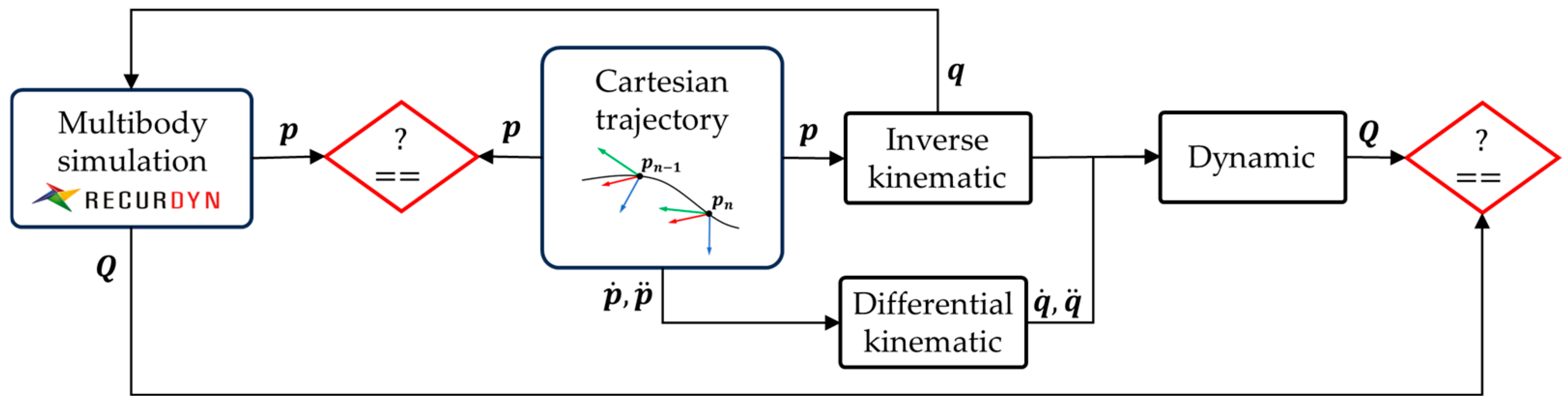
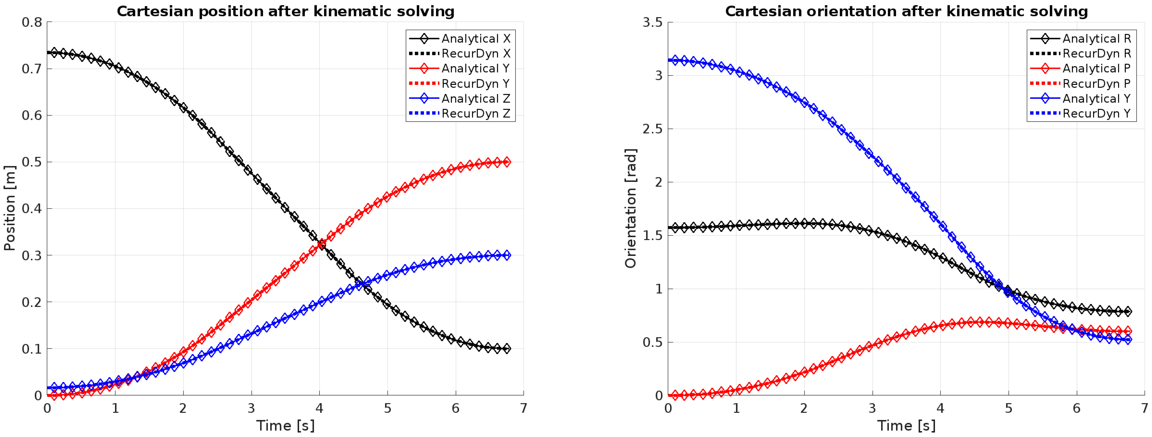
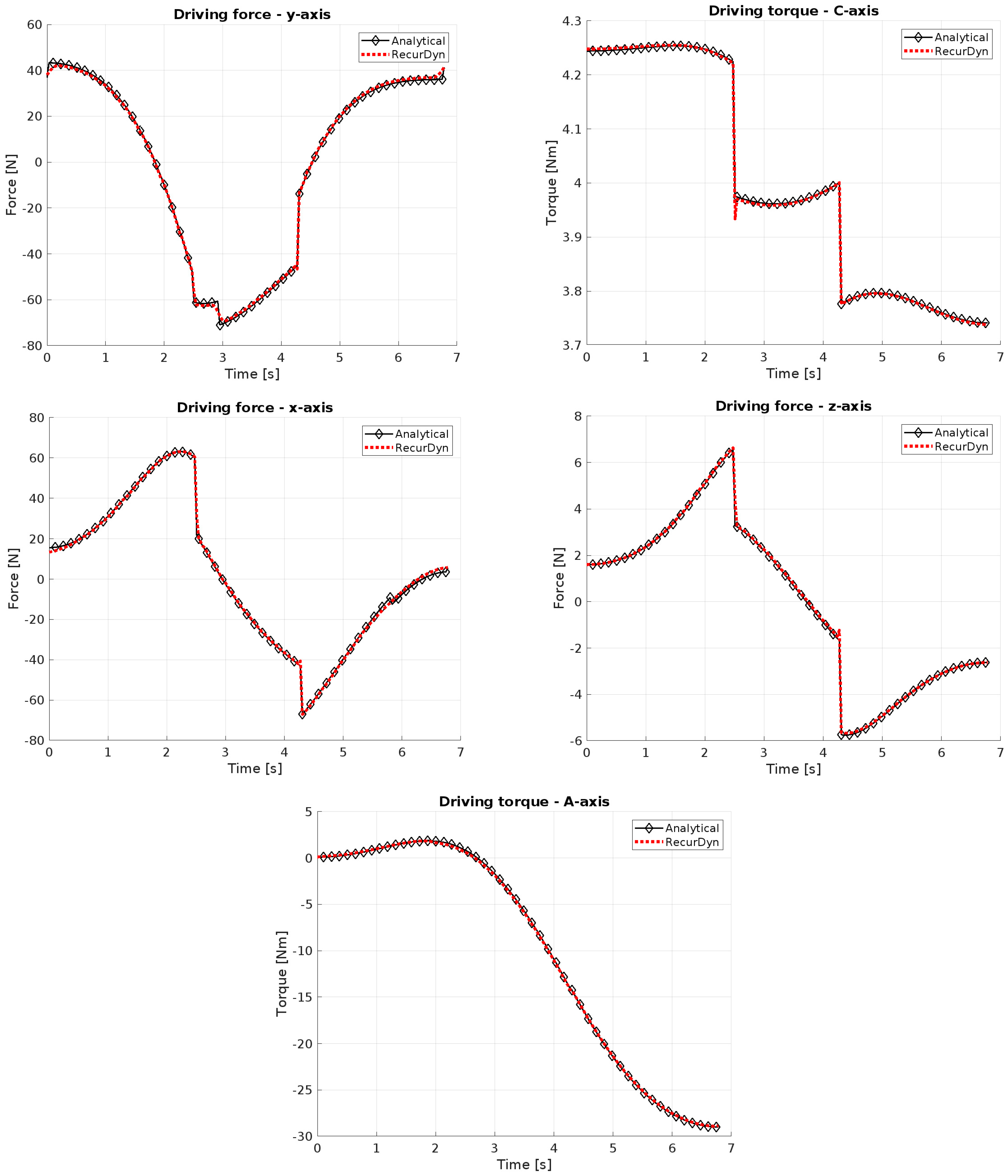
5. Model Validation and Performance Maps

The theoretical models presented in Section 3 and Section 4 have been coded and solved within Python (3.13.0). To verify their correctness, a CAE model of the manipulator was developed and simulated in RecurDyn (V2024). To ensure consistency between the models, the virtual prototype in RecurDyn assumes rigid links, idealized joints without clearance, and massless joints. The tests were conducted under specific parameters.

5.1. Test on Linear Path

Initially, a linear path, typically executed in this type of machine through a G01 G-code command, was imposed using a trapezoidal velocity timing law. The motion of interest is described in the reference frame of the rotating table, as detailed in Section 3. It consists of a Cartesian translation (x, y, z) and rotations around the roll, pitch, and yaw angles (R, P, Y), with translation and rotation occurring synchronously. This motion was specifically chosen to be non-aligned with any machine axis, enabling the involvement of all axes in the inverse kinematics solution and ensuring the complete validation of the analytical models. In this test, a null payload (no workpiece) was considered on the rotating plate (first kinematic chain), while the laser head was mounted on the A-axis (second kinematic chain). The maximum imposed linear velocity and acceleration are respectively 150 mm/s and 60 mm/s². The generated trajectory was discretized into 200 points. For each trajectory point, the numerical models solved the inverse kinematics and dynamics to calculate the joint positions, velocities, accelerations, and the driving forces/torques. Based on the chart depicted in Figure 8, the computed joint positions were utilized in RecurDyn to simulate the resulting TCP trajectory, joint velocities, and torques. The outcomes of the CAE simulation were then compared with the theoretical results to assess the model validity [33,34].

The plots in Figure 9 clearly demonstrate that the positions and orientations predicted by the theoretical model are fully aligned with the ones achieved in RecurDyn. However, slight differences (in the order of 1.8%) emerge in the driving forces and torques plots shown in Figure 10. These variations can be attributed to the use of more detailed and realistic friction models within RecurDyn, in contrast to the simplified assumptions employed by the analytical model. Additionally, the analysis of joint 5 reveals that the required torque, considering the specified motion along with the mass and center of mass position of the laser head, significantly exceeds the nominal torque deliverable by the motor and approaches its peak torque limit. This underlines the importance of evaluating manipulator performance early in the design phase to avoid situations where design requirements are not met.

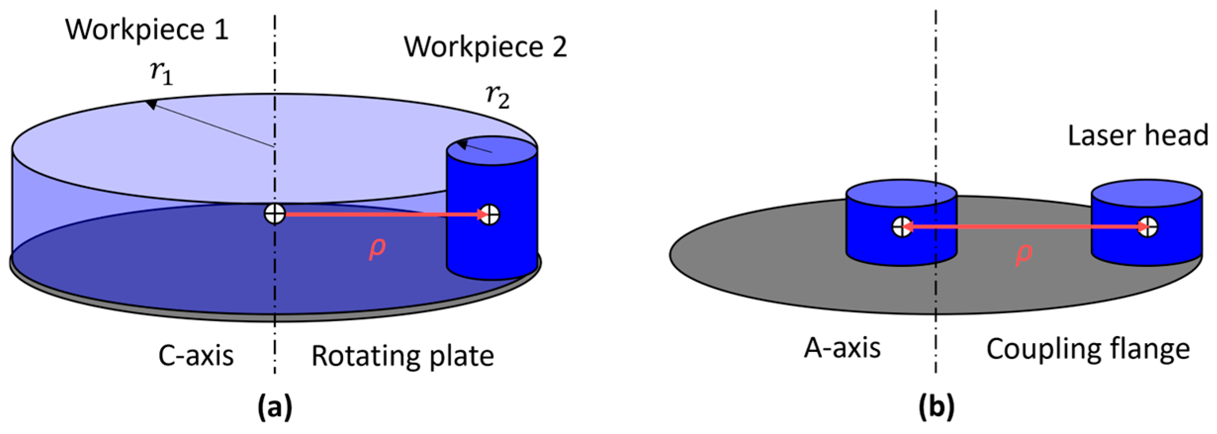
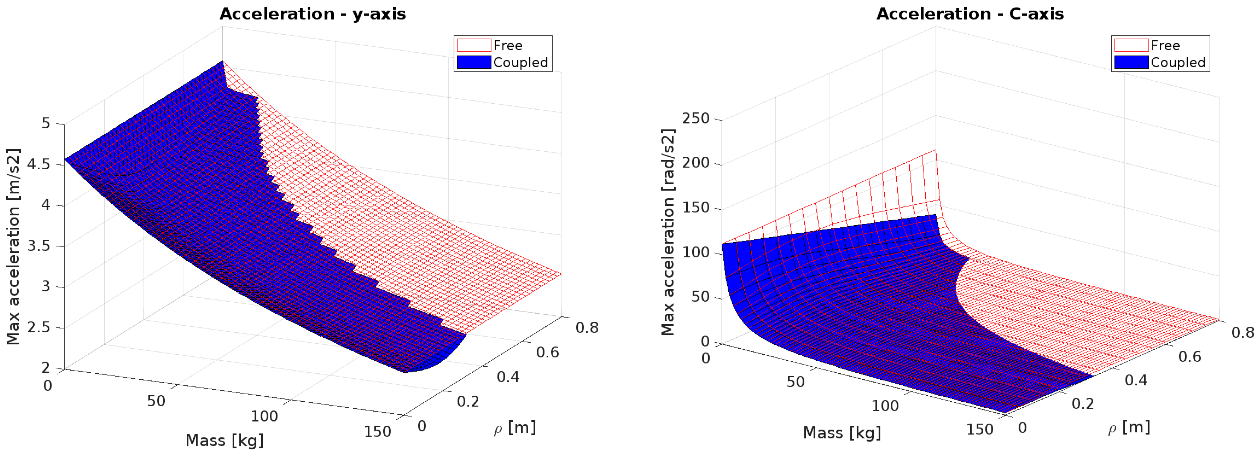
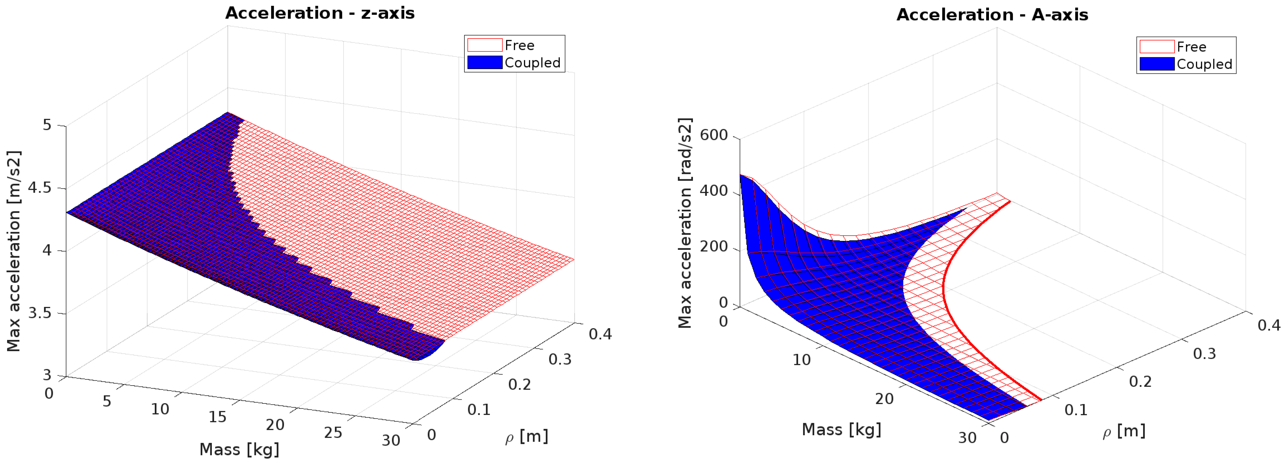
5.2. Effect of Payload Distribution

The performance of the manipulator is strongly influenced by the mass properties of the workpiece and the laser head. This is because these are mounted at the ends of the two kinematic chains (the workpiece on the rotary table and the laser head on the flange). The addition of mass or inertia can result in the machine motors being unable to perform the required motion due to exceeding torque limits. Conversely, it is also necessary to analyze the performance when the components have reduced mass or inertia, as highly dynamic motion could demand speeds or accelerations that exceed the limits of one or more joints.

For this reason, the study of the manipulator performance considers the mass properties of the workpiece and the laser head as variable parameters to define the operating range and limits of the machine. The following assumptions have been made to simplify the analysis:

Workpiece Assumptions: the geometry and mass properties of the workpiece vary across use cases. In this preliminary study, the workpiece was approximated as a uniformly dense cylinder, with its radius adjusted according to workspace utilization. Specifically, the radius decreases as the object moves outward from C-axis, as illustrated in Figure 11a. By varying the radius, the mass and inertia of the body also change accordingly.

Laser Head Assumptions: the laser head presents fixed mass and inertia matrix values. Its positioning relative to A-axis can vary depending on the design phase. The head can be thus approximated as a cylinder positioned at a distance $\rho$ from the rotation axis (Figure 11b). Additionally, in the actual operation of the machine, the laser head will not be able to rotate freely around the A-axis but will be limited to tilting motions. Despite this, in the current validation joint limits are not considered to simulate worst-case usage scenarios.

By exploiting the proposed analytical models, a parametric study has been conducted to generate the performance map of each axis in terms of maximum achievable acceleration under different combinations of payload mass and center of mass eccentricity ($\rho$). For the axes of the first kinematic chain, the mass properties of the workpiece are considered, while for the axes of the second kinematic chain, these properties correspond to the laser head. The axis actuation can be analyzed in two scenarios:

Free: each axis moves independently while the others remain stationary.

Coupled: in this case the effect of mutual dynamic interactions between different axes is enabled. In practice, each axis is subject to forces and torques generated by other motors. In this analysis, the worst-case scenario, involving maximum external interference, is considered.

Motors are assumed to operate at nominal force/torque, which corresponds to the level that can deliver indefinitely (equivalent to a 100% duty cycle). The results of this study are reported and commented on hereinafter. The imposed motion involves a single acceleration ramp, without the need to define an entire trajectory.

The results for the first kinematic chain, specifically for the y-axis and C-axis, are shown in Figure 12. Notably, some portions of the 3D performance surface in the case of coupled are missing. These gaps represent scenarios in which the payload conditions exceed the manipulator capabilities. Specifically, they occur when the rotational C-axis is unable to generate sufficient torque to counteract the maximum acceleration demanded by the linear y-axis. In these cases, the required torque surpasses the motor capacity, making it impossible for the system to interpolate movements along the required trajectory. Such conditions are effectively unfeasible, as the manipulator cannot execute the motion within the given constraints.

The performance of the z-axis and A-axis are shown in Figure 13. Analyzing the plot for the A-axis, it can be observed that a static loading limit exists. This limit is represented by the red curve on the Mass-CM Distance plane (with the maximum acceleration equal to zero). The curve indicates the maximum weight the A-axis can handle under static conditions, as a function of the distance from the rotation axis, without causing motor overheating. In the coupled condition, where the z-axis also moves, the capacity of the A-axis to withstand a static load is further reduced. This implies that as the z-axis exerts additional force, the ability of the A-axis to support static loads becomes increasingly constrained. The performance of z-axis is instead enhanced by pneumatic piston support (considered in the dynamic model), which helps counteract the gravitational forces acting on the system. Without this pneumatic support, the motor driving the z-axis would be unable to maintain its position against gravity indefinitely. This is evident in Figure 13, where the maximum achievable acceleration is lower than the gravitational acceleration. The increased workload in scenarios without pneumatic assistance could lead to overheating, with the serious risk of motor damage or failure.

The x-axis represents a unique case, as its motion capabilities are not influenced by coupling with the other manipulator axes. In fact, by analyzing the resolved dynamics equation (Equation (23)), it can be observed that the axes connected to it do not affect the force required for its motion. Despite being decoupled from other axes movement, its acceleration is significantly limited by the high payload. As can be noted in Figure 14, with a maximum value of 2 m/s², its acceleration is considerably lower than that of the other linear axes.

The performance maps discussed so far have been obtained by considering the nominal operation of the motors. However, motors can exceed these values and operate at higher levels for short periods, until reaching the peak force/torque. This allows for a significant increase in the manipulator performance, but only for brief durations, as in this range the motors experience a rapid temperature increase, reaching up to 6 °C/s at peak values. For this reason, the machine performance was analyzed also considering the motors operating at their peak force/torque output. In this case, only the coupled operation scenario is considered, as it was observed in previous cases that the simultaneous motion of multiple axes creates the most critical conditions. In Figure 15, the volumes below the surfaces (motor peak area and motor continuous area) represent the permissible operating ranges for the axes, expressed dimensionally as 3D volumes. The plots highlight how linear axes have the greatest variation in performance due to their high difference between peak and nominal levels.

Another parameter to consider in order to complete the performance analysis is the maximum allowable speed for each axis. This is significantly influenced by the shape of the timing law used for trajectory generation. In this study, a trapezoidal profile is employed to demonstrate maximum speed performance. In particular, the maps are generated for every axis by considering different combinations of payloads and strokes. This profile enables rapid execution of movements, although a notable drawback is the lack of smooth transitions between acceleration, constant velocity, and deceleration phases, which can induce mechanical stress and vibrations in the system. To address these issues and enhance the machine performance and reliability, a Double-S timing law will be effectively implemented in the real controller. This adjustment aims to provide smoother transitions between acceleration and deceleration phases, thereby reducing mechanical stress and extending the system lifespan.

From Table 1, the maximum allowed speed is 2.7 m/s for all linear motors, 33.6 rad/s for the C-axis and 75.8 rad/s for the A-axis. However, as visible in Figure 16, the A-axis is the only one unable to reach its maximum speed under optimal conditions (minimum payload and maximum stroke). Instead, its speed is limited to just over 40 rad/s, falling short of the specified 75.8 rad/s. It is important to note that the speed of each axis ultimately depends on the trajectory being executed. Therefore, the performance presented in these graphs represents theoretical maximums. For a more realistic application scenario, refer to the analysis provided in the following section.

5.3. Test on Circular Path

The last test involves simulating the execution of a spatial movement, typically using a S-shaped curve (also named Scone curve) [35] or a circle [36,37]. However, as in the previous Sections, the computed driving forces/torques are not affected by any contribution coming from direct interaction among the tool and the workpiece (e.g., cutting forces), as normally happens in CNC machines [38,39,40]. The path chosen for the test is inspired by ISO 9283 norm, dedicated to IR accuracy assessment. Inside the ISO cube, the biggest circular path has been chosen for the translational part of the path. Concerning the rotational axes, custom orientation paths were generated using Spherical Linear interpolation (SLERP) between initial and final states, ensuring comprehensive evaluation of the manipulator capabilities. The resulting path defined is depicted in Figure 17.

In this case, a jerk-limited timing law has been chosen to simulate the real behavior of the manipulator and to avoid abrupt movements and vibrations in the motors. In order to proceed with the test, it is essential to fully define the inertial parameters of the moving components, including the workpiece and the laser head, as well as the parameters for velocity, acceleration, jerk, and circle radius to define the trajectory. These parameters, listed in

Table 6. Parameters selected to execute the reference path.

Parameter	Value	Parameter	Value
Circle radius [mm]	509.12	Workpiece [kg]	75
Velocity [mm/s]	2000	Laser head [kg]	20
Acceleration [mm/s2]	3200	Workpiece ρ [mm]	20
Jerk [mm/s3]	20000	Laser ρ [mm]	75

, were chosen based on the guidelines provided by industrial partners and represent a typical use case for the machine under design.

The obtained trajectory, discretized into 200 points, has a duration slightly over 2 s. As seen in Figure 18, rotational movements are very short in the path, and due to synchronization between translational and rotational motions, the speeds are significantly lower than the nominal speeds of the axes. Some motors temporarily operate beyond their continuous operation range but remain within the peak performance limits. This is acceptable for short durations, provided that the operating time is carefully monitored to avoid overheating or damage.

6. Conclusions

This paper presents the design of a novel manipulator for laser processing of complex three-dimensional large parts, driven by the increasing demand for customization, waste reduction, and efficient small-batch production. The manipulator, developed within the EU project OPeraTIC, overcomes the limitations of traditional IR and CNC machines by integrating an open-architecture design with high precision and reprogrammable capabilities. The paper outlines the design and operational principles of the manipulator, emphasizing the importance of virtual prototyping in the development and validation of kinematic and dynamic models. These models, validated against commercial multibody simulations in RecurDyn, facilitate the optimization of control strategies and enable performance pre-evaluation. The paper concludes with performance testing under different working conditions, considering linear and circular spatial movements involving all the manipulator joints. The study considered both nominal and peak performance of the installed motors to check the effective operation with several combinations of payloads and motion characteristics. Future work will focus on refining the control system with advanced algorithms, exploring new applications for the manipulator, and conducting further experimental validation to assess its performance under real-world conditions.

References

1. El Maraghy, H.A. Flexible and reconfigurable manufacturing systems paradigms. Int. J. Flex. Manuf. Syst. 2005, 17, 261–276. [Google Scholar] [CrossRef]
2. Sawyer, D.; Tinkler, L.; Roberts, N.; Diver, R. Improving Robotic Accuracy Through Iterative Teaching. In SAE Technical Papers; SAE International: Troy, MI, USA, 2020. [Google Scholar]
3. Yao, K.-C.; Chen, D.-C.; Pan, C.-H.; Lin, C.-L. The Development Trends of Computer Numerical Control (CNC) Machine Tool Technology. Mathematics 2024, 12, 1923. [Google Scholar] [CrossRef]
4. Wu, Z.-G.; Lin, C.-Y.; Chang, H.-W.; Lin, P.T. Inline Inspection with an Industrial Robot (IIIR) for Mass-Customization Production Line. Sensors 2020, 20, 3008. [Google Scholar] [CrossRef] [PubMed]
5. Estévez, E.; Sánchez-García, A.; Gámez-García, J.; Gómez-Ortega, J.; Satorres-Martínez, S. A novel model-driven approach to support development cycle of robotic systems. Int. J. Adv. Manuf. Technol. 2015, 82, 737–751. [Google Scholar] [CrossRef]
6. Fischer, H.; Vulliez, M.; Laguillaumie, P.; Vulliez, P.; Gazeau, J.P. RTRobMultiAxisControl: A Framework for Real-Time Multiaxis and Multirobot Control. IEEE Trans. Autom. Sci. Eng. 2019, 16, 1205–1217. [Google Scholar] [CrossRef]
7. Woodside, M.R.; Fischer, J.; Bazzoli, P.; Bristow, D.A.; Landers, R.G. A Kinematic Error Controller for Real-Time Kinematic Error Correction of Industrial Robots. Procedia Manuf. 2021, 53, 705–715. [Google Scholar] [CrossRef]
8. Bilancia, P.; Schmidt, J.; Raffaeli, R.; Peruzzini, M.; Pellicciari, M. An Overview of Industrial Robots Control and Programming Approaches. Appl. Sci. 2023, 13, 2582. [Google Scholar] [CrossRef]
9. Breaz, R.-E.; Racz, G.-S.; Bologa, O.C.; Oleksik, V.S. Motion Control of Medium size CNC Machine-Tools-A Hands-on Approach. In Proceedings of the 2012 7th IEEE Conference on Industrial Electronics and Applications (ICIEA), Singapore, 18–20 July 2012; pp. 2112–2117. [Google Scholar]
10. Liu, L.; Xu, Z.; Qu, X. A Reconfigurable Architecture for Industrial Control Systems: Overview and Challenges. Machines 2024, 12, 793. [Google Scholar] [CrossRef]
11. Du, W.; Xue, F. Research on Virtual Assembly and Simulation of CNC Grinder. In Proceedings of the 2010 International Conference on Electrical and Control Engineering (ICECE), Wuhan, China, 25–27 June 2010; pp. 1811–1814. [Google Scholar]
12. Ben Yahya, A.; Van Oosterwyck, N.; Knaepkens, F.; Houwen, S.; Herregodts, S.; Herregodts, J.; Vanwalleghem, B.; Cuyt, A.; Derammelaere, S. CAD-Based Design Optimization of Four-Bar Mechanisms: An Emergency Ventilator Case Study. Designs 2023, 7, 38. [Google Scholar] [CrossRef]
13. Laryushkin, P.; Antonov, A.; Fomin, A.; Fomina, O. Inverse and Forward Kinematics and CAD-Based Simulation of a 5-DOF Delta-Type Parallel Robot with Actuation Redundancy. Robotics 2024, 14, 1. [Google Scholar] [CrossRef]
14. Huynh, H.; Altintas, Y. Multibody dynamic modeling of five-axis machine tool vibrations and controller. CIRP Ann. 2022, 71, 325–328. [Google Scholar] [CrossRef]
15. Wu, K.; Kuhlenkoetter, B. Dynamic behavior and path accuracy of an industrial robot with a CNC controller. Adv. Mech. Eng. 2022, 14, 2869. [Google Scholar] [CrossRef]
16. Chen, Z.; Yang, J.; Liu, H.; Zhao, Y.; Pan, R. A short review on functionalized metallic surfaces by ultrafast laser micromachining. Int. J. Adv. Manuf. Technol. 2022, 119, 6919–6948. [Google Scholar] [CrossRef]
17. Holder, D.; Weber, R.; Graf, T. Analytical Model for the Depth Progress during Laser Micromachining of V-Shaped Grooves. Micromachines 2022, 13, 870. [Google Scholar] [CrossRef]
18. Karkantonis, T.; Penchev, P.; Nasrollahi, V.; Le, H.; See, T.L.; Bruneel, D.; Ramos-De-Campos, J.A.; Dimov, S. Laser micro-machining of freeform surfaces: Accuracy, repeatability and reproducibility achievable with multi-axis processing strategies. Precis. Eng. 2022, 78, 233–247. [Google Scholar] [CrossRef]
19. Yuksel, E.; Özlü, E.; Oral, A.; Tosun, F.; Iğrek, O.F.; Budak, E. Design and Analysis of a 5-Axis Gantry CNC Machine Tool. MATEC Web Conf. 2020, 318, 01019. [Google Scholar] [CrossRef]
20. Jalaludin, A.H.; Shukor, M.H.A.; Mardi, N.A.; Sarhan, A.A.D.M.; Ab Karim, M.S.; Besharati, S.R.; Badiuzaman, W.N.I.W.; Dambatta, Y.S. Development and evaluation of the machining performance of a CNC gantry double motion machine tool in different modes. Int. J. Adv. Manuf. Technol. 2017, 93, 1347–1356. [Google Scholar] [CrossRef]
21. Karupusamy, S.; Maruthachalam, S.; Veerasamy, B. Kinematic Modeling and Performance Analysis of a 5-DoF Robot for Welding Applications. Machines 2024, 12, 378. [Google Scholar] [CrossRef]
22. Pham, A.-D.; Ahn, H.-J. Rigid Precision Reducers for Machining Industrial Robots. Int. J. Precis. Eng. Manuf. 2021, 22, 1469–1486. [Google Scholar] [CrossRef]
23. Yang, B.; Zhang, G.; Ran, Y.; Yu, H. Kinematic modeling and machining precision analysis of multi-axis CNC machine tools based on screw theory. Mech. Mach. Theory 2019, 140, 538–552. [Google Scholar] [CrossRef]
24. Andolfatto, L.; Lavernhe, S.; Mayer, J. Evaluation of servo, geometric and dynamic error sources on five-axis high-speed machine tool. Int. J. Mach. Tools Manuf. 2011, 51, 787–796. [Google Scholar] [CrossRef]
25. Zhao, Z.; Mao, J.; Wei, X. Geometric Error-Based Multi-Source Error Identification and Compensation Strategy for Five-Axis Side Milling. Machines 2024, 12, 340. [Google Scholar] [CrossRef]
26. Bilancia, P.; Berselli, G. Conceptual design and virtual prototyping of a wearable upper limb exoskeleton for assisted operations. Int. J. Interact. Des. Manuf. 2021, 15, 525–539. [Google Scholar] [CrossRef]
27. Behera, R.; Chan, T.-C.; Yang, J.-S. Innovative Structural Optimization and Dynamic Performance Enhancement of High-Precision Five-Axis Machine Tools. J. Manuf. Mater. Process. 2024, 8, 181. [Google Scholar] [CrossRef]
28. Chen, S.; Chen, Z.; Cui, C.; Si, C.; Ye, H. Hierarchical design, dimensional synthesis, and prototype validation of a novel multi-spindle 5-axis machine tool for blisk machining. Int. J. Adv. Manuf. Technol. 2023, 126, 4213–4224. [Google Scholar] [CrossRef]
29. Vazzoler, G.; Bilancia, P.; Berselli, G.; Fontana, M.; Frisoli, A. Analysis and Preliminary Design of a Passive Upper Limb Exoskeleton. IEEE Trans. Med Robot. Bionics 2022, 4, 558–569. [Google Scholar] [CrossRef]
30. Bruzzone, L.; Baggetta, M.; Nodehi, S.E.; Bilancia, P.; Fanghella, P. Functional Design of a Hybrid Leg-Wheel-Track Ground Mobile Robot. Machines 2021, 9, 10. [Google Scholar] [CrossRef]
31. Bilancia, P.; Baggetta, M.; Berselli, G.; Bruzzone, L.; Fanghella, P. Design of a bio-inspired contact-aided compliant wrist. Robot. Comput. Manuf. 2020, 67, 102028. [Google Scholar] [CrossRef]
32. Siciliano, B.; Sciavicco, L.; Villani, L.; Oriolo, G. Robotics Modelling, Planning and Control; Springer: Berlin/Heidelberg, Germany, 2009. [Google Scholar]
33. Ping, B.; Jiangang, L.; Liang, H. A General Motion Simulation Description of Multi-axis CNC Machine Tools. In Proceedings of the 31st Chinese Control Conference, Hefei, China, 25–27 July 2012. [Google Scholar]
34. Chen, X.; Liang, X.; Deng, Y.; Wang, Q. Rigid Dynamic Model and Analysis of 5-DOF Parallel Mechanism. Int. J. Adv. Robot. Syst. 2015, 12, 61040. [Google Scholar] [CrossRef]
35. Osei, S.; Wang, W.; Yu, J.; Ding, Q. Dynamic performance test for five-axis machine tools based on Scone trajectory using R-test device. Int. J. Adv. Manuf. Technol. 2023, 129, 3549–3562. [Google Scholar] [CrossRef]
36. Wang, X.S.; Li, Y.; Yu, Y.C. Study of Laser Non-contact Measuring Method of Circle Path Applied to Precision Analysis of Three-Axes CNC Machine Tools. In Proceedings of the 2009 International Conference on Measuring Technology and Mechatronics Automation, Zhangjiajie, China, 11–12 April 2009; pp. 356–359. [Google Scholar]
37. Krcheva, V.; Nusev, S.; Janevska, G. Simulation of Linear Interpolation Motion in CNC Machining. In Proceedings of the 2024 59th International Scientific Conference on Information, Communication and Energy Systems and Technologies (ICEST), Sozopol, Bulgaria, 1–3 July 2024; pp. 1–4. [Google Scholar]
38. Chan, T.C.; Lin, H.H. Performance of Five-Axis Machine Tool and Intelligent Machining Process. Preprint 2021. [Google Scholar] [CrossRef]
39. Wang, X.; Wang, X.; Wu, J.; Wu, J.; Zhou, Y.; Zhou, Y. Dynamic Modeling and Performance Evaluation of a 5-DOF Hybrid Robot for Composite Material Machining. Machines 2023, 11, 652. [Google Scholar] [CrossRef]
40. Vázquez, E.; Gomar, J.; Ciurana, J.; Rodríguez, C.A. Evaluation of machine-tool motion accuracy using a CNC machining center in micro-milling processes. Int. J. Adv. Manuf. Technol. 2014, 76, 219–228. [Google Scholar] [CrossRef]
Figure 1. Case studies of laser texturing: (a) dishwasher basket (Arçelik); (b) automotive closure; (c) lighting component; (d) portion of an aircraft fuselage.
Machines 13 00176 g001
Figure 2. Overview of the OPeraTIC manipulator.
Machines 13 00176 g002
Figure 3. Representation of the software DoF introduced by the laser head.
Machines 13 00176 g003
Figure 4. Design workflow of the OPeraTIC manipulator.
Machines 13 00176 g004
Figure 5. (a) Schematic illustration of the six-DoF manipulator. (b) Reference coordinate systems for the joints, defined according to the DH convention.
Machines 13 00176 g005
Figure 6. Transformation flow between the reference frames.
Machines 13 00176 g006
Figure 7. Representation of the two possible configurations (I,II) of the manipulator resulting from inverse kinematics.
Machines 13 00176 g007
Figure 8. Validation procedure of the analytical models.
Machines 13 00176 g008
Figure 9. Comparison between analytical and RecurDyn results for end-effector solved positions and orientations.
Machines 13 00176 g009
Figure 10. Comparison between analytical and RecurDyn results for driving force/torque.
Machines 13 00176 g010
Figure 11. Different assumptions on mass distribution of the payloads made on: (a) C-axis and (b) A-axis.
Machines 13 00176 g011
Figure 12. Performances of the y-axis and C-axis.
Machines 13 00176 g012
Figure 13. Performances of the z-axis and A-axis.
Machines 13 00176 g013
Figure 14. Performances of x-axis as a function of the motor’s operating regime.
Machines 13 00176 g014
Figure 15. Performance of each axis for each of the motor’s operating regime.
Machines 13 00176 g015
Figure 16. Speed performance of the axes.
Machines 13 00176 g016
Figure 17. Circular path with reorientation of the tool.
Machines 13 00176 g017
Figure 18. Force/torque profiles generated by the execution of the reference path.
Machines 13 00176 g018