Abstract
The subject of this paper is the formulation of a general algorithm that is aimed to obtain and analyze the first- and second-order centrodes of both coupler links of Stephenson III six-bar mechanisms, along with the corresponding pairs of Bresse’s circles. The position vectors of both pairs of instantaneous centers of rotation and acceleration centers are expressed as vector functions of the driving input angle of the mechanism and apply the fundamental theorems for velocities and accelerations, respectively. Thus, the proposed algorithm has been formulated by using vector algebra and validated through significant numerical and graphical results by devoting particular attention to the cases in which the second coupler link shows an instantaneous stop configuration, along with those where the first four-bar linkage reaches an asymptotic configuration. These results can be useful for designing and analyzing specific mechanisms for practical applications, such as composing the jaw-crusher machine, which has been selected as an example.
1. Introduction
Kinematics provides the theoretical basis for understanding and analyzing the motion of rigid bodies. Classical textbooks [1,2,3,4,5,6,7] have provided comprehensive frameworks for describing planar and spatial mechanisms, with a particular focus on both the geometric and algebraic properties of rigid-body motion. These texts cover a range of topics, including the analysis and synthesis of linkages, the mathematical description of centrodes for the purpose of identifying instantaneous centers of rotation, and the role of Bresse’s circles in characterizing velocity and acceleration fields. The combination of these principles allows the precise study of relative motion, thereby facilitating the acquisition of crucial insights into mechanical systems that encompass everything from simple four-bar linkages to complex multi-body mechanisms. The study of centrodes, which are fundamental in planar kinematics, has been investigated with a view to their potential applications in mechanism analysis. The application of algorithms for tracing first- and second-order centrodes in slider-crank mechanisms has been demonstrated to be a valuable technique for the revelation of mechanism behavior [8]. A specific design procedure of Stephenson III six-bar mechanisms, in order to obtain a coupler link instantaneous stop of the five-bar loop and a crank-driven four-bar loop, was proposed in [9]. The geometric characterization of centrodes has been refined through the development of methods for classifying singularities, such as double points and tacnodes. This has contributed to improvements in mechanism design and optimization [10]. Furthermore, degenerate forms of centrodes have been investigated, elucidating distinctive motion characteristics in planar mechanisms that underscore the significance of these geometric tools in kinematic analysis [11]. The study of higher-order kinematics has facilitated a more comprehensive understanding of rigid-body motion. This has been achieved by employing tensor algebra and multidual systems to describe nth-order acceleration fields with closed-form, coordinate-free solutions [12,13]. Advances in the properties of Bresse’s circles and their intersections have led to the introduction of novel theorems, which have been validated through numerical and graphical results [14,15]. Moreover, graphical techniques have facilitated a more detailed analysis of acceleration invariants in rigid-body motion, thereby enhancing our understanding of acceleration field distributions in multi-body systems [16]. The versatility of Stephenson III six-bar mechanisms in generating specific motion profiles has been demonstrated and their utility extends to achieving up to 11 accuracy points for the generation of functions, such as torque-angle profiles in rehabilitation devices [17]. Furthermore, optimization techniques have been employed to direct points along predefined trajectories [18], while biomechanical engineering has utilized six-bar linkages to replicate the flexion and extension of the human finger. In this process, optimization methods have been used to enhance the fidelity of the trajectory [19]. The utilization of timed curve generators for these mechanisms has further expanded their applications, demonstrating their potential in dynamic motion systems [20]. Planar four-bar mechanisms have retained their position as a fundamental component of kinematic analysis due to their inherent simplicity and versatility. A novel design method for mimicking the human knee joint in the sagittal plane has been proposed, demonstrating the potential of kinematic synthesis in the development of human-like mechanisms [21]. The utilization of graphical techniques for the analysis of acceleration properties has resulted in the streamlined computation of linear and angular accelerations, thereby exemplifying their efficacy in planar mechanisms [22]. Polynomial equations have facilitated insights into the geometric and motion characteristics of acceleration pole loci, elucidating the existence of symmetrical and degenerate forms that contribute to a more profound comprehension of these systems [23]. The concept of acceleration centers has been the subject of extensive investigation in the field of planar kinematics, offering efficient frameworks for the study of rigid-body dynamics and the distribution of acceleration across mechanism components [24]. Furthermore, innovative techniques have employed the instantaneous center of zero acceleration to streamline the examination of four-bar mechanisms, thereby augmenting both theoretical and practical comprehension [25]. In the field of spatial kinematics, the concept of acceleration axes and centers has offered new insights into the dynamics of rigid bodies. The application of planar concepts has been extended to the analysis of spatial systems, with the introduction of acceleration axes as a key tool for the investigation of acceleration distributions, offering closed-form solutions [26,27]. These approaches have led to a more sophisticated theoretical understanding and have enabled enhanced modeling techniques to be developed for multi-body systems [28,29]. Screw theory has emerged as a unifying framework for the description of spatial kinematics. By leveraging the geometry of special Euclidean group 3, screw theory has facilitated the computation of higher-order derivatives, including acceleration and jerk [30]. The application of multidual algebra has broadened its scope to encompass higher-order acceleration fields, thereby providing closed-form solutions with considerable implications for mechanism design and analysis [31]. Furthermore, instantaneous invariants have been employed to optimize linkage configurations, thereby enhancing the functional performance of both planar and spatial mechanisms [32]. Furthermore, higher-order kinematics has concentrated on the comprehensive delineation of acceleration fields across rigid-body systems. The application of tensor algebra and advanced mathematical frameworks has led to the discovery of crucial conditions for the existence of higher-order acceleration centers, including jerk and jounce centers [33]. The extension of planar theories to spatial motions has elucidated the geometric relationships that govern acceleration distributions, thereby offering valuable insights into the design of multi-body systems and control mechanisms [34]. Stephenson III six-bar mechanisms have been utilized in various applications, such as the design and modeling of mechanisms for repetitive tasks with symmetrical end-effector motion [35] and for velocity control in gait rehabilitation robots using advanced techniques like deep reinforcement learning [36]. The Stephenson III six-bar mechanisms, which are investigated in this paper, can be proportioned to achieve specific kinematic characteristics of practical interest, such as those for obtaining dwell configurations of the output link or instantaneous stop configurations of the second coupler link. In fact, these kinematic performances can be required to design automatic machinery for the manufacturing industry, where a specific sequence of repetitive operations is required along with dwells and/or instantaneous stops.
The first- and second-order centrodes provide advanced kinematic information about configurations featuring dwells and/or instantaneous stops, thereby assisting designers in selecting the most suitable solution for the required application.
In this paper, a general algorithm that is aimed to obtain and analyze the first- and second-order centrodes of both coupler links of Stephenson III six-bar mechanisms, along with the corresponding pairs of Bresse’s circles, is proposed by expressing the position vectors of both pairs of velocity and acceleration centers as a function of the driving angle.
This formulation is developed by assuming the well-known and common hypothesis of a rigid body for all links composing the Stephenson III six-bar mechanisms. In fact, the rigid-body hypothesis is very well acceptable for developing the kinematic analysis of closed single- or multi-loop linkages, while the flexibility effects are more evident in open-loop kinematic chains, such as in the case of serial manipulators.
Moreover, at this stage of the research activity, the proposed formulation is focused on the higher-order kinematic performance evaluation of Stephenson III six-bar mechanisms, which show dwell and/or instantaneous stop configurations, while the dynamic analysis is not considered and, consequently, not even the friction force effects and the material resistance. These effects are neglectable when using lubricated plain and/or rolling bearings and steel links, respectively.
In particular, the proposed algorithm has been formulated by using vector algebra and validated through significant numerical and graphical results, which can be useful for designing and analyzing specific mechanisms for practical applications. The main scientific contribution is the formulation of a vector algebra algorithm to determine the second-order centrodes of both coupler links of the mechanism. In particular, this work is organized as follows: Section 2 deals with the kinematic analysis of a generic Stephenson III six-bar mechanism by devoting particular attention to the instantaneous centers of rotation and the acceleration centers; Section 3 introduces both pairs of Bresse’s circles, one for each coupler link, and explains their geometric and kinematic meanings; Section 4 proposes the formulation of the first- and second-order centrodes of both coupler links, describing their main kinematic characteristics; Section 5 shows several numerical examples which have allowed the validation of the proposed algorithm by implementing representative mechanism configurations. Moreover, a practical example regarding the jaw-crusher machine, based on a Stephenson III six-bar mechanism, is developed and analyzed in both cases of simple dwell of the swing-jaw plate and the additional instantaneous stop of the second coupler link. Finally, the conclusions are reported in Section 6.
2. Kinematic Analysis: Velocity and Acceleration Centers
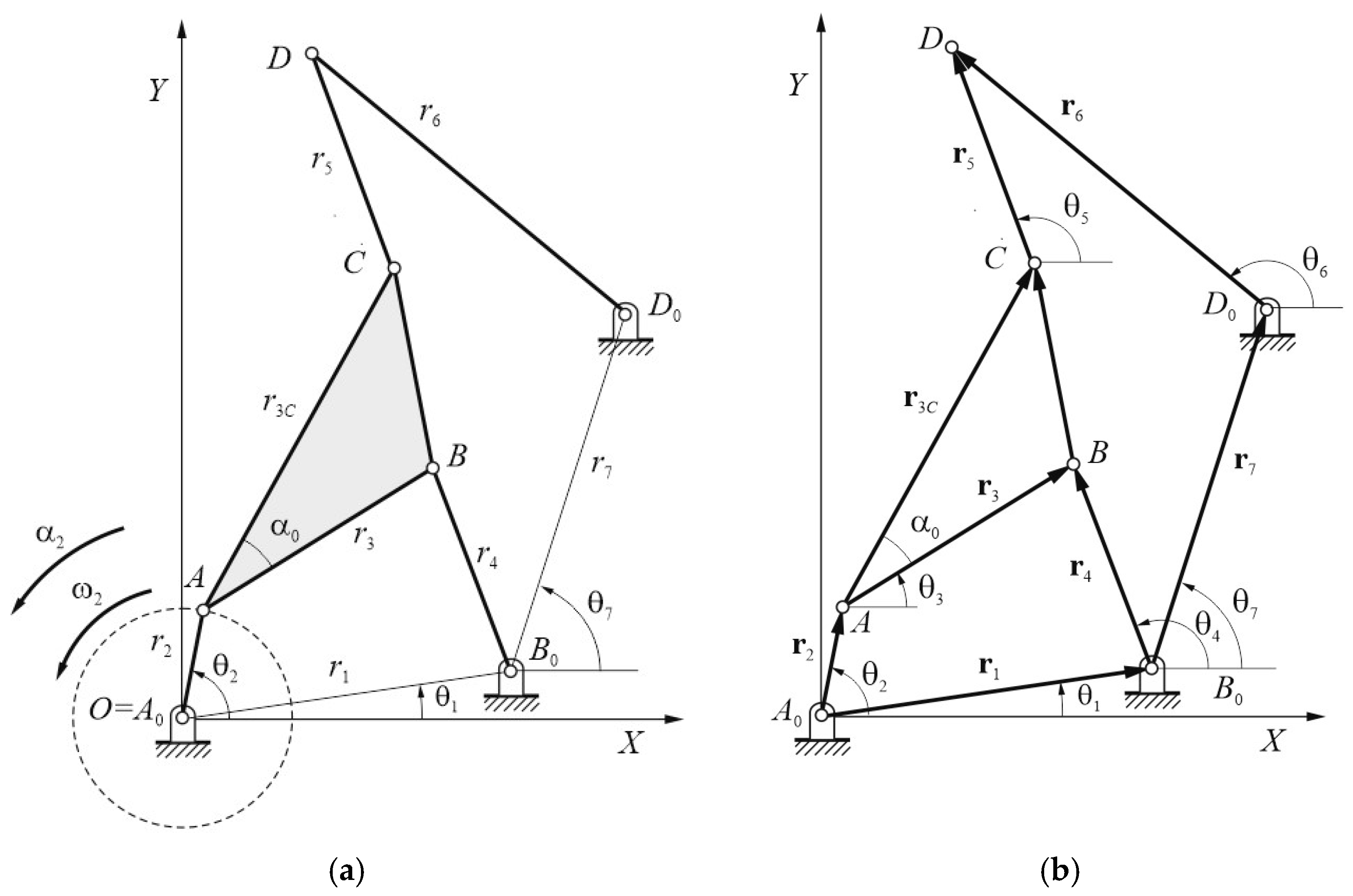
The Stephenson III six-bar mechanism is sketched in Figure 1a, composed of the four-bar linkage A0ABB0 and the CDD0 RR dyad, which are connected between them by means of the coupler triangle ABC. Link lengths are indicated with ri for i = from 1 to 7, along with the angles θ1 and θ7, which give the positions of r1 and r7, respectively, with respect to the positive X-axis of the OXY fixed reference frame. The relative position of point C with respect to the coupler link AB is given by the distance r3C and the angle α0. In general, the driving crank A0A rotates counterclockwise with angular position θ2, velocity ω2, and acceleration α2. Referring to the kinematic sketch of Figure 1b, where the fixed frame OXY has been chosen with O = A0, the position analysis of the Stephenson III six-bar mechanisms is formulated through the following two closed-loop equations:
where each vector ri for i = 1, …, 7 are expressed in Cartesian form as follows:
ri and θi are the magnitude and the counterclockwise oriented angles of ri, respectively, while r3C is the position vector of point C with respect to A. The unit vectors of the X and Y axes are i and j, respectively. Thus, substituting each vector ri of Equation (3) into Equation (1) and developing for the first loop of the four-bar linkage A0ABB0, one has the following:
where θ3 is the oriented angle of r3, θ1 of r1 is assigned, θ2 of r2 is the driving angle, while the output angle θ4 of r4 is given by the following:
which terms , , and take the following form:
and σ is equal to ±1 according to the corresponding assembly mode.

Figure 1.
Stephenson III six-bar mechanism: (a) kinematic sketch; (b) vector loops.
Thus, by determining the first-time derivatives of the X and Y scalar components of Equation (1), both angular velocity vectors ω3 and ω4 are obtained as a function of the given angular velocity ω2 of the driving crank 2:
where k is the unit vector of the Z-axis.
Similarly, by determining the second-time derivatives of the X and Y scalar components of Equation (1), both angular acceleration vectors α3 and α4 are obtained as a function of the given angular acceleration α2 of the driving crank 2:
The velocity vectors vA, vB, and vC of points A, B, and C, are obtained by developing the first-time derivatives of the following position vectors:
thus, obtaining the following:
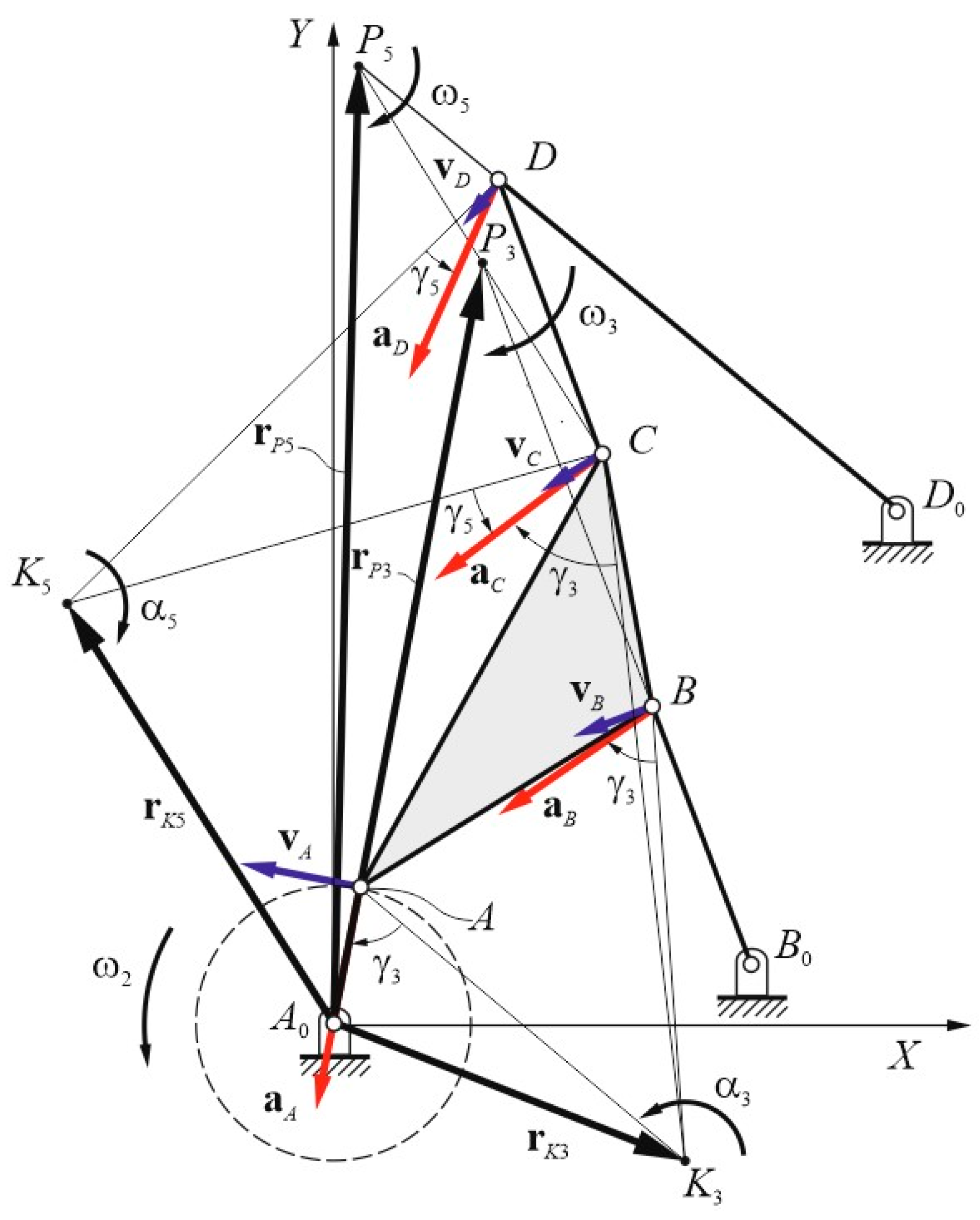
Referring to Figure 2, the position vector rP3 of the instantaneous center of rotation P3 of the coupler link AB is obtained by imposing a zero-velocity to P3, as follows:

Figure 2.
Velocity and acceleration vector fields.
Thus, substituting , , and , which are given by Equations (12) and (7), and by the first of Equation (11), into Equation (15) and developing, one has rP3 as follows:
The acceleration vectors aA, aB, and aC of points A, B, and C, are obtained by developing the second-time derivatives of the corresponding position vectors of Equation (1).
Therefore, one has the following:
The position vector rK3 of the acceleration center K3 of the coupler link AB is obtained by imposing a zero-acceleration to K3, as follows:
Thus, substituting , and , which are given by Equations (17) and (9), and by the first of Equation (11), into Equation (20), and developing, one has rk3 as follows:
Therefore, the position vectors rP3 and rK3 of the velocity and acceleration centers P3 and K3, which are sketched in Figure 2, are expressed in Cartesian form by Equations (16) and (21) and, with respect to the fixed frame OXY, as a function of the driving crank angle θ2.
Consequently, Equations (16) and (21) also represent the respective vector functions of the first- and second-order fixed centrodes of the coupler link AB (link 3).
Referring to Figure 1 and taking into account that we are dealing with Stephenson III six-bar mechanisms, the second closed-loop equation of Equation (2) must be developed.
Thus, substituting each vector ri in the Cartesian form of Equation (3) into Equation (2) and developing for the second loop of the five-bar linkage B0BCDD0, one has the following:
where , , and are given by the following:
and, in turn, one has the following:
The oriented angles θ5 and θ6 only depend on the driving crank angle θ2.
By determining the first-time derivatives of the X and Y scalar components of Equation (2) and developing them, the angular velocity vectors ω5 and ω6 are given by the following:
Likewise, by determining the second-time derivatives of the X and Y scalar components of Equation (2) and developing them, both angular acceleration vectors α5 and α6 are obtained as follows:
Moreover, the velocity vector vD of point D is obtained by developing the first-time derivative of the following position vector:
thus, obtaining the following:
Referring to Figure 2, the position vector rP5 of the instantaneous center of rotation P5 of the coupler link CD is obtained by imposing a zero-velocity to P5, as follows:
Thus, substituting , , and , which are given by Equations (14) and (25), and by the third part of Equation (11), into Equation (31), and developing, one has rP5 as follows:
The acceleration vector aD of point D is obtained by developing the second-time derivative of the corresponding position vector of Equation (2), by which one has the following:
The position vector rK5 of the acceleration center K5 of the coupler link CD is obtained by imposing a zero-acceleration to K5, as follows:
Thus, substituting , and , which are given by Equations (19) and (10), and by the third of Equation (11), into Equation (34), and developing, one has rk5 as follows:
Therefore, the position vectors rP5 and rK5 of the velocity and acceleration centers P5 and K5, which are sketched in Figure 2, are expressed in Cartesian form by Equations (32) and (35) and with respect to the fixed frame OXY, as a function of the driving crank angle θ2.
Consequently, Equations (32) and (35) also represent the respective vector functions of the first- and second-order fixed centrodes of the coupler link CD (link 5).
3. Bresse’s Circles
Bresse’s circles consist of the well-known inflection and stationarity circles, which intersect at both the instantaneous center of rotation P3 and the acceleration center K3. The inflection circle I3 is the geometric locus of all coupler points, which show an inflection point in their paths and I3 is always tangent to both centrodes at the P3 point. The stationarity circle S3 is the locus of all coupler points which show a pure normal acceleration.
Thus, both Bresse’s circles are now derived by using vector algebra, and, in particular, the equation of the inflection circle I3 is obtained as the locus of all the coupler points whose velocity and acceleration vectors are parallel to each other.
This condition can be expressed by imposing a zero-cross product, as follows:
where M3 is a generic coupler point of link 3. In particular, vectors and are obtained by Equations (13) and (18) for B = M3 and refer to the velocity and acceleration vectors of point A. Thus, substituting and from Equations (7) and (9) into Equations (13) and (18), one has and in matrix form, as follows:
where and , along with x and y, are the Cartesian components of and , respectively, and the symbol T indicates the transpose matrix.
Therefore, by substituting Equations (37) and (38) into Equation (36) and developing it, one has the following algebraic equation of the inflection circle I3:
the compact version of which is reported below:
where the following is true:
Likewise, the stationarity circle S3 is the geometric locus of all coupler points at which the velocity and acceleration vectors and are normal to each other, which means that their dot product equals zero, as follows:
Therefore, substituting Equations (37) and (38) into Equation (42), and developing it, one has the following algebraic equation of the stationarity circle S3:
the compact equation of which is reported below:
where the following is true:
The same approach is now applied to the second coupler link CD of the Stephenson III six-bar mechanism and, thus, for the inflection circle I5, one has the following:
where M5 is a generic coupler point of link 5 and, consequently, its velocity and acceleration vectors and can be derived by Equations (31) and (34) for M5 = P5 and M5 = K5, respectively, whose reference point is C. Thus, and are given in matrix form as follows:
where, in addition to the previous terms, and , along with x and y, are the Cartesian components and , respectively.
Therefore, by substituting Equations (47) and (48) into Equation (46) and developing it, one has the following algebraic equation of the inflection circle I5:
the compact form of which is reported below:
where the following is true:
Finally, the stationarity circle S5 is obtained by the following:
and, thus, by substituting Equations (47) and (48) into Equation (52), one has the following:
the compact equation of which is the following:
where the following is true:
Bresse’s circles of both coupler links AB and CD of the Stephenson III six-bar mechanism have been determined in algebraic form with respect to the fixed frame OXY by using vector algebra. In particular, the inflection circles I3 and I5, along with the stationarity circles S3 and S5, are given by Equations (40), (50), (44), and (54), respectively.
4. First- and Second-Order Centrodes
In general, the relative planar motion between two rigid bodies can be reproduced by the pure rolling of two curves that take the role of the first-order centrodes, which are traced by the instantaneous centers of rotation on their corresponding planes. If one of the two rigid bodies is fixed, a pair of first-order fixed and moving centrodes can be obtained.
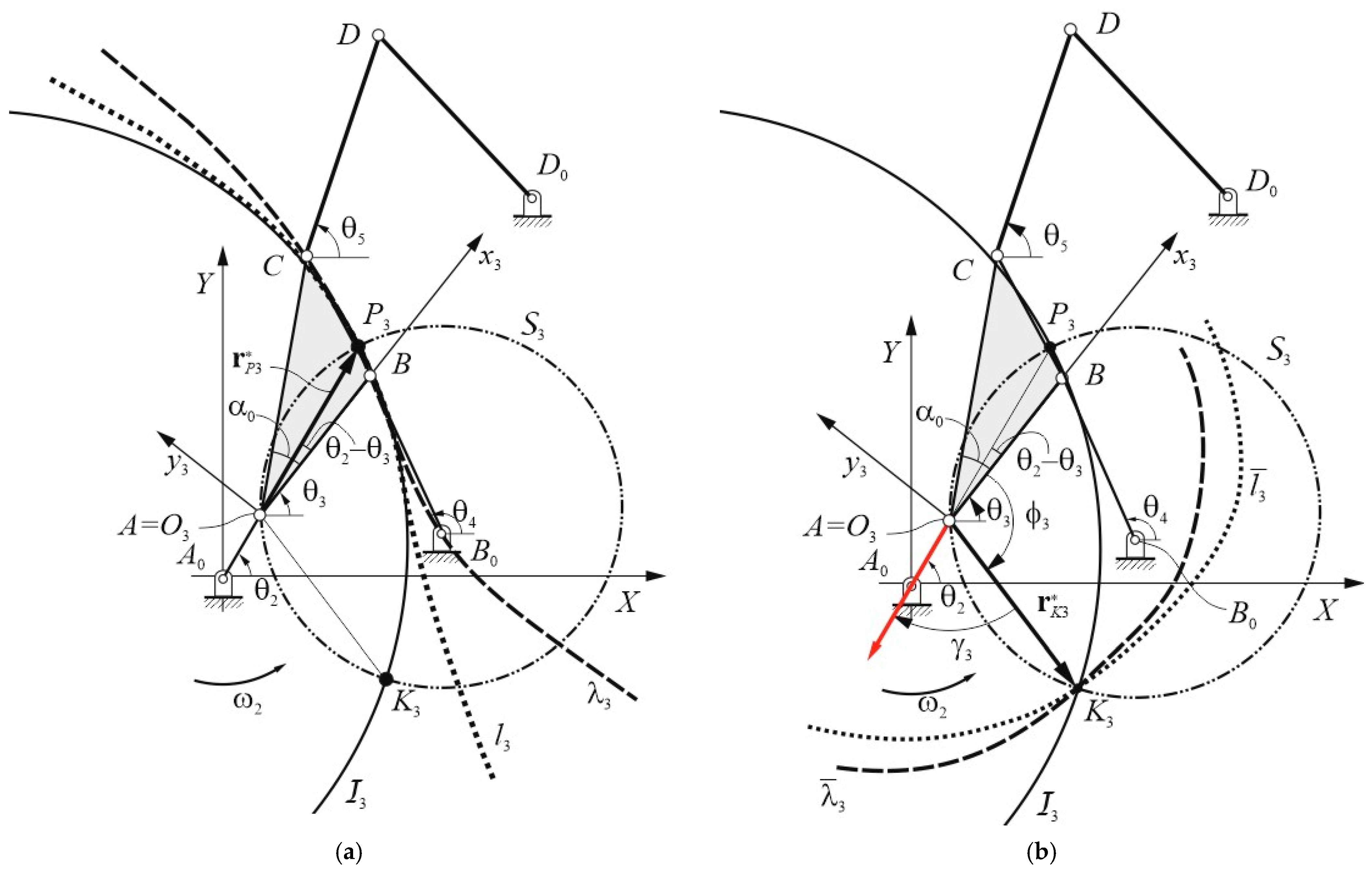
In particular, referring to Figure 3a, the fixed centrode λ3 is the path traced by the instantaneous center of rotation P3 of the coupler link 3 with respect to the fixed frame OXY, while the moving centrode l3 is the path traced by P3 with respect the moving frame O3×3y3 that is attached to AB (link 3).
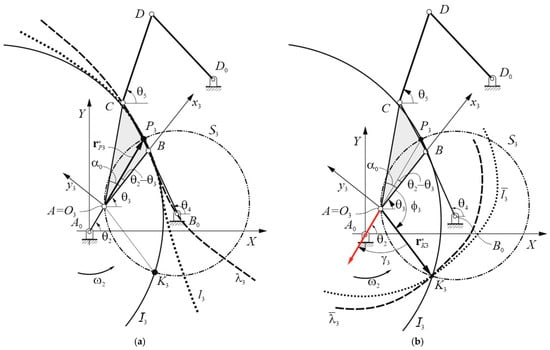
Figure 3.
Coupler link 3 (AB): (a) λ3 and l3; (b) and (the red arrow is aA).
Thus, the first-order fixed centrode λ3 of the coupler link 3 has been determined and expressed in Equation (16), while that of the corresponding moving centrode l3 is given by the following:
where is the position vector of P3 with respect to the moving frame O3x3y3.
Referring to Figure 3b, the second-order fixed centrode of the coupler link 3 has been determined previously and reported in Equation (21), while that of the second-order moving centrode is given as follows:
where is the position vector of K3 with respect to the moving frame O3x3y3, , , and .
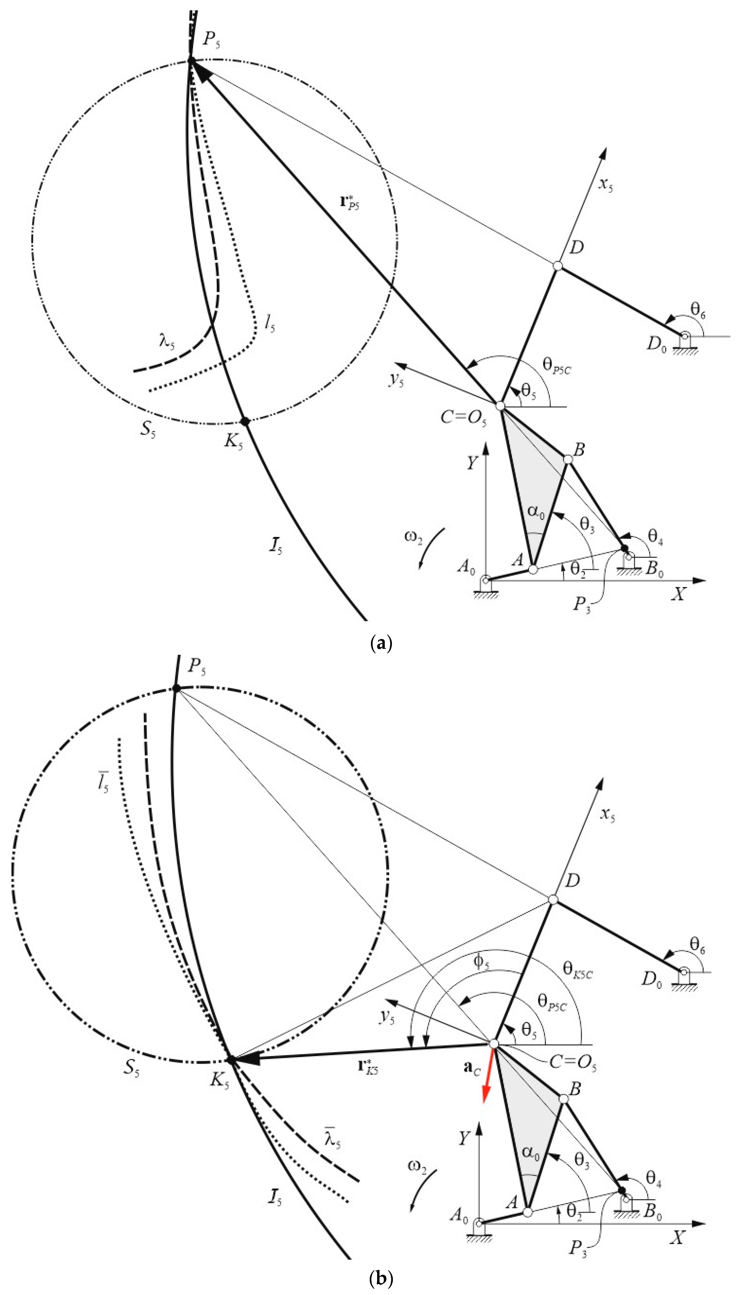
Similarly, referring to Figure 4a, the equation of the fixed centrode λ5 of the coupler link 5 has been determined in Equation (31), while that of the moving centrode l5 is given by the following:
where is the position vector of P5 with respect to the moving frame O5x5y5 and is its counterclockwise oriented angle, which is given by .
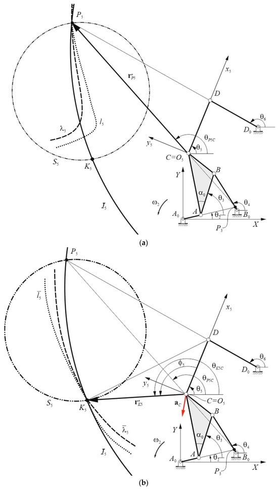
Figure 4.
Coupler link 5: (a) λ5 and l5; (b) and (the red arrow is aC).
Referring to Figure 4b, the second-order fixed centrode of the coupler link 5 has been determined and reported in Equation (34), while that of the second-order moving centrode takes the following form:
where is the position vector of K5 with respect to the moving frame O5x5y5, , , and .
Therefore, both pairs of moving centrodes, l3 and , along with l5 and , of the coupler links 3 and 5 are now expressed with respect to the fixed frame OXY by using the corresponding homogeneous transformation matrices, the general form of which is as follows:
where the subscript j has to be equal to 3 and 5 for the coupler links 3 and 5, respectively.
In fact, each moving centrode is attached to the corresponding coupler link and, thus, it performs a planar rigid-body motion which can be decomposed into a rotation and a translation, as Equation (60) does. Consequently, the equation of each moving centrode is transferred to the fixed frame by multiplying the corresponding homogeneous transformation matrix for Equations (56) and (58) of the first-order moving centrodes and for Equations (57) and (59) of the second-order moving centrodes, respectively.
5. Numerical Examples
The proposed formulation is general and, consequently, it could be implemented in any scientific software, such as Matlab, Maple, and Mathematica, or by using different Mathematical Programming Languages (MPLs), such as Python, C/C++, and Fortran. Nevertheless, considering the extended use of Matlab in many worldwide research centers and universities, as well as the availability of several specific tools for engineering applications and the possibility of coworking with other programming languages, the proposed formulation has been implemented in Matlab 2018 (release b) for validation, analysis, and design purposes by running several significant examples in different configurations.
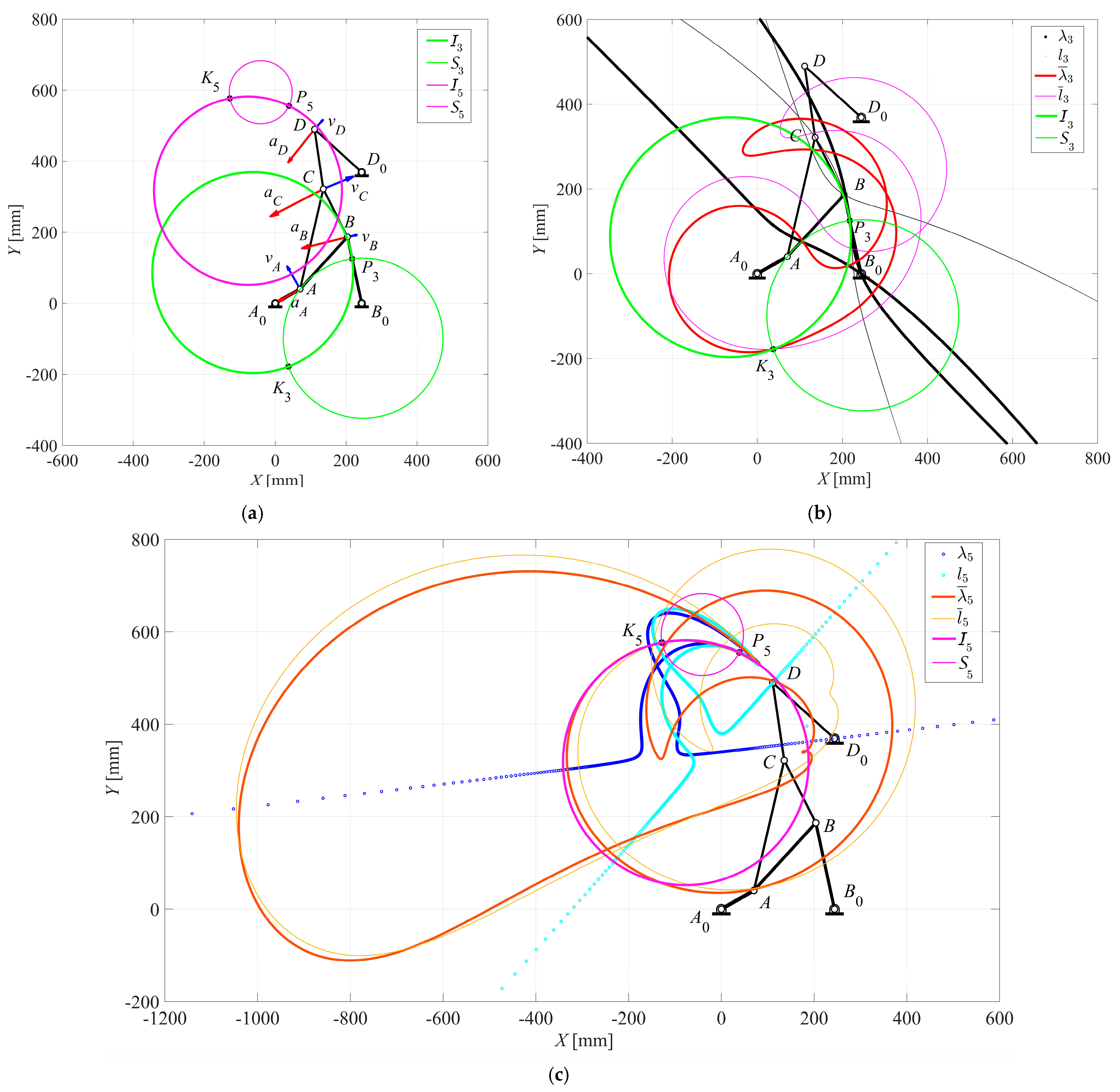
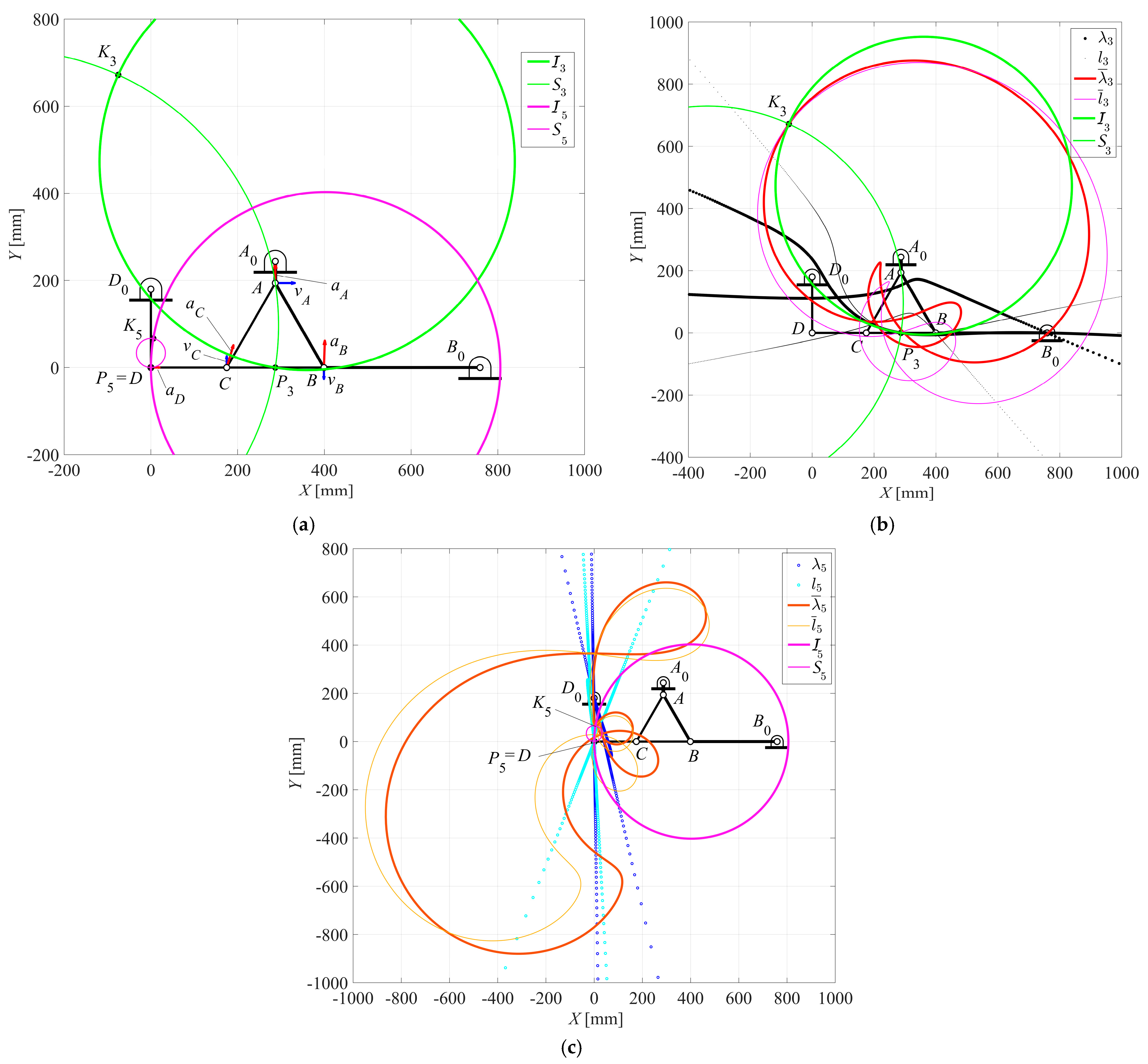
This is performed as shown in Figure 5 and for the following input data: ω2 = 1 rad/s, r1 = 244 mm, r2 = 81 mm, r3 = 198 mm, r3C = 288.9 mm, r4 = 191 mm, r5 = 170 mm, r6 = 180 mm, r7 = 369 mm, α0 = 29.32°, and θ2 = 25°.
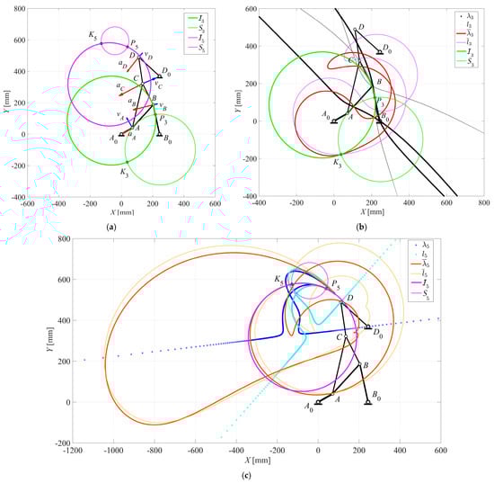
Figure 5.
Stephenson III six-bar mechanism for θ2 = 25°: (a) Bresse’s circles; (b) first-order centrodes and Bresse’s circles of link 3; (c) second-order centrodes and Bresse’s circles of link 5.
Figure 5a shows both pairs of Bresse’s circles, along with the velocity and acceleration vectors of the most significant mechanism points, by including both pairs of instantaneous centers of rotation P3 and P5, and the acceleration centers K3 and K5.
Figure 5b shows both the first- and second-order fixed and moving centrodes of the coupler link 3, along with the corresponding Bresse’s circles. Figure 5c shows both the first- and second-order fixed and moving centrodes of the coupler link 5, along with the corresponding Bresse’s circles.
The first-order centrodes are tangent to each other at the instantaneous center of rotation according to their pure-rolling motion, and they are also tangent to the corresponding inflection circle at the same point, while the second-order centrodes usually intersect with each other at more than one point and, of course, at the acceleration center.
Moreover, it is necessary to point out that the second-order centrodes are kinematic loci and not geometric loci, as the first-order centrodes, which depend on the kinematic input of the mechanism, that have been chosen in all the proposed examples have a constant driving angular velocity of ω2 = 1 rad/s.
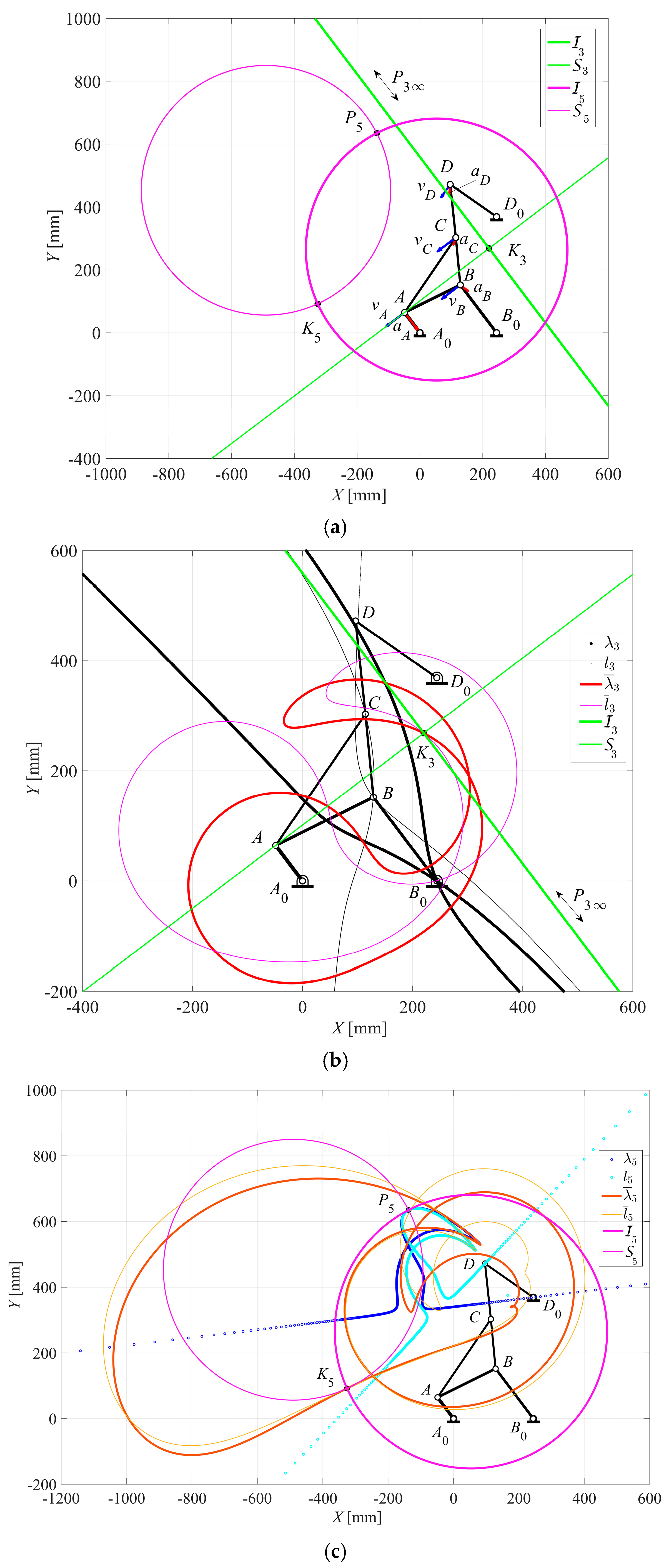
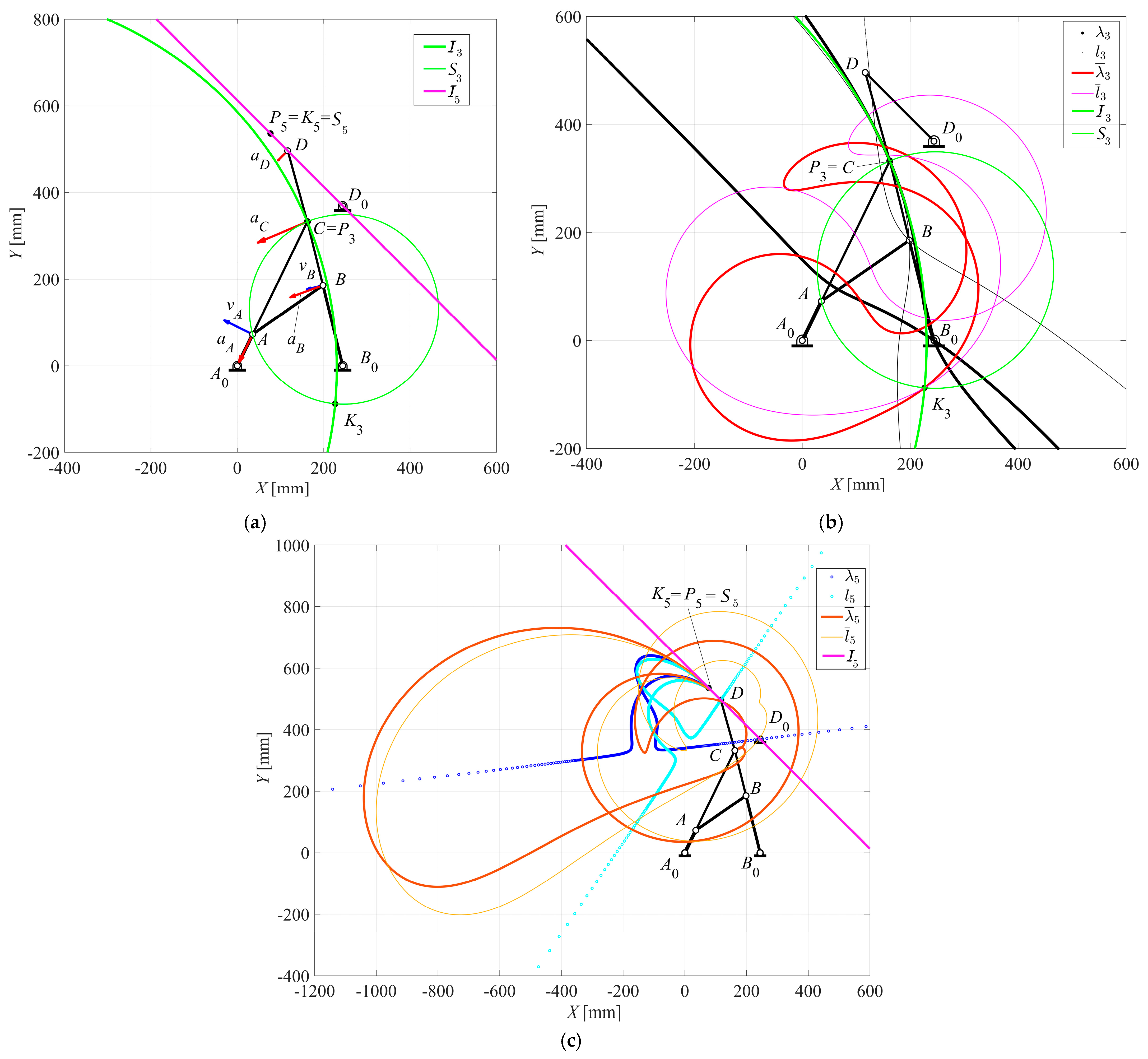
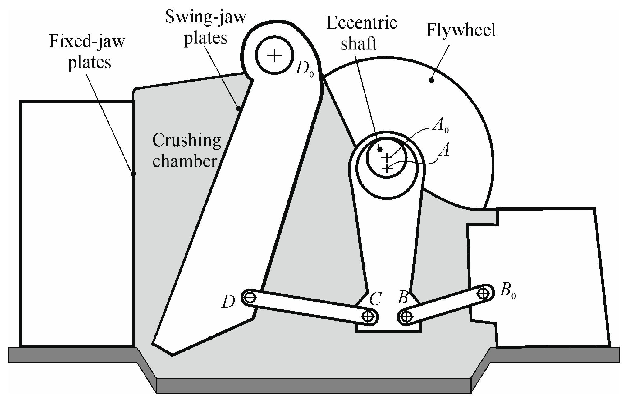
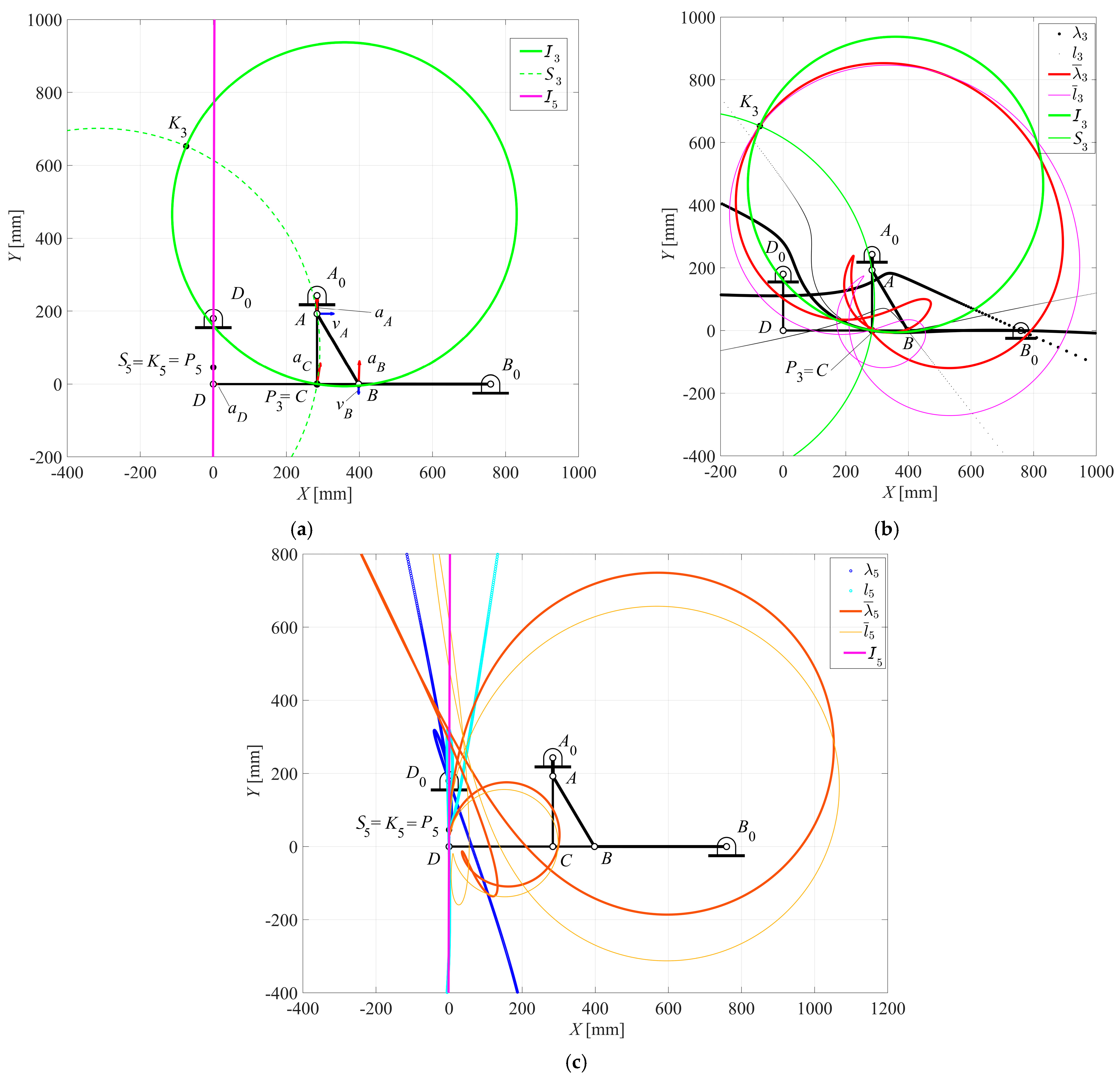
Similarly, Figure 6, Figure 7 and Figure 8 show the same mechanism in different configurations for the driving crank angle θ2 = 12.2°, θ2 = 127.15°, and θ2 = 64°, respectively. In particular, Figure 6a,b shows a case in which the stationarity circle degenerates into the straight line passing through the diameter of the inflection circle I3 at the P3 and K3 centers, and the line at infinity. Consequently, the acceleration center K3 coincides with the inflection pole and the second-order centrodes are tangent to each other at this point. Figure 6c shows the first- and second-order centrodes of the coupler link 5 in which the first-order centrodes are tangent to each other, as is typical, while the second-order centrodes intersect each other, including the acceleration center K5. Likewise, Figure 7 shows the particular case for which the instantaneous center of rotation P3 goes to infinity and both Bresse’s circles degenerate into two orthogonal lines, while Figure 8 reports the example in which the coupler link 5 is at the position of instantaneous stop, since not only the angular velocity ω5 is equal to zero, as when the instantaneous center of rotation goes to infinity, but also the velocity of any coupler point vanishes. However, the angular acceleration α5 is different from zero and the acceleration center K5 coincides with the instantaneous center of rotation P5. The stationarity circle degenerates into that point, while the inflection circle degenerates into the straight line passing through the points D0 and D (link 6) and the line at infinity. Moreover, a practical example regarding the jaw-crusher machine of Figure 9, as based on a Stephenson III six-bar mechanism, is developed and analyzed in both cases of simple dwell of the swing-jaw plate and the additional instantaneous stop of the second coupler link. In particular, this machine consists of the driving link A0A in the form of a suitable eccentric shaft that is attached to a flywheel, the four-bar linkage A0ABB0, and the five-bar linkage A0ACDD0, the output link D0D of which is the swing-aw plate, which crushes the stones against the corresponding fixed-jaw plate, as shown schematically in Figure 9. Thus, the Stephenson III six-bar mechanism of the jaw-crusher machine of Figure 9 is sketched as shown in Figure 10 and Figure 11, which refer to the case of simple dwell of the swing-jaw plate D0D and that of the additional instantaneous stop of the coupler link CD, respectively.
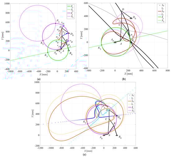
Figure 6.
Stephenson III six-bar mechanism for θ2 = 12.2°: (a) Bresse’s circles; (b) first-order centrodes and Bresse’s circles of link 3; (c) second-order centrodes and Bresse’s circles of link 5.
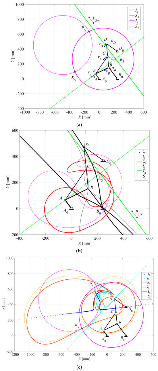
Figure 7.
Stephenson III six-bar mechanism for θ2 = 127.15°: (a) Bresse’s circles; (b) first-order centrodes and Bresse’s circles of link 3; (c) second-order centrodes and Bresse’s circles of link 5.
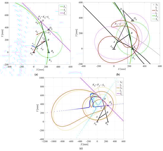
Figure 8.
Stephenson III six-bar mechanism for θ2 = 64°: (a) Bresse’s circles; (b) first-order centrodes and Bresse’s circles of link 3; (c) second-order centrodes and Bresse’s circles of link 5.
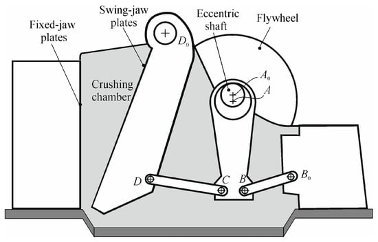
Figure 9.
Jaw-crusher machine.
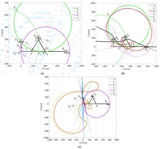
Figure 10.
Jaw-crusher machine at simple dwell configuration for θ2 = 270°: (a) Bresse’s circles; (b) first-order centrodes and Bresse’s circles of link 3; (c) second-order centrodes and Bresse’s circles of link 5.

Figure 11.
Jaw-crusher machine at dwell and instantaneous stop configuration for θ2 = 270°: (a) Bresse’s circles; (b) first-order centrodes and Bresse’s circles of link 3; (c) second-order centrodes and Bresse’s circles of link 5.
Consequently, the shape of the ternary coupler link ABC is assumed to have the form of an isosceles or right-angled triangle, respectively. In particular, as reported above in the previous examples, the Bresse circles, along with the velocity and acceleration vector fields, the first- and second-order centrodes of the coupler link 3, and finally, the same for the coupler link 5, are shown in Figure 10a and Figure 11a, Figure 10b and Figure 11b, and Figure 10c and Figure 11c, respectively.
In the case of Figure 10, for θ2 = 270°, the instantaneous center of rotation P5 coincides with D and is different from the acceleration center K5, with the swing-jaw plate having a zero angular velocity and, thus, a simple dwell, while Figure 11 shows the case of the instantaneous stop since both the coupler link CD and the swing-jaw plate D0D have velocities of zero.
In this particular configuration, for θ2 = 270°, the inflection circle I5 degenerates into the straight line passing through the points D0 and D, and the line at infinity; P3 coincides with C according to the design method proposed by the authors in [9], and P5 coincides with K5, while S5 degenerates into the same point.
The first- and second-order centrodes give useful information in terms of geometry and kinematics, about the planar motion of both pairs of points P3 and K3, along with P5 and K5.
6. Conclusions
The formulation of a general algorithm for obtaining the first- and second-order centrodes of both coupler links of Stephenson III six-bar mechanisms, along with the corresponding pairs of Bresse’s circles, has been proposed and validated by means of several significant examples. Particular attention has been devoted to the cases in which the second coupler link shows an instantaneous stop configuration, along with those where the first four-bar linkage reaches an asymptotic configuration. The obtained results can be useful to design and analyze specific mechanisms for practical applications, as well as those for obtaining dwell configurations of the output link or instantaneous stop configurations of the second coupler link. These kinematic performances can be required to design mechanisms for automatic machinery for the manufacturing industry, and a practical example regarding the jaw-crusher machine has been developed and analyzed.
Author Contributions
Conceptualization, G.F., C.L. and L.T.; methodology G.F., C.L. and L.T.; software, C.L.; validation, G.F., C.L. and L.T.; formal analysis, G.F and C.L.; investigation, G.F., C.L. and L.T.; resources, G.F. and L.T.; data curation, G.F., C.L. and L.T.; writing—original draft preparation, G.F., C.L. and L.T.; writing—review and editing, G.F., C.L. and L.T.; visualization, C.L. and L.T.; supervision, G.F.; project administration, G.F.; funding acquisition, G.F. All authors have read and agreed to the published version of the manuscript.
Funding
This research received no external funding.
Data Availability Statement
The original contributions presented in this study are included in the article. Further inquiries can be directed to the corresponding author.
Conflicts of Interest
The authors declare no conflicts of interest.
References
- Hartenberg, R.S.; Denavit, J. Kinematic Synthesis of Linkages; McGraw-Hill: New York, NY, USA, 1964. [Google Scholar]
- Hunt, K.H. Kinematic Geometry of Mechanisms; Clarendon Press: Oxford, UK, 1990. [Google Scholar]
- Pennestrì, E.; Cera, M. Engineering Kinematics: Curvature Theory of Plane Motion; Independently Published: Roma, Italy, 2023. [Google Scholar]
- Rosenauer, N.; Willis, A.H. Kinematics of Mechanisms; Dover: New York, NY, USA, 1967. [Google Scholar]
- Dijksman, E.A. Motion Geometry of Mechanisms; Cambridge University Press: Cambridge, UK, 1976. [Google Scholar]
- Chiang, C.H. Kinematics and Design of Planar Mechanisms; Krieger Publishing Company: Malabar, FL, USA, 2000. [Google Scholar]
- Hall, A.S., Jr. Kinematics and Linkage Design; Waveland Press: Prospect Heights, IL, USA, 1986. [Google Scholar]
- Figliolini, G.; Lanni, C.; Tomassi, L. First and Second Order Centrodes of Slider-Crank Mechanisms by Using Instantaneous Invariants. In Advances in Robot Kinematics: ARK 2022, 18th International Symposium on Advances in Robot Kinematics; Altuzarra, O., Kecskeméthy, A., Eds.; Springer: Cham, Switzerland, 2022; pp. 303–310. [Google Scholar]
- Figliolini, G.; Lanni, C.; Tomassi, L. Synthesis and Analysis of Stephenson III Six-Bar Motion Generators with an Instantaneous Stop Link. ASME. J. Mech. Robotics. 2025, 17, 044510. [Google Scholar] [CrossRef]
- Maleki, M.; Babahaji, A.; Mohtat, A. Further Analytical Investigation into Centrodes of the Planar FBL: Symbolic Representations, Double Points, Tacnodes, Degenerate Forms. Mech. Mach. Theory 2009, 44, 739–750. [Google Scholar] [CrossRef]
- Rosenauer, N. Acceleration Center Curves. Aust. J. Appl. Sci. 1954, 5, 103–115. [Google Scholar]
- Condurache, D. A Generalization of the Bresse Properties in Higher-Order Kinematics. In Advances in Robot Kinematics: ARK 2024; Lenarčič, J., Husty, M., Eds.; Springer: Cham, Switzerland, 2024. [Google Scholar]
- Condurache, D. Higher-Order Acceleration Center and Vector Invariants of Rigid Body Motion. In Proceedings of the 5th Joint International Conference on Multibody System Dynamics (MSD 2018), Lisbon, Portugal, 24–28 June 2018. Paper No. 160. [Google Scholar]
- Figliolini, G.; Lanni, C.; Cirelli, M.; Pennestrì, E. Kinematic Properties of nth-Order Bresse Circles Intersections for a Crank-Driven Rigid Body. Mech. Mach. Theory 2023, 190, 105445. [Google Scholar] [CrossRef]
- Bisshopp, K.E. Note on Acceleration in Laminar Motion. J. Mech. 1969, 4, 235–242. [Google Scholar] [CrossRef]
- Csernák, G. Analysis of Pole Acceleration in Spatial Motions by the Generalization of Pole Changing Velocity. Acta Mech. 2019, 230, 2607–2624. [Google Scholar] [CrossRef]
- Plecnik, M.M.; McCarthy, J.M. Kinematic Synthesis of Stephenson III Six-Bar Function Generators. Mech. Mach. Theory 2016, 97, 112–126. [Google Scholar] [CrossRef]
- Plecnik, M.M.; McCarthy, J.M. Design of Stephenson Linkages That Guide a Point Along a Specified Trajectory. Mech. Mach. Theory 2016, 96, 38–51. [Google Scholar] [CrossRef]
- Chakraborty, D.; Rathi, A.; Singh, R.; Pathak, V.K.; Srivastava, A.K.; Sharma, A.; Saxena, K.K.; Kumar, G.; Kumar, S. External Six-Bar Mechanism Rehabilitation Device for Index Finger: Development and Shape Synthesis. Robot. Auton. Syst. 2023, 161, 104336. [Google Scholar] [CrossRef]
- Baskar, A.; Plecnik, M. Synthesis of Six-Bar Timed Curve Generators of Stephenson-Type Using Random Monodromy Loops. ASME J. Mech. Robot. 2021, 13, 011005. [Google Scholar] [CrossRef]
- Tomassi, L.; Lanni, C.; Figliolini, G. A Novel Design Method of Four-Bar Linkages Mimicking the Human Knee Joint in the Sagittal Plane. In Advances in Italian Mechanism Science. IFToMM Italy 2022; Niola, V., Gasparetto, A., Quaglia, G., Carbone, G., Eds.; Mechanisms and Machine Science; Springer: Cham, Switzerland, 2022; Volume 122. [Google Scholar] [CrossRef]
- Diab, N. A New Graphical Technique for Acceleration Analysis of Four-Bar Mechanisms Using the Instantaneous Center of Zero Acceleration. SN Appl. Sci. 2021, 3, 327. [Google Scholar] [CrossRef]
- Hwang, W.M.; Fan, Y.S. Polynomial Equations for the Loci of the Acceleration Pole of a Slider-Crank Mechanism. Mech. Mach. Theory 2008, 43, 123–137. [Google Scholar] [CrossRef]
- Kulkarni, A.; Tesar, D. Properties of Higher Order Instant Center: A Case Study of Classical Motions. ASME J. Mech. Robot. 2013, 5, 024501. [Google Scholar] [CrossRef]
- Viaña, J.; Petuya, V. A Proposal for a Formula of Absolute Pole Velocities Between Relative Poles. Mech. Mach. Theory 2017, 114, 74–84. [Google Scholar] [CrossRef]
- Bottema, O. Acceleration Axes in Spherical Kinematics. ASME J. Eng. Ind. 1965, 87, 150–153. [Google Scholar] [CrossRef]
- Veldkamp, G.R. Acceleration Axes and Acceleration Distribution in Spatial Motion. ASME J. Eng. Ind. 1969, 91, 147–150. [Google Scholar] [CrossRef]
- Rico Martínez, J.M.; Duffy, J. Determination of the Acceleration Center of a Rigid Body in Spatial Motion. Eur. J. Mech. A/Solids 1998, 17, 969–977. [Google Scholar] [CrossRef]
- Mohamed, M.G. Kinematics of Rigid Bodies in General Spatial Motion: Second-Order Motion Properties. Appl. Math. Model. 1997, 21, 471–479. [Google Scholar] [CrossRef]
- Desai, J.P.; Žefran, M.; Kumar, V. A Geometric Approach to Second and Higher Order Kinematic Analysis. In Advances in Robot Kinematics: Analysis and Control; Lenarčič, J., Husty, M.L., Eds.; Springer: Dordrecht, The Netherlands, 1998. [Google Scholar] [CrossRef]
- Condurache, D. Higher-Order Kinematics of Rigid Bodies. A Tensors Algebra Approach. In Interdisciplinary Applications of Kinematics; Kecskeméthy, A., Geu Flores, F., Carrera, E., Elias, D., Eds.; Mechanisms and Machine Science; Springer: Cham, Switzerland, 2019; Volume 71. [Google Scholar]
- Condurache, D. Multidual Algebra and Higher-Order Kinematics. In New Trends in Mechanism and Machine Science: EuCoMeS 2020; Pisla, D., Corves, B., Vaida, C., Eds.; Springer: Cham, Switzerland, 2020. [Google Scholar] [CrossRef]
- Roth, B.; Yang, A.T. Application of Instantaneous Invariants to the Analysis and Synthesis of Mechanisms. ASME J. Eng. Ind. 1977, 99, 97–103. [Google Scholar] [CrossRef]
- Bottema, O. Some Remarks on Theoretical Kinematics: I Instantaneous Invariants; II On the Application of Elliptic Functions in Kinematics. In Proceedings of the International Conference for Teachers of Mechanisms, Yale University; The Shoe String Press: New Haven, CT, USA, 1961. [Google Scholar]
- Gazo-Hanna, E.; Saber, A.; Amine, S. Design and Modeling of a Six-Bar Mechanism for Repetitive Tasks with Symmetrical End-Effector Motion. Eng. Technol. Appl. Sci. Res. 2024, 14, 16302–16310. [Google Scholar] [CrossRef]
- Kapsalyamov, A.; Brown, N.A.T.; Goecke, R.; Jamwal, P.K.; Hussain, S. Velocity Control of a Stephenson III Six-Bar Linkage-Based Gait Rehabilitation Robot Using Deep Reinforcement Learning. Neural Comput. Appl. 2025. [Google Scholar] [CrossRef]

Disclaimer/Publisher’s Note: The statements, opinions and data contained in all publications are solely those of the individual author(s) and contributor(s) and not of MDPI and/or the editor(s). MDPI and/or the editor(s) disclaim responsibility for any injury to people or property resulting from any ideas, methods, instructions or products referred to in the content. |
© 2025 by the authors. Licensee MDPI, Basel, Switzerland. This article is an open access article distributed under the terms and conditions of the Creative Commons Attribution (CC BY) license (https://creativecommons.org/licenses/by/4.0/).