Time-Domain and Neural Network-Based Diagnosis of Bearing Faults in Induction Motors Under Variable Loads

Abstract

Bearing faults are the most common type of failure in induction motors, given their long operating times and mechanical loads. Because induction motors in industrial environments operate under various load conditions, effective methods for diagnosing bearing faults across these conditions have become increasingly important. Here, different load conditions were implemented with a powder clutch and a tension controller, and vibration data were acquired under both normal and faulty bearing conditions. To ensure diagnostic accuracy while improving time efficiency, a model bank-based fault diagnosis classifier is proposed, which utilizes independent classifiers trained for each load condition. For comparison, a single model-based classifier trained on all load conditions is also implemented. Both approaches are validated with three classifiers: support vector machine (SVM), multilayer neural network (MNN), and random forest (RF), with three input types: raw time-series signals, six statistical features, and three t-test–selected statistical features. Experimental results reveal that the model bank-based fault diagnosis classifier utilizing three statistical features selected by t-test maintained 98–100% accuracy while reducing operating time compared with Method 1 by 60.0, 71.2, and 60.0% for SVM, MNN, and RF, respectively. These results confirm that the proposed Method 2 utilizing time-domain analysis provides reliable and time-efficient performance for bearing fault diagnosis under variable load conditions.

1. Introduction

Induction motors are essential components in modern industry and are widely used across various fields due to their low cost and high efficiency [1,2]. However, with increasing use, they are exposed to extended operating times and mechanical loads, which increase fault frequency. This degradation reduces production efficiency and raises maintenance costs [3,4,5]. Faults in induction motors can be classified as electrical or mechanical faults. Electrical faults include overload, open circuit, and short circuit, while mechanical faults include bearing, rotor, and stator faults. Bearing-related faults account for approximately 51%, while stator winding faults represent about 16%, faults caused by external factors about 16%, rotor faults about 5%, and other faults about 12% [6,7]. Therefore, bearing fault diagnosis is a critical aspect of induction motor operation.

Various diagnostic techniques have been proposed, such as Motor Current Signature Analysis (MCSA), temperature monitoring, and acoustic signal analysis [8,9,10]. Of these, vibration analysis is the most widely applied method, since it can capture mechanical imbalance, impact, and resonance signals generated by faults [11,12]. Recent studies have adopted domain-based approaches to analyze vibration signals. For example, the Fast Fourier Transform converts time-domain signals into the frequency domain for analysis, and the Wavelet Transform provides time–frequency information to detect localized faults [13,14,15].

Furthermore, various analysis methods have been combined with machine learning to diagnose bearing faults [16,17,18,19]. Wang et al. [20] developed a wireless three-axis on-rotor sensing system that significantly improved the signal-to-noise ratio of vibration data and enabled accurate and robust detection of early outer- and inner-race bearing faults in induction motors through FFT and Hilbert envelope analysis. Qiu et al. [21] proposed a weak fault detection and extraction method based on Morlet wavelet filtering of vibration signals, demonstrating the potential for early prognostics. El Bouharrouti et al. [22] reduced vibration data from 48 kHz to 1 kHz using fractional downsampling at multiple sampling frequencies and applied the resampled data to SVM, MNLR, XGBoost, and LSTM classifiers. They successfully classified ten bearing fault conditions and analyzed the trade-off between sampling frequency and model performance. Sobie et al. [23] proposed a simulation-driven machine learning framework to address the shortage of real fault data. They generated synthetic vibration signals via high-resolution bearing dynamics simulations and applied angle synchronous averaging and envelope processing to remove geometry- and speed-dependent effects. Their approach combined CNN and nearest-neighbor dynamic time warping classifiers, revealing that models trained on simulated data could achieve high diagnostic accuracy when tested on experimental measurements. Matania et al. [24] introduced a hybrid zero-fault-shot learning algorithm that merges physics-based signal processing with neural networks. By augmenting training with both simulated and endurance test data, the method narrowed the simulation–reality gap and achieved over 98% accuracy across several bearing fault datasets. Snyder et al. [25] presented the dual-head ensemble transformer (DHET), which fuses a 1D transformer for raw vibration signals with a 2D vision transformer for STFT spectrograms within a dual time–frequency framework. The DHET attained 99.92% classification accuracy on the CWRU dataset and demonstrated superior robustness under varying load conditions compared to conventional CNN, RNN, and single transformer models.

However, despite these advances, little research has explored lightweight fault diagnosis methods that remain effective under variable load conditions while relying solely on time-domain information. Achieving lightweight and computational efficiency requires developing time-domain–based approaches and corresponding diagnostic frameworks that reduce complex signal processing.

This study presents an efficient and reliable bearing fault diagnosis method under variable load conditions by applying time-domain analysis, which eliminates complex signal processing while maintaining high diagnostic accuracy. The inputs include time-series signals without preprocessing, six time-domain statistical features (mean, variance, minimum, maximum, skewness, and kurtosis), and three key features (kurtosis, skewness, and maximum) selected through an independent t-test [26,27] for comparative analysis.

Various load conditions were simulated via a powder clutch, and four load levels (no load, 8 V, 16 V, and 24 V) were applied with a tension controller. Models trained under a single load cannot adequately capture the distributional differences under other load conditions. This limitation motivated the development of a model bank-based fault diagnosis classifier in which independent classifiers are trained and operated for each load condition. For comparison, a single model-based classifier trained on all load conditions was also implemented. Both approaches were assessed with support vector machine (SVM), multilayer neural network (MNN), and random forest (RF) algorithms to compare diagnostic performance. Here, the single model-based fault diagnosis classifier is referred to as Method 1, and the model bank-based fault diagnosis classifier as Method 2.

The objectives of this study are as follows:

• To demonstrate that bearing fault diagnosis under variable load conditions can be effectively performed in the time domain analysis, demonstrating that complex signal processing can be replaced.
• To verify that the machine learning algorithms of the proposed Method 2 enable accurate and rapid diagnosis under variable load conditions.

This paper is organized as follows. Section 2 discusses the theoretical background; Section 3 presents the proposed fault diagnosis algorithm; Section 4 describes the experimental setup and data acquisition; Section 5 discusses the results, and Section 6 concludes the study.

2. Theoretical Background

2.1. Statistical Features

In this study, six time-domain statistical features were calculated and used as feature vectors, as summarized in

Table 1. Statistical features used in this study.

Statistical Features	Equation
Mean	$\frac{1}{N}{\displaystyle \sum _{i=1}^N}{x}_i$
Variance	${\displaystyle \frac{1}{N}}{{\displaystyle \sum _{i=1}^N}(x_i-\mu )}^2$
Max	$\max \left(x_i\right)$
Min	$\min \left(x_i\right)$
Skewness	${\displaystyle \frac{1}{N}}{\displaystyle \sum _{i=1}^N}{\displaystyle \frac{{(x_i-\mu )}^3}{{\sigma }^3}}$
Kurtosis	${\displaystyle \frac{1}{N}}{\displaystyle \sum _{i=1}^N}{\displaystyle \frac{{(x_i-\mu )}^4}{{\sigma }^4}}$

[28,29,30]. The mean was obtained by summing all sample values and dividing by the number of samples, which represents the central tendency of the signal. The variance was determined by squaring the difference between each sample value and the mean, summing these values, and dividing by the total number of samples, which indicates the degree of dispersion around the mean. The maximum (Max) corresponds to the largest value within all observations and is useful for capturing transient high-amplitude vibrations. The minimum (Min) represents the smallest observed value. Skewness describes the asymmetry of a distribution by identifying whether extreme values are concentrated in one tail, thereby reflecting deviation from normality. Kurtosis was calculated in a similar way using the fourth power of the normalized deviation, and it indicates the sharpness and thickness of the distribution.

2.2. Independent t-Test

To assess the statistical significance of each time-domain feature between the normal and bearing-fault conditions, an independent t-test was applied. The t-test, a parametric statistical method, determines whether the mean difference between two independent groups is statistically significant. The resulting p-value indicates the strength of evidence against the null hypothesis, and a smaller p-value provides more substantial evidence that the two conditions differ, implying that the corresponding feature has higher discriminative capability for distinguishing fault conditions.

Here, the independent t-test was performed on six time-domain statistical features—mean, variance, maximum, minimum, skewness, and kurtosis. The p-values for all features were calculated, and the significance level was set to 0.05. Features for which the null hypothesis was rejected at this level were regarded as valid variables. Based on the t-test results shown in

Table 2. Results of the t-test.

Statistical Features	p-Value
Kurtosis	0
Skewness	$4.180\times {10}^{-159}$
Max	$1.306\times {10}^{-84}$
Min	$2.962\times {10}^{-24}$
Variance	$2.864\times {10}^{-4}$
Mean	$5.109\times {10}^{-2}$

, the mean did not reach statistical significance, whereas the remaining five features did. Among them, kurtosis, skewness, and maximum, which had the lowest p-values, were selected as input variables.

2.3. Support Vector Machine

SVM is a supervised learning-based classification algorithm that provides stable performance even with small datasets [31,32]. The objective of SVM is to find a hyperplane that best separates the data into their respective classes. The data points closest to this hyperplane are called support vectors, and the distance between the hyperplane and the support vectors is referred to as the margin [33]. The SVM structure is illustrated in Figure 1.

Given a training dataset ${\left\{\left(x_i, y_i\right)\right\}}_{i=1}^N$, where $x_i \in {\mathbb{R}}^d$ is the feature vector and $y_i \in \{ -1, +1 \}$ is the class label, the decision function of a linear SVM can be expressed as follows:

$$d\left(x\right)= {\omega }^{T}x+ b$$

(1)

Here, $\omega$ is the weight vector and $b$ denotes the bias term. SVM optimizes the hyperplane by maximizing the margin. However, in real-world scenarios, perfect linear separation of data is rarely possible. To address this, SVM introduces slack variables ${\xi }_i$ and a regularization parameter C. The optimization problem is formulated as follows:

$$\begin{gathered} \underset{\omega , b,\mathit{\xi }}{\min }{\displaystyle \frac{1}{2}}{‖\omega ‖}^2+ C\sum _{i=1}^N{\xi }_i \\ s.t. { y}_i\left({\omega }^T{x}_i+b\right)\ge 1- {\xi }_i, {\xi }_i\ge 0, i =1,\dots ,\mathrm{N} \end{gathered}$$

(2)

Here, ${\xi }_i$ represents the degree of margin violation for each instance, and C is a user-defined regularization parameter. A higher value of C reduces misclassification, making the SVM behave more like a hard-margin classifier, while a lower value of C allows more misclassifications and improves generalization.

2.4. Multilayer Neural Network

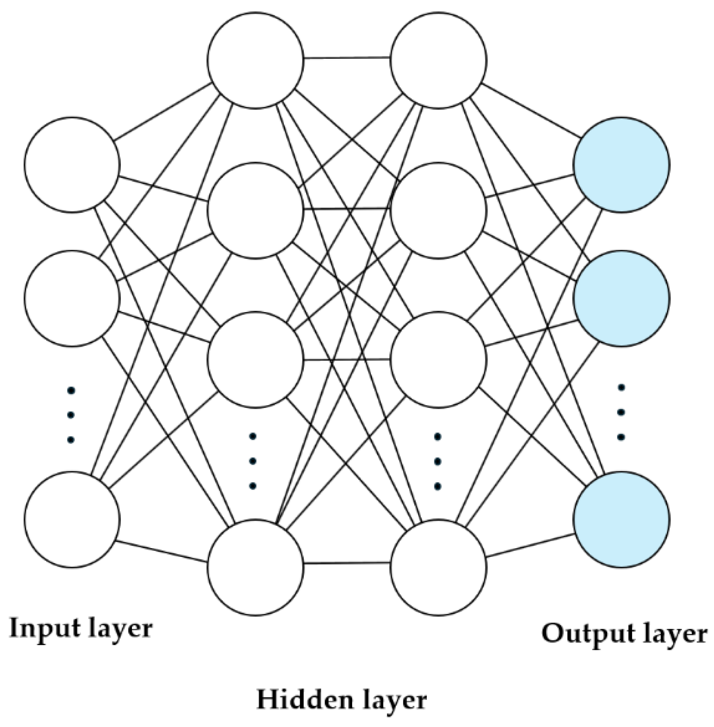
Figure 2 shows the structure of an MNN.

An MNN is a basic machine learning model that consists of an artificial neural network structure with multiple hidden layers placed between the input and output layers [34,35]. Each node receives the weighted sum of the outputs from the previous layer, together with a bias term, and produces the output through an activation function. This process is carried out via feedforward propagation:

$$h_j=f\left(\sum _i{w}_{ij}{h}_i+b_j\right)$$

(3)

Here, $h_j$ is the output of the node $j$ in the layer, $h_i$ denotes the output of the node $i$ in the previous layer. $w_{ij}$ represents the weight, $b_j$ is the bias, and $f\left(·\right)$ represents the activation function. During training, the difference between the predicted and actual values is calculated using a loss function, and the weights are updated through a backpropagation algorithm for optimization.

The MNN used in this study consists of an input layer, two hidden layers, and an output layer. The ReLU activation function [36] was used to alleviate the vanishing gradient problem. For the optimization algorithm, Adam [37] was used, which combines the RMSprop method and the Momentum method. The learning rate was set to 0.001, the default value suitable for the Adam algorithm.

2.5. Random Forest

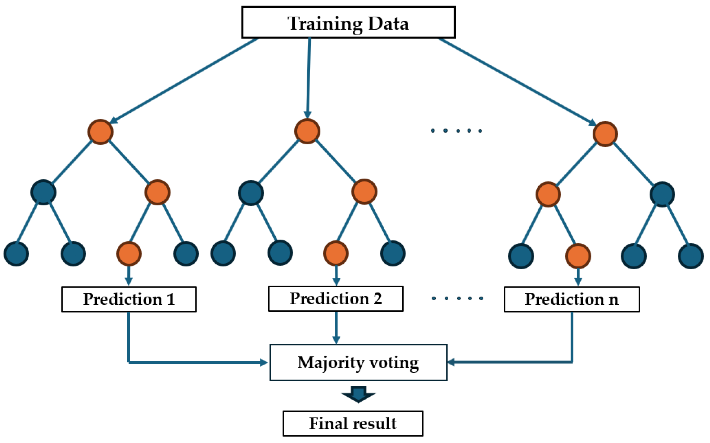
RF is an ensemble technique that combines multiple decision trees, and its structure is shown in Figure 3. Each tree is trained on individual samples generated through random bootstrap sampling from the original dataset, which ensures structural diversity. By aggregating a large number of such trees, RF achieves higher predictive stability than a single tree and reduces overfitting to the training data [38,39].

During the split process of each tree, only a subset of all available features is randomly selected and used, which lowers the correlation among trees and enhances predictive diversity, thereby improving the generalization performance of the model. The final output is obtained by aggregating the predictions of all trained trees: for classification tasks, the class chosen by the majority of trees is selected, whereas for regression tasks, the average of all predictions is used. In general, increasing the number of trees reduces prediction variance and stabilizes performance; however, beyond a certain threshold, the improvement becomes marginal relative to the computational cost. It is therefore important to determine an appropriate number of trees [40].

The main hyperparameters of the SVM, MNN, and RF used in this study are summarized in

Table 3. Model hyperparameter configuration.

Model	Input Data	Parameter	Value
SVM	Time series Statistical features	C	0.01
			0.1
MNN	Time series Statistical features	2 Hidden layers	128, 64
			64, 32
RF	Time series Statistical features	Number of trees	300
			100

. These hyperparameters were selected through a grid search process.

3. Proposed Fault Diagnosis Algorithm

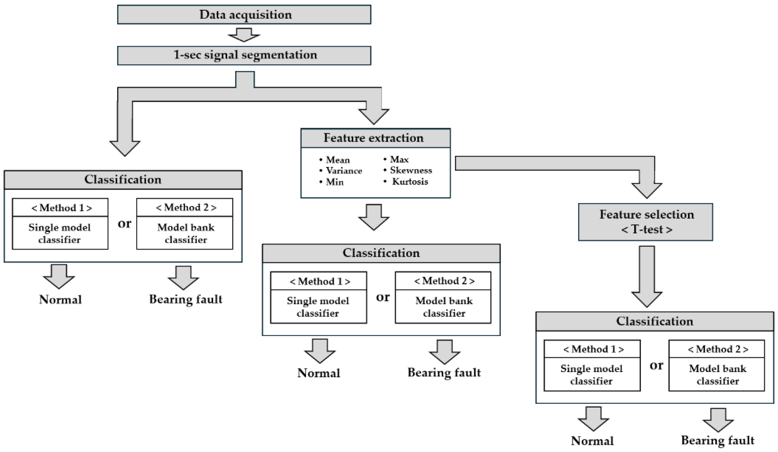
The induction motor fault diagnosis algorithm proposed in this study is illustrated in Figure 4. It consists of four main steps: data acquisition, signal segmentation, feature extraction, and classification.

• Data acquisition: Vibration signals were collected from induction motors under both normal and bearing fault conditions. The motor operated under four load levels: no load, 8 V, 16 V, and 24 V. Data were acquired using a vibration sensor with a sampling frequency of 1024 Hz.
• Signal segmentation: The acquired vibration signals were divided into 1 s segments to standardize the input length.
• Feature extraction: Three categories of input data were generated from the segmented signals. The first comprised time-series signals without preprocessing, and the second included statistical features, specifically the mean, variance, minimum, maximum, skewness, and kurtosis. The third utilized three statistically significant features—kurtosis, skewness, and maximum—selected from these six variables via an independent t-test.
• Classification: Two diagnostic methods were compared. Method 1 was trained using data from all load conditions with a single classifier, whereas Method 2 trained independent classifiers for each load condition to distinguish between normal and fault states. For fault classification, three models were employed (SVM, MNN, and RF).

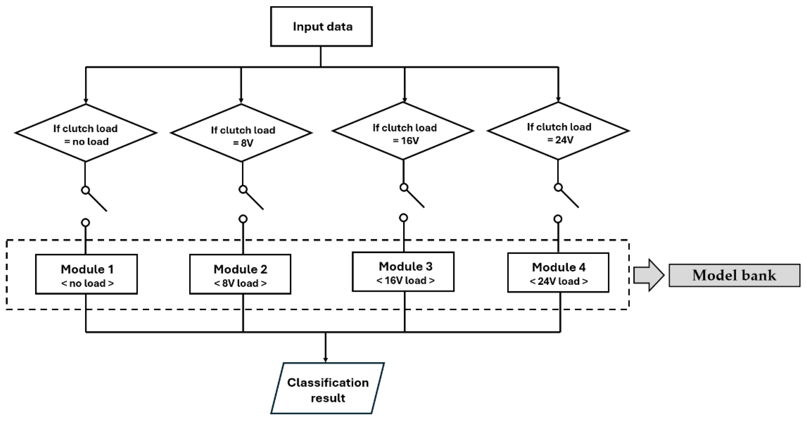
Figure 5 shows the proposed method (Method 2) in this study. Method 2 was evaluated under the assumption that the user has prior knowledge of the load condition applied to the induction motor. In this approach, an independent module trained on data corresponding to the specific load condition is selected based on the user-provided load information, and the input data are directed to this module for classification. The selected module then determines whether the input corresponds to a normal or bearing fault condition. This method improves diagnostic efficiency by using a classification model optimized for the signal distribution characteristics of each load condition, maintaining high diagnostic accuracy while improving computational efficiency.

4. Experimental Setup

4.1. Simulator Configuration

The configuration of the induction motor simulator is shown in Figure 6.

The simulator comprises the following components, as illustrated in Figure 6.

• Induction motor: Operated under both normal and bearing fault conditions; two identical motors were alternately installed for each condition.
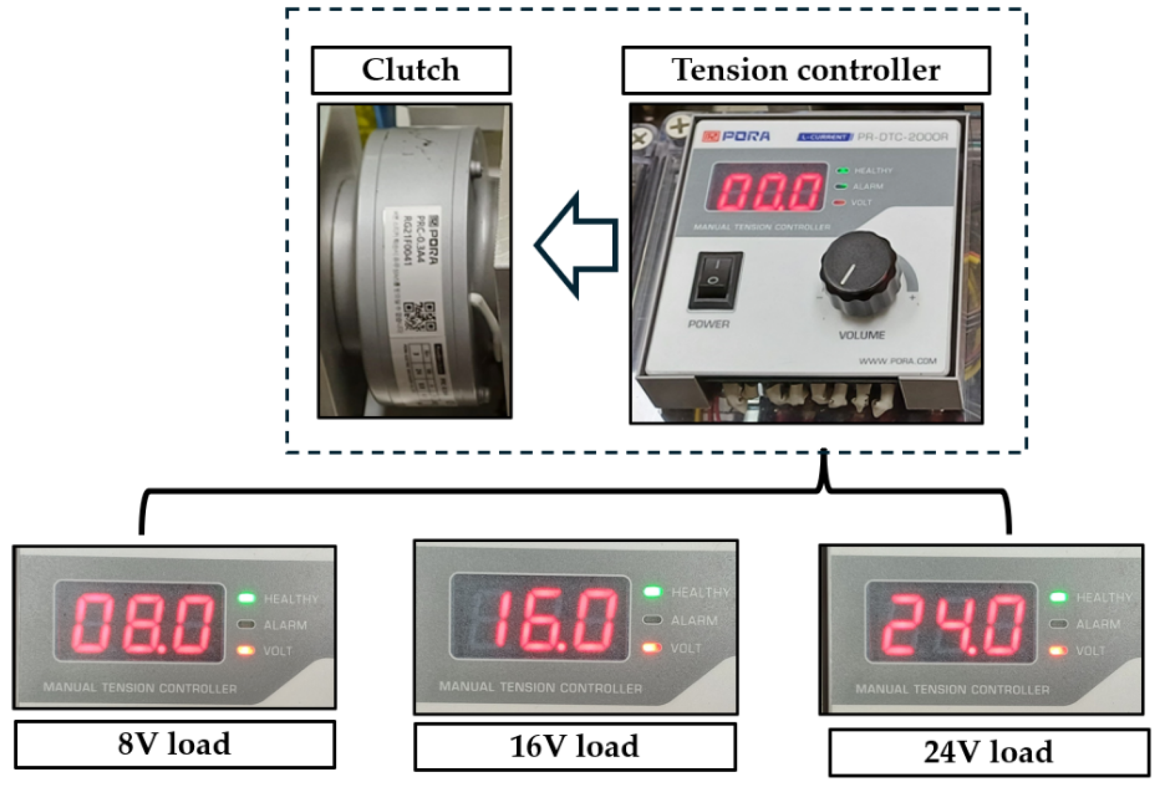
• Powder clutch and tension controller: Regulated the clutch torque to implement four load levels (no load, 8 V, 16 V, and 24 V).
• Inverter: Two inverters were utilized—one for the normal motor and another for the faulty motor—to maintain stable control.
• Vibration sensor: A 603C01 accelerometer (IMI Sensors, New York, NY, USA) mounted on the motor housing to capture vibration signals.
• Data acquisition module: NI-9234 (National Instruments, Austin, TX, USA) for signal recording at a sampling frequency of 1024 Hz.
• Control box: Integrated all power connections, the inverter control, and safety switches for system operation.

The specifications of the induction motor utilized here are provided in

Table 4. Induction motor specifications.

Parameter	Value	Parameter	Value
Rated power	0.2 kW	Rated torque	1.29/1.50 Nm
Rated voltage	220 V	Rated speed	1300/1550 rpm
Poles	4	Rated frequency	50/60 Hz

.

Power was supplied to the induction motor through the inverter, and the voltage was adjusted to 144 V to ensure stable operation of the engaged clutch. The powder clutch controlled the load using a tension controller, which implemented four load conditions: no load, 8 V, 16 V, and 24 V. Figure 7 shows the configuration used to apply the four load conditions through the tension controller.

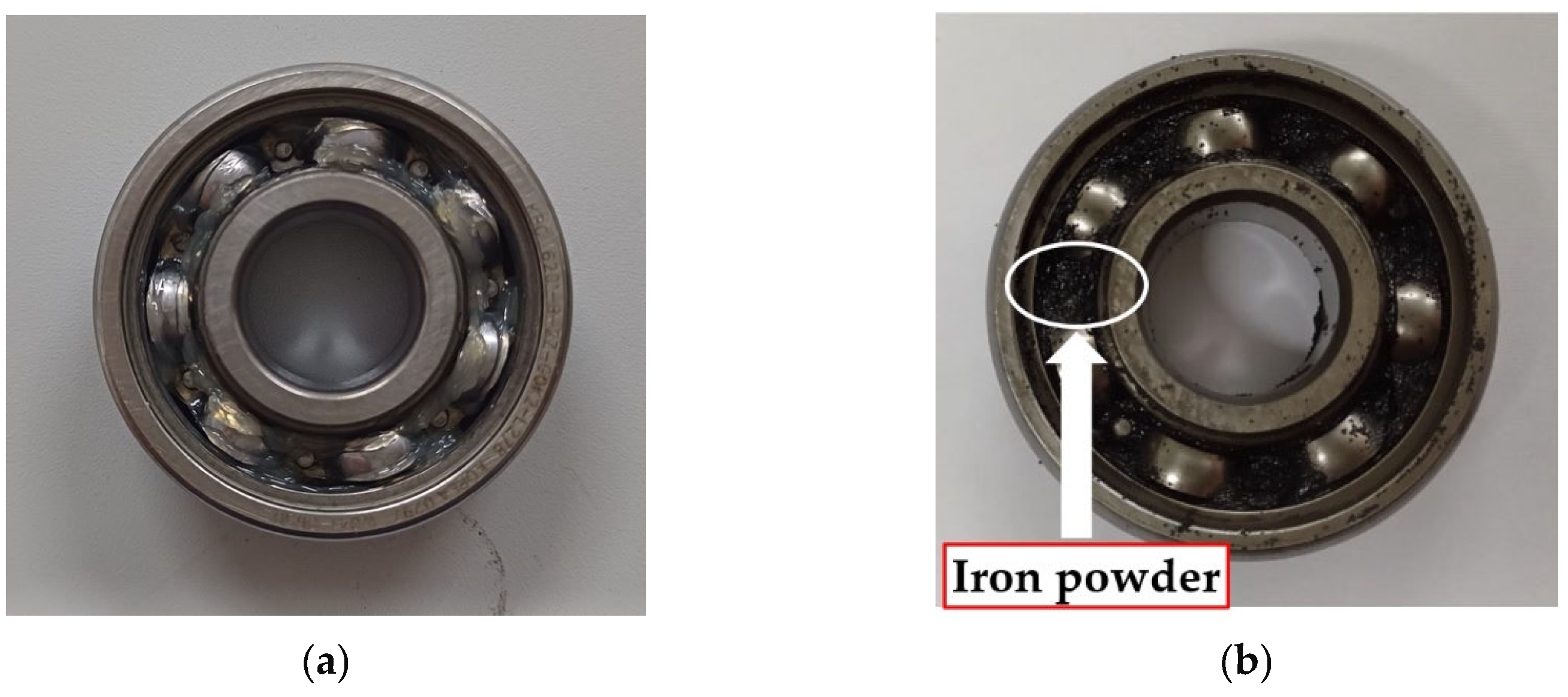
The bearing fault was induced by injecting iron powder into the bearing lubricant. The normal and fault conditions of the bearing are shown in Figure 8.

4.2. Data Acquisition

Vibration signals were measured at a sampling frequency of 1024 Hz using a 603C01 vibration sensor (IMI Sensors, New York, NY, USA) and an NI-9234 data acquisition module (National Instruments, Austin, TX, USA). The specifications of the vibration sensor used are listed in

Table 5. Vibration sensor specifications.

Parameter	Value
Measurement range	$490 \mathrm{m}/{\mathrm{s}}^2$
Frequency range	0.5 to 10,000 Hz
Transverse sensitivity	≤7%
Temperature range	−54 °C to 121 °C

.

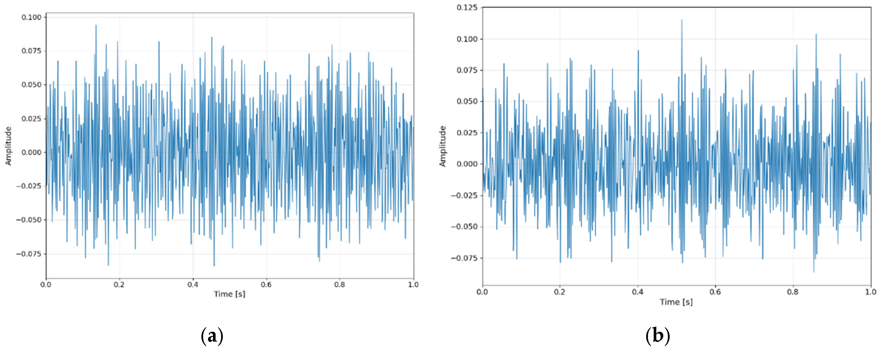
For each motor condition, vibration signals were collected for 180 s under four load levels (no load, 8 V, 16 V, 24 V). Data acquisition was repeated on two different days under identical experimental conditions to obtain two independent data groups. The first group was adopted as the training dataset, and the second group served as the test dataset. All vibration signals were divided into 1 s segments and treated as input data. Figure 9 presents examples of 1 s vibration signals under the 8 V load condition taken from the training dataset.

For each load condition, 360 datasets were obtained, comprising 180 normal and 180 bearing fault cases. Accordingly, 1440 datasets were collected per group. Hence, Method 1 utilized all load conditions, resulting in a total of 1440 training datasets and 1440 testing datasets. In contrast, Method 2 classified each load condition separately; therefore, each model bank was trained and tested with 360 datasets.

To eliminate scale differences and ensure stable training, z-score normalization was applied to all input data.

5. Results

5.1. Results of Method 1

Table 6. Accuracy and operating time of Method 1.

Model	Input Data	Accuracy (%)	Operating Time (s)
SVM	Time-series	51.7	0.50
	6 Statistical features	99.4	0.002
	3 Statistical features	99.7	0.002
MNN	Time-series	77.7	0.80
	6 Statistical features	99.0	0.59
	3 Statistical features	99.7	0.52
RF	Time-series	84.0	0.19
	6 Statistical features	99.6	0.02
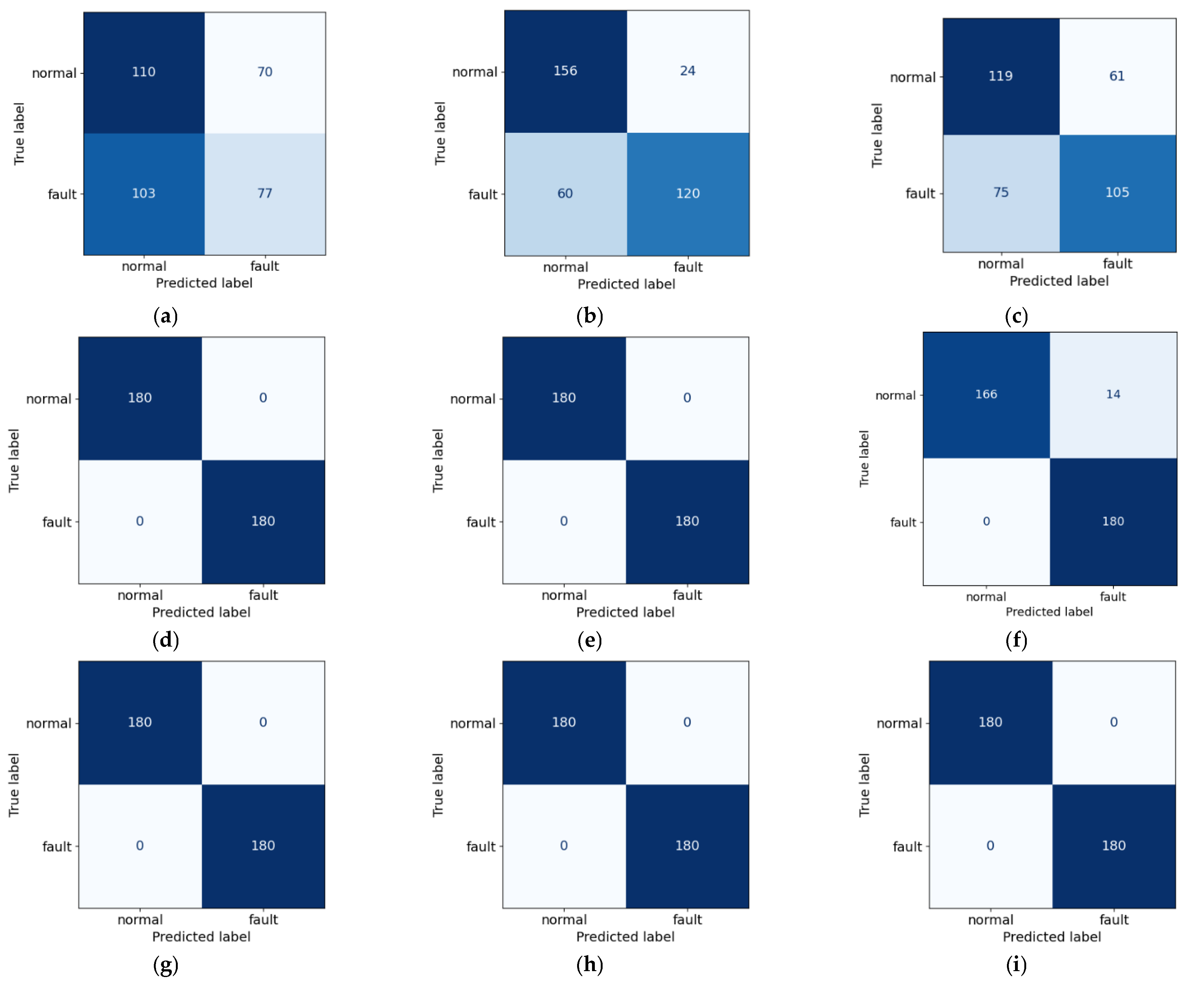
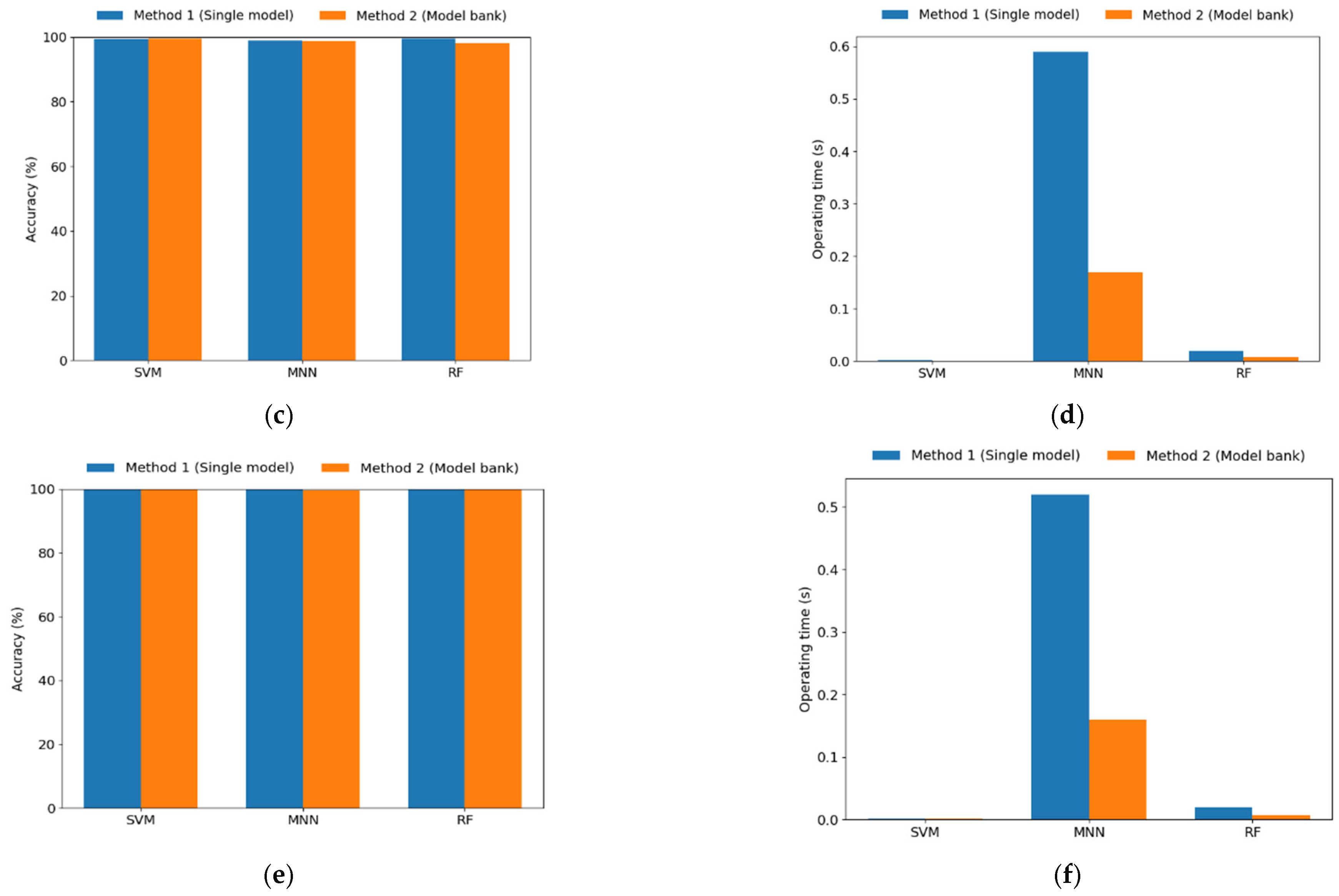
	3 Statistical features	99.7	0.02

summarizes the classification accuracy and operating time. With time-series input data, SVM achieved a low accuracy of 51.7%, while MNN and RF reached 77.7% and 84.0%. Although MNN and RF outperformed SVM, the improvement was limited, and the overall accuracy remained low. In contrast, when six statistical features were applied, SVM, MNN, and RF achieved 99.4%, 99.0%, and 99.6% accuracy, respectively. Restricting the input to the three most significant statistical features identified through the t-test increased accuracy to 99.7% across all models, indicating that selecting statistically significant features through the t-test improves diagnostic efficiency without compromising classification accuracy.

For the time-series input, the operating times were 0.50 s, 0.80 s, and 0.19 s for SVM, MNN, and RF, respectively. For the six-statistical-feature input, SVM achieved the fastest operation at 0.002 s (a 99.6% reduction), followed by RF at 0.02 s (89.5%), and MNN recorded 0.59 s (26.3%).

When utilizing the three statistical features selected through the t-test, the operating time was almost identical to that of the six-feature input.

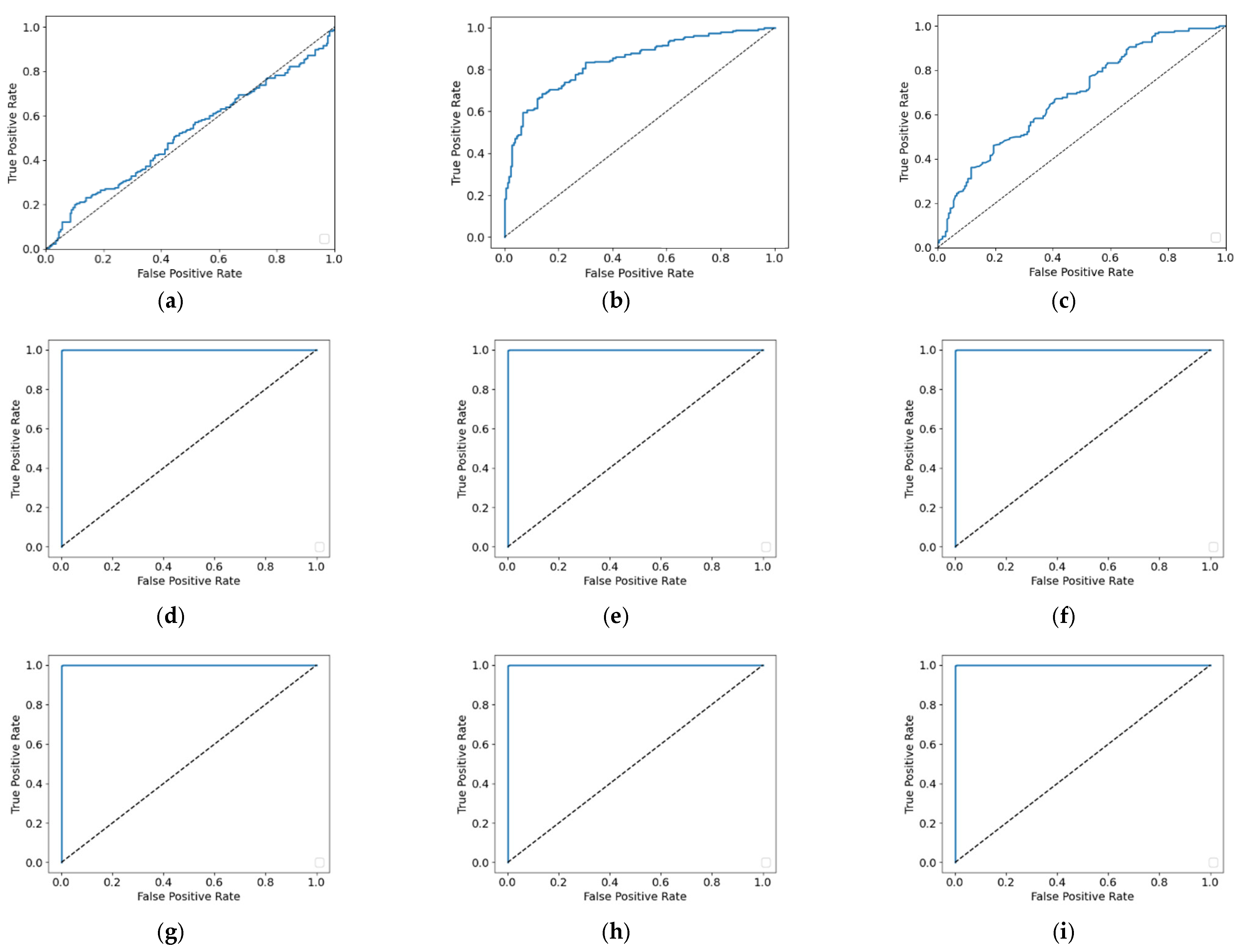
Figure 10 presents the confusion matrices, and Figure 11 illustrates the ROC curves of Method 1.

Hence, for Method 1, the statistical feature-based input was lighter and more effective. In addition, t-test–based selection of significant statistical features was found to improve classification accuracy, extracting essential characteristics for bearing fault classification compared with time-series inputs.

5.2. Results of Method 2

Table 7. Accuracy of Method 2.

Model	Input Data	Accuracy (%)
		Module 1 (No Load)	Module 2 (8 V Load)	Module 3 (16 V Load)	Module 4 (24 V Load)	Average
SVM	Time-series	53.3	51.9	55.6	52.5	53.3
	6-Statistical features	98.6	100.0	99.7	100.0	99.6
	3-Statistical features	98.9	100.0	100.0	100.0	99.7
MNN	Time-series	69.2	76.7	73.1	76.7	73.9
	6-Statistical features	95.0	100.0	99.7	100.0	98.7
	3-Statistical features	98.6	100.0	99.7	100.0	99.6
RF	Time-series	73.3	62.2	60.3	63.1	64.7
	6-Statistical features	98.3	96.1	98.3	99.7	98.1
	3-Statistical features	98.9	100.0	100.0	100.0	99.7

and

Table 8. Operating time of Method 2.

Model	Input Data	Operating Time (s)
		Module 1 (No Load)	Module 2 (8 V Load)	Module 3 (16 V Load)	Module 4 (24 V Load)	Average
SVM	Time-series	0.03	0.03	0.04	0.03	0.03
	6-Statistical features	0.0005	0.0009	0.0009	0.0009	0.0008
	3-Statistical features	0.0005	0.001	0.001	0.001	0.0009
MNN	Time-series	0.26	0.21	0.19	0.19	0.21
	6-Statistical features	0.21	0.14	0.15	0.18	0.17
	3-Statistical features	0.16	0.16	0.17	0.14	0.16
RF	Time-series	0.03	0.03	0.03	0.02	0.03
	6-Statistical features	0.008	0.009	0.009	0.007	0.008
	3-Statistical features	0.008	0.008	0.001	0.009	0.007

summarize the accuracy and operating time of Method 2 across all load conditions. With time-series input, Method 2 exhibited relatively low accuracy: SVM achieved 51.9–55.6% (53.3% on average), MNN achieved 69.2–76.7% (73.9% on average), and RF achieved 60.3–73.3% (64.7% on average). In contrast, with 6 statistical features as input, SVM achieved 100% accuracy under all load conditions except for Module 1 (no load, 98.6%) and Module 3 (16 V load, 99.7%). When the three selected statistical features were utilized, SVM improved from 98.6% to 98.9% at Module 1 and from 99.7% to 100.0% at Module 3 (16 V load). Similarly, MNN utilizing six statistical features achieved 100% accuracy except for Module 1 (no load) and Module 3 (16 V load), where it achieved 95.0% and 99.7%. When the three selected statistical features were utilized, MNN improved from 95.0% to 98.6% at Module 1. RF with six statistical features achieved 96.1–99.7% accuracy across all load conditions (98.1% on average), performing slightly lower than SVM and MNN. However, when the three selected statistical features were utilized, RF achieved 98.9% at Module 1 (no load) and 100% under the other load conditions.

Compared with the time-series input, the statistical feature-based input reduced the operating time by approximately 97.3% for SVM (0.03 s to 0.0008 s), 19.0% for MNN (0.21 s to 0.17 s), and 73.3% for RF (0.03 s to 0.008 s). Moreover, compared with the six-statistical-feature-based Method 1, Method 2 reduced the average operating time by approximately 60.0% for SVM (0.002 s to 0.0008 s), 71.2% for MNN (0.59 s to 0.17 s), and 60.0% for RF (0.02 s to 0.008 s). The three-statistical-feature input produced nearly the same operating time as the six-feature input.

The results confirm that Method 2 maintained high diagnostic accuracy and a shorter operating time than Method 1, and that feature selection remained effective in improving overall diagnostic performance.

Figure 12 presents the confusion matrices, and Figure 13 illustrates the ROC curves of Method 2 under the 8 V load condition.

Figure 14 shows a summary of the performance differences between Method 1 and Method 2.

6. Conclusions

This study proposed two approaches for effective diagnosis of bearing faults in induction motors under various load conditions. First, the effect of input type in the time domain was analyzed by comparing time-series signals, six statistical features, and t-test–based feature-selected inputs (kurtosis, skewness, and maximum). Second, Method 1 and the proposed Method 2 were compared to identify the optimal model structure for bearing fault diagnosis under variable loads. Fault diagnosis was performed using three classifiers—SVM, MNN, and RF—and the evaluation was based on classification accuracy and operating time.

To implement the various load conditions, a tension controller and a powder clutch were used. The induction motor was operated under four load levels: no load, 8 V, 16 V, and 24 V. An induction motor simulator incorporating both normal and faulty bearing states was constructed to acquire vibration data, which were collected on different days under identical experimental settings.

For Method 1 with time-series input, SVM, MNN, and RF achieved accuracies of 51.7%, 77.7%, and 84.0%, respectively, indicating low performance. In contrast, when six statistical features were adopted as input, SVM, MNN, and RF achieved 99.4%, 99.0%, and 99.6% accuracy, respectively. In addition, when three statistical features selected through the t-test were utilized, all three models achieved 99.7% accuracy. Regarding operating time, the 6-statistical-feature input also outperformed the time-series input, reducing operating time by approximately 99.6% for SVM (0.50 s to 0.002 s), 26.3% for MNN (0.80 s to 0.59 s), and 89.5% for RF (0.19 s to 0.02 s). The operating time of the three statistical features was similar to that of the six statistical features.

For Method 2, the time-series input produced low accuracy: SVM achieved 51.9–55.6% (53.3% on average), MNN achieved 69.2–76.7% (73.9% on average), and RF achieved 60.3–73.3% (64.7% on average). In contrast, the six-statistical-feature input yielded high accuracy, with SVM achieving 100% under all load conditions except for Module 1 (no-load, 98.6%) and Module 3 (16 V load, 99.7%). Similarly, MNN achieved 100% accuracy except for Module 1 (95.0%) and Module 3 (99.7%). RF recorded a slightly lower performance than SVM and MNN, recording accuracies of 96.1–99.7% across all load conditions. When three statistical features selected through the t-test were utilized, SVM improved to 98.9% at Module 1 and reached 100% at Module 3. MNN also improved to 98.6% at Module 1. In the case of RF, which had exhibited relatively lower performance, the accuracy increased to 98.9% at Module 1 and reached 100% under all other load conditions, demonstrating a noticeable improvement.

In terms of operating time, the statistical feature–based SVM in Method 2 recorded 0.0005–0.0009 s (0.0008 s on average), corresponding to an approximately 60.0% reduction compared with Method 1. MNN achieved 0.14–0.21 s (0.17 s on average), representing a reduction rate of about 71.2%. In the case of RF, 0.007–0.009 s (0.008 s on average) was observed, resulting in a reduction rate of about 60.0%. The operating time utilizing the three selected statistical features was almost identical to that of the six-feature input. These findings indicate that Method 2 effectively reduces operating time while maintaining high diagnostic accuracy.

In conclusion, Method 2 achieved diagnostic performance comparable to Method 1 while offering significantly shorter operating times. Moreover, the statistical feature-based input provided higher accuracy and shorter operating time than the time-series input across all diagnostic models. Selecting three statistical features that most strongly correlated with faults through the t-test was found to be effective, improving overall diagnostic performance. This demonstrated the importance of distinguishing between effective and ineffective statistical features in classification.

These results demonstrate that bearing faults can be effectively diagnosed under variable load conditions via time-domain analysis without a complex computational process. This approach validates its applicability to industrial environments where rapid fault detection and real-time decision-making are essential by minimizing model size and computational demand without compromising diagnostic performance.

This study is limited by its focus on bearing faults and the absence of noise commonly found in industrial settings. Future studies will extend experiments to include eccentricity and stator winding faults while introducing various types of noise—including Gaussian and nonperiodic impulsive noise—to reproduce realistic industrial conditions. Moreover, the proposed time-domain–based method will be further evaluated and compared with frequency- and time–frequency-domain techniques such as FFT and wavelet transform under these complex and noisy conditions.

References

1. Irfan, M.; Alwadie, A.S.; Glowacz, A.; Awais, M.; Rahman, S.; Khan, M.K.A.; Jalalah, M.; Alshorman, O.; Caesarendra, W. A Novel Feature Extraction and Fault Detection Technique for the Intelligent Fault Identification of Water Pump Bearings. Sensors 2021, 21, 4225. [Google Scholar] [CrossRef]
2. Zhen, D.; Wang, T.; Gu, F.; Ball, A.D. Fault Diagnosis of Motor Drives Using Stator Current Signal Analysis Based on Dynamic Time Warping. Mech. Syst. Signal Process. 2013, 34, 191–202. [Google Scholar] [CrossRef]
3. Kumar, R.R.; Andriollo, M.; Cirrincione, G.; Cirrincione, M.; Tortella, A. A Comprehensive Review of Conventional and Intelligence-Based Approaches for the Fault Diagnosis and Condition Monitoring of Induction Motors. Energies 2022, 15, 8938. [Google Scholar] [CrossRef]
4. Zamudio-Ramírez, I.; Osornio-Ríos, R.A.; Antonino-Daviu, J.A.; Quijano-Lopez, A. Smart-Sensor for the Automatic Detection of Electromechanical Faults in Induction Motors Based on the Transient Stray Flux Analysis. Sensors 2020, 20, 1477. [Google Scholar] [CrossRef] [PubMed]
5. Zarei, J. Induction Motors Bearing Fault Detection Using Pattern Recognition Techniques. Expert Syst. Appl. 2012, 39, 68–73. [Google Scholar] [CrossRef]
6. Gundewar, S.K.; Kane, P.V. Condition Monitoring and Fault Diagnosis of Induction Motor. J. Vib. Eng. Technol. 2021, 9, 643–674. [Google Scholar] [CrossRef]
7. Ruiz-Sarrio, J.E.; Antonino-Daviu, J.A.; Martis, C. Localized Bearing Fault Analysis for Different Induction Machine Start-Up Modes via Vibration Time–Frequency Envelope Spectrum. Sensors 2024, 24, 6935. [Google Scholar] [CrossRef]
8. Terron-Santiago, C.; Martinez-Roman, J.; Puche-Panadero, R.; Sapena-Bano, A. A Review of Techniques Used for Induction Machine Fault Modelling. Sensors 2021, 21, 4855. [Google Scholar] [CrossRef]
9. Xu, L.; Teoh, S.S.; Ibrahim, H. A Deep Learning Approach for Electric Motor Fault Diagnosis Based on Modified InceptionV3. Sci. Rep. 2024, 14, 12344. [Google Scholar] [CrossRef]
10. Lucas, G.; de Castro, B.; Serni, P.; Riehl, R.; Andreoli, A. Sensors Applied to Bearing Fault Detection in Three-Phase Induction Motors. Eng. Proc. 2021, 10, 40. [Google Scholar] [CrossRef]
11. Gangsar, P.; Tiwari, R. Comparative Investigation of Vibration and Current Monitoring for Prediction of Mechanical and Electrical Faults in Induction Motor Based on Multiclass-Support Vector Machine Algorithms. Mech. Syst. Signal Process. 2017, 94, 464–481. [Google Scholar] [CrossRef]
12. Łuczak, D. Machine Fault Diagnosis through Vibration Analysis: Continuous Wavelet Transform with Complex Morlet Wavelet and Time–Frequency RGB Image Recognition via Convolutional Neural Network. Electronics 2024, 13, 452. [Google Scholar] [CrossRef]
13. Yoo, S.M.; Lee, H.G.; Hao, W.K.; Lee, I.S. Induction Motor Fault Diagnosis Using Low-Cost MEMS Acoustic Sensors and Multilayer Neural Networks. Appl. Sci. 2025, 15, 9379. [Google Scholar] [CrossRef]
14. Konar, P.; Chattopadhyay, P. Multi-Class Fault Diagnosis of Induction Motor Using Hilbert and Wavelet Transform. Appl. Soft Comput. 2015, 30, 341–352. [Google Scholar] [CrossRef]
15. Zuhaib, M.; Shaikh, F.A.; Tanweer, W.; Alnajim, A.M.; Alyahya, S.; Khan, S.; Usman, M.; Islam, M.; Hasan, M.K. Faults Feature Extraction Using Discrete Wavelet Transform and Artificial Neural Network for Induction Motor Availability Monitoring—Internet of Things Enabled Environment. Energies 2022, 15, 7888. [Google Scholar] [CrossRef]
16. Pandarakone, S.E.; Masuko, M.; Mizuno, Y.; Nakamura, H. Deep Neural Network Based Bearing Fault Diagnosis of Induction Motor Using Fast Fourier Transform Analysis. In Proceedings of the 2018 IEEE Energy Conversion Congress and Exposition (ECCE), Portland, OR, USA, 23–27 September 2018; pp. 3214–3221. [Google Scholar] [CrossRef]
17. El Idrissi, A.; Derouich, A.; Mahfoud, S.; El Ouanjli, N.; Chantoufi, A.; Al-Sumaiti, A.S.; Mossa, M.A. Bearing Fault Diagnosis for an Induction Motor Controlled by an Artificial Neural Network—Direct Torque Control Using the Hilbert Transform. Mathematics 2022, 10, 4258. [Google Scholar] [CrossRef]
18. Tran, M.-Q.; Liu, M.-K.; Tran, Q.-V.; Nguyen, T.-K. Effective Fault Diagnosis Based on Wavelet and Convolutional Attention Neural Network for Induction Motors. IEEE Trans. Instrum. Meas. 2022, 71, 3501613. [Google Scholar] [CrossRef]
19. Li, J.; Song, G.; Yan, J.; Li, Y.; Xu, Z. Data-Driven Fault Detection and Classification for MTDC Systems by Integrating HCTSA and Softmax Regression. IEEE Trans. Power Deliv. 2022, 37, 893–904. [Google Scholar] [CrossRef]
20. Wang, Z.; Shi, D.; Xu, Y.; Zhen, D.; Gu, F.; Ball, A.D. Early Rolling Bearing Fault Diagnosis in Induction Motors Based on On-Rotor Sensing Vibrations. Measurement 2023, 222, 113614. [Google Scholar] [CrossRef]
21. Qiu, H.; Lee, J.; Lin, J.; Yu, G. Wavelet Filter-Based Weak Signature Detection Method and Its Application on Rolling Element Bearing Prognostics. J. Sound Vib. 2006, 289, 1066–1090. [Google Scholar] [CrossRef]
22. El Bouharrouti, N.; Morinigo-Sotelo, D.; Belahcen, A. Multi-Rate Vibration Signal Analysis for Bearing Fault Detection in Induction Machines Using Supervised Learning Classifiers. Machines 2024, 12, 17. [Google Scholar] [CrossRef]
23. Sobie, C.; Freitas, C.; Nicolai, M. Simulation-Driven Machine Learning: Bearing Fault Classification. Mech. Syst. Signal Process. 2018, 99, 403–419. [Google Scholar] [CrossRef]
24. Matania, O.; Cohen, R.; Bechhoefer, E.; Bortman, J. Zero-Fault-Shot Learning for Bearing Spall Type Classification by Hybrid Approach. Mech. Syst. Signal Process. 2025, 224, 112117. [Google Scholar] [CrossRef]
25. Snyder, Q.; Jiang, Q.; Tripp, E. Integrating Self-Attention Mechanisms in Deep Learning: A Novel Dual-Head Ensemble Transformer with Its Application to Bearing Fault Diagnosis. Signal Process. 2025, 227, 109683. [Google Scholar] [CrossRef]
26. Hejazi, S.Z.; Packianather, M.; Liu, Y. A Novel Customised Load Adaptive Framework for Induction Motor Fault Classification Utilising MFPT Bearing Dataset. Machines 2024, 12, 44. [Google Scholar] [CrossRef]
27. Júnior, A.M.G.; Silva, V.V.R.; Baccarini, L.M.R.; Mendes, L.F.S. The Design of Multiple Linear Regression Models Using a Genetic Algorithm to Diagnose Initial Short-Circuit Faults in 3-Phase Induction Motors. Appl. Soft Comput. 2018, 63, 50–58. [Google Scholar] [CrossRef]
28. Kumar, J.P.; Chauhan, P.S.; Pandit, P.P. Time Domain Vibration Analysis Techniques for Condition Monitoring of Rolling Element Bearing: A Review. Mater. Today Proc. 2022, 62, 6336–6340. [Google Scholar] [CrossRef]
29. Toma, R.N.; Prosvirin, A.E.; Kim, J.-M. Bearing Fault Diagnosis of Induction Motors Using a Genetic Algorithm and Machine Learning Classifiers. Sensors 2020, 20, 1884. [Google Scholar] [CrossRef]
30. Caesarendra, W.; Tjahjowidodo, T. A Review of Feature Extraction Methods in Vibration-Based Condition Monitoring and Its Application for Degradation Trend Estimation of Low-Speed Slew Bearing. Machines 2017, 5, 21. [Google Scholar] [CrossRef]
31. Chen, Y.-C.; Su, C.-T. Distance-Based Margin Support Vector Machine for Classification. Appl. Math. Comput. 2016, 283, 141–152. [Google Scholar] [CrossRef]
32. Tun, W.; Wong, J.K.-W.; Ling, S.-H. Hybrid Random Forest and Support Vector Machine Modeling for HVAC Fault Detection and Diagnosis. Sensors 2021, 21, 8163. [Google Scholar] [CrossRef]
33. Ewert, P.; Kowalski, C.T.; Orlowska-Kowalska, T. Low-Cost Monitoring and Diagnosis System for Rolling Bearing Faults of the Induction Motor Based on Neural Network Approach. Electronics 2020, 9, 1334. [Google Scholar] [CrossRef]
34. Kowalski, C.T.; Orlowska-Kowalska, T. Neural Networks Application for Induction Motor Faults Diagnosis. Math. Comput. Simul. 2003, 63, 435–448. [Google Scholar] [CrossRef]
35. Banerjee, A.; Kumar, E.; Ravinder, M. Learning Clustered Deep Spatio-Temporal Prototypes Using Softmax Regression for Video Information Systems. Int. J. Inf. Technol. 2024, 16, 3085–3091. [Google Scholar] [CrossRef]
36. Ding, B.; Qian, H.; Zhou, J. Activation Functions and Their Characteristics in Deep Neural Networks. In Proceedings of the 2018 Chinese Control and Decision Conference (CCDC), Shenyang, China, 9–11 July 2018; pp. 1836–1841. [Google Scholar] [CrossRef]
37. Kingma, D.P.; Ba, J. Adam: A Method for Stochastic Optimization. arXiv 2014, arXiv:1412.6980. [Google Scholar] [CrossRef]
38. Xu, G.; Liu, M.; Jiang, Z.; Söffker, D.; Shen, W. Bearing Fault Diagnosis Method Based on Deep Convolutional Neural Network and Random Forest Ensemble Learning. Sensors 2019, 19, 1088. [Google Scholar] [CrossRef] [PubMed]
39. Pohakar, P.; Gandhi, R.; Hans, S.; Sharma, G.; Bokoro, P.N. Analysis of Multiple Faults in Induction Motor Using Machine Learning Techniques. e-Prime Adv. Electr. Eng. Electron. Energy 2025, 12, 101007. [Google Scholar] [CrossRef]
40. Patel, R.; Giri, V. Feature Selection and Classification of Mechanical Fault of an Induction Motor Using Random Forest Classifier. Perspect. Sci. 2016, 8, 389–392. [Google Scholar] [CrossRef]
Figure 1. Structure of the Support Vector Machine.
Machines 13 01055 g001
Figure 2. Structure of an MNN.
Machines 13 01055 g002
Figure 3. Structure of the Random Forest model.
Machines 13 01055 g003
Figure 4. Block diagram of fault diagnosis algorithm.
Machines 13 01055 g004
Figure 5. Structure of Method 2.
Machines 13 01055 g005
Figure 6. Induction motor simulator.
Machines 13 01055 g006
Figure 7. Implementation of four load conditions using the tension controller.
Machines 13 01055 g007
Figure 8. Bearing conditions: (a) normal; (b) bearing fault.
Machines 13 01055 g008
Figure 9. The 1 s vibration signals under the 8 V load condition: (a) normal, (b) with bearing fault.
Machines 13 01055 g009
Figure 10. Confusion matrix of Method 1: (a) time-series input: SVM; (b) time-series input: MNN; (c) time-series input: RF; (d) 6 statistical feature input: SVM; (e) 6 statistical features input: MNN; (f) 6 statistical features input: RF; (g) 3 statistical feature input: SVM; (h) 3 statistical features input: MNN; (i) 3 statistical features input: RF.
Machines 13 01055 g010aMachines 13 01055 g010b
Figure 11. ROC curve of Method 1: (a) time-series input: SVM; (b) time-series input: MNN; (c) time-series input: RF; (d) 6 statistical feature input: SVM; (e) 6 statistical features input: MNN; (f) 6 statistical features input: RF; (g) 3 statistical feature input: SVM; (h) 3 statistical features input: MNN; (i) 3 statistical features input: RF.
Machines 13 01055 g011
Figure 12. Confusion matrix of Method 2 (8 V load condition): (a) time-series input: SVM; (b) time-series input: MNN; (c) time-series input: RF; (d) 6 statistical feature input: SVM; (e) 6 statistical features input: MNN; (f) 6 statistical features input: RF; (g) 3 statistical feature input: SVM; (h) 3 statistical features input: MNN; (i) 3 statistical features input: RF.
Machines 13 01055 g012
Figure 13. ROC curve of Method 2 (8 V load condition): (a) time-series input: SVM; (b) time-series input: MNN; (c) time-series input: RF; (d) 6 statistical feature input: SVM; (e) 6 statistical features input: MNN; (f) 6 statistical features input: RF; (g) 3 statistical feature input: SVM; (h) 3 statistical features input: MNN; (i) 3 statistical features input: RF.
Machines 13 01055 g013
Figure 14. Comparison of Methods 1 and 2: (a) time-series-based accuracy; (b) time-series-based operating time; (c) 6 statistical feature-based accuracy; (d) 6 statistical feature-based operating time; (e) 3 statistical feature-based accuracy; (f) 3 statistical feature-based operating time.
Machines 13 01055 g014aMachines 13 01055 g014b