Application of Various Artificial Neural Network Algorithms for Regression Analysis in the Dynamic Modeling of a Three-Link Planar RPR Robotic Arm

Abstract

The design, control, simulation and animation of robotic systems heavily depend on dynamic modeling. A variety of studies have explored different dynamic modeling methodologies applied to diverse robotic mechanisms. Artificial neural networks (ANNs) have proven their value in engineering design in recent years, enhancing the understanding of complex mechanisms as well as shortening experimental periods and decreasing related expenses. This study investigates the application of various neural network algorithms for the analysis of a custom-designed three-link planar revolute–prismatic–revolute (RPR) robotic arm mechanism. Initially, the Euler–Lagrange equations of motion for the RPR mechanism are derived. Joint accelerations are then computed under different mass configurations of the robotic links, resulting in a dataset comprising 204 joint acceleration samples. Six distinct neural network models are subsequently employed to perform regression analysis on the collected data. The primary objective of this study is to analyze the relationship between joint accelerations and varying link masses under constant joint torques and forces, while its secondary aim is to present a representative application of neural networks as regression learners for the dynamic modeling of robotic mechanisms. The approach outlined in this study allows users to select appropriate neural network algorithms for use in specific applications, considering the wide range of available algorithms. Link mass variations and their effects on joint accelerations are investigated, establishing a basis for the modeling of robotic dynamics using regression-based neural networks. The results indicate that the optimizable neural network algorithm produces the best regression accuracy results, although the other models maintain similar performance levels.

1. Introduction

The dynamic modeling of robotic mechanisms plays an essential role in robotics, through simulation, design, animation and control applications [1,2,3,4], and plays a significant part in the design and operation of systems that must operate with high precision when performing complex tasks (e.g., laparoscopic surgical robots or automated assembly line systems). The operational reliability and system performance of robotic systems must be ensured through experimental testing in operational environments before they can be deployed in the field. Neural network algorithms can be considered as experimental substitutes, serving as alternatives which generate results at a faster pace and at lower cost. A substantial body of literature has demonstrated the diverse applications of neural network algorithms in the context of engineering design.

One notable application of neural networks in engineering design is in the areas of kinematics, dynamics and control. A review by Zhang et al. demonstrated that machine learning methods can solve parallel robot problems by handling nonlinear system dynamics and geometric precision issues through real-time modeling, adaptive control and error compensation [5]. Applications such as kinematic modeling, error correction, trajectory tracking and fault diagnosis were summarized; furthermore, they examined enabling technologies, current obstacles and potential future developments, including hybrid modeling and lightweight deployment. Patino et al. demonstrated the use of neural networks for the control of robotic manipulators [6]. They proposed a systematic and computationally efficient adaptive motion control strategy, based on a fixed bank of pre-trained neural networks, whose outputs are linearly combined with adjustable coefficients. The control design maintains stability and robustness due to its ability to achieve asymptotic convergence of control errors, as demonstrated through the simulation results for high-performance robotic systems. Vemuri et al. aimed to achieve fault diagnosis in rigid-link robotic manipulators using a neural network-based learning architecture that models off-nominal system behaviors for real-time fault detection and isolation [7]. The proposed method ensures system stability and performance during failures, with the simulation results indicating its ability to successfully detect and accommodate faults in a two-link robotic system. Wu and Wand introduced a new metamodel system called a causal artificial neural network (causal-ANN), which combines domain expertise with cause–effect relationships to achieve better simulation precision at reduced engineering simulation costs [8]. The model achieves better performance than standard black-box methods through its sub-network decomposition based on causal relationships and requires fewer high-fidelity simulations to find optimal design subspaces. Rafiq et al. examined how artificial neural networks (ANNs) function in engineering design work during conceptual development, when designers often need to work with incomplete or unreliable data [9]. They provided functional guidelines for ANN implementation while explaining three neural network types, including MLP, RBF and NRBF, and detailed how to select and normalize the training data through a slab design application. Denizhan presented supervised learning methods including Levenberg–Marquardt, Bayesian regularization and Scaled Conjugate Gradient algorithms, which can be applied to slider-crank mechanisms. A comparative analysis of the results was also presented [10]. Garrett Jr. et al. introduced multiple neural network solutions created by students during their graduate studies to solve various engineering challenges, including adaptive control, feature recognition and design tasks [11]. Neural networks have been applied through the use of controllers in various engineering applications, such as thermal storage and harvesting, image classification, process planning and groundwater remediation systems. Khaleel et al. investigated recent AI developments and future engineering trends which serve to transform traditional operational methods [12]. They noted that AI tools, such as machine learning, genetic algorithms and fuzzy logic systems, are becoming more popular in design work but stressed the need to choose appropriate AI tools for problem-solving and the increasing demand for data-driven and explainable AI systems. Matel et al. presented an artificial neural network (ANN) system to predict engineering consultancy service costs, as traditional methods generally prove ineffective during the initial stages of projects due to data limitations [13]. They showed that ANNs produced precise cost predictions after training with 132 projects and outperformed existing models by 14.5% even when working with limited data. Fierro and Lewis developed a control system for nonholonomic mobile robots which unites a kinematic controller with a neural network-based computed-torque controller [14]. This method uses back-stepping and Lyapunov theory to achieve system stability while handling unmodeled dynamics and disturbances through real-time operations without the need for offline training. The controller demonstrated low tracking errors and bounded control signals during the execution of trajectory tracking, path following and posture stabilization tasks. Tejomurtul and Kak proposed a fast-training structured neural network approach for solving the inverse kinematics problem in robotics [15]. Their method provides multiple exact solutions that operate effectively for real-time operations. An efficient neural network application for robot motion planning was introduced by Yang and Meng [16], who presented a biologically inspired neural network model for real-time, collision-free motion planning in dynamic environments. The model performs linear computations through local neuron connections and shunting dynamics, which enable it to work without offline learning and environmental knowledge, and maintains global stability through Lyapunov-based analysis. Their simulation results demonstrated that the method works effectively and operates with high efficiency. Eskandarian et al. investigated the modeling of robotic manipulators through neural network-based dynamic modeling approaches [17]. They utilized the Cerebellar Model Arithmetic Computer (CMAC) architecture to develop efficient nonlinear dynamic models. The hybrid CMAC model demonstrated both high accuracy and quick training performance in simulation environments, indicating its suitability for real-time robotic system control and simulation applications. Kumbla and Jamshidi developed a neural network system that detects robot dynamics to operate a fuzzy controller within its optimal control range for adaptive performance [18]. The neuro-fuzzy control system employs two neural networks to detect dynamic systems and determine response types which enable adjustments to fuzzy controller parameters. The results of simulations performed based on the Adept-Two industrial robot demonstrated the method’s effectiveness.

Another notable application of neural networks in engineering design is in the field of materials science. Demir et al. investigated the mechanical and wear performance of various composite materials using neural network algorithms [19,20,21,22], including how different fillers made from aluminum (Al) and mica and silicon dioxide (SiO₂) microparticles affect the mechanical and tribological properties of glass fiber-reinforced epoxy composites. Their experimental results showed good agreement with the predictions obtained with artificial neural network (ANN) models, proving the models’ accuracy. Gürbüz and Gonulacar conducted additional research on neural network applications for composite material evaluation [23] and showed that the best mechanical properties emerged when the filler content reached 2%, as adding more filler resulted in decreased strength. SiO₂ was found to be the filler with the lowest wear and friction coefficients among the tested materials. The ANN model successfully predicted the wear behavior, confirming their experimental findings. Sitek and Trzaska conducted a comprehensive assessment of ANN applications in materials science, focusing on the modeling of steels and metal alloys [24]. They showed that neural networks perform well in regression and classification tasks but also noted the main difficulties, namely, the quality of datasets and how they affect network design. Recommendations were provided based on both the authors’ experiences and insights from other studies. Thike et al. also conducted a study and reviewed the increasing application of artificial neural networks in materials science to forecast corrosion resistance, structural integrity and tribological behavior [25]. They found that ANNs outperform traditional regression models as they achieve superior results when dealing with nonlinear data patterns, big datasets and noisy inputs. They tracked the development of ANN models from their basic structure to their current hybrid form, demonstrating their capabilities and revealing their constraints in materials science applications.

Neural network algorithms have also been applied in a range of other robotics-related domains. Soresini et al. focused on automotive electric motor fault detection through AI-based autoencoder methods, which detected Permanent Magnet Synchronous Motor faults under changing torque and speed conditions during durability tests [26]. The 1D Convolutional Neural Network (CNN) autoencoder achieved the best results among the six tested models, providing both high accuracy and fast (i.e., semi-real-time) fault detection capabilities. The method decreased test bench stoppages through the detection of problems including bearing faults and mechanical misalignments. Lee et al. presented mechanical neural networks (MNNs) as a novel category of architected materials, which learn and adapt their mechanical responses through stiffness adjustments that mirror the weight modifications performed in artificial neural networks (ANNs) [27]. MNNs demonstrated potential as AI materials through a constructed lattice structure, with supporting research proving their ability to learn and maintain adaptive behaviors in changing environments. Jiang et al. provided a brief review of recent advancements in neural networks (NNs) for controlling complex nonlinear systems, highlighting both theoretical developments and practical applications [28]. They concentrated on neural network-based robot control approaches, including manipulator, human–robot interaction and cognitive control systems. Pomerleau et al. introduced a dual system for autonomous vehicle operations composed of artificial neural networks, which can handle immediate tasks such as road maintenance and obstacle avoidance, and rule-based symbolic reasoning, which can handle goal-oriented operations based on map data [29]. The system enables real-time driving while also navigating to destinations through appropriate decision-making at intersections. Ada et al. presented ERP-BPNN as a human-inspired multi-task reinforcement learning system which supports simultaneous learning, automatic task transitioning and knowledge sharing between different tasks [30]. The model showed better learning performance and efficiency in simulation experiments involving robots with different morphologies, which makes it appropriate for lifelong learning applications in robotics. Maturana and Scherer introduced VoxNet as a 3D Convolutional Neural Network system which merges volumetric occupancy grids with a supervised learning approach to achieve efficient object recognition from 3D sensor data including LiDAR and RGBD [31]. Comparisons on public benchmarks revealed that VoxNet performs better than existing methods regarding both speed and accuracy, achieving real-time object labeling of hundreds of objects per second. Boozarjomehry and Svrcek presented an innovative system that uses genetic algorithms together with Lindenmayer Systems to create neural networks automatically, decreasing the need for human designers and computational expenses [32]. The method achieved better results than conventional design methods, and was shown to produce simpler yet more accurate networks through testing on standard benchmarks and complex chemical process data (including those from pH neutralization and CSTR reactors). Salajegheh and Gholizadeh investigated methods to reduce the computational expenses associated with standard genetic algorithms when optimizing extensive structural designs through virtual sub-population (VSP) optimization and artificial neural network (RBF, CP, GR) structural analysis for approximation [33]. The combination of these methods produced an optimized structural optimization system which operates efficiently. Garro and Vazquez introduced a method to generate artificial neural networks (ANNs) through three PSO variants, including Basic PSO, SGPSO and NMPSO, for network architecture, synaptic weight and transfer function optimization [34]. The method was shown to prevent overfitting and minimize network complexity through eight fitness functions that combine MSE and classification error metrics, resulting in superior performance in nonlinear classification tasks when compared with manually created ANNs. Chau introduced an artificial neural network-based approach for performance-based structural design, enabling the determination of implicit limit state functions for reliability evaluation and the optimal selection of design variables under specific performance and reliability targets [35]. Designers can use this method to test various designs through structural response calculations, which then connect to reliability databases for material selection and quality control assessment to verify performance standards. Sun and Wang investigated the basic principles and real-world applications of artificial neural network (ANN) surrogate modeling for aerodynamic design optimization to show its ability in design space exploration and solution optimization [36]. They investigated fundamental aspects encompassing data management, network configuration and optimization techniques, as well as emerging advancements that enhance model precision through the integration of physical knowledge into design processes. Yang reported that although ANN technology has been applied in numerous practical ways, it has only recently been implemented in thermal science and engineering, due to modern systems becoming more complex and rendering traditional methods ineffective [37]. The review presented recent progress, achievements, ongoing difficulties and potential future directions for ANN-based solutions to critical thermal issues, as well as their application in hybrid analysis approaches. Patra et al. presented the neural-network-based genetic algorithm (NBGA) as a new approach which merges genetic algorithms with machine learning and high-throughput experiments or simulations, enabling the discovery of materials with exceptional properties in a data-free manner [38]. The NBGA uses progressively trained neural networks to guide the genetic algorithm’s evolution, which resulted in faster search times and better performance than traditional optimization methods for different test problems. Gao developed an enhanced inverse kinematics solution for six-degree-of-freedom robotics through the implementation of a backpropagation (BP) neural network, which incorporates an adaptive excitation function for enhanced convergence and precision [39]. The system employs a plane division auxiliary dynamic model, enabling it to achieve both computational efficiency and better simulation results than standard inverse kinematics approaches. Elsisi et al. proposed an MNNA system using polynomial mutation-based modulation to optimize PID controller gains for robot manipulators, thus enhancing the trajectory tracking performance under parameter uncertainties and model nonlinearities [40]. The proposed algorithm demonstrated superior performance than both genetic and cuckoo search algorithms as it obtained the shortest settling time and smallest overshoot across various trajectories, indicating its stability and effectiveness. Janglova presented a neural network-based approach for path planning and intelligent control of an autonomous robot navigating safely in a partially structured environment with static and moving obstacles [41]. This system employs two neural networks to detect free space from ultrasound data and determine safe directions for the robot’s movement, and was proven to be effective through simulated testing.

The abovementioned studies revealed that neural network algorithms can successfully solve various engineering design problems. In the present study, neural network algorithms are employed for the dynamic modeling of a robotic arm; specifically, for regression analysis. Initially, the Euler–Lagrange equations of motion are derived for the system. The following six neural network model types are used for regression tasks: narrow, medium, wide, bilayered, trilayered and optimizable. The link masses are defined as predictor variables, while the angular acceleration of Joint A is designated as the response variable; in other words, this study aims to predict the angular acceleration of Joint A based on variations in the masses of the links. The study has three primary objectives: (i) to investigate how the joint acceleration changes in response to varying link masses under constant joint torques and forces; (ii) to demonstrate a representative application of neural network algorithms as regression learners for the dynamic modeling of robotic mechanisms; and (iii) to provide insights into the suitability of different neural network architectures for dynamic modeling tasks in the context of robotics.

2. Designed Three-Link Planar RPR Robotic Arm Mechanism

The three-link planar revolute–prismatic–revolute (RPR) robotic arm considered in this study is depicted in Figure 1. This robotic mechanism was previously defined for dynamic modeling by Denizhan [42]. Each link of the arm is considered rigid, and is characterized by its respective mass and length. The robotic arm contains revolute joints at Joints A and C and a prismatic joint at Joint B, as illustrated in Figure 1.

In Figure 1, ${COM}_1$, ${COM}_2$ and ${COM}_3$ denote the centers of mass of Link 1, Link 2 and Link 3, respectively. The variables $l_1,l_2$ and $l_3$ represent the lengths of Link 1, Link 2 and Link 3, respectively, while $m_1,m_2$ and $m_3$ denote their corresponding masses. The terms $l{c}_1, l{c}_2$ and $l{c}_3$ indicate the distances from the preceding joint to the center of mass of Link 1, Link 2 and Link 3, respectively. The moments of inertia about the centers of mass for Link 1, Link 2 and Link 3 are denoted by ${Ic}_1, {Ic}_2$ and ${Ic}_3$, respectively. The angle $q_1$ denotes the angle of Joint A relative to the horizontal x-axis, whereas $q_3$ represents the angle of Joint C relative to Link 2. The variable d refers to the extension of the prismatic Joint B. Additionally, the x- and y- axes are illustrated in Figure 1.

3. Dynamic Modeling of the Designed Three-Link Planar RPR Robotic Arm Mechanism

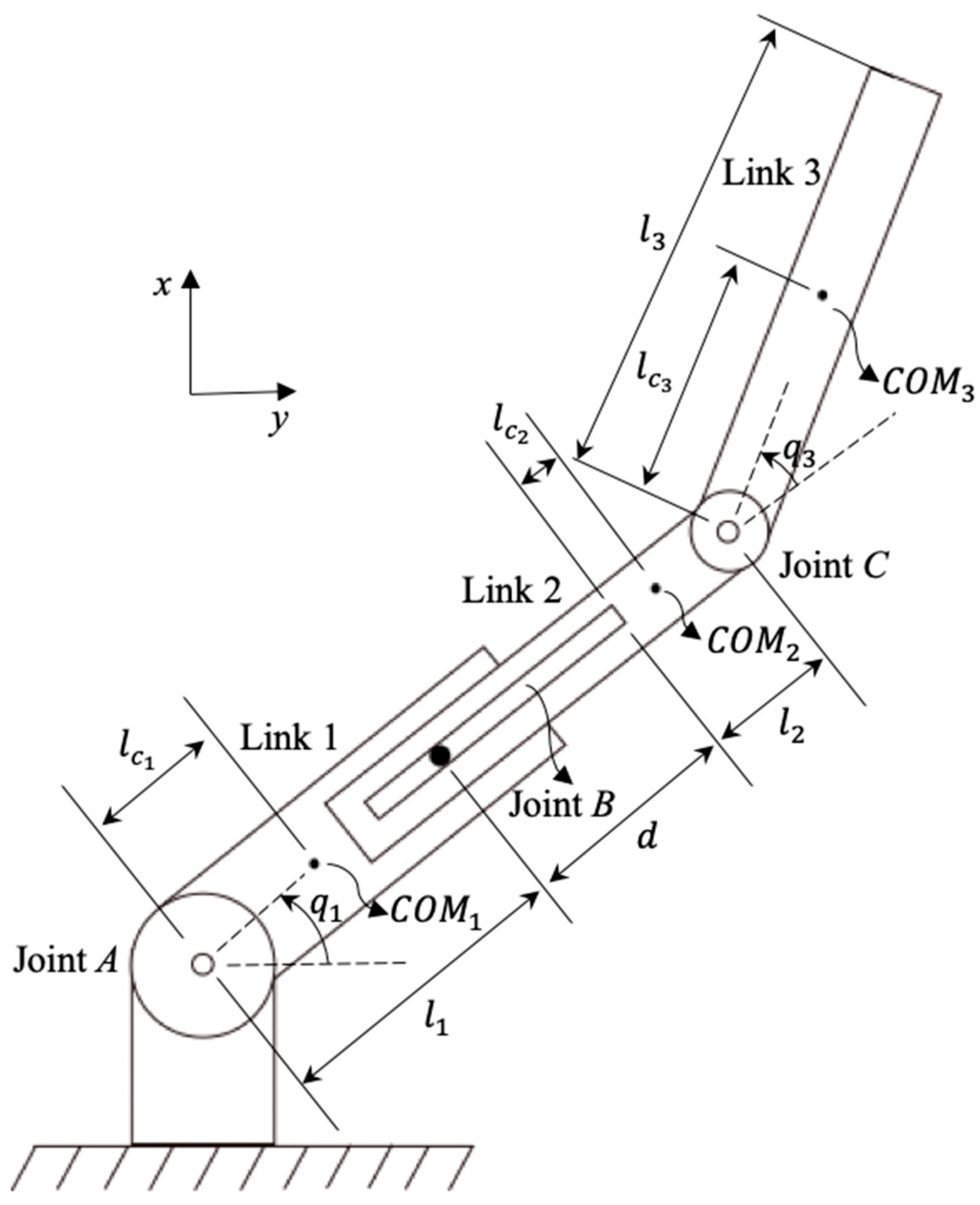
The dynamic modeling of the same three-link planar RPR robotic arm mechanism using the Euler–Lagrange equations of motion has previously been presented in a step-by-step manner [42]. As dynamic modeling is not the primary focus of this study, the resulting equations are provided directly rather than re-deriving them in full. The Euler–Lagrange equations of motion for the designed three-link planar RPR robotic arm mechanism are given in the following.

For Joint A:

$${\displaystyle \frac{d}{dt}}\left({\displaystyle \frac{\partial L}{\partial {\dot{q}}_1}}\right)-{\displaystyle \frac{\partial L}{\partial q_1}}={\tau }_1$$

(1)

where L represents the Lagrange function, ${\tau }_1$ refers to the joint torque at Joint A, $q_1$ denotes the angle of Joint A relative to the horizontal x-axis, and t refers to the time. By substituting all relevant terms, the following equation can be obtained:

$$\begin{gathered} \left(I{c}_1+m_{1}l{c}_1^2+I{c}_2+m_2{\left(l_1+d+l{c}_2\right)}^2+I{c}_3+m_{3}l{c}_3^2\right){\ddot{q}}_1+2m_2\left(l_1+d+l{c}_2\right){\dot{q}}_1\dot{d}+\left(I{c}_3+m_{3}l{c}_3^2\right){\ddot{q}}_3 \\ +m_{1}gl{c}_1\mathit{cos}{q}_1+m_{2}g\left(l_1+d+l{c}_2\right)\mathit{cos}{q}_1+m_{3}g\left(l_1+d+l_2\right)\mathit{cos}{q}_1 \\ +m_{3}gl{c}_2\mathit{cos}\left(q_1+q_3\right)={\tau }_1 \end{gathered}$$

(2)

where $l_1$ and $l_2$ represent the lengths of Link 1 and Link 2, respectively; $m_1,m_2$ and $m_3$ denote the masses of Links 1, 2 and 3, respectively; $l{c}_1, l{c}_2$ and $l{c}_3$ indicate the distances from the preceding joint to the center of mass of Links 1, 2 and 3, respectively; the moments of inertia about centers of mass for Links 1, 2 and 3 are denoted by ${Ic}_1, {Ic}_2$ and ${Ic}_3$, respectively; $q_1$ refers to the angle of Joint A relative to the horizontal x-axis; $q_3$ represents the angle of Joint C relative to Link 2; d corresponds to the extension of the prismatic Joint B; ${\dot{q}}_1$ and $\dot{d}$ denote the angular velocity of Joint A and the linear velocity of Joint B, respectively, while the terms ${\ddot{q}}_1$ and ${\ddot{q}}_3$ represent angular accelerations of Joint A and Joint C, respectively; and, finally, the term $g$ represents the acceleration due to gravity.

For Joint B:

$${\displaystyle \frac{d}{dt}}\left({\displaystyle \frac{\partial L}{\partial \dot{d}}}\right)-{\displaystyle \frac{\partial L}{\partial d}}=f$$

(3)

where $f$ denotes the external force applied at Joint B. Substituting all relevant terms into Equation (3), the following equation can be obtained:

$$\left(m_2+m_3\right)\ddot{d}-m_2\left(l_1+d+l_2\right){{\dot{q}}_1}^2+\left(m_2+m_3\right)g\sin q_1=f$$

(4)

where the term $\ddot{d}$ represents the acceleration of Joint B.

For Joint C:

$${\displaystyle \frac{d}{dt}}\left({\displaystyle \frac{\partial L}{\partial {\dot{q}}_3}}\right)-{\displaystyle \frac{\partial L}{\partial q_3}}={\tau }_3$$

(5)

where ${\tau }_3$ denotes the joint torque at Joint C. Substituting all relevant terms into Equation (5), the resulting equation can be expressed as follows:

$$\left(I{c}_3+m_{3}l{c}_3^2\right)\left({\ddot{q}}_1+{\ddot{q}}_3\right)+m_{3}g\mathit{cos}\left(q_1+q_3\right)l{c}_3={\tau }_3$$

(6)

Equations (2), (4) and (6) represent the Euler–Lagrange equations of motion of the designed three-link planar RPR robotic arm mechanism.

4. Application of Various Neural Network Algorithms for Regression Analysis

In the regression learner artificial neural network architecture, the angular acceleration of Joint A (${\ddot{q}}_1$) is assigned as the response variable, while the link masses are designated as predictors. All other variables, namely, the lengths of the links, torques at Joints A and C, and the force at Joint B, are held constant. The lengths of all three links are assumed to be equal, each measuring 1 m. The initial angle of Joint A ($q_1$) is set to 45°, the initial extension of Joint B (d) is 0.5 m and the initial angle of Joint C ($q_3$) is 30°. Gravitational acceleration ($g$) is taken as 9.81 m/s². The model starts with Joint A at 0.1 rad/s (${\dot{q}}_1)$, Joint B at 0.05 m/s ($\dot{d})$ and Joint C at −0.1 rad/s ${(\dot{q}}_3)$. The initial torques are set to 1 Nm for Joint A (${\tau }_1$) and −0.2 Nm for Joint C (${\tau }_3$), while the applied force at Joint B (f) is assumed to be 0.5 N. These initial values were selected randomly but are physically reasonable and appropriate for the designed robotic arm mechanism.

A total of 204 datasets were recorded, 10% of which were dedicated for testing purposes. Due to the large number of plots and similar results across outputs, only the regression models predicting the angular acceleration of Joint A (${\ddot{q}}_1$) are presented in this study. The analysis was conducted using the MATLAB R2024b Regression Learner App. The research analyzed six artificial neural network models, including narrow, medium, wide, bilayered, trilayered and optimizable neural networks. These models are pre-configured within the MATLAB Regression Learner App, and were selected for investigation based on their availability and applicability within the software environment.

5. Results

In this study, the link masses ($m_1, m_2$ and $m_3)$ were assigned as predictor variables, while the angular acceleration of Joint A (${\ddot{q}}_1$) was designated as the response variable. All neural network models investigated were based on the default configurations provided within the MATLAB Regression Learner App, with their parameters summarized in Table 2. In particular, the optimizable neural network was trained using Bayesian optimization. Three activation functions were defined for optimization: Sigmoid, hyperbolic tangent (tanh) and rectified linear unit (ReLU). The number of neurons in the first, second and third layers was set in the range between 1 and 300. The regularization strength (lambda) was allowed to vary within the range of 5.4348 × ${10}^{-8}$ to 543.4783. All of these parameter ranges were based on MATLAB’s default settings.

Table 1. Training results for the artificial neural network algorithms.

	Narrow Neural Network	Medium Neural Network	Wide Neural Network	Bilayered Neural Network	Trilayered Neural Network	Optimizable Neural Network
RMSE (Validation)	0.79793	0.58790	0.73327	0.80452	0.86791	0.34377
R-Squared (Validation)	0.92	0.96	0.94	0.92	0.91	0.99
MSE (Validation)	0.63670	0.34563	0.53769	0.64726	0.75326	0.11818
MAE (Validation	0.36581	0.23569	0.28751	0.34829	0.36830	0.066492
MAPE (Validation)	8.2%	5.7%	6.7%	7.9%	9.0%	1.6%
Prediction Speed (obs/s)	~25,000	~34,000	~13,000	~28,000	~41,000	~48,000
Training Time (s)	3.2583	2.5518	2.8335	3.562	1.7049	49.11
Model Size (kB)	~5	~6	~9	~7	~9	~22

presents the training results of the various artificial neural network models used for regression analysis. The optimizable neural network produced the lowest Root Mean Squared Error (RMSE) value, indicating it as the most accurate model among all tested models. In contrast, the trilayered, bilayered, wide, and medium models exhibited similar RMSE (validation) values, though slightly higher than that of the optimizable model. Furthermore, Table 1 shows that the R-squared (validation) value for the optimizable neural network was nearly 1.0, representing a near-perfect regression fit. While the R-squared values of the other models ranged between 0.9 and 1.0, the optimizable model demonstrated the value closest to 1.0, reinforcing its superior performance. The optimizable neural network produced the most effective results through its lowest Mean Squared Error (MSE), Mean Absolute Error (MAE) and Mean Absolute Percentage Error (MAPE) values. Despite its superior accuracy and fastest prediction speed among all the models, it required the longest training time. Table 1 also reveals that the optimizable neural network had the largest model size. On the other hand, the trilayered neural network exhibited the shortest training time, which is considered as a factor contributing to its comparatively poor performance regarding RMSE, R-squared, MSE, MAE and MAPE. However, it achieved the second-fastest prediction speed after the optimizable model.

Table 2. Model hyperparameters for the artificial neural network algorithms.

	Narrow Neural Network	Medium Neural Network	Wide Neural Network	Bilayered Neural Network	Trilayered Neural Network	Optimizable Neural Network
Number of Fully Connected Layers	1	1	1	2	3	3
First Layer Size	10	25	100	10	10	36
Activation	ReLU	ReLU	ReLU	ReLU	ReLU	Tanh
Iteration Limit	1000	1000	1000	1000	1000	1000
Regularization Strength (Lambda)	0	0	0	0	0	0.00012159
Second Layer Size	X	X	X	10	10	11
Third Layer Size	X	X	X	X	10	105

summarizes the characteristics of the investigated neural network models, which are the default parameter values in MATLAB. As seen in Table 2, the ReLU activation function was used in the narrow, medium, wide, bilayered and trilayered neural network models, while the hyperbolic tangent function (Tanh) was used in the optimizable neural network. According to Table 2, the optimizable neural network had greater second and third layer sizes than the bilayered and trilayered neural network models, while the wide neural network model had the largest first layer size. Due to their neural network architectures, the narrow, medium and wide neural networks models each included only one fully connected layer. According to Table 2, the regularization strength (lambda) was 0 for the narrow, medium, wide, bilayered and trilayered networks and 0.00012159 for the optimizable neural network. The strength of regularization grows with an increase in the lambda value. Additionally, the results indicated that the iteration limit was 1000 for all of the models.

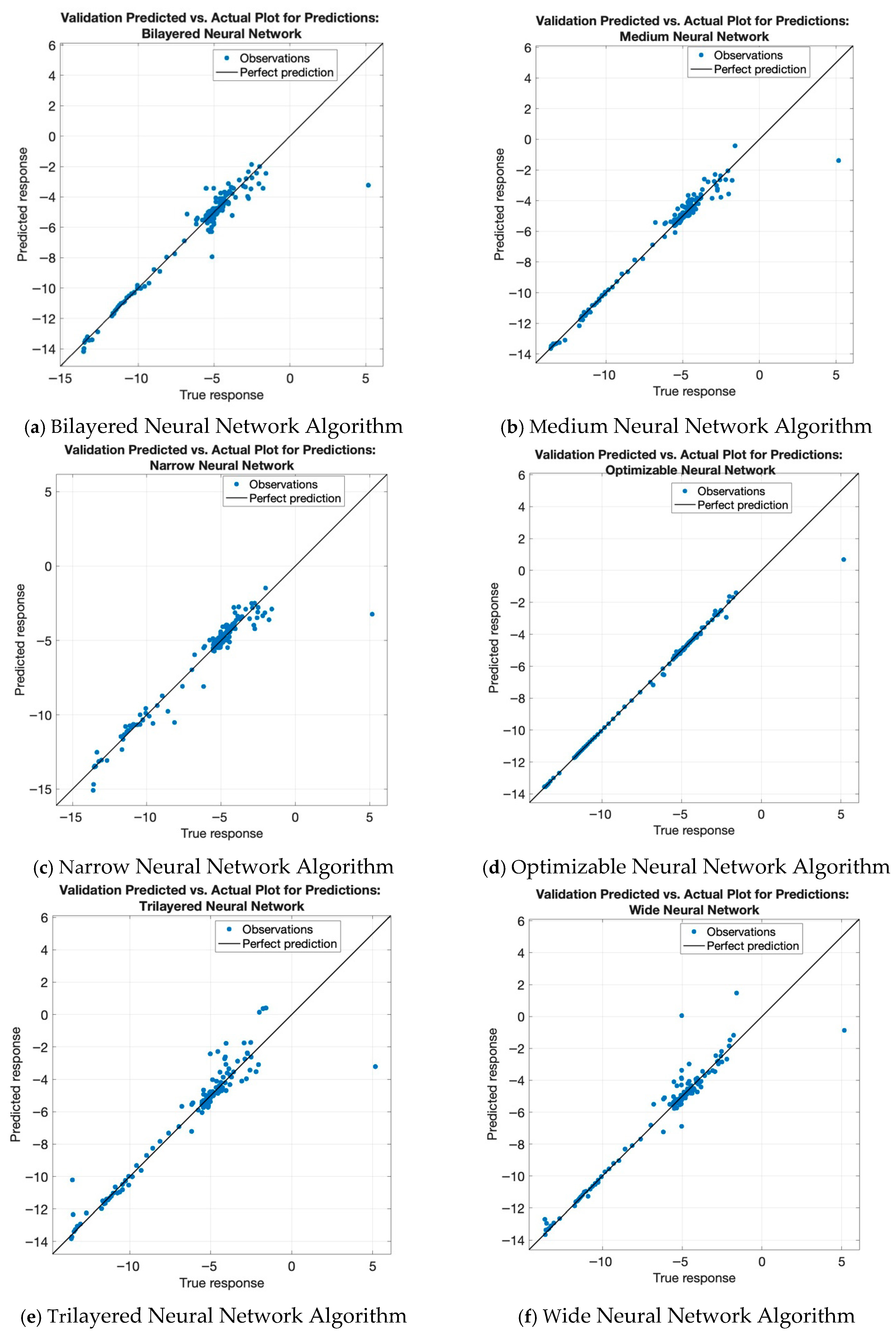
Figure 2 illustrates the predicted versus actual values for all neural network regression models investigated in this study. As shown in Figure 2a, the optimizable neural network demonstrated the best predictive performance, with nearly all observed data points closely aligned along the perfect prediction line. This result is consistent with the R-squared value reported in Table 1, which was nearly 1.0 for the optimizable model, indicating a near-perfect fit. The trilayered neural network produced the worst results, according to Figure 2e, as most observed points strongly differed from the perfect prediction line. Figure 2b illustrates that the medium neural network provided the second-best predictive performance, with the majority of observed values clustered around the ideal prediction line. The observed points in Figure 2a,c,f maintain similar patterns, staying near the perfect prediction line but not forming as tight a cluster as those observed for the optimizable and medium models.

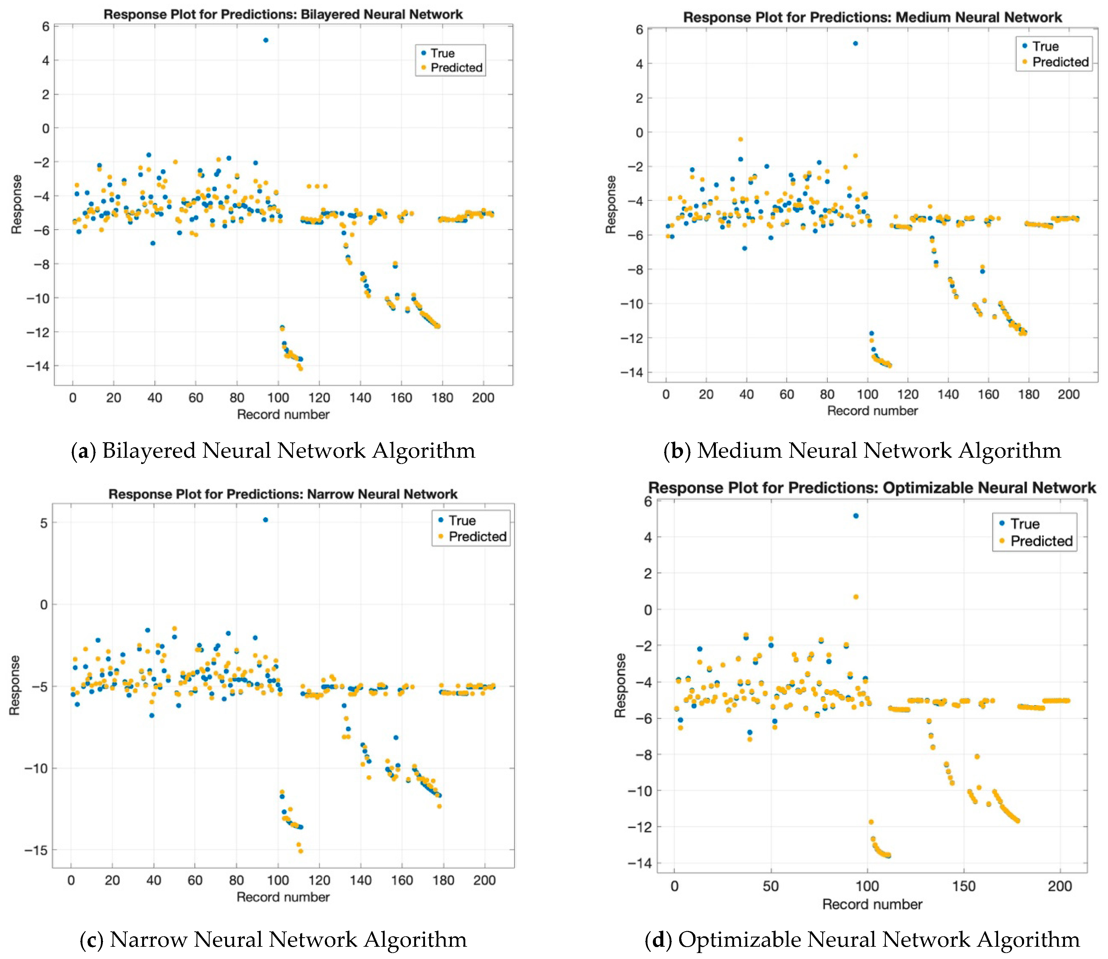
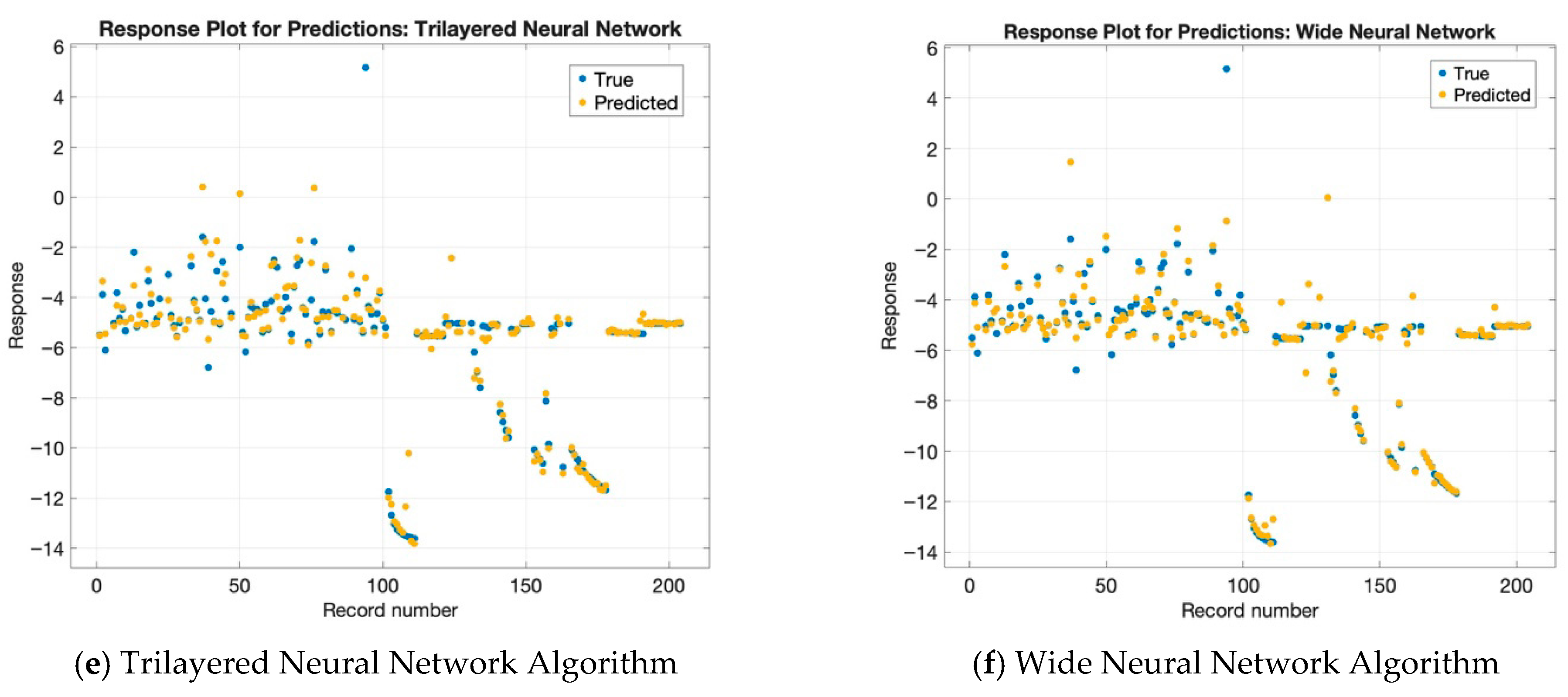
Figure 3 presents the response plots for each neural network model used in the prediction task. As shown in Figure 3d, the optimizable neural network model exhibited the best performance, with most of the predicted values closely matching the true values. In other words, this model produced the most accurate response plot among all those examined. In contrast, Figure 3a–c,e,f—corresponding to the bilayered, medium, narrow, trilayered and wide neural network models, respectively—do not display significant differences from one another. The models show a common pattern, where their most accurate predictions of actual values happen after reaching record number 120. Before this point, the models other than the optimizable neural network tended to show reduced prediction accuracy, indicating that the other models struggled to align their predicted values with actual observations in the earlier portion of the dataset.

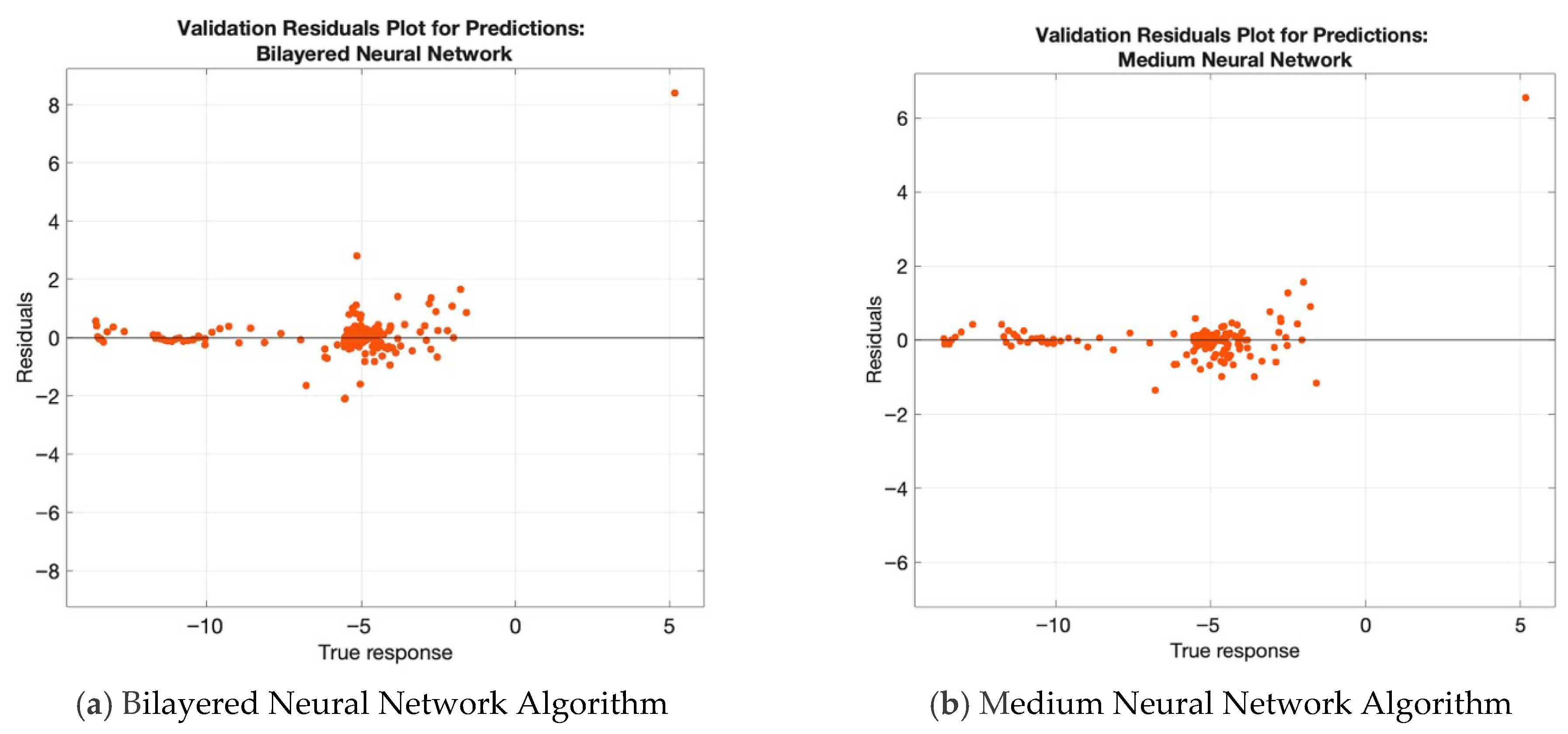
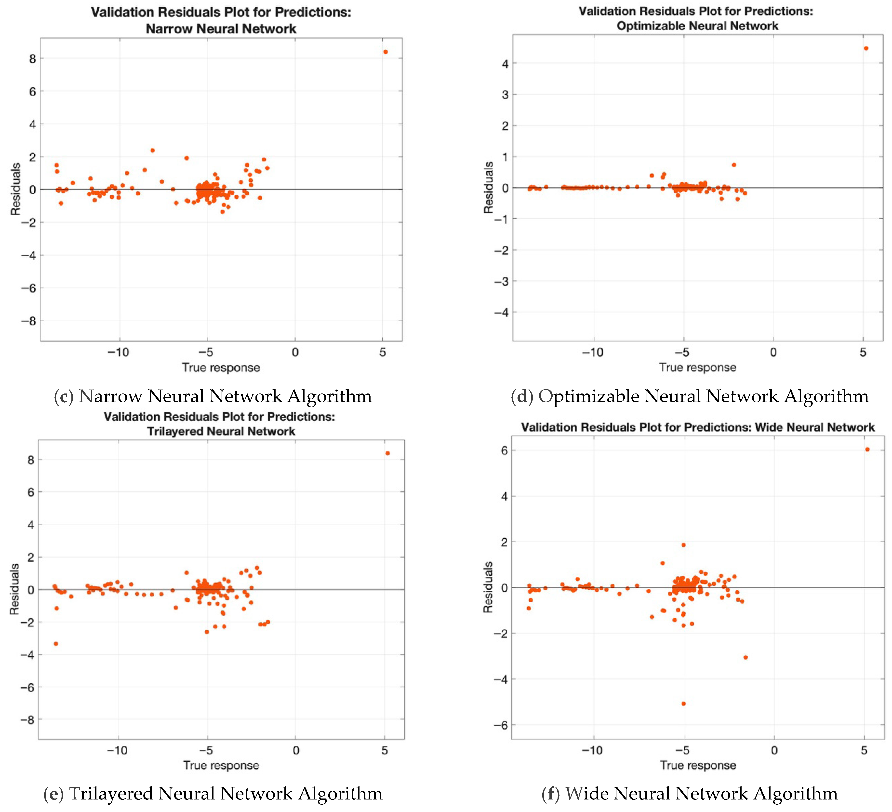
Figure 4 presents the residual plots for the predictions generated using each neural network algorithm investigated in this study. The residual plots display the degree of matching between the model predictions and the actual data points. The optimizable neural network showed the most accurate results, as can be seen from Figure 4d, as its residuals remained close to the zero line. In contrast, the predictions of the other neural network models exhibited larger residuals and less alignment with the actual data, as can be seen from Figure 4a–c,e,f. Furthermore, Figure 4 reveals that while the residual patterns across different models are similar, they remain independent of one another.

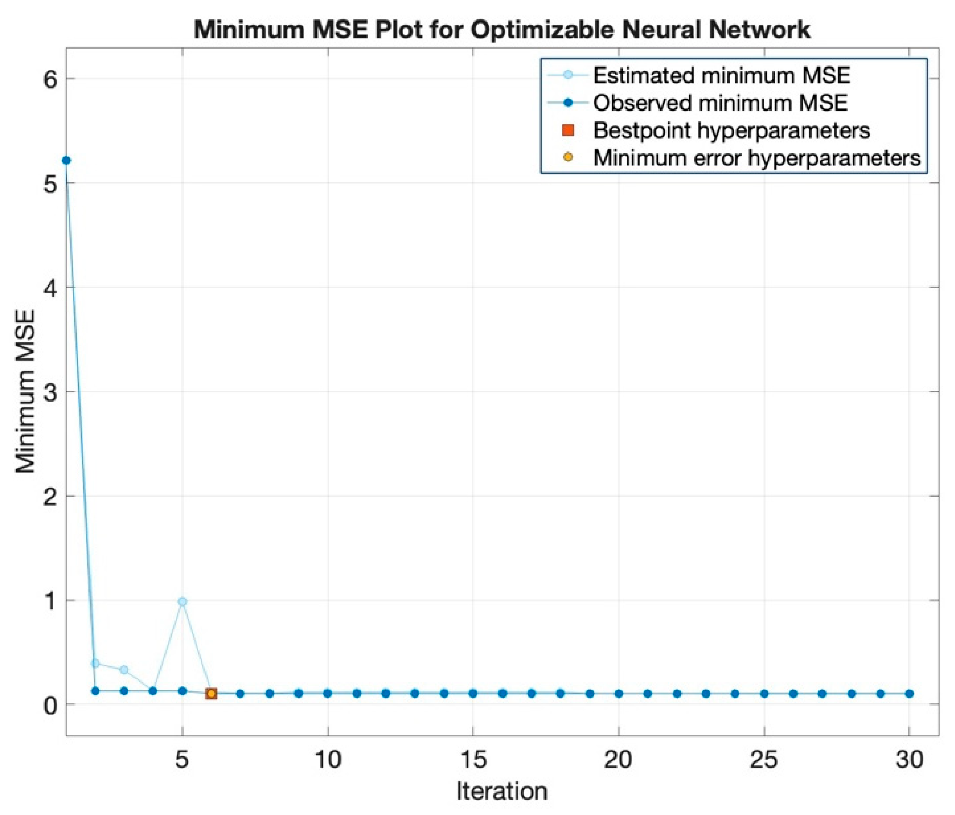
The minimum Mean Squared Error (MSE) plot for the optimizable neural network is shown in Figure 5, from which it can be seen that the total number of iterations reached 30. The optimal hyperparameters became apparent during the sixth iteration, as the minimum observed MSE reached 0.10382 and the regularization strength (lambda) was 0.00012159. Therefore, at this iteration, the estimated minimum MSE, observed minimum MSE, best hyperparameter values and minimum error hyperparameters were all additionally recorded.

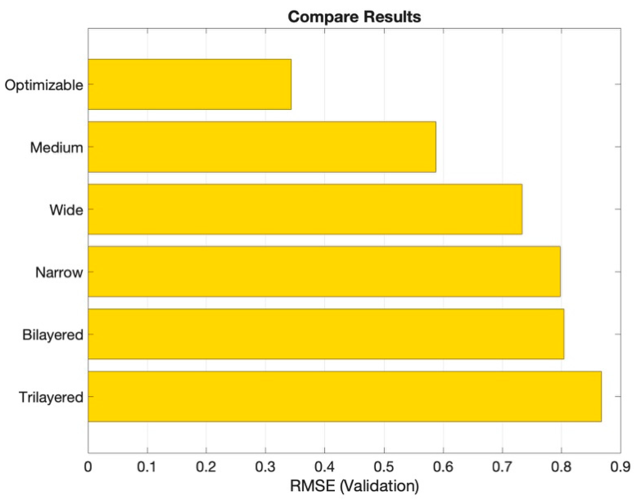
Figure 6 presents a comparison of the Root Mean Squared Error (RMSE) values for each artificial neural network regression model investigated in this study, from which it can be seen that the optimizable neural network regression model exhibited the lowest RMSE value, while the trilayered neural network model obtained the highest value. Specifically, the RMSE (validation) values were 0.8679, 0.8045, 0.7979, 0.7333, 0.5879 and 0.3438 for the trilayered, bilayered, narrow, wide, medium and optimizable neural network models, respectively.

6. Discussion

In this study, datasets were generated by varying the masses of the links, where the masses were initially restricted to the range between 0 and 1 kg. The regression results indicated that when the mass differences between the links were small, the regression models did not achieve optimal performance; furthermore, they showed no improvement when the mass differences exceeded 1 kg. Therefore, for accurate regression results, the links should not have mass differences exceeding 1 kg.

Although this study primarily presents regression models for the angular acceleration of Joint A, the same models were also applied to Joints B and C. The results for these joints were found to be very similar to those of Joint A; therefore, they were not included in this report.

The analysis indicated that the regression models would benefit from additional variables, which researchers could modify to achieve better results. In the present work, only the masses of the links were changed, while the link lengths, torques of Joints A and C, and force of Joint B were held constant. Future studies could analyze how different link lengths and masses collectively affect joint accelerations and regression performance, while also examining the effects of changing joint torques and forces.

Additionally, as the data in this study were collected under constant joint torques and forces, regression analysis could also be performed under natural oscillations resulting from gravity and inertia. Engineers can use neural networks to create innovative design solutions through the analysis of acceleration regression models under different operational conditions.

This study serves as a primarily investigation of a regression-analysis-based approach for the dynamic modeling of a robotic arm mechanism. The findings have the potential to inform future research, including the exploration of various mechanism configurations, joint angle variations or alternative dynamic modeling approaches.

7. Conclusions

In this study, various neural network regression models were applied for the dynamic modeling of a three-link planar RPR robotic arm mechanism. The Euler–Lagrange equations of motion were initially presented. Subsequently, narrow, medium, wide, bilayered, trilayered and optimizable neural network algorithms were employed for regression analysis based on these equations. The masses of the links were assigned as predictors, while the angular acceleration of Joint A was designated as the response variable; in other words, the acceleration of Joint A’s angle was predicted as a function of the link masses. The results indicated that the optimizable neural network algorithm outperformed the others and, therefore, can be recommended as the preferred regression model for dynamic modeling of the considered mechanism. Although the other neural network models generated comparable results, they did not show any particular performance advantages. This research revealed how link mass changes affect joint acceleration under constant joint torques and forces, as well as the performance of various neural network models in regression learning for robotic dynamic modeling, through an experimental approach which enables researchers to select suitable algorithms for specific applications. Future research should involve the application of diverse datasets, investigation of the effects of varying model parameters, and exploration of different robotic arm mechanism dynamic modeling using artificial neural networks.