Article

Data–Model Integration-Driven Temperature Rise Prediction Method for New Energy Electric Drive Bearings

1
School of Mechatronics Engineering, Henan University of Science and Technology, Luoyang 471003, China
2
Collaborative Innovation Center of Hennan Province for High-End Bearing, Henan University of Science and Technology, Luoyang 471000, China
*
Author to whom correspondence should be addressed.
Machines 2025, 13(10), 925; https://doi.org/10.3390/machines13100925
Submission received: 4 September 2025 / Revised: 4 October 2025 / Accepted: 5 October 2025 / Published: 7 October 2025

Abstract

Accurate prediction of bearing temperature rise offers essential support for equipment operation and optimized design. However, traditional methods often lack accuracy under the complex operating conditions of new energy electric drive bearings. To address this, we propose a model–data integration-driven approach for predicting the temperature rise in new energy electric drive bearings. First, a data-driven optimization method is employed to integrate mathematical and simulation models, generating highly reliable simulation data. Then, the simulation data and measured data are fused to construct an integrated dataset for bearing temperature rise. Finally, a CNN-LSTM prediction model is established and trained using this dataset. Validation experiments were carried out on the EV6206E-2RZTN/C3 bearing to verify the effectiveness of the proposed method. Results show (1) under constant operating conditions, the MAE during the temperature rise phase is 0.773 °C, and the steady-state phase maximum MAE is 0.686 °C, and (2) under variable operating conditions, the maximum MAE during the temperature rise phase is 0.713 °C, and the steady-state phase maximum MAE is 0.764 °C. The proposed method achieves effective prediction of temperature rise in electric drive bearings and offers a valuable reference for addressing temperature prediction challenges under complex operational conditions.

1. Introduction

Heat accumulation during bearing operation leads to a rise in temperature, and excessively high temperatures can impair bearing operational accuracy, service life, and even trigger equipment failures [1,2]. Accurate prediction of bearing temperature rise can help identify potential faults in advance, thereby ensuring operational safety. New energy electric drive bearings often operate under extremely complex conditions such as high speeds, variable loads, frequent starts and stops, and rapid acceleration or deceleration, making them more susceptible to failures caused by uncontrolled temperature rise. Therefore, developing an accurate prediction method for the temperature rise in new energy electric drive bearings not only provides safety assurance for the operation management of new energy vehicles and bearing performance tests, but also offers data support for the optimized design of such bearings.
Traditional methods for predicting bearing temperature rise primarily rely on analyzing the mechanisms of frictional heat generation and heat transfer within bearings. By studying the principles of temperature rise, mathematical models or finite element simulation models are established to forecast bearing temperature increase. Classical mathematical models for frictional heat generation include the empirical formula proposed by Palmgren [3] and the calculation model introduced by SKF [4]. However, mathematical modeling approaches are only suitable for scenarios where bearing operating conditions are relatively stable. Their prediction accuracy is insufficient for complex conditions such as high speeds and variable loads. Finite element methods, which involve building simulation models of temperature fields, can more accurately predict bearing temperature rise under complex operating conditions. Reference [5] investigated the temperature distribution of double-row tapered roller bearings for railways under test conditions using finite element analysis. Reference [6] analyzed the evolution of mechanical and thermal characteristics throughout the entire lifecycle of bearings under high ambient temperatures. Compared with mathematical modeling, finite element simulation delivers higher accuracy and a broader range of applicability. However, it involves capturing complex bearing kinematics and transient heat transfer processes. The significant computational demands often lead to simulation durations ranging from several hours to days. Moreover, these intricate calculations are frequently associated with convergence difficulties [7,8,9,10].
Adopting a method that integrates mathematical and simulation models, key parameters during the target system process are first calculated using mathematical models, which are then imported into simulation models. This approach significantly reduces computational costs while maintaining prediction accuracy. Reference [11] established a bearing simulation model driven by data–model integration to rapidly generate bearing operation data, addressing the issue of insufficient sample size for remaining life prediction. References [12,13] introduced new bearing degradation assessment methods by incorporating data into mechanistic models. With the continuous advancement of deep learning models in predictive capabilities, researchers have begun applying these models to the field of bearings [14,15]. DNN [16], LSTM [17], FNN, RBFNN, and GRNN [18] have all been utilized for bearing fault diagnosis or temperature prediction, fully demonstrating the feasibility of artificial intelligence technology in the field of bearing temperature rise prediction. Combining deep learning algorithms with other methods can further enhance predictive performance. Reference [19] combined a BP with a PSO algorithm to propose a PSO-BP model for predicting temperature at specific measurement points of motorized spindles under designated working conditions. Reference [20] used a combination of experimental and simulation data to create a training dataset and proposed a model integrating CNN and the Informer model for dynamically predicting the bearing temperature rise process. Reference [21] integrated SKF’s frictional temperature model with a BP and GA to develop a prediction model for forecasting bearing temperature changes. Reference [22] established a GA-BP neural network model based on numerical results. This model can predict the effects of nine factors on the central oil film thickness and outer ring temperature of bearings. Reference [23] proposed a physics-guided LSTM network based on the changing trends of time-frequency domain feature indicators of bearings during the degradation process, for predicting the RUL of bearings. Deep learning models can bypass complex heat generation and transfer mechanisms, enabling rapid and efficient prediction of bearing temperature rise. However, accurately predicting bearing temperature rise using deep learning models requires addressing two key issues:
  • Selecting an appropriate deep learning model.
  • Obtaining high-quality datasets for model training. Existing research indicates that single deep learning models often struggle to maintain prediction accuracy under complex working conditions. Furthermore, there is a general lack of measured data on bearing temperature rise in practical studies, leading to insufficient accuracy of prediction models when confronted with new operating conditions.
To address the issues of insufficient accuracy in mathematical models, prolonged finite element simulation times, the requirement of high-quality datasets for deep learning algorithms while measured data are inadequate, and the inability of single deep learning models to maintain prediction accuracy under complex working conditions, this study proposes the following approaches:
  • To tackle the problems of low accuracy in mathematical models and long finite element simulation times: By combining the rapidity of mathematical calculation models with the accuracy of simulation models, a data-driven finite element simulation model is established. Measured data are introduced to correct model parameters, thereby obtaining a high-precision and rapid simulation model.
  • To resolve the issue of deep learning algorithms requiring high-quality datasets while measured data are insufficient: A data–model integrated simulation model is utilized to generate bearing temperature rise simulation data covering all working conditions. The simulation data and measured data are fused through methods such as data fusion to form a hybrid dataset for new energy electric drive bearing temperature rise. A dataset update interface is provided to continuously incorporate new measured and simulation data, thereby expanding the coverage of working conditions in the dataset.
  • To address the problem of single deep learning models often failing to maintain prediction accuracy under complex working conditions: A spatiotemporal feature fusion prediction model, CNN-LSTM, is developed by integrating CNN’s ability to extract spatial local features and LSTM’s expertise in processing time-series data. The hybrid dataset is used to train the model, and a model update mechanism is introduced. When the model’s prediction deviation is significant, the dataset is updated with new simulation or measured data to retrain the prediction model, ensuring its accuracy.

2. Methodology Framework

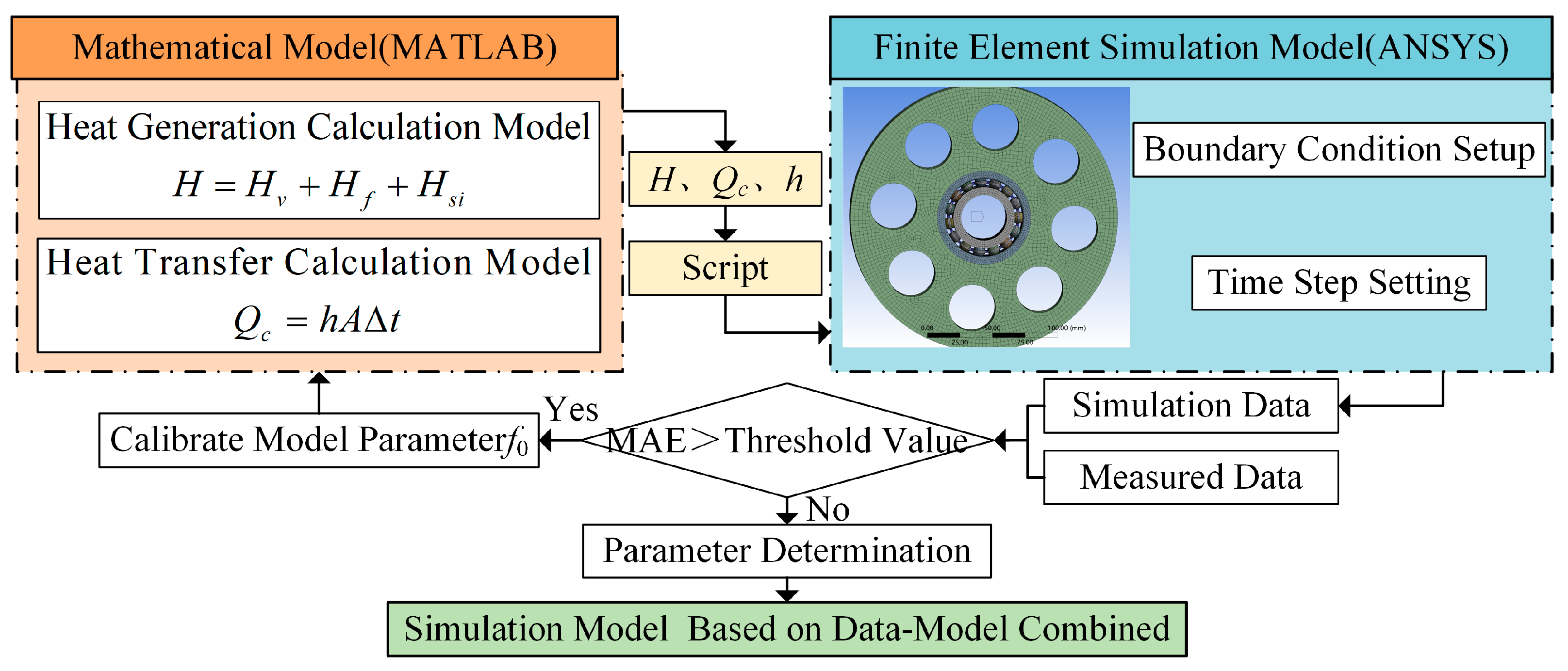
The overall architecture of the data–model integration-driven method for predicting temperature rise in new energy electric drive bearings is shown in Figure 1. The detailed operational mechanism of the method is as follows:
  • Establishment of a Data-Driven Simulation Model: Based on the mechanisms of bearing frictional heat generation and heat transfer, a bearing heat generation calculation model and a bearing heat transfer calculation model are established. The simulation conditions are determined according to the measured data conditions. First, the frictional heat generation quantity H is calculated using the bearing heat generation model. The heat exchange quantity Qc and surface heat transfer coefficient h are calculated using the bearing heat transfer calculation model. Then, H, Qc, and h are input into the finite element simulation model. Temperature rise simulation data under the specified working conditions are obtained through finite element simulation. The MAE between the simulation data and the measured data is compared. If the MAE exceeds a critical threshold, the parameter f0 (a coefficient related to bearing type and lubrication method) in the heat generation calculation model is optimized using the gradient descent method until the MAE falls below the critical value. This process determines the model parameters and yields a simulation model that meets the required accuracy standards.
  • Establishment of a Hybrid Dataset: The calibrated simulation model is utilized to generate temperature rise simulation data covering missing working conditions. This data can also guide supplementary bearing temperature rise tests to obtain corresponding measured data. Newly acquired measured data can, in turn, be used to further calibrate the simulation model, continuously enhancing its accuracy and adaptability to different working conditions, thereby improving the quality of data used for model training. Measured data and simulation data undergo normalization to eliminate dimensional differences. An interpolation method is employed to fill in missing values. Timestamps of measured and simulation data are aligned. A weight allocation strategy is applied to maximize the predictive value of the processed data, ultimately constructing a hybrid dataset comprising training, validation, and test sets. The dataset retains an update interface to continuously incorporate new measured and simulation data.
  • CNN-LSTM Prediction Model and Update Mechanism: A CNN-LSTM prediction model integrating spatiotemporal features is established by combining CNN’s capability for extracting local spatial features with LSTM’s expertise in processing time-series data. The model inputs include speed, load, time, and the temperature from the previous time step, while the outputs are time and temperature. The model parameters are trained using the training set from the hybrid dataset. The validation set is utilized for hyperparameter tuning to optimize model performance. The test set is employed to evaluate the prediction accuracy of the model, ultimately yielding a prediction model that meets the required precision standards. During model application, accuracy can be monitored by comparing predictions with measured data and simulation results. When the model accuracy falls outside the predefined acceptable range, the model can be retrained using an updated dataset to recalibrate its predictive performance.

3. Model Construction

The methodology for constructing a temperature rise simulation model for new energy electric drive bearings based on data–model integration is illustrated in Figure 2. The specific construction steps are as follows:
  • Mathematical Calculation Model: Based on the mechanisms of bearing frictional heat generation and heat transfer, parameterized heat generation and heat transfer calculation models are established in MATLAB2023(a). Input parameters include bearing geometric parameters, material properties, thermodynamic parameters, grease-air characteristics, and operational conditions. Physical quantities such as H (heat generation), Qc (heat exchange), and h (surface heat transfer coefficient) are computed. The results are saved in text format (TXT) for use by the finite element model.
  • Finite Element Simulation Model Setup: A full-scale model of the bearing is created in SOLIDWORKS, retaining key heat transfer features. Non-thermally sensitive structures such as fillets are removed to improve computational efficiency. Material properties are assigned to each part of the bearing, and the model is meshed with local refinement at contact areas to enhance simulation accuracy.
  • Transient Temperature Rise Simulation: Using an APDL script in ANSYS2023.R1, the heat generation data generated by MATLAB2023(a) is read, and the bearing heat generation load is imported into the heat transfer model. Thermal boundary conditions—including heat conduction, heat convection, and thermal loads—are applied sequentially. The initial temperature and ambient temperature are set, followed by time step configuration aligned with the measured data acquisition duration to ensure temporal alignment. Complete temperature rise simulation data (including time, speed, load, and temperature) are output and saved in CSV format.
  • Model Parameter Calibration: The MAE between measured and simulated data is calculated and defined as the objective function. A critical MAE threshold is set based on accuracy requirements. The parameter f 0 in the heat generation model is optimized using the gradient descent method until the MAE falls below the threshold. This process determines the final model parameters and completes the construction of the high-fidelity simulation model.

3.1. Mathematical Model

  • Frictional Heat Generation Model:
Based on the empirical formula proposed by Palmgren [1], the frictional heat generated during bearing operation is calculated. The main sources of bearing frictional heat include frictional power loss H v caused by grease viscosity, frictional power loss H f induced by load, frictional power loss H s i resulting from spinning and sliding of rolling elements. The total frictional power loss H of the bearing is given by
H = H v + H f + H s i
where the frictional power loss Hv caused by grease viscosity is given by
H v = 1 2 ω r o l l ( D d e + D d i ) M v
M v = 160 × 10 7 f 0 d m 3 , ( v n < 2000 ) 10 7 f 0 ( v n ) 2 / 3 d m 3 , ( v n 2000 )
where ω r o l l —angular velocity of rolling elements relative to the outer raceway ( rad / s );
D —bearing outer diameter ( mm );
d e —outer raceway groove bottom diameter ( mm );
d i —inner raceway groove bottom diameter ( mm );
M v —inner raceway groove bottom diameter ( mm );
f 0 —coefficient related to bearing type and lubrication method, ranging from 1.5 to 2;
d m —bearing pitch diameter ( mm );
v —kinematic viscosity of the grease at operating temperature ( mm 2 / s );
n —bearing speed ( r / min ).
2.
Heat Transfer Model:
The temperature field generated during bearing operation induces heat exchange within the bearing. Given the relatively small temperature difference within electric drive bearings, heat transfer primarily occurs through conduction and convection. Convective heat transfer can be calculated using Newton’s law of cooling:
Q c = h A Δ t
where Q c —heat transfer rate due to convection ( W );
h —heat transfer coefficient ( W / ( m 2 · K ) );
A —surface area involved in heat transfer ( m 2 );
Δ t —temperature difference between the bearing surface and the surrounding medium (K).
Methods for Calculating Surface Heat Transfer Coefficient h:
h = 0.332 k x P r 1 3 R e 1 2 , R e < 5 × 10 5 ( 0.37 R e 0.8 850 ) k x P r 1 3 , 5 × 10 5 R e < 10 7
where R e —Reynolds number, R e = u x / v ;
P r —Prandtl number for grease;
u —relative flow velocity of the grease with respect to the heat transfer surface ( m / s );
k —thermal conductivity of the grease ( W / ( m / K ) ).
3.
Model Parameter Optimization:
The coefficient to be determined in the model is f0 in Equation (3). Its initial value is set to 1.75. The parameter calibration problem is transformed into a constrained optimization problem by defining the objective function as the MAE between the measured and simulated data. Finally, the parameter is optimized and determined using the gradient descent method:
J ( f 0 ) = 1 N i = 1 N T s i m ( t i ; f 0 ) T r e a l ( t i )
min f 0 J ( f 0 ) ,   s . t .   1.5   f 0 2
where T s i m —simulated temperature from transient thermal analysis;
T r e a l —measured temperature;
N —total number of data points.

3.2. Finite Element Simulation Model

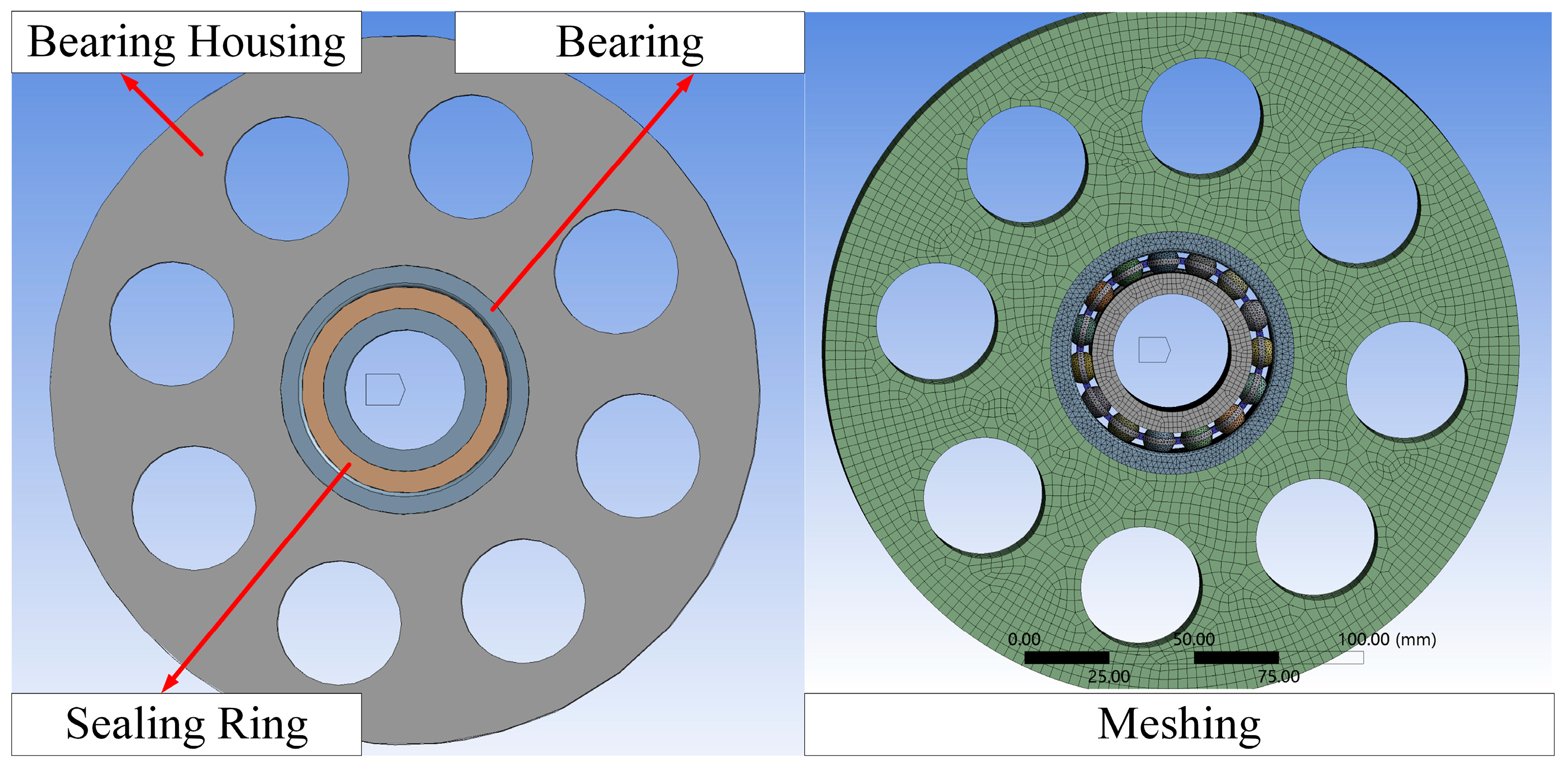
First, a full-scale model of the bearing is created in SOLIDWORKS based on its geometric dimensions, and the completed model is then imported into ANSYS2023.R1. To improve model accuracy, the model includes the inner ring, outer ring, cage, sealing ring, and bearing housing, with mesh refinement applied to contact areas. The model is shown in Figure 3. Next, boundary conditions and loads are applied to the model. The specific steps are as follows:
  • Set Thermal Conduction: After creating the model, appropriate material properties need to be assigned. After importing the material library, correct material properties such as density, specific heat capacity, and thermal conductivity are assigned to the geometry to ensure accurate characterization of the model’s thermal conduction behavior.
  • Define Thermal Convection: For thermal convection settings, select the appropriate mode in the “Convection” option, then choose the acting surface. Click “Details of Convection”, enter the corresponding value in the “Film Coefficient” under “Definition”, and input the ambient temperature in the “Ambient Temperature” field to complete the addition of thermal convection conditions.
  • Define Thermal Loads: Based on specific operational requirements, first calculate the heat generated by each part of the bearing. Then, apply these heat values as thermal loads to the corresponding locations such as the inner ring, outer ring, balls, and cage. This step ensures accurate simulation and application of thermal loads.
  • Set Time Steps: During transient analysis, appropriate time step parameters need to be defined. This includes the total simulation time, the number of time steps, and the time step size. These parameters determine the time range of the simulation and the resolution of the analysis.

4. Hybrid Dataset

To enhance dataset quality and improve the prediction performance of deep learning models, raw data undergo preprocessing and fusion. The specific steps are as follows:
  • Normalize both measured and simulated data to eliminate dimensional differences between them.
  • Apply interpolation to fill in missing values and ensure data completeness.
  • Align timestamps of measured and simulated data to guarantee strict synchronization of bearing temperature and environmental parameters on the time scale.
  • Maximize the predictive value of processed data through a weight allocation strategy. Since simulated data exhibit higher precision while measured data contain random disturbances, simulated data are assigned higher weights during fusion, whereas measured data are assigned lower weights.
  • Construct a hybrid dataset comprising training, validation, and test sets based on the weighted fused data.
  • The dataset retains an update interface to continuously incorporate new measured and simulated data.

5. Temperature Rise Prediction

5.1. CNN-LSTM Temperature Rise Prediction Model

The structure and data flow of the CNN-LSTM bearing temperature rise prediction model are illustrated in Figure 4. During model training, inputs include the current speed, load, timestamp, and the temperature from the previous time step. First, the CNN layer extracts combined features, interaction patterns, and local dependencies among these input features, achieving data dimensionality reduction and key information refinement. Then, the LSTM layer, with its unique gating mechanisms (input gate, forget gate, and output gate), captures long-term dependencies in the feature sequences output by the CNN along the time dimension. Through the synergistic effect of both components—CNN focusing on feature fusion and refinement, and LSTM specializing in temporal dynamic modeling—the model learns the complex nonlinear mapping relationship between the input parameters (speed, load, timestamp, and previous temperature) and the output (predicted temperature for the next time step), enabling accurate prediction of bearing temperature rise.

5.2. CNN

Compared with traditional feature extraction methods, using CNN allows for more effective extraction of relevant information from data. By sliding a convolutional kernel, local matrices are extracted and subsequently transformed to produce the output matrix of the convolutional layer. The convolution operation is defined as follows:
x l i = f ( x l 1 i × K l i + b l i )
where x l i —the i -th output feature map of the l -th convolutional layer;
x l - 1 i —the i -th input feature map from the l 1 -th layer;
K l i —the weight matrix of the i -th kernel in the convolutional layer l ;
b l i —the bias term.

5.3. LSTM

The forget gate is the most critical component in the LSTM, as it controls how much historical information to discard based on the characteristics of previous states, thereby mitigating issues such as gradient vanishing and explosion. The mathematical expression of the forget gate is as follows:
f t = σ ( W f [ h t 1 , x t ] + b f )
where xt—input at the current time step t , ht−1—hidden state at the previous time step t−1, and σ —Sigmoid activation function. The input gate controls how much new information is stored in the cell state. Its calculation formula is
i t = σ ( W i [ h t 1 , x t ] + b i )
C t = tanh ( W C [ h t 1 , x t ] + b C )
C t = f t C t + i t C t
where C t —candidate value for the cell state, C t —new cell state, and tanh: hyperbolic tangent activation function. The output gate controls the information output from the current cell state. Its specific calculation formula is
o t = σ ( W o [ h t 1 , x t ] + b o )
h t = o t tanh ( C t )
In Equations (8)–(14), W f , W i , W C , W o are weight matrices, b f , b i , b C , b o are bias terms, and h t is hidden state carrying information to the next time step.

5.4. Computational Process

(1)
CNN Computational Process: A CNN extracts local features by applying convolution kernels through sliding window operations over the input feature maps. For each output channel, the algorithm iterates over each spatial location of the output feature map. At each location, it computes the dot product between the local input region and the convolution kernel, adds a bias term, and generates the output feature map through an activation function.
(2)
LSTM Computational Process: The LSTM controls information flow through gating mechanisms, addressing the gradient vanishing problem in traditional RNNs. The forget gate determines how much previous memory to retain, the input gate controls the incorporation of new information, and the output gate regulates the output of the current hidden state. The cell state acts as a memory carrier, propagating information across time steps.

6. Validation and Application

Temperature rise prediction experiments were carried out on e-drive bearings for new energy vehicles. The feasibility of the proposed method was evaluated by comparing the MAE between the predicted results from different methods and the actual measured data.

6.1. Test Equipment

A dedicated performance test rig for new energy vehicle electric drive bearings was utilized to conduct temperature rise tests on the specialized bearing model SKF EV6206E-2RZTN/C3 (made in Shanghai, China). The objective was to obtain temperature rise data under typical operating conditions. The physical test rig and the layout of its temperature measurement points are shown in Figure 5. The parameter settings for the bearing variable-speed tests are summarized in Table 1.
The test system employs PT100 platinum resistance temperature sensors, with a speed range of 0–30,000 r / min , a radial loading range of 0–12 kN , and an axial loading range of 0–5 kN . Test conditions included: variable-speed conditions, rapid variable-speed conditions under high temperatures, gradually variable conditions, constant-load conditions and constant-speed conditions. Measured temperature rise data under all the above conditions were recorded and stored.

6.2. Method Validation

  • Simulation Model
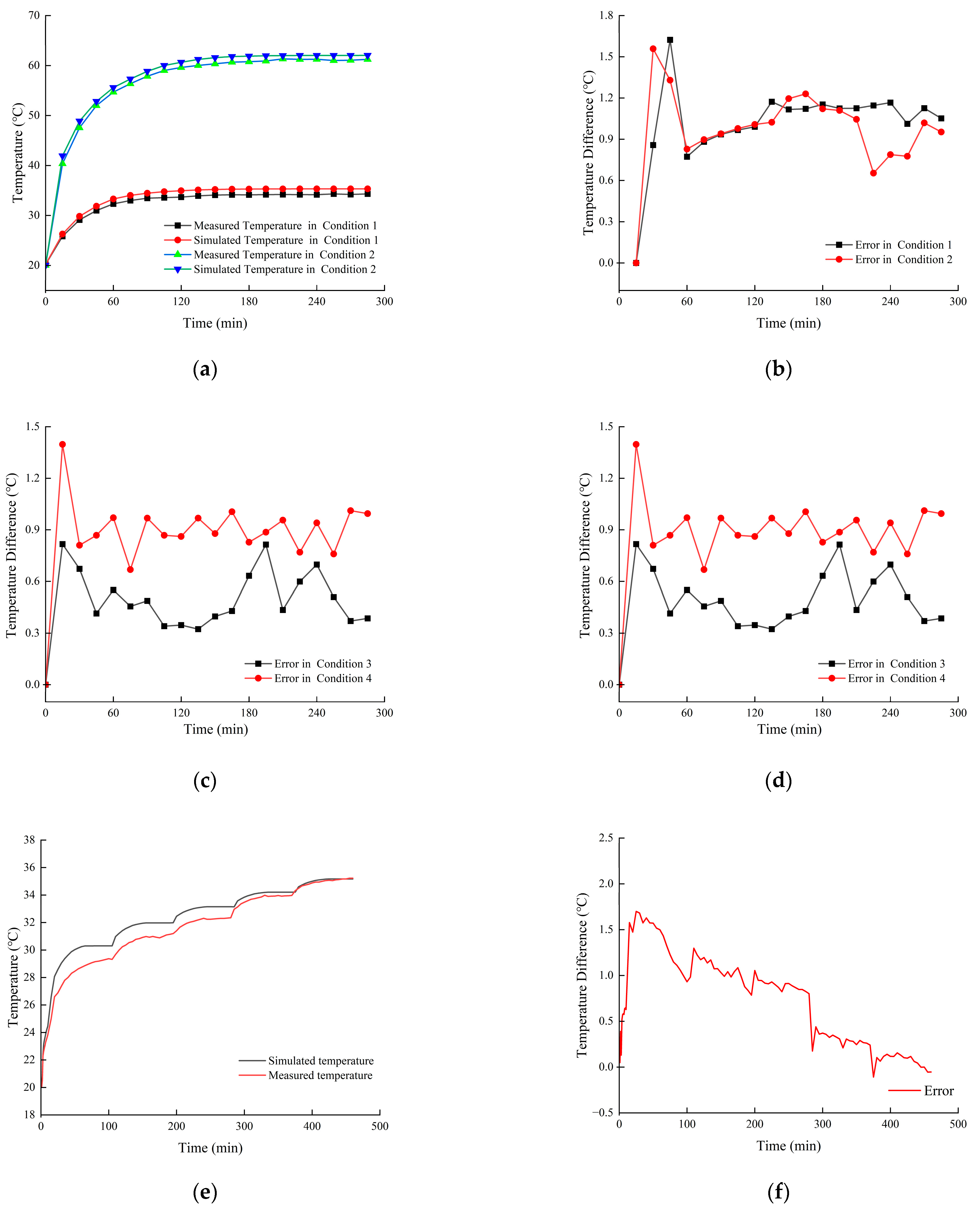
Based on the structural parameters of the test bearing, a data–model integrated simulation model was constructed using the method described in Section 3 of this paper. The maximum errors and MAE between the simulated and measured temperatures under different working conditions are shown in Table 2, and the comparison of the temperature rise process is illustrated in Figure 6. As shown in Table 2, the maximum temperature error under the five working conditions is less than 1.6 °C, and the MAE is less than 1.1 °C. As depicted in Figure 6, the simulated temperature rise trend aligns well with the measured data, with only minor errors between the simulated and experimental results.
2.
Hybrid Dataset
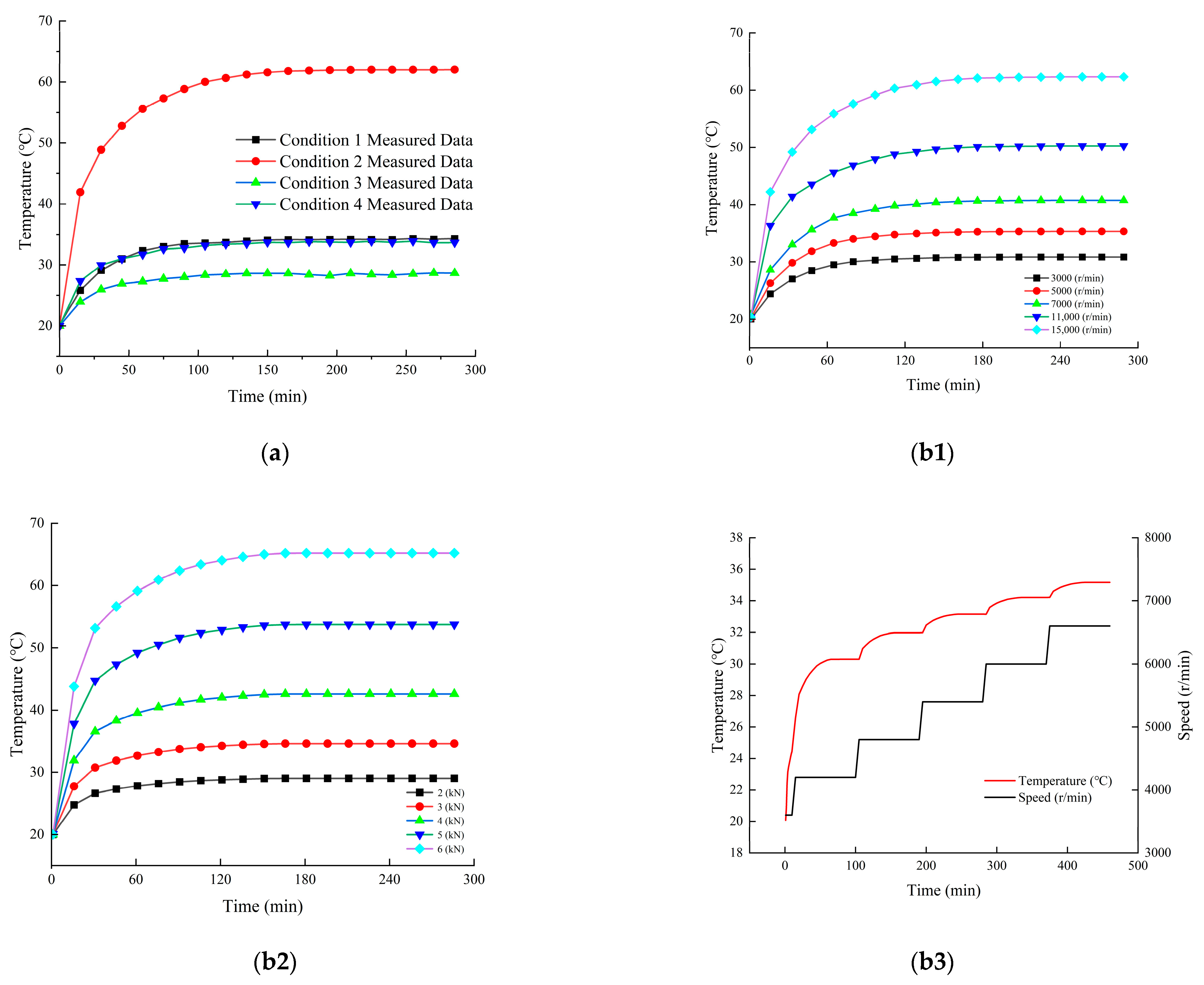
Simulation data and measured data were combined in a 7:3 weight ratio to form a hybrid dataset. This dataset was then divided into training, validation, and test sets in a 7:2:1 ratio. A subset of the dataset is illustrated in Figure 7. In Figure 7, Condition a, Condition 1: radial load 2 kN , speed 5000 r / min ; Condition 2: radial load 2 kN , speed 15,000 r / min ; Condition 3: radial load 2 kN , speed 3600 r / min ; Condition 4: radial load 3 kN , speed 3600 r / min . Condition b1: radial load 2 kN , speeds: 3000, 5000, 7000, 11,000, 15,000 r / min ; Condition b2: speed 3600 r / min , radial loads: 2, 3, 4, 5, 6 kN ; Condition b3: radial load 2 kN , speed range: 3600–6600 r / min .
3.
Validation of the CNN-LSTM Method
The parameters of the CNN-LSTM model were configured using the training and validation sets from the hybrid dataset. The specific parameters of the model after optimization and selection are summarized in Table 3.
Using the test set from the hybrid dataset, sequentially apply Algorithm 1 and Algorithm 2 to compute and obtain the prediction results of the CNN-LSTM model. Then, compare its predictive performance with that of the BP model and the LSTM model to evaluate the predictive performance of the proposed method in this paper.
Algorithm 1 Computation of convolutional layers
Input:
Input feature map: X ( H , W , C i n )
Convolutional kernel: W ( K h × K w × C i n × C o u t )
Bias: b ( C o u t )
Output:
Output feature map: X ( H , W , C o u t )
Steps:
1. Compute output size :   H = [ ( H K h ) / s ] + 1 , W = [ ( W K w ) / s ] + 1
2. Initialize output feature map X to zero.
3. for k = 0   to   C o u t 1     do   Traverse output channels
4.     for i = 0   to     H 1   do   Traverse output height
5.         for j = 0   to  W 1   do   Traverse output width
6.         X [ i , j , k ] m = 0 K h 1 n = 0 K w 1 c = 0 C i n 1 X [ i s + m , j s + n , c ] W [ m , n , c , k ] Compute feature map
7.         X [ i , j , k ] X [ i , j , k ] + b [ k ] Add Bias
8.         X [ i , j , k ] Aactivation ( X [ i , j , k ] ) Apply activation function
9.         end for
10.     end for
11. end for
12. return X Return output feature map
End Algorithm
Algorithm 2 Computation of LSTM units
Input:
Current time step input vector: x t
Previous   hidden   state :   h t 1
Previous   cell   state :   c t 1
Weight   matrix :   W f , W i , W c , W o
Bias vector: b f , b i , b c , b o
Output:
Current   hidden   state :   h t
Current   cell   state :   c t
1 .   Concatenate   inputs :   z concatenate [ h t 1 ; x t ] Vector concatenation
2 .   Compute   forget   gate :   f t σ ( W f z + b f ) σ is the sigmoid function
3 .   Compute   input   gate :   i t σ ( W i z + b i )
4. Compute candidate cell state: c t tanh ( W c z + b c )
5. Update cell state: c t f t c t 1 + i t c t denotes element-wise multiplication
6 .   Compute   output   gate :   o t σ ( W o z + b o )
7. Compute hidden state: h t o t tanh ( c t )
8 .   return   h t , c t Return current hidden state and cell state
End algorithm
  • Comparison of Temperature Rise Prediction Results for Electric Drive Bearings under Constant Operating Conditions
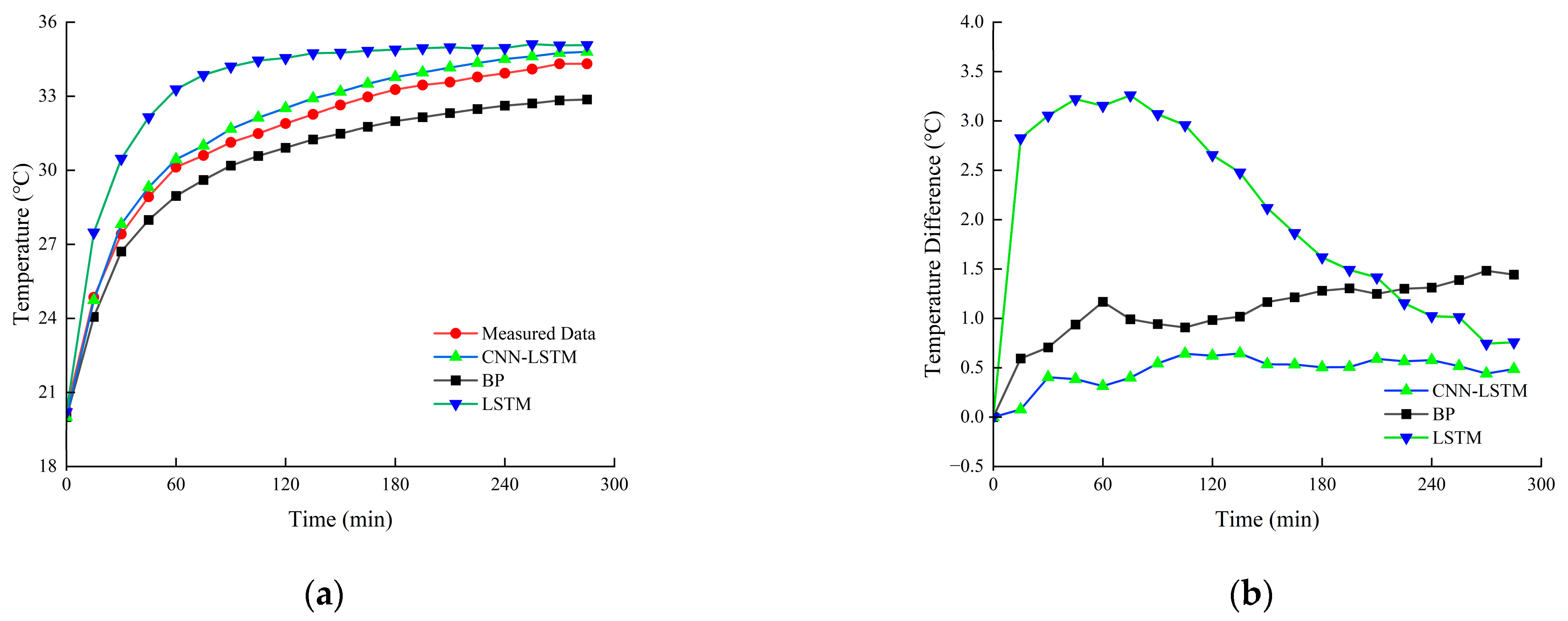
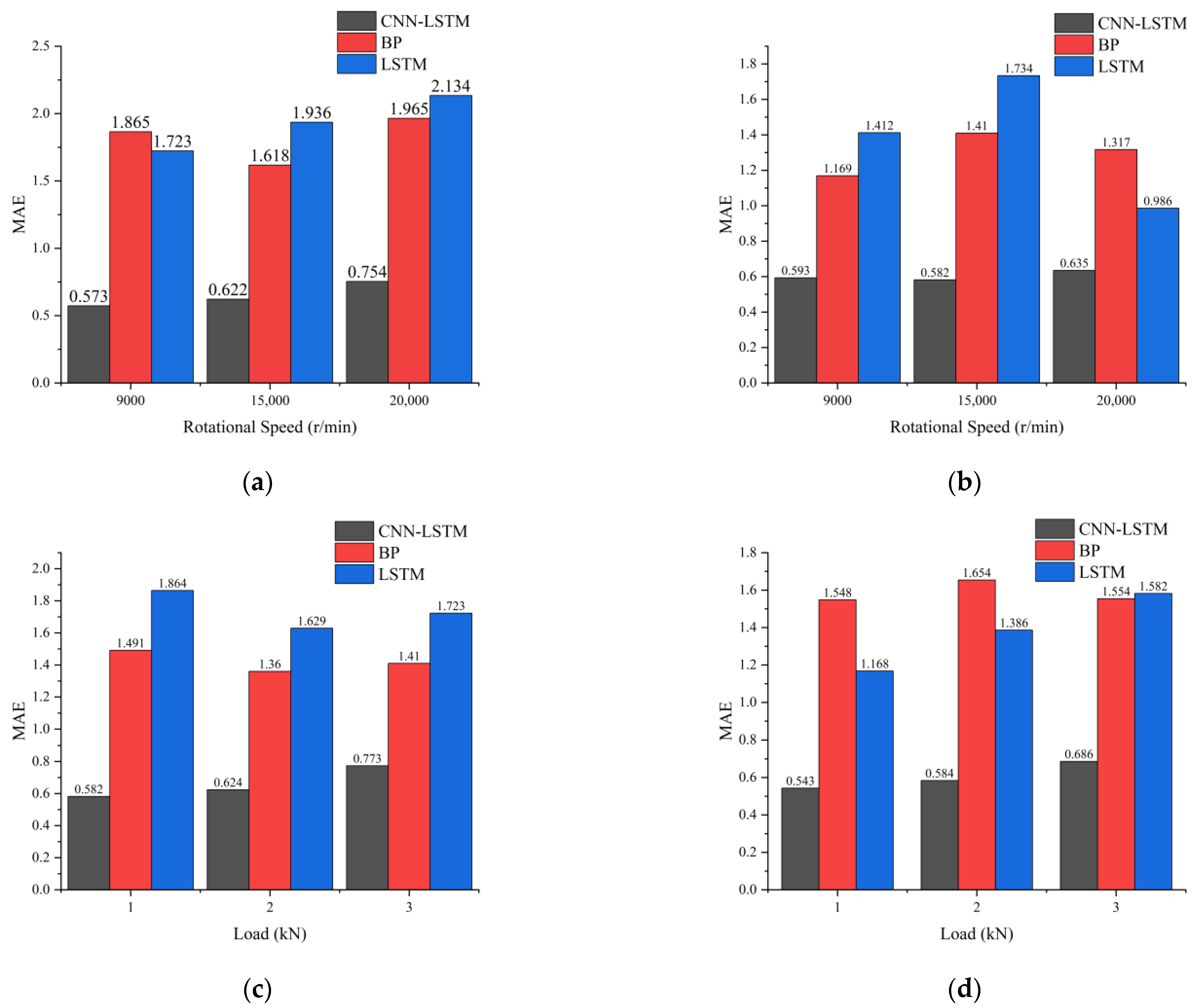
The temperature rise in the electric drive bearing under a load of 2 kN and a speed of 5000 r / min was predicted. The prediction results and errors of different models are shown in Figure 8. The prediction errors of the three models under different working conditions are shown in Figure 9. Throughout the entire temperature rise process, the following applied: During the temperature rise phase, both the CNN-LSTM and BP models maintained errors within 1 °C, demonstrating good prediction performance, while the maximum error of the LSTM model exceeded 2 °C. In the steady-state phase, the error of the LSTM model gradually decreased, the error of the BP model progressively increased, and the error of the CNN-LSTM model remained stable at around 0.5 °C. Overall, the CNN-LSTM prediction model achieved the smallest error with the most stable error fluctuation. The maximum error of the CNN-LSTM model during the temperature rise phase was 0.773 °C, and during the steady-state phase, it was 0.686 °C. Under all six working conditions, the error was maintained within 1 °C, indicating that the CNN-LSTM model exhibits excellent stability and accuracy in predicting bearing temperature rise under constant operating conditions.
2.
Comparison of Temperature Rise Prediction Results for Electric Drive Bearings under Variable Operating Conditions
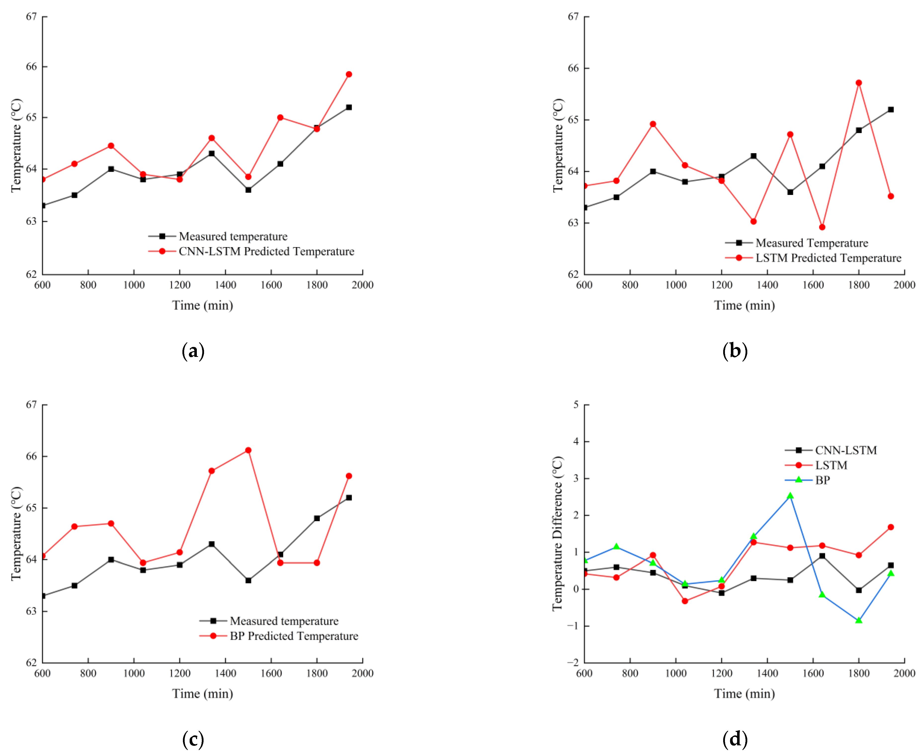
Figure 10 displays the prediction results of the three models for the temperature rise process of the electric drive bearing under these conditions. The experimental condition parameters are shown in Figure 11. In the initial stage, the predicted values and variation trends of all three models approximate the measured data, indicating that all models can capture the temperature change characteristics of the bearing during the steady-state phase under rapid variable-speed conditions. However, as time progresses, the predicted values of the BP and LSTM models gradually deviate from the measured values, and their errors increase. In contrast, the error of the CNN-LSTM model remains within 1 °C throughout, without significant fluctuation over time. Figure 11 shows the prediction errors of the three models during the temperature rise phase and the steady-state phase under gradually variable-speed conditions at different speeds. Under all six working conditions, the prediction error of the CNN-LSTM model remains within 1 °C in each phase, significantly lower than that of the other two models. These results demonstrate that the proposed model also exhibits excellent prediction accuracy and stability for bearing temperature rise prediction under variable operating conditions.

6.3. Analysis of Experimental Results

  • Bearing Temperature Rise Characteristics under Constant Operating Conditions
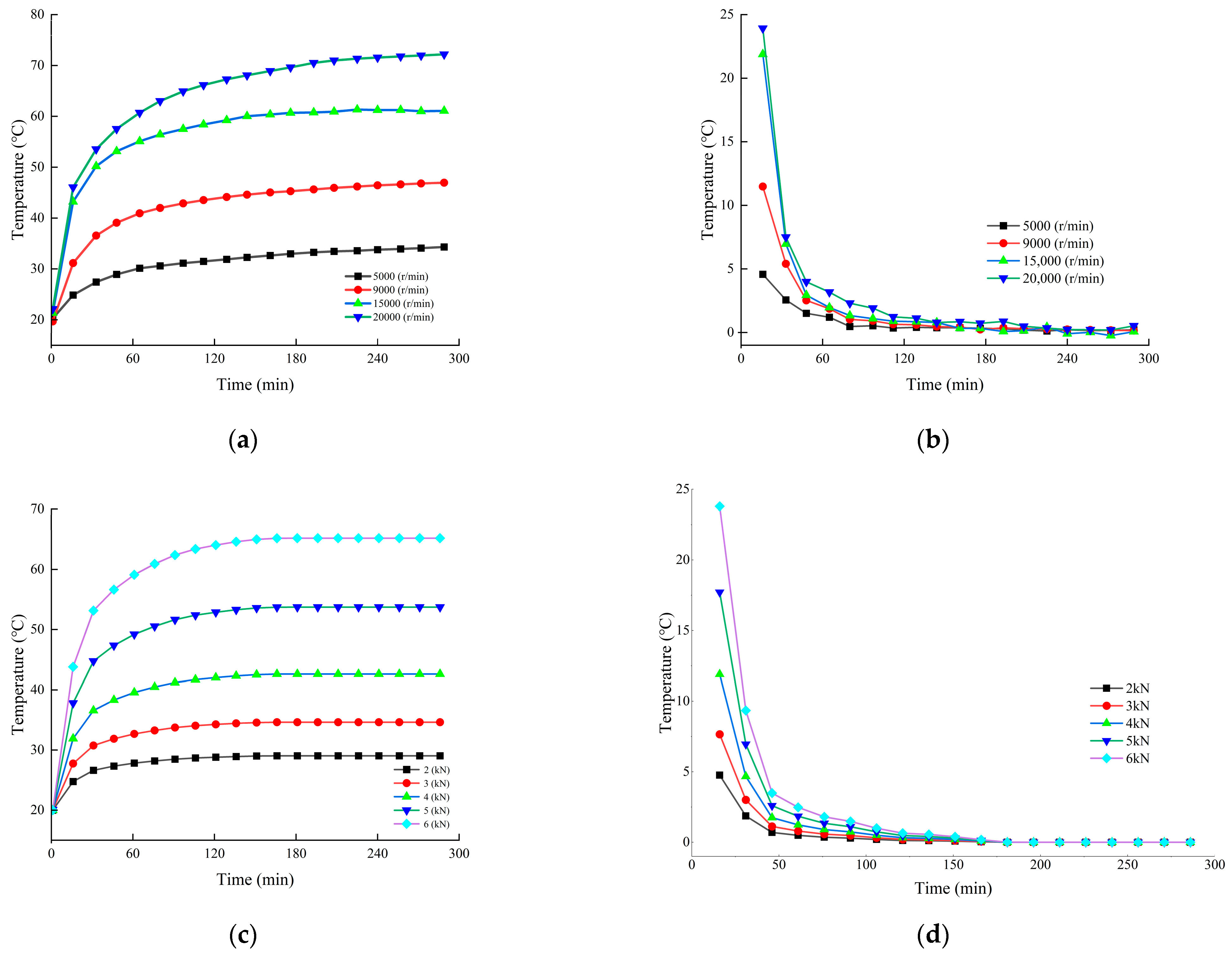
The temperature rise process and temperature rise rate of the bearing under constant operating conditions are shown in Figure 12. In Figure 12a, the conditions are radial load 2 kN , speeds 5000 r / min , 9000 r / min , 15,000 r / min , and 20,000 r / min . In Figure 12c, the conditions are test speed 3600 r / min , loads 1 kN , 2 kN , 3 kN , 4 kN , 5 kN and 6 kN . From Figure 12a,b, it can be concluded that under a fixed load, the final steady-state temperature of the bearing is proportional to the speed. The temperature rise rate of the bearing increases with higher speeds. As the speed increases, the bearing slip rate may become higher, and the frequency of rolling friction and sliding friction between the rolling elements and the raceway increases. The continuously changing contact points generate more frictional losses, resulting in more converted heat and a faster and higher temperature rise. From Figure 12c,d, it can be concluded that under a fixed speed, the final steady-state temperature of the bearing is also proportional to the load. The temperature rise rate of the bearing increases with higher loads. The temperature rise in the bearing is relatively intense within the first 60 min. As time progresses, the temperature rise becomes increasingly smaller, and the final temperature fluctuates within a certain range. Based on the temperature rise rate, the bearing temperature rise process can be divided into a temperature rise phase and a steady-state phase.
2.
Bearing Temperature Rise Characteristics under Variable-Speed Conditions
The parameter settings for the variable-speed conditions are shown in Table 1. The bearing temperature rise process under variable-speed conditions is illustrated in Figure 13. Under variable-speed conditions, the overall trend of bearing temperature rise remains consistent with that under constant operating conditions and can also be divided into a temperature rise phase and a steady-state phase. However, the time required to reach the steady-state phase is longer, and the temperature fluctuation range during the steady-state phase is larger, with a variation of up to 2 °C.

7. Conclusions

This paper proposes a data–model integration-driven method for predicting the temperature rise in new energy electric drive bearings. A hybrid dataset was constructed using simulation data generated by a data–model integrated simulation model and measured data. The proposed CNN-LSTM model was employed to predict the bearing temperature rise process. Through experimental validation, the following conclusions were drawn:
  • The prediction error of the proposed method remains within 1 °C compared to the measured data. Specifically, under constant operating conditions, the maximum error during the temperature rise phase is 0.773 °C, and the maximum error during the steady-state phase is 0.686 °C. Under variable operating conditions, the maximum error during the temperature rise phase is 0.713 °C, and the maximum error during the steady-state phase is 0.764 °C. The CNN-LSTM model demonstrates superior prediction accuracy compared to the BP and LSTM models.
  • The feasibility of the data–model integration-driven method for predicting the temperature rise in new energy electric drive bearings was validated, providing an important technical reference for similar studies under comparable working conditions.
  • The bearing temperature rise process can be divided into a temperature rise phase and a steady-state phase, regardless of constant or variable operating conditions. The temperature changes rapidly during the temperature rise phase, while it fluctuates within a certain range during the steady-state phase. Under variable operating conditions, the temperature exhibits more pronounced fluctuations during the steady-state phase.

Limitations and Prospects

In the study of varying operating conditions, current research has primarily focused on scenarios with continuous changes in rotational speed. Future work could further expand the scope to investigate the impact of load variations on the characteristics of electric drive bearings. Actual working conditions are far more complex than experimental conditions, and subsequent studies should validate and analyze the proposed methods using real-world operational data.

Author Contributions

Conceptualization, F.Y. and X.C.; methodology, F.Y. and X.C.; validation, F.Y., X.C. and Z.Z.; supervision, J.Y. and W.Z.; writing—original draft preparation, X.C.; writing—review and editing, F.Y. and X.C. All authors have read and agreed to the published version of the manuscript.

Funding

This research was funded by Major Science and Technology Project of Henan Province, grant number 251100220200.

Data Availability Statement

Data are contained within the article.

Conflicts of Interest

The authors declare no conflicts of interest.

Abbreviations

The following abbreviations are used in this manuscript:
MAEMean Absolute Error
DNNDeep Neural Networks
LSTMLong Short-Term Memory Network
FNNFeedforward Neural Networks
GRNNGeneralized Regression Neural Networks
BPBack Propagation Neural Network
PSOParticle Swarm Optimization
CNNConvolutional Neural Network
GAGenetic Algorithm
RULRemaining Useful Life

References

  1. Cheng, Y.; Wang, Z.; Zhang, W. A Novel Condition-Monitoring Method for Axle-Box Bearings of High-Speed Trains Using Temperature Sensor Signals. IEEE Sens. J. 2019, 19, 205–213. [Google Scholar] [CrossRef]
  2. Li, C.; Feng, Q.; Sun, B.; Gao, L.; Jia, M.; Fang, Z.; Xiong, J. Wireless Method for Measuring the Rotational Speed of Roller Bearing in a High-Temperature Environment. IEEE Sens. J. 2022, 22, 20989–20998. [Google Scholar] [CrossRef]
  3. Palmgren, A. Ball and Roller Bearing Engineering: Theory Design and Application, 3rd ed.; SKF Industries: Blue Bell, PA, USA, 1959; pp. 225–230. [Google Scholar]
  4. Goncalves, D.; Cousseau, T.; Gama, A.; Campos, A.V.; Seabra, J.H. Friction torque in thrust roller bearings lubricated with greases, their base oils and bleed-oils. Tribol. Int. 2017, 107, 306–319. [Google Scholar] [CrossRef]
  5. Gao, P.; Tang, W.; Cui, Y.; Wang, Y.; Mo, G.; Yin, J. Theoretical and Experimental Investigation on Thermal Characteristics of Railway Double-Row Tapered Roller Bearing. Energies 2022, 15, 4217. [Google Scholar] [CrossRef]
  6. Yun, X.; Xie, F.; Han, Q. Study on bearing mechanical and thermal characteristic evolvement rules affected by higher ambient temperature. J. Vibroeng. 2022, 24, 1249–1261. [Google Scholar] [CrossRef]
  7. Chen, J.; Zhang, W.; Wang, H. Intelligent bearing structure and temperature field analysis based on finite element simulation for sustainable and green manufacturing. J. Intell. Manuf. 2021, 32, 745–756. [Google Scholar] [CrossRef]
  8. Cui, L.; He, Y.F.; Fu, F.W. Friction and temperature analysis of angular contact ball bearing in high speed electric spindle system. In Proceedings of the International Conference on Mechanics and Mechatronics, Changsha, China, 13–15 March 2015. [Google Scholar] [CrossRef]
  9. Kim, K.S.; Lee, D.W.; Lee, S.M.; Lee, S.J.; Hwang, J.H. A numerical approach to determine the frictional torque and temperature of an angular contact ball bearing in a spindle system. Int. J. Precis. Eng. Manuf. 2015, 16, 135–142. [Google Scholar] [CrossRef]
  10. Ye, Z.H.; Wang, L.Q.; Chen, G.C.; Tang, D. Analysis of thermo-mechanical coupling of high-speed angular-contact ball bearings. Adv. Mech. Eng. 2017, 9, 6. [Google Scholar] [CrossRef]
  11. Zhao, W.; Zhang, C.; Wang, J.; Wang, S.; Lv, D.; Qin, F. Research on Digital Twin Driven Rolling Bearing Model-Data Fusion Life Prediction Method. IEEE Access 2023, 11, 48611–48627. [Google Scholar] [CrossRef]
  12. Qin, Y.; Wu, X.; Luo, J. Data-Model Combined Driven Digital Twin of Life-Cycle Rolling Bearing. IEEE Trans. Ind. Inf. 2022, 18, 1530–1540. [Google Scholar] [CrossRef]
  13. Shi, H.; Song, Z.; Bai, X.; Hu, Y.; Li, T.; Zhang, K. A novel digital twin model for dynamical updating and real-time mapping of local defect extension in rolling bearings. Mech. Syst. Signal Process. 2023, 193, 110255. [Google Scholar] [CrossRef]
  14. Yang, J.; Palazzolo, A. Tilt Pad Bearing Distributed Pad Inlet Temperature with Machine Learning—Part I: Static and Dynamic Characteristics. J. Tribol. 2022, 144, 061801. [Google Scholar] [CrossRef]
  15. Yang, J.; Palazzolo, A. Tilt pad bearing distributed pad inlet temperature with machine learning—Part II: Morton effect. J. Tribol. 2022, 144, 061802. [Google Scholar] [CrossRef]
  16. Zhu, Y.; Cheng, J.; Liu, Z.; Zou, X.; Wang, Z.; Cheng, Q.; Xu, H.; Wang, Y.; Tao, F. Remaining Useful Life Prediction Approach Based on Data Model Fusion: An Application in Rolling Bearings. IEEE Sens. J. 2024, 24, 42230–42244. [Google Scholar] [CrossRef]
  17. An, Y.; Zhang, K.; Liu, Q.; Chai, Y.; Huang, X. Rolling Bearing Fault Diagnosis Method Base on Periodic Sparse Attention and LSTM. IEEE Sens. J. 2022, 22, 12044–12053. [Google Scholar] [CrossRef]
  18. Badawi, M.B.; Awad Taher, H.; El Fahham, I.M. Application of artificial intelligence for the prediction of plain journal bearings performance. Alex. Eng. J. 2022, 61, 9011–9029. [Google Scholar] [CrossRef]
  19. Zhou, E.; Zhao, Y.; Dai, Y.; Zhang, J.; Zhang, Y.; Li, H. Research on Temperature Field Prediction Model of Electric Spindle Based on Improved BP Neural Network. Res. Sq. 2021. [Google Scholar] [CrossRef]
  20. Li, H.; Liu, C.; Yang, F.; Ma, X.; Guo, N.; Sui, X.; Wang, X. Dynamic Temperature Prediction on High-Speed Angular Contact Ball Bearings of Machine Tool Spindles Based on CNN and Informer. Lubricants 2023, 11, 343. [Google Scholar] [CrossRef]
  21. Deng, C.; An, L.; Cheng, X.; Qu, J.; Gao, Z.; An, Q. A friction temperature model for dynamic bearing operation based on neural network and genetic algorithm. Tribol. Int. 2024, 191, 109057. [Google Scholar] [CrossRef]
  22. Li, J.; Li, Z.; An, B.; Li, R. Prediction of scuffing failure in grease-lubricated ball bearing based on GA-BP neural network. Eng. Fail. Anal. 2025, 170, 109331. [Google Scholar] [CrossRef]
  23. Lu, W.; Wang, Y.; Zhang, M.; Gu, J. Physics guided neural network: Remaining useful life prediction of rolling bearings using long short-term memory network through dynamic weighting of degradation process. Eng. Appl. Artif. Intell. 2024, 127, 107350. [Google Scholar] [CrossRef]
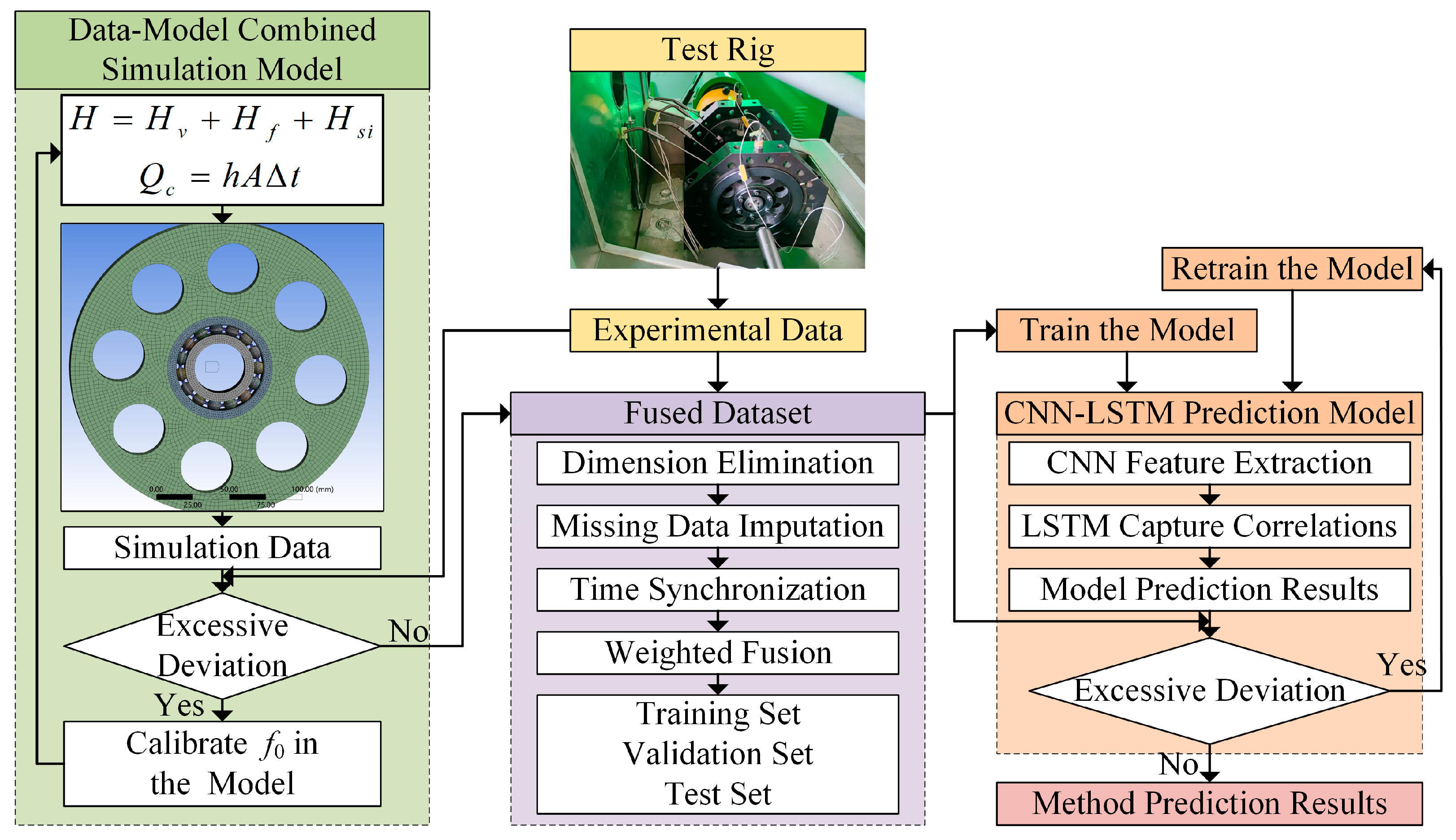
Figure 1. Framework of the temperature rise prediction method for new energy electric drive bearings.
Machines 13 00925 g001
Figure 2. Construction method of the temperature rise simulation model for new energy electric drive bearings based on data–model integration.
Machines 13 00925 g002
Figure 3. Finite element simulation model.
Machines 13 00925 g003
Figure 4. Structure and data flow of the CNN-LSTM temperature rise prediction model.
Machines 13 00925 g004
Figure 5. New energy electric drive bearing performance test rig and layout of temperature measurement points.
Machines 13 00925 g005
Figure 6. Simulation and experimental temperature results: (a) Simulated and measured temperature comparison at different speeds; (b) simulated temperature error at different speeds; (c) simulated and measured temperature comparison at different loads; (d) simulated temperature error at different loads; (e) simulated and measured temperature comparison at slowly varying speed conditions; (f) simulated temperature error at slowly varying speed conditions.
Machines 13 00925 g006
Figure 7. Displays a subset of the dataset: (a) Measured Data for Conditions 1–4; (b) Simulation data are also included: (b1) radial load: 2 kN ; (b2) speeds: 3600 r / min ; (b3) speeds: 4200–6600 r / min .
Machines 13 00925 g007
Figure 8. Prediction results and prediction errors of different models: (a) prediction results; (b) prediction error.
Machines 13 00925 g008
Figure 9. MAE prediction of each model under slow speed conditions: (a) thermal transient stage and load is 2 kN; (b) thermal equilibrium stage and load is 2 kN; (c) thermal transient stage and rotational speed is 3600 r / min ; (d) thermal equilibrium stage and rotational speed is 3600 r / min .
Machines 13 00925 g009
Figure 10. Prediction results and prediction errors of different models: (a) CNN-LSTM prediction results; (b) LSTM prediction results; (c) BP prediction results; (d) Prediction errors.
Machines 13 00925 g010
Figure 11. MAE prediction of each model under slow speed conditions (load 2 kN ): (a) thermal transient stage; (b) thermal equilibrium stage.
Machines 13 00925 g011
Figure 12. Temperature rise characteristics of new energy electric drive bearings under constant operating conditions: (a) effect of speed on bearing temperature rise; (b) effect of speed on temperature rise rate; (c) effect of load on bearing temperature rise; (d) effect of load on temperature rise rate.
Machines 13 00925 g012
Figure 13. Temperature rise characteristics of new energy electric drive bearings under variable operating conditions: (a) bearing temperature rise; (b) bearing temperature rise rate.
Machines 13 00925 g013
Table 1. Parameter setting of bearing speed change.
Test StepSpeed (r/min)Time (s)Radial Load (kN)Axial Load (kN)
10~540031.7990.257
2540061.7990.257
35400~18,00061.7990.257
418,000181.7990.257
518,000~540061.7990.257
Note: The test Begin with Step 1, then loop through Steps 2 to 5 for 40,000 cycles.
Table 2. Maximum simulation error and MAE under different working conditions.
No.Condition Maximum   Error   ( ° C ) MAE   ( ° C )
1condition 11.5991.074
2condition 21.5881.025
3condition 30.8160.516
4condition 41.3970.911
5gradual variable-speed condition1.5770.749
Table 3. Model parameters.
Parameter NameParameter Value
number of convolutional layers2
kernel size7 × 7/3 × 3
number of kernels64/128
LSTM hidden layers count1
LSTM units per LSTM layer128
Disclaimer/Publisher’s Note: The statements, opinions and data contained in all publications are solely those of the individual author(s) and contributor(s) and not of MDPI and/or the editor(s). MDPI and/or the editor(s) disclaim responsibility for any injury to people or property resulting from any ideas, methods, instructions or products referred to in the content.